An Adaptive Parameter-Free Optimal Number of Market Segments Estimation Algorithm Based on a New Internal Validity Index

1  Introduction

Market segmentation is an important marketing tool that aims to divide a large heterogeneous market into several small homogeneous markets so that consumers located in the same sub-market have similar demands and consumers located in different sub-markets have different demands, and enterprises can focus their resources on the most appropriate target market to maximize their interests [1]. So far, there have been many studies on the market segmentation bases and methods, but few studies on how to determine the optimal number of market segments (ONS) [2–4]; however, in practice, a reasonable ONS is a premise for carrying out a valuable market segmentation, because (1) different ONSs will directly change the composition of the market segmentation results, and the unrealistic sub-markets will mislead the enterprises to make relevant decisions, and (2) most current market segmentation methods need to be provided with the ONS in advance. Obviously, it is practical to strengthen the studies on how to determine an appropriate ONS.

In the state-of-the-art studies, there are two main ways to determine the ONS: (1) the researchers directly specify an ONS or a range based on their prior knowledge [5], and (2) the combination of a validity index and a clustering algorithm is used to determine the ONS due to a fact that the clustering analysis is the current dominant market segmentation technique and most clustering algorithms also require a pre-specified number of clusters (NC), which makes the process of finding the optimal NC (ONC) coincide with the purpose of determining the ONS [6]. Compared with the former, this combination strategy is more objective and user-friendly; and its basic idea is to perform a clustering algorithm many times with different NCs, choose an appropriate validity index to evaluate the clustering results, and determine the ONC (ONS) according to the evaluation values [7,8], in which the selections of the validity index and the clustering algorithm play the very important roles in whether a reasonable ONC can be obtained. And in our study, we also try to propose an effective method for determining the ONC based on such combinatorial idea.

For the validity indices, there are two main types: the external validity index (EVI) and internal validity index (IVI) [9]. Since the former is used with known data labels, while the latter is independent of the data labels, the IVIs can often be combined with the clustering algorithms to determine the ONC, where the Dunn index, Davies–Bouldin (DB) index, Silhouette (Sil) index and Calinski-Harabasz (CH) index are the most commonly used IVIs in the current literature [10]; and all of them evaluate the clustering results from two aspects, compactness and separation. Based on the Sil, Zhou et al. [11] proposed a new IVI CIP that can obtain more accurate ONC than the DB, Sil, Krzanowski-Lai (KL) index, Weighted inter-intra (Wint) index and In-group proportion (IGP) index with different clustering algorithms; particularly, they pointed out that although the CIP still mainly considers the compactness and separability, a valid IVI should consider compactness, separation and connectivity simultaneously and they provided the concept of the cluster connectivity qualitatively. In a recent study, Zhou et al. [7] also proposed a valid IVI BWC and it has been proved to be significantly better than the CH, DB, Sil, KL, Wint, Hartigan (Hart) index, IGP, Dunn and PBM index in terms of the ONC estimation, however, its definition still does not reflect the cluster connectivity. Unlike the compactness and the separation, the cluster connectivity refers to the fact that a sample should be classified into the same cluster with its neighboring samples, and they evaluate the reasonableness of the clustering results from three different perspectives. Thus, it is possible to quantitatively design a definition of the cluster connectivity and integrate it into the IVI to further improve the accuracy of the estimated ONC (EONC).

In terms of the clustering algorithms, the K-means algorithm (KMA) and its variants are commonly used clustering algorithms in combination with the IVIs for choosing the ONC since they are simple to implement and have linear time complexity [7]. For example, He et al. [12] combined the Sil with the KMA to estimate the ONC; Sheikhhosseini et al. [13] also chose the KMA as the basic algorithm from numerous clustering algorithms, and further combined it with the Davies–Bouldin’s measure and Chou–Su–Lai’s measure together to determine the ONC. Nevertheless, since the KMA is sensitive to the initial cluster centers (ICCs), and different ICCs tend to lead to different clustering results, as well as different clustering results will cause unstable ONCs, the traditional KMA is not the best choice for determining the ONC in combination with the IVIs [14]. In a recent study, Du et al. [15] successfully integrated the DB with a new clustering algorithm SDK-means++ to detect the ONC. Compared with the existing models, the SDK-means++ is stable and does not require setting any parameters, but it still suffers from two major shortcomings: (1) when calculating the first ICC, the setting of the parameter cut-off distance lacks theoretical support; and (2) when determining the remaining ICCs, the noises and edge points are more easily identified as ICCs, thus affecting the number of iterations (NI) of the algorithm and the final clustering performance. Therefore, it is necessary to further optimize the SDK-means++ to make it more suitable for determining the ONC in combination with the IVIs.

In our study, we proposed an adaptive parameter-free BWCON-NSDK-means++ algorithm for determining the ONC by integrating a new IVI and a new stable clustering algorithm. First, since the existing IVIs ignore the cluster connectivity, to complete the evaluation dimensions of the existing IVIs and evaluate a clustering result more comprehensively, we designed a cluster connectivity formula for the first time based on the neighbor relationship, and thus defined a new IVI, Between-Within-Connectivity (BWCON), to evaluate the clustering results from three dimensions of compactness, separation and connectivity. Then, to address the aforementioned problems in the SDK-means++, we chose the sample with the most natural neighbors as the first ICC to solve the parameter problem, and introduced a modification mechanism in the original SDK-means++ to address the noise and the edge point problems, and finally proposed the Natural-SDK-means++ (NSDK-means++) algorithm for combination with the IVI. At last, considering that the existing combination strategies usually take the NC corresponding to the maximum or minimum evaluation value as the ONC, ignoring the fact that such values are easily disturbed by the special points or clusters in the clustering results, we developed a novel ONC estimation framework based on the proposed BWCON, and proposed an independent and objective ONC estimation algorithm BWCON-NSDK-means++ by effectively integrating the NSDK-means++ into this framework. The experimental results obtained show that the BWCON index is able to better estimate the ONC than those previous IVIs such as Dunn, DB, Sil, CH, BWP, CIP and BWC with different clustering algorithms on the seven UCI datasets and five synthetic datasets; on these relatively complex UCI datasets, the proposed NSDK-means++ can achieve the better clustering performance than other five existing clustering algorithms in terms of nine validity indices; moreover, the BWCON-NSDK-means++ is proved to be able to obtain more accurate ONC than the BWCON-KMA, BWCON-MBK, BWCON-KM++, BWCON-RKM++, BWCON-SDKM++, BWCON-Single linkage, BWCON-Complete linkage, BWCON-Average linkage and BWCON-Ward linkage algorithms on all twelve datasets, and can be used as a stand-alone market segmentation tool.

The rest of this paper is organized as follows. The overview of different IVIs and clustering algorithms is presented in Section 2. Section 3 introduces the proposed BWCON-NSDK-means++ algorithm in detail. Experimental results are provided in Sections 4 and 5. Finally, Section 6 summarizes the paper.

2  Related Work

In the following subsections, different IVIs and clustering algorithms are delineated.

2.1 Internal Validity Indices

Many IVIs have been proposed to evaluate the clustering performance and combined with the clustering algorithms to determine the ONC. Dunn [16] proposed the Dunn by combining the within-cluster and between-cluster distances, in which the within-cluster distance is estimated by calculating the maximum distance in any cluster, and the between-cluster distance is measured by calculating the shortest distance between samples in any two clusters; the larger the Dunn, the better the clustering results. In 1979, Davies et al. [17] proposed the DB, which is obtained from the ratio of within-cluster compactness and between-cluster separation; the minimization of the index shows better clustering partitions. In [18], Rousseeuw proposed the well-known Sil. Similar to the previous two indices, the Sil also evaluates the clustering results from two dimensions of compactness and separation; it measures the compactness of a sample by calculating the average distance from this sample to the other samples in this cluster and the separation of a sample by calculating the minimum value of average distance between this sample and samples in every other cluster. The Sil obtains its maximum value when the ONC is achieved. In 1974, Calinski et al. [19] proposed the CH that introduced the within-groups sum of squared and the between-groups sum of squared error to measure the compactness and separation; and similarly, the ONC corresponds to the maximum CH. In 2011, Zhou et al. [20] proposed the BWP index, in which the compactness and separation measures are exactly the same as those of the Sil, and the only difference between them is that their normalization methods are different: the BWP used the clustering distance to normalize itself; theoretical studies and experimental results have shown that the BWP significantly outperforms the DB, KL, Homogeneity-Separation (HS) and IGP in terms of the ONC estimation. To improve the time performance of the Sil and BWP, Zhou et al. [11] proposed a new IVI, CIP, based on the concept of the sample geometry, which measures the compactness of a sample by calculating the distance from this sample to the centroid of this cluster, and the separation of a sample by calculating the minimum distance between this sample and every centroid of other clusters; the obtained results show that the CIP can obtain the accurate NC more quickly than the existing indices. In a recent study, Zhou et al. [7] further improved the Sil and proposed the BWC that still evaluates the clustering results from two aspects of compactness and separation, where it measures the compactness of a cluster by calculating the average distance between every sample of this cluster and its centroid, and the separation of a cluster by calculating the minimum distance between the centroid and every centroid of other clusters; and the ONC is obtained at the maximum BWC under different NCs.

It can be seen that in terms of the ONC estimation, although the validity of all of the above indices has been proved on various datasets with different clustering algorithms, none of them consider the cluster connectivity. The cluster connectivity measures the reasonableness of the clustering results from a neighborhood perspective, and it is of great practical significance to give a quantitative formula for calculating the connectivity and incorporate it into the IVIs to evaluate the clustering results together with the compactness and the separation. In addition, when searching for the ONC, the existing IVIs often determine the ONC by finding their maximum or minimum values under different NCs, however, such values are easily dominated by the locations of the special points or clusters in the clustering results, which will in turn directly affect the final estimates.

2.2 Clustering Algorithms

In the literature, there are two main types of clustering algorithms that are often combined with IVIs to determine the ONC: hierarchical and partitional clustering [8]. For the hierarchical clustering, according to the direction of clustering, there are two types of methods: agglomerative hierarchical clustering (AHC) and divisive hierarchical clustering (DHC) [21], where the former follows the bottom-top strategy, which treats each sample as a complete cluster at the beginning, and then gradually merges them into some larger cluster based on a certain criterion, and on the contrary, the DHC adopts the top-down strategy, which initially regards the entire dataset as a complete cluster and then splits the dataset into some smaller clusters based on a certain criterion [22]. Compared with the DHC, the AHC is more accurate and widely used [23], and in recent years, the classic AHC with single linkage, complete linkage, average linkage and ward linkage are still the most widely used AHC methods [24,25]. In general, the AHC is simple in idea and has the stable clustering performance, but it is not suitable for clustering large datasets due to its high time complexity [24].

While among the partitional clustering algorithms, the KMA is currently the most popular one, and its implementation consists of five main steps: (1) specify the NC m; (2) select m samples randomly as the ICCs; (3) classify each sample into the cluster where its nearest center is located; (4) update the clustering centers by treating the mean of each cluster as a new center; and (5) repeat Steps (3) and (4) until the clustering centers no longer change [26]. In a subsequent study, Sculley [27] improved the KMA and proposed the Mini-batch K-means (MBK) to accelerate the clustering speed by randomly selecting a subset instead of the whole dataset to train the ICCs, but like KMA, its clustering performance is unstable and very sensitive to the ICCs [28]. A representative partition-based clustering algorithm K-means++ proposed by Arthur and Vassilvitskii provided such an effective solution to determine the ICCs, as shown in Algorithm 1, in which the ICCs are determined based on a D2 weighting method following the principle that the larger the distances among the ICCs, the more reasonable the selection of the ICCs, and it can effectively reduce the possibility of multiple ICCs appearing in the same cluster [29]. However, due to the existence of the line 1 in the Algorithm 1, the K-means++ still has a certain degree of randomness.

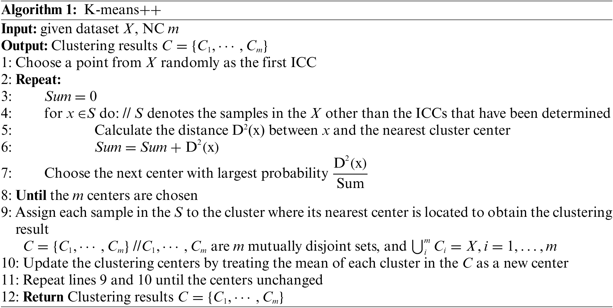
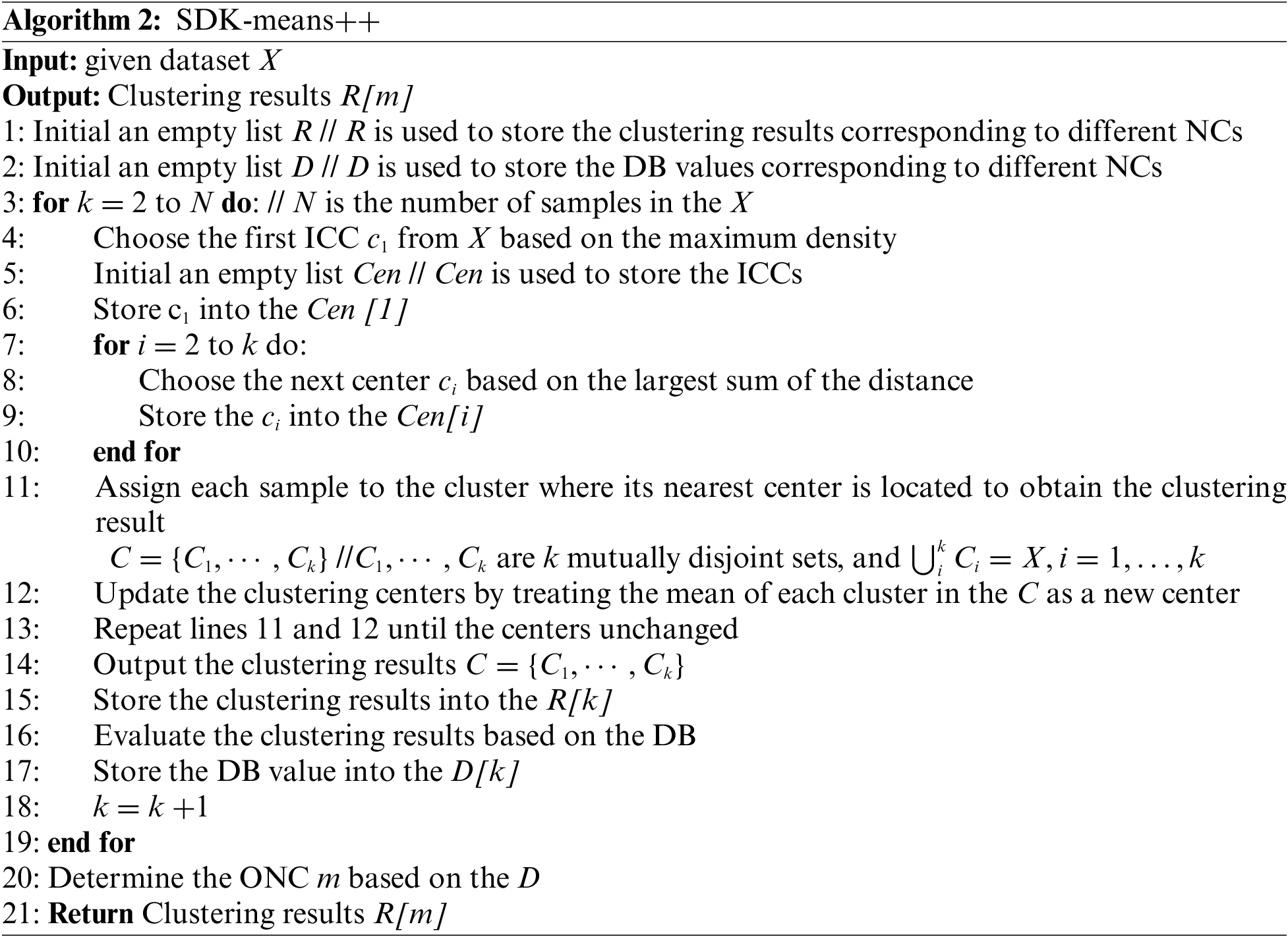
In [30], an alternative way to determine the ICCs is introduced in the K-means++, called RK-means++ in our study that determines the ICCs by randomly selecting a random value, and then weighting to calculate the ICCs; it is still unstable since (1) the first ICC is generated randomly, and (2) the determination of the remaining ICCs requires first choosing a small random number at random. To completely solve the randomness problem, the SDK-means++ was proposed in 2021 based on the DB, maximum density and the largest sum of distance, as shown in Algorithm 2, in which the IVI DB is used to adaptively determine the ONC to avoid artificially setting the parameter NC, the maximum density is utilized to determine the first ICC to avoid the randomness, and the largest sum of distance is designed to ensure that all ICCs are generated in different clusters, but as mentioned in the introduction, its parameter, noise and edge point issues can be further optimized [15].

3  Proposed Work

In all the following works, the Euclidean distance is used to evaluate the dissimilarity.

3.1 The IVI: The BWCON Index

Definition 1 Let dataset X={x1,x2,…,xN}, and xi is the ith sample. Assuming that N samples are clustered into m clusters, the centroid μk of the cluster k is defined as the mean value of all samples in the cluster k, i.e.,

μk=1nk∑p=1nkxp(k)(1)

where k represents the cluster label, xp(k) represents the pth sample in the cluster k, and nk represents the number of samples in the cluster k.

Definition 2 Let dataset X={x1,x2,…,xN}, and xi is the ith sample. Assuming that N samples are clustered into m clusters, the within-cluster distance wc(j) of cluster j is defined as the average distance between every point in the cluster j and the centroid of cluster j, i.e.,

wc(j)=1nj∑i=1nj‖Xi(j)−μj‖(2)

where j represents the cluster label, xi(j) represents the ith sample in the cluster j, ‖.‖ represents the Euclidean distance, and nj represents the number of samples in the cluster j.

Definition 3 Let dataset X={x1,x2,…,xN}, and xi is the ith sample. Assuming that N samples are clustered into m clusters, the between-cluster distance bc(j) of cluster j is defined as the average distance between the centroid of cluster j and every centroid of other clusters, i.e.,

bc(j)=1m−1∑1≤k≤m,k≠j‖μj−μk‖(3)

where j and k represent the cluster label.

Definition 4 Let dataset X={x1,x2,…,xN}, and xi is the ith sample. Assuming that N samples are clustered into m clusters, the connectivity con(j,i) of xi(j) is defined as the ratio of the length of the intersection of the KNNT(xi(j)) and KNNT(xi(j))′ to T, i.e.,

con(j,i)=length(KNNT(xi(j))∩KNNT(xi(j))')T(4)

where the connectivity con(j,i) of sample xi(j) is the ratio of the number of samples that are classified into the j among all T nearest neighbors of xi(j) to T. Specifically, T is the number of neighboring samples determined using the Algorithm 1 in [31] that is an adaptive method for determining the number of nearest neighbors for a dataset to be clustered, KNNT(xi(j)) represents the T nearest samples to xi(j) in the whole dataset and KNNT(xi(j))' denotes the T nearest samples to xi(j) in the cluster j. Moreover, when nj≤T, KNNT(xi(j))' are all samples in the cluster j.

Definition 5 Let dataset X={x1,x2,…,xN}, and xi is the ith sample. Assuming that N samples are clustered into m clusters, the connectivity con(j) of cluster j is defined as the mean of the connectivity values of all samples in the cluster j, i.e.,

con(j)=1nj∑i=1njcon(j,i)(5)

where nj represents the number of samples in the cluster j.

Definition 6 Let dataset X={x1,x2,…,xN}, and xi is the ith sample. Assuming that N samples are clustered into m clusters, the BWCON of cluster j BWCON(j) is as follows:

BWCON(j)=[wc(j),bc(j),con(j)](6)

In Definition (6), the BWCON consists of three evaluation dimensions. For the compactness, we use wc(j) defined in (2) to reflect the overall compactness of cluster j, and the smaller value of wc(j) represents the high cluster compactness. For the separation, the bc(j) defined in (3) is used to reflect the between-cluster separation of cluster j; and the large value of bc(j) shows the high cluster separation. Compared with the separation in the BWC, we replace the minimum distance between the centroid of cluster j and the centroids of other clusters in the clustering results with the average distance, which can better reflect the structural relationship between this cluster and other clusters on the whole. As for the cluster connectivity, we use con(j,i) defined in (4) to reflect the connectivity of sample xi(j), and use con(j) defined in (5) to reflect the connectivity of cluster j. Extremely, if the T nearest neighbors of a sample in its cluster are exactly the same as its T nearest neighbors in the entire dataset, we consider that this sample is correctly classified in the dimension of connectivity; obviously, the larger the con(j) is, the more reasonable the clustering results are.

To understand the BWCON intuitively, we illustrate the BWCON by providing a distribution diagram of Fig. 1.

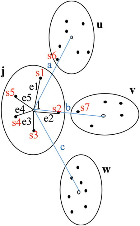
Figure 1: Distribution diagram of clustering structure for the BWCON index

In Fig. 1, the dataset consists of four clusters: j, u, v and w, the centroid of j is marked by l, the centroids of the other three clusters are represented by the hollow circles, and since the dataset is small, the T is directly specified as 1. According to Definitions 2 and 3, we can obtain that wc(j)=e1+e2+e3+e4+e55 and bc(j)=a+b+c3; according to Definitions 4 and 5, we can get that con(j,s1)=| KNN1(s1)∩KNN1(s1)' |1=| {s6}∩{s5} |=0, con(j,s2)=|KNN1(s2)∩KNN1(s2)' |1=| {s7}∩{s3} |=0, con(j,s3)=| KNN1(s3)∩KNN1(s3)' |1=| {s4}∩{s4} |=1, con(j,s4)=| KNN1(s4)∩KNN1(s4)' |1=| {s5}∩{s5} |=1, con(j,s5)=| KNN1(s5)∩KNN1(s5)' |1=| {s4}∩{s4} |=1, and con(j)=0+0+1+1+15=0.6; and ultimately, according to Eq. (6), the BWCON of j is [e1+e2+e3+e4+e55, a+b+c3, 0.6].

Furthermore, to evaluate the clustering validity of a whole dataset, the avgBWCON(m) function is defined.

Definition 7 Let dataset X={x1,x2,…,xN}, and xi is the ith sample. Assuming that N samples are clustered into m clusters, the avgBWCON(m) is defined as the average BWCON values of all clusters in the clustering results, i.e.,

avgBWCON(m)=[1m∑j=1mwc(j),1m∑j=1mbc(j),1m∑j=1mcon(j)](7)

3.2 The BWCON-Based ONC Estimation Framework

The main steps for estimating the ONC based on the BWCON are presented as follows:

Step 1: Cluster the input dataset under different NCs.

Let N be the number of samples, k is the NC, and the range of k is [2,⌊N⌋] as in [7,8,11]. The object of this step is to get different clustering results corresponding to different NCs under a certain clustering algorithm.

Step 2: Evaluate the above clustering results according to the BWCON.

In this Step, a BWCON matrix is generated, written as

(avgBWCON(2)avgBWCON(3)⋮avgBWCON(⌊N⌋))=([12∑j=12wc(j),12∑j=12bc(j),12∑j=12con(j)][13∑j=13wc(j),13∑j=13bc(j),13∑j=13con(j)]⋮[1⌊N⌋∑j=1⌊N⌋wc(j),1⌊N⌋∑j=1⌊N⌋bc(j),1⌊N⌋∑j=1⌊N⌋con(j)])(8)

Further, Eq. (8) is simplified as follows:

(avgBWCON(2)avgBWCON(3)⋮avgBWCON(⌊N⌋))=(wc2,bc2,con2wc3,bc3,con3⋮wc⌊N⌋,bc⌊N⌋,con⌊N⌋)(⌊N⌋−1)×3(9)

Step 3: Standardize the BWCON matrix.

Since the change trends of the compactness, separation and connectivity are different, they are standardized differently so that the larger the values of the standardized compactness, separation and connectivity, the better the clustering performance. Related calculations are shown in the Eqs. (10)–(12), and (13) is the standardized BWCON matrix.

Stdwcl=maxiwci−wclmaxiwci−miniwci,l=2,3,…,⌊N⌋,i=2,3,…,⌊N⌋(10)

Stdbcl=bcl−minibcimaxibci−minibci,l=2,3,…,⌊N⌋,i=2,3,…,⌊N⌋(11)

Stdconl=conl−miniconimaxiconi−miniconi,l=2,3,…,⌊N⌋,i=2,3,…,⌊N⌋(12)

Std(avgBWCON(2)avgBWCON(3)⋮avgBWCON(⌊N⌋))=(Stdwc2,Stdbc2,Stdcon2Stdwc3,Stdbc3,Stdcon3⋮Stdwc⌊N⌋,Stdbc⌊N⌋,Stdcon⌊N⌋)(⌊N⌋−1)×3(13)

Step 4: Estimate the ONCs under different dimensions in turn.

In this step, the compactness, separation and connectivity matrices, diffcom, diffsep and diffcon, are generated as follows:

diffcom=(Stdwc3−Stdwc2Stdwc4−Stdwc3⋮Stdwc⌊N⌋−Stdwc⌊N⌋−1)(⌊N⌋−2)×1(14)

diffsep=(Stdbc3−Stdbc2Stdbc4−Stdbc3⋮Stdbc⌊N⌋−Stdbc⌊N⌋−1)(⌊N⌋−2)×1(15)

diffcon=(Stdcon3−Stdcon2Stdcon4−Stdcon3⋮Stdcon⌊N⌋−Stdcon⌊N⌋−1)(⌊N⌋−2)×1(16)

Further, the ONCs, ncom, nsep and ncon, corresponding to the compactness, separability and connectivity, are calculated separately according to Eqs. (17)–(19).

ncom={v+1,|Stdwcv+1−Stdwcv|=max(|diffcom|),Stdwcv+1−Stdwcv>0v,|Stdwcv+1−Stdwcv|=max(|diffcom|),Stdwcv+1−Stdwcv≤0(17)

nsep={v+1,|Stdbcv+1−Stdbcv|=max(|diffsep|),Stdbcv+1−Stdbcv>0v,|Stdbcv+1−Stdbcv|=max(|diffsep|),Stdbcv+1−Stdbcv≤0(18)

ncon={v+1,|Stdconv+1−Stdconv|=max(|diffcon|),Stdconv+1−Stdconv>0v,|Stdconv+1−Stdconv|=max(|diffcon|),Stdconv+1−Stdconv≤0(19)

where 2≤v<⌊N⌋, and |⋅| means taking the absolute value.

Step 5: Determine the ONC.

The ONC, noptimal, is defined as

noptimal=round(ncom+nsep+ncon3)(20)

In Step 5, considering that the NC should be an integer, we perform a round operation; and compared with rounding up or rounding down, round can better fetch the NC that occurs more frequently in the [ncom,nsep,ncon]. For example, when [ncom,nsep,ncon] = [3, 2, 3], we obtain that round(3+2+3/3)=3, ⌊3+2+3/3⌋=2, ⌈3+2+3/3⌉=3, and 3 with the highest number of occurrences is obtained using the round and the rounding up; and when [ncom,nsep,ncon] = [2, 2, 3], we can obtain that round(2+2+3/3)=2, ⌊2+2+3/3⌋=2,⌈2+2+3/3⌉=3, and 2 is obtained using the round and the rounding down.

Here, to facilitate understanding, we use the commonly used Seeds from the UCI repository as an example and choose the stable AHC with the average linkage as our clustering algorithm to illustrate the above steps in more detail.

Step 1: Cluster the Seeds under different k, where, N is 210, the range of k is [2,14].

Step 2: According to Eq. (8), the BWCON matrix is shown below:

(avgBWCON(2)avgBWCON(3)⋮avgBWCON(14))=([1.94,6.07,0.98][1.51,5.41,0.96]⋮[0.73,5.27,0.65])

Step 3: According to Eqs. (10)–(12), the standardized BWCON matrix is as follows:

Std(avgBWCON(2)avgBWCON(3)⋮avgBWCON(14))=(0,1,10.35,0.39,0.93⋮1,0.26,0)

Step 4: The ncom, nsep and ncon are estimated according to Eqs. (14)–(19).

To facilitate the analysis, we visualize the diffcom, diffsep and diffcon in Fig. 2.

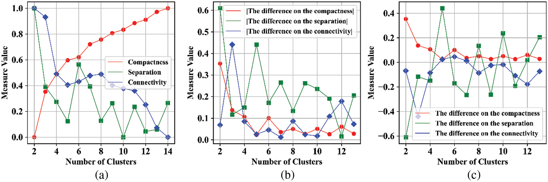
Figure 2: Schematic diagrams for the final ONC estimation

Fig. 2a shows the change trend of the compactness, separation and connectivity under different NCs, Fig. 2b presents the values of |diffcom|, |diffsep| and |diffcon|, and Fig. 2c represents the values of diffcom, diffsep and diffcon. In Fig. 2a, as the NC increases, the overall trend is upward for the red line and downward for the blue line, this is because the compactness and the connectivity of a cluster are only related to the distribution of the cluster itself, and with the increase of the NC, the sample size of each cluster in the clustering result becomes smaller and smaller, which means that the average distance from each point in the cluster to its centroid tends to become smaller and each sample is less and less likely to be grouped into the same cluster with its T nearest neighbors; obviously, it is unreliable to simply take the NCs corresponding to the maximum compactness or the maximum connectivity as the final determined ONCs. As for the separation, there is no such general rule because the separation of a cluster is related not only to the distribution of the cluster itself, but also to the distributions of other clusters in the clustering result. Thus, in our work, we only focus on the points with the largest fluctuations under different NCs as in Eqs. (17)–(19) to determine the corresponding ONCs since small fluctuations of these three measures are likely to be caused by some special points or clusters in the clustering results, and it is also unreliable to judge the reasonableness of the clustering result on this basis. Specifically, for the compactness, the point with the largest fluctuation is searched in Fig. 2a, and we can find that the fluctuation is maximum when the NC changes from 2 to 3 (as the first point on the red line in Fig. 2b), as well as the fluctuation is positive (as the first point on the red line in Fig. 2c), i.e., the clustering result has a higher compactness as the NC increases by 1; thus, according to Eq. (17), ncom = 3. Similarly, nsep=2 and ncon=3.

Step 5: According to Eq. (20), noptimal=3, which is consistent with the true NC (TNC).

3.3 The Adaptive Parameter-Free ONC Estimation Algorithm: BWCON-NSDK-Means++

From the illustration in Section 3.2, an IVI and a clustering algorithm are indispensable for determining the ONC. Here, we optimize the SDK-means++ algorithm and propose the NSDK-means++ to integrate with the above BWCON-based ONC estimation framework. And the process of the NSDK-means++ is described as follows:

Step 1: Input a dataset X={x1,x2,…,xN}, and the NC is m.

Step 2: Choose the first ICC c1 from X based on the fact: the ICCs should be distributed in the center of each cluster and surrounded by many samples.

Definition 8 Natural neighbor of a sample xi is defined as follows:

xj∈NN(xi)⇔xi∈KNNλ(xj)∧xj∈KNNλ(xi)(21)

In this step, the c1 is determined based on the concept of natural neighbor that is derived from [31]; where NN(xi) denotes a set of natural neighbors of point xi, the point xj is a natural neighbor of xi, λ is the number of neighboring samples, KNNλ(xj) is a set of λ nearest neighbors of xj, and KNNλ(xi) is a set of λ nearest neighbors of xi. It can be seen that when and only when xi belongs to one of λ nearest samples from xj and xj also belongs to one of λ nearest samples from xi, xj is called a natural neighbor of xi, that is to say, when xj is a natural neighbor of xi, these two samples are close to each other. Obviously, the more natural neighbors a point has, the more points it is surrounded by, and the more likely it is to be an ICC, thus in our study, we consider the point with the most natural neighbors as the c1. Meanwhile, to avoid parameter setting, we also determine the λ using the Algorithm 1 in [31] that is an adaptive method for determining the number of nearest neighbors for a dataset to be clustered.

Step 3: Choose the next center ci based on the largest sum of the distance.

To ensure that the distances among the ICCs are as large as possible and the obtained ICCs can be located in different clusters, we adopt the largest sum of the distance as in [15] to determine the next center ci, i.e.,

ci={sh|max{w(s1),⋯,w(sn)}}(22)

w(sj)=∑t=1hd(sj,ct),sj∈S,ct∈C(23)

where C denotes a set of ICCs that have been identified, S is a set of samples in the X other than the samples in the C, ct is an ICC in the C, sj is a sample in the S, d(⋅,⋅) represents the Euclidean distance, h is the number of samples in the C, n is the number of samples in the S, and the sample with the largest w(sj), j∈[1,n], is identified as the next ICC. It can be seen that the ICC selection method based on the largest sum of the distance links each new ICC with all existing ICCs, which ensures not only that there are the large differences among the ICCs, but also that the different ICCs are located in different clusters.

Step 4: Repeat Step 3 until the m centers c={c1,c2,⋯,cm} are chosen.

Step 5: Modify m centers in the c based on their respective λ neighboring samples.

In this step, to ensure that the final ICCs are located in the center of each cluster as much as possible and reduce the number of iterations of the ICCs, the obtained m centers are further modified, i.e.,

KNNλ(ci)=⋃r=1λ{findKNN(ci,r)}ci∈c(24)

ci'=Sum(KNNλ(ci))λ(25)

where ci is an ICC in the c, λ is the number of neighboring samples that is equal to λ in the Step 2 to avoid parameter setting, findKNN(ci,r) returns the rth nearest neighbor of ci, KNNλ(ci) is a set of λ nearest neighbors of ci, the mean value ci' of the λ nearest neighbors of the ci is the finalized ICC corresponding to the ci, and in our work, the modified m ICCs are denoted as c'={c1',c2',⋯,cm'}. The rationality of using the neighboring samples to modify the c is that a sample should be grouped in the same cluster as its neighboring samples, and by interacting with the neighboring samples as in Eq. (25), an ICC located at the edge can be moved closer to the inner part of the corresponding cluster.

Step 6: For each sample xi, calculate the distance to the m centers in the c' and assign it to the cluster with the smallest Euclidean distance; and the obtained clustering results are denoted as C={C1,⋯,Cm}, where ⋃imCi=X,i=1,…,m, and Ci∩Cj=ϕ, ∀i,j,i≠j,j=1,…,m.

Step 7: Update the c' by using the mean value of each cluster as the new center of the corresponding cluster.

Step 8: Repeat Steps 6 and 7 until the centers are unchanged.

Step 9: Output the clustering results C={C1,⋯,Cm}.

To visually illustrate the superiority of the NSDK-means++, Fig. 3 compares the ICCs obtained by the SDK-means++ with those obtained by the NSDK-means++.

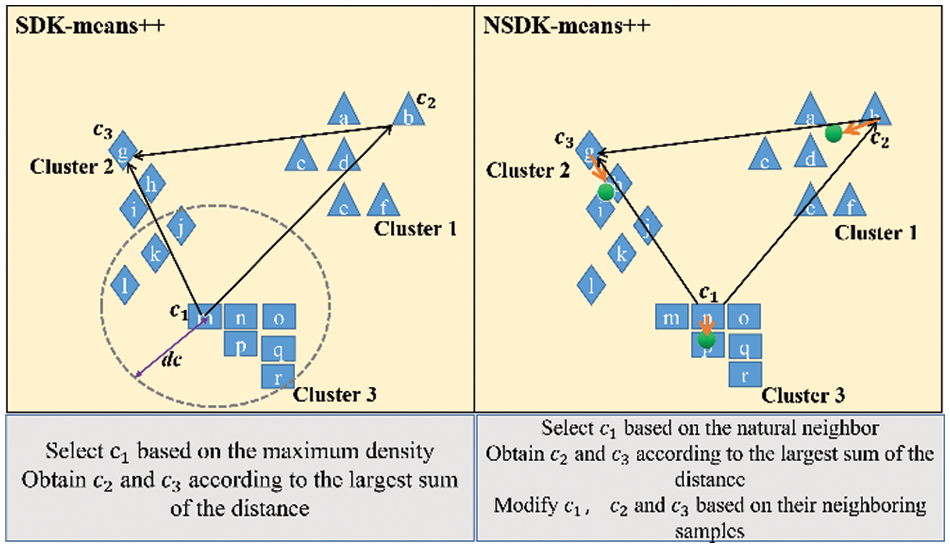
Figure 3: Schematic diagrams of the processes of determining the ICCs

In Fig. 3, the SDK-means++ estimates the density of each sample by counting the number of samples falling within the cut-off distance dc around each sample, with more samples indicating a higher density at that point, and in turn using the point with the highest density as the first ICC. In the figure on the left, we set the dc to be the radius of the gray circle, thus the point m is determined as the first ICC, and based on the Eqs. (22) and (23), the remaining two ICCs are, in order, b and g that are located at the edges of the clusters because the largest sum of the distance always determines the next ICC based on the furthest distance from the identified ICCs. For the NSDK-means++, because the dataset is small, we directly take λ as 1; for the point a in the Cluster 1,  KNN1(a)={d} and  KNN1(d)={a}, thus the number of natural neighbors of a is 1; similarly, the numbers of the natural neighbors of b to r are: 0, 0, 1, 1, 1, 0, 1, 1, 1, 1, 0, 1, 3, 1, 1, 1 and 1, thus point n is the first ICC determined, and the remaining ICCs are further determined as b and g based on the largest sum of the distance; moreover, the initial positions of these three ICCs are modified using their respective one neighboring sample (i.e., p, a and h) according to Eqs. (24) and (25), and ultimately, their positions moved from the edges of the clusters to the green dots along the orange arrows, which are closer to the inner parts of the clusters, and still distributed in the different clusters. Note that the orange arrows in the above diagram only qualitatively indicate the movement trend of the ICCs; and for the example above, the advantage of the Step 5 would be even more apparent if λ were to be increased slightly.

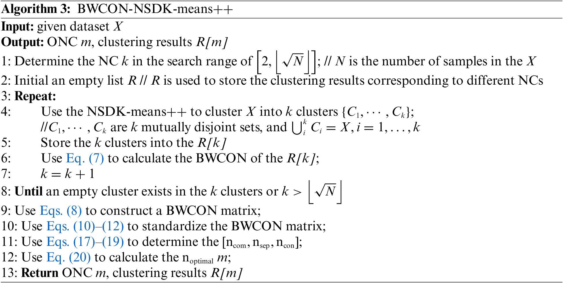
As a result, the BWCON-NSDK-means++ that can independently determine the ONC is proposed in Algorithm 3.

4  Experimental Studies

In this section, to demonstrate the effectiveness of the combination “BWCON+NSDK-means++”, we conduct three experiments: (1) to show that the BWCON is a more suitable IVI for determining the ONC than those already existing IVIs, we combine the BWCON and seven other IVIs with different clustering algorithms and compare their abilities to estimate the ONC; (2) to illustrate that the NSDK-means++ is a more appropriate algorithm than the KMA and its variants for determining the ONC in combination with IVIs, the clustering performance of the NSDK-means++ and other five partition-based clustering algorithms is compared on seven UCI datasets; and finally (3) to prove the superiority of the BWCON-NSDK-means++, we integrate several representative clustering algorithms into our proposed BWCON-based ONC estimation framework and compare their ONC accuracies. All works of this research are implemented using python 3.8, running on an 11th Gen Intel(R) Core (TM) i7-1165G7@2.80 GHz CPU with 16.0 GB RAM and windows 10-64-bit operating system; and the SPSS is used for the Kruskal–Wallis test and Friedman test.

4.1 Data Acquisition

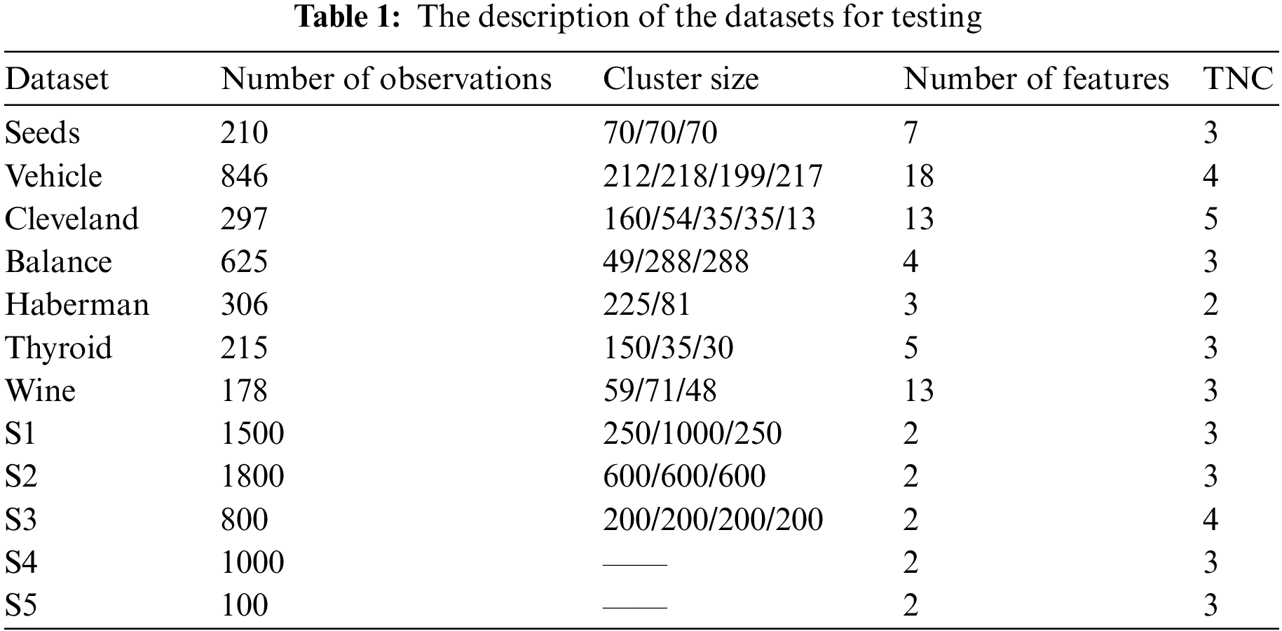
For validation purpose, the TNCs are known for all datasets used in this section, and the details of the selected datasets are shown in Table 1. Among them, Seeds, Vehicle, Cleveland, Balance, Haberman, Thyroid and Wine are the most commonly used public real-world datasets from the UCI Machine Learning Repository (http://archive.ics.uci.edu/ml/); S1, S2 and S3 are three 2-D synthetic datasets generated by using the “multivariate_normal” function from the numpy, and each cluster in these datasets is Gaussian-distributed; and S4 and S5 are generated using the “make_blobs” function of the sklearn. From Table 1, it can be seen that these datasets have different sample sizes (100–1800), features (2–18), NCs (2–5), and cluster sizes.

4.2 Superiority Evaluation of the BWCON-Based ONC Estimation Framework

To show the performance of the BWCON-based ONC estimation framework, like the existing studies [7,11], we choose the AHC with single linkage algorithm in combination with different IVIs to determine the ONC. In addition, the other four stable clustering algorithms are also adopted. In our study, all the above combinations are run within a search range [2,⌊N⌋]. The experimental results are shown in Tables 2–6, where the bold numbers indicate the correct NCs.

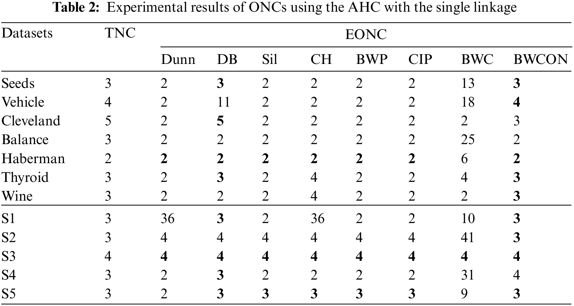
From Table 2, we can find that the Dunn is valid for the Haberman and S3, the DB is valid for all the datasets except Vehicle, Balance, Wine and S2, the Sil, CH, BWP and CIP are valid for the Haberman, S3 and S5, the BWC is valid for the S3, and our proposed BWCON is invalid only for Cleveland, Balance and S4. Meanwhile, it can be also seen that all the above indices are unable to get the correct NC for the Balance, and only BWCON can detect the correct NC for Vehicle, Wine and S2 datasets. Obviously, the combination “BWCON+AHC with the single linkage” has the best NC estimation ability.

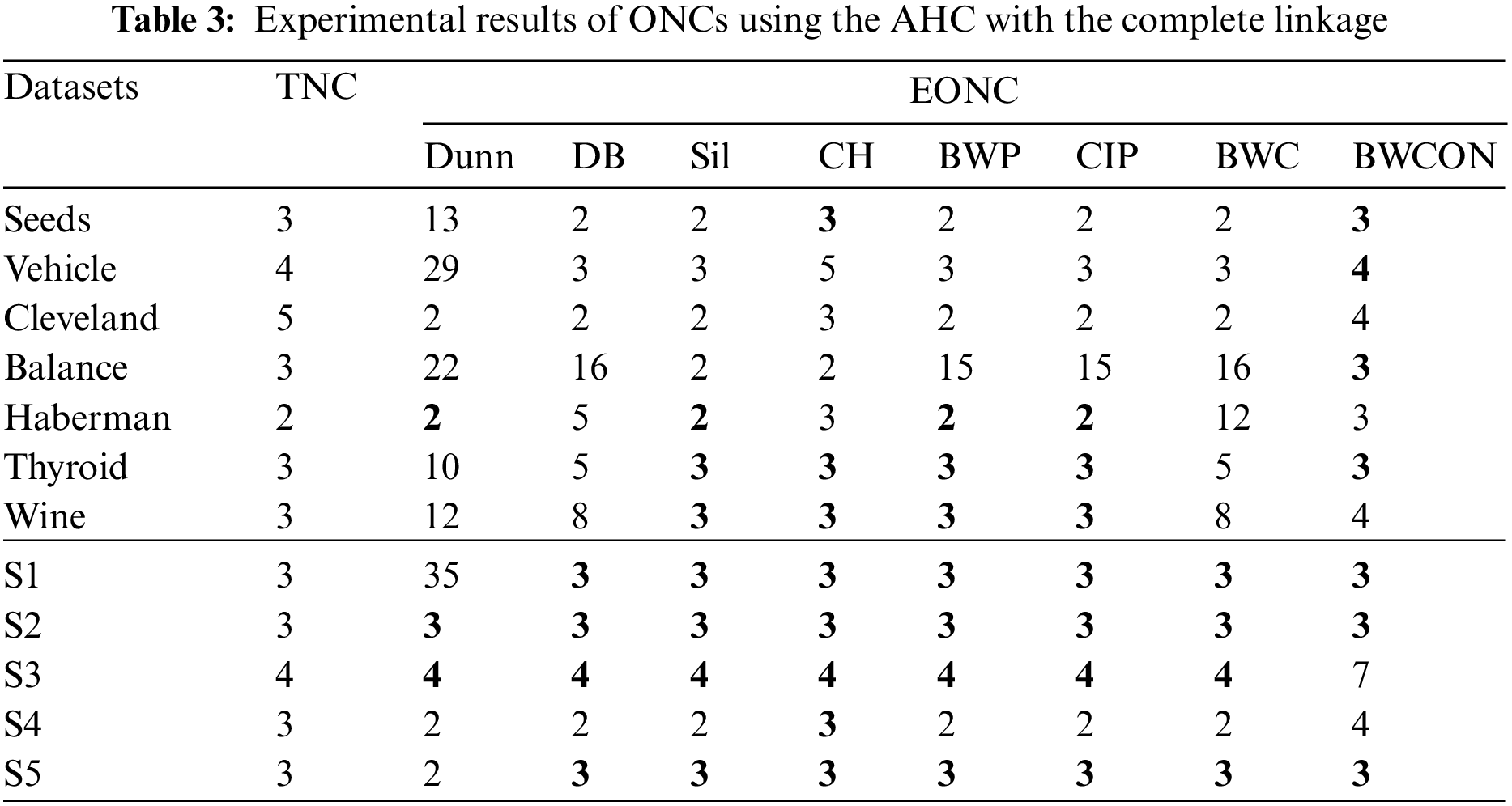
In Table 3, the ONCs estimated by the “BWCON+AHC with the complete linkage”, the “Sil +AHC with the complete linkage” and the “CH+AHC with the complete linkage” are more accurate among all combinations and their estimated biased ONCs are closer to the TNCs. Specifically, for the above 12 datasets, the maximum deviations of the TNCs and the EONCs obtained based on the Dunn, DB, Sil, CH, BWP, CIP, BWC and BWCON are: 32, 13, 3, 2, 12, 12, 13, and 3, respectively. Furthermore, all the above indices are invalid for Cleveland, but the EONC obtained by our index is the closest to the TNC; and only BWCON can obtain the correct NC for Vehicle and Balance datasets.

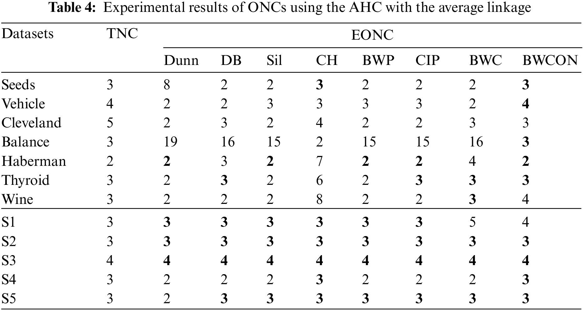
Based on the AHC with the average linkage, the Dunn cannot get the correct NC for six UCI datasets and two synthetic datasets; the DB, Sil and BWP cannot get the correct NC for six UCI datasets and a synthetic dataset; the CH cannot get the correct NC for six UCI datasets; the CIP cannot get the correct NC for five UCI datasets and a synthetic dataset; the BWC cannot get the correct NC for five UCI datasets and two synthetic datasets; and the BWCON cannot get the correct NC only for two UCI datasets and a synthetic dataset. And in Table 4, only BWCON is valid for the Vehicle and Balance, and all the indices are invalid for Cleveland.

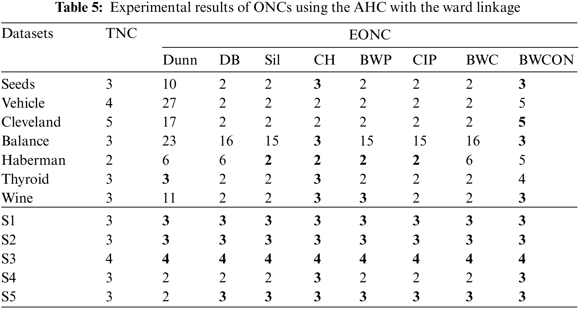
Table 5 shows that the Dunn cannot choose the correct NC for all the twelve datasets except Thyroid, S1, S2 and S3; the DB and BWC are invalid for all the seven UCI datasets and a synthetic dataset; the Sil and CIP are invalid for six UCI datasets and a synthetic dataset; the CH is invalid for Vehicle and Cleveland; the BWP is invalid for six datasets; and the BWCON is invalid for Vehicle, Haberman and Thyroid. It can be seen that combining the BWCON and the CH with the AHC with the ward linkage yield significantly better NC estimation ability than all other combinations. In addition, all the indices cannot obtain the correct NC for Vehicle, and only BWCON can detect the correct NC for Cleveland.

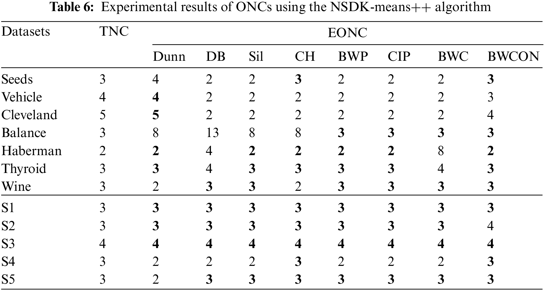
As can be seen from Table 6, the Dunn is invalid for three UCI datasets and two synthetic datasets; the DB cannot get the TNCs for six UCI datasets and one synthetic dataset; the Sil cannot get the TNCs on four UCI datasets and one synthetic dataset; the CH is invalid on four UCI datasets; the BWP and CIP are invalid for three UCI datasets and one synthetic dataset; the BWC is invalid for five UCI datasets and one synthetic dataset; and our proposed BWCON is invalid only on Vehicle, Cleveland and S2. Not only that, further observing the maximum deviations of the TNCs and the EONCs under different indices, it can be seen that for the above 12 datasets, the BWCON has a minimum deviation of only 1, and the other indices, Dunn, DB, Sil, CH, BWP, CIP and BWC, correspond to deviations of 5, 10, 5, 5, 3, 3 and 6, respectively. It is evident that the “BWCON+NSDK-means++” has better NC estimation ability, and the BWCON is more suitable for estimating the NC in combination with our proposed NSDK-means++.

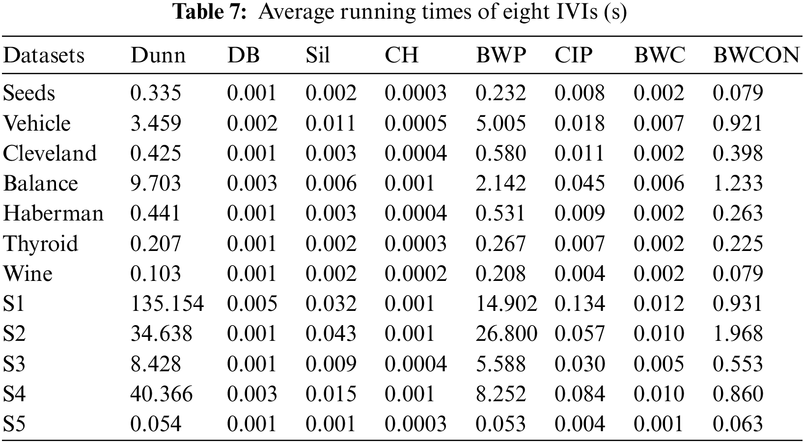
Furthermore, the average running times of eight IVIs on the CPU are presented in Table 7, where to ensure the objectivity of the runtime, we take the average runtime within the search range of each index as the final evaluation value under the NSDK-means++. As shown in Table 7, the time performance of the BWCON is acceptable and it is much faster than the BWP and Dunn indices.

To further support the effectiveness of the BWCON from a statistical point of view, the Friedman test and the Nemenyi test are used [32]. First, to show whether the observed differences of the ability for detecting the TNC among the Dunn, DB, Sil, CH, BWP, CIP, BWC and BWCON are statistically significant, the study conducts the Friedman test for the proposed BWCON and other seven indices on all the experimental datasets in terms of the AHC with the single linkage, complete linkage, average linkage, and ward linkage, and the NSDK-means++ algorithms. For every experimental dataset, the absolute value of the difference between the EONC and the TNC under an index is taken as the final evaluation value; the smaller the evaluation value is, the closer the EONC is to the TNC. Finally, the resulting p-values are 0.000, 0.000, 0.081, 0.000 and 0.162, respectively, revealing that the NC estimation performance of the above eight indices is significantly different under the AHC with the single linkage, complete linkage and ward linkage and there are no significant differences in the NC estimation ability under all indices based on the NSDK-means++ and the AHC with the average linkage, which is likely related to the excellent clustering performance of these two algorithms themselves because the clustering algorithm and the IVI together determine the NC estimation ability, and a good clustering result tends to be more favorable for various IVIs to find the correct NC (the level of test significance is set to 0.05). Then, to further distinguish the performance of each index, the Nemenyi test is performed (the significance level is 0.1) and the obtained critical distance (CD) is 2.78. Where, if the difference between the average order values of the two indices exceeds the CD, the hypothesis that these two indices have the same estimation performance will be rejected; in addition, the smaller the average order value, the better the overall NC estimation ability of the corresponding index on all datasets. Fig. 4 is the Nemenyi test diagram.

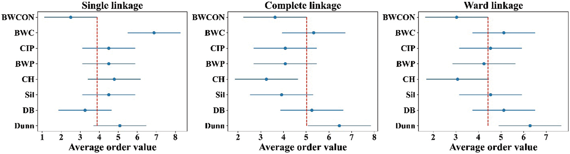
Figure 4: Nemenyi test diagrams under the AHC with the single linkage, complete linkage and ward linkage

In Fig. 4, “·” is the mean ranking score, and the line segment size is CD. For the AHC with the single linkage, the difference between the mean ranking scores of the BWCON and the BWC exceeds the CD, indicating that our proposed BWCON is significantly superior to the BWC in terms of the NC estimation; in addition, compared with all the comparative works, the distribution of “·” corresponding to the BWCON is on the left, which shows that the overall NC estimation ability of the BWCON is better. Similarly, for the AHC with the complete linkage, the NC estimation ability of the BWCON significantly outperforms that of the Dunn, and from the overall NC estimation performance on all datasets, the BWCON beats all indices except the CH but is very close to the CH; and for the AHC with the ward linkage, the BWCON also significantly outperforms the Dunn, and is better than all the comparative indices on the whole as respect to their NC estimation abilities. In general, compared with the other seven popular IVIs, the BWCON has more stable NC estimation ability, and it is easier to be integrated with different clustering algorithms to obtain an accurate NC.

4.3 Performance Evaluation of the BWCON-NSDK-Means++ Algorithm

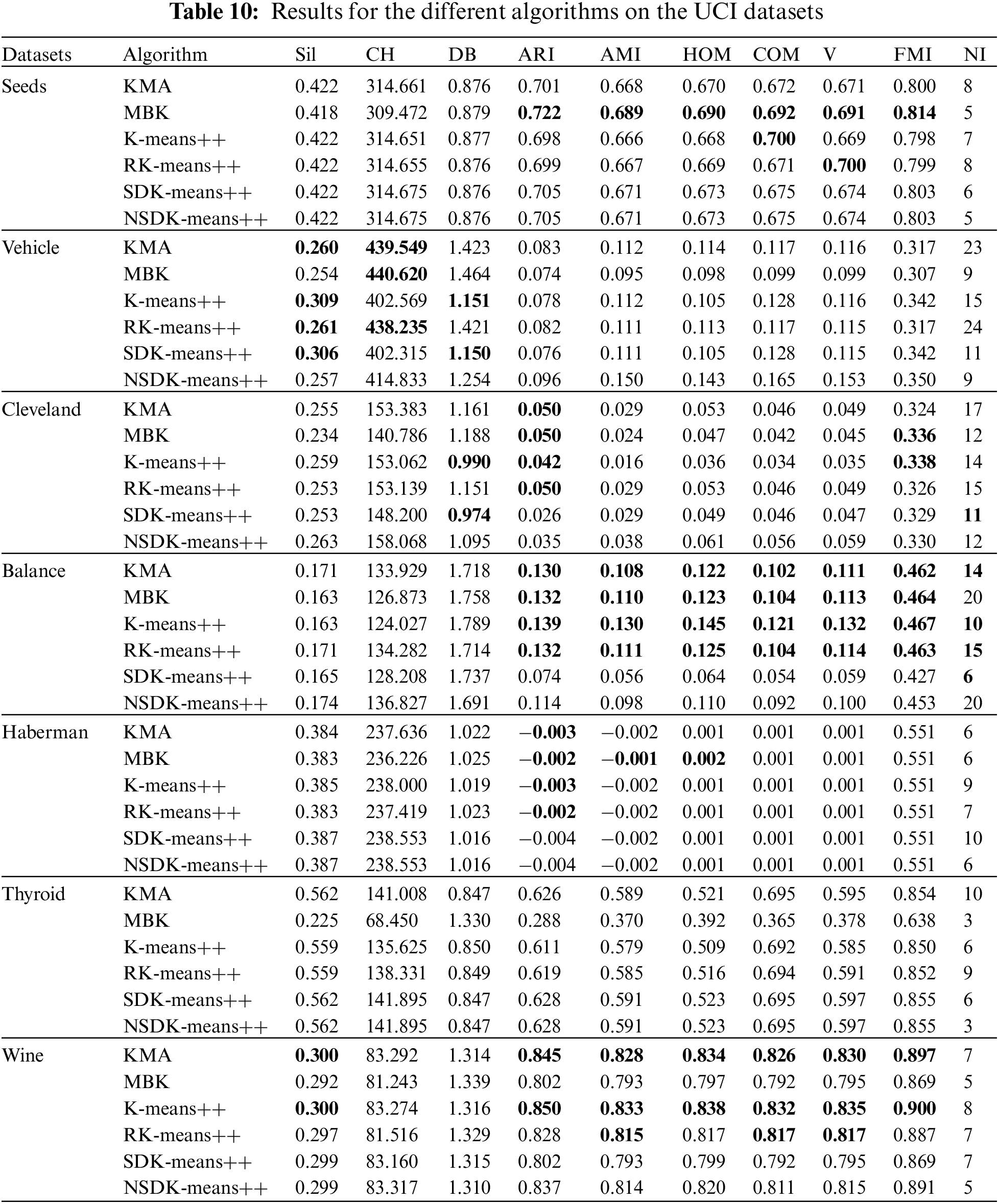
In this section, we conduct experiments to demonstrate the effectiveness of the BWCON-NSDK-means++ in detail from two aspects: (1) to show that the NSDK-means++ itself is a valid clustering algorithm, we focus on comparing the NSDK-means++ and the SDK-means++ since Du et al. [15] have proved that the SDK-means++ is significantly better than the KMA and K-means++ as respect to their clustering performance and speed; and (2) we compare the average ONC accuracies of the “BWCON+NSDK-means++” and nine other combinations to justify that the BWCON-NSDK-means++ is indeed an excellent ONC estimation method. For the first experiment, the results are shown in Tables 8–10; and the second experimental results are shown in Table 11. In addition, since the UCI datasets are usually more complex than those 2-D synthetic datasets, we conduct the first experiment on only UCI datasets; and in terms of the evaluation metrics, to ensure the reliability of the conclusions, we finally adopt three IVIs (i.e., Sil, CH and DB) and six EVIs (i.e., Adjusted Rand Index (ARI), Adjusted Mutual Information (AMI), Homogeneity Score (HOM), Compactness Score (COM), V_measure (V) and Fowlkes and Mallows Index (FMI)) to evaluate the clustering results, which are described in [10,33,34]; except for the DB, all the other indices are found to have the better clustering performance with larger measure values.

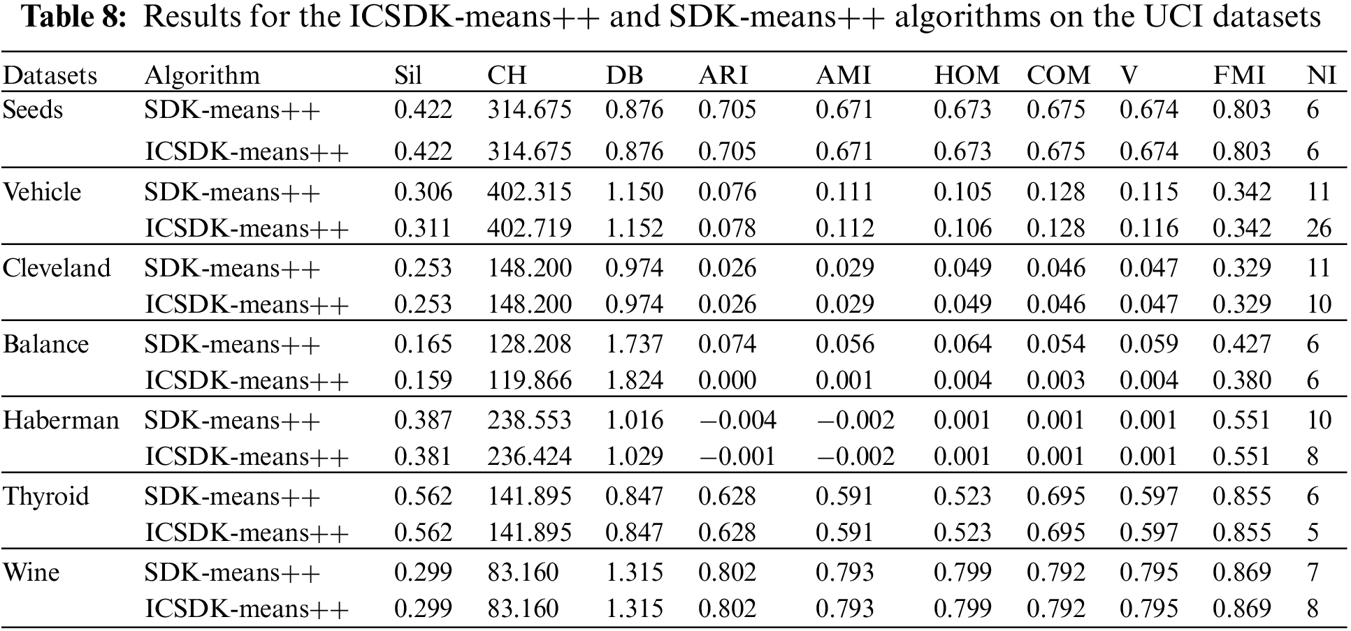
As shown in Table 8, to illustrate that it is feasible to determine the first ICC based on the natural neighbor, we replace the corresponding step in the SDK-means++ and the new algorithm is called ICSDK-means++. From Table 8, we can find that the ICSDK-means++ achieves the comparable or even better clustering performance than the SDK-means++ for all the UCI datasets except Balance, that is to say, the strategy proposed in this study to determine the first ICC without any parameters to be specified is effective. Specifically, on the Seeds, Cleveland, Thyroid and Wine, the ICSDK-means++ has the same clustering performance as the SDK-means++ on nine indices, and the similar NIs; on the Vehicle, although the NI of the ICSDK-means++ is fifteen times more than that of the SDK-means++, the ICSDK-means++ outperforms the SDK-means++ on six indices, achieves the same clustering performance as the SDK-means++ on two indices, and only slightly underperforms the SDK-means++ on one index; on the Haberman, the ICSDK-means++ outperforms the SDK-means++ on one index, achieves the same clustering performance as the SDK-means++ on five indices, and is inferior to the SDK-means++ on three indices, but has two fewer iterations than the SDK-means++.

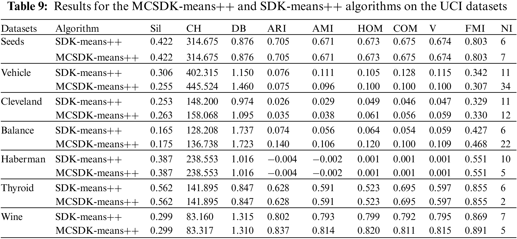
Furthermore, to validate the necessity of modifying the positions of the ICCs in the SDK-means++, we add the modification step to the original SDK-means++, and the new algorithm is denoted as MCSDK-means++. As can be seen from Table 9, except for the Vehicle, the MCSDK-means++ can obtain better clustering results on the remaining six datasets. That is, it is necessary to add the modification step to the SDK-means++. Specifically, on the Seeds, Haberman and Thyroid, the MCSDK-means++ algorithm achieves the same clustering performance as the SDK-means++ on all the indices; for their NIs, except for the Seeds, where the MCSDK-means++ iterates once more than the SDK-means++, in the remaining two datasets, the MCSDK-means++ has fewer iterations than the SDK-means++. On the Clever, the MCSDK-means++ outperforms the SDK-means++ on eight indices; on the Balance, the MCSDK-means++ outperforms the SDK-means++ on all nine indices; and on the Wine, the MCSDK-means++ outperforms the SDK-means++ on eight indices, has the same clustering performance on one index, and has two fewer iterations than the MCSDK-means++.

In addition, Table 10 records the experimental results of the NSDK-means++ and other clustering algorithms; and any evaluation value with better performance than the NSDK-means++ is presented in bold. Besides, for the unstable clustering algorithms (KMA, MBK, K-means++ and RK-means++), we run them 100 times repeatedly and take their average clustering performance as their final evaluation values; particularly, for the MBK, the parameter iteration is equal to the NI of the SDK-means++ on the corresponding dataset, and the mini-batch size is obtained by dividing the dataset size by the NI.

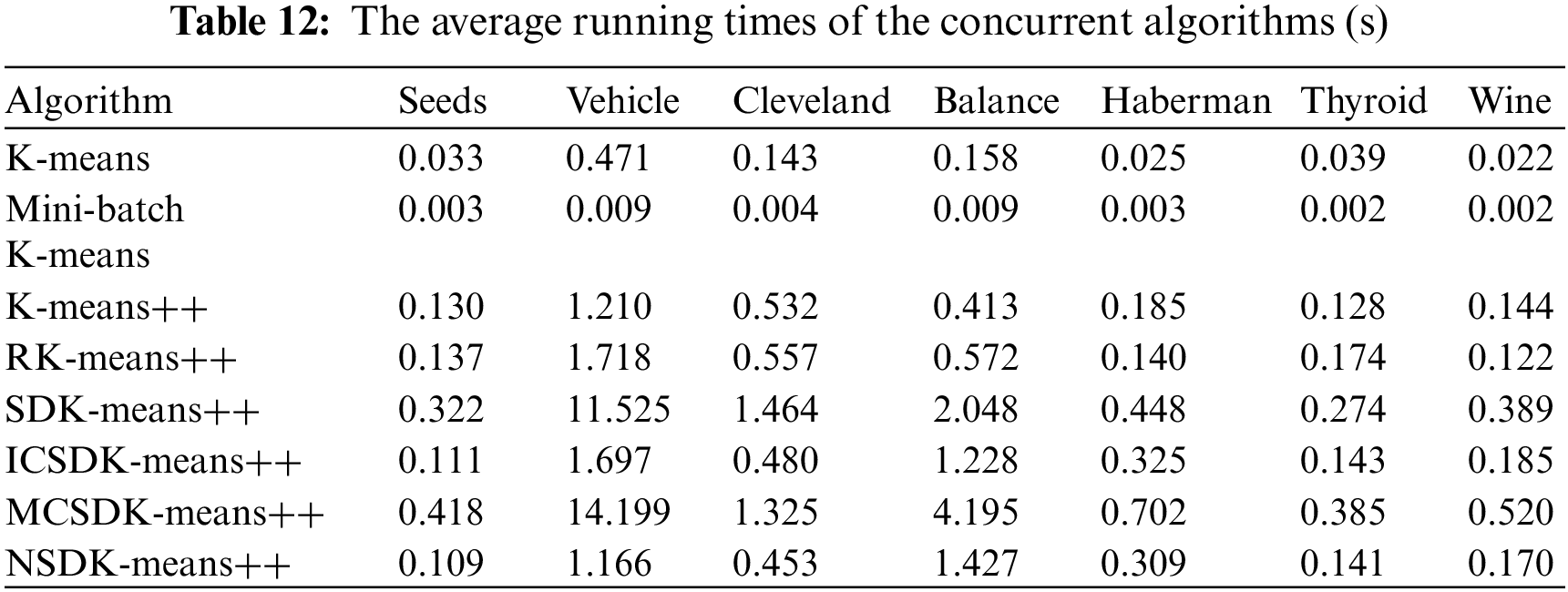
As indicated in Table 10, the proposed NSDK-means++ outperforms the other clustering algorithms on most of the datasets. To better justify our improvements, we focus on the performance differences between the NSDK-means++ and SDK-means++: (1) on the Seeds, the NSDK-means++ has the same clustering performance as the SDK-means++ on nine indices, but in terms of the NI, the NSDK-means++ has one less iteration than the SDK-means++; (2) on the Haberman, the NSDK-means++ has the same clustering performance as the SDK-means++ on nine indices, but the NSDK-means++ has four fewer iterations than the SDK-means++; (3) on the Thyroid, the NSDK-means++ has the same clustering performance as the SDK-means++ on nine indices, but the NSDK-means++ has three fewer iterations than the SDK-means++; (4) on the Vehicle, the NSDK-means++ is superior to the SDK-means++ on seven indices, and iterates two times less than the SDK-Means++; (5) on the Cleveland, although the NSDK-means++ has one more iteration than the SDK-Means++, the NSDK-means++ is superior to the SDK-means++ on eight indices; (6) on the Balance, although the NSDK-means++ iterates fourteen times more than the SDK-means++, the NSDK-means++ is superior to the SDK-means++ on all nine indices; and (7) on the Wine, the NSDK-means++ is superior to the SDK-means++ on eight indices, is comparable to its clustering performance on one index, and has two fewer iterations than the SDK-means++. In particular, our proposed NSDK-means++ achieves good results on the Balance compared with the ICSDK-means++, and also achieves the better results on the Vehicle compared with the MCSDK-means++, which indicate that it is necessary to combine the step of determining the first ICC based on the natural neighbor, the step of determining the remaining ICCs based on the largest sum of distance and the step of modifying the positions of all the ICCs, which can make the obtained ICCs more reasonable and thus improve the overall clustering performance of the SDK-means++. Moreover, shows the average running time of running them 100 times, and the running time of the NSDK-means++ is acceptable.

Not only that, we also further verify the performance differences of the above algorithms from a statistical point of view. Here the resulting p-values using the Friedman test are 0.005, 0.001, 0.003, 0.818, 0.900, 0.713, 0.677, 0.555 and 0.576 respectively as respect to the SC, CH, DB, ARI, AMI, HOM, COM, V and FMI, which show that the performance of the above algorithms is significantly different on the SC, CH and DB (the level of test significance is set to 0.05). Further from Fig. 5, we can find that the NSDK-means++ are significantly superior to the MBK on three indices; moreover, observing the positions of “·”, except that the MCSDK-means++ outperforms the NSDK-means++ on the CH, the NSDK-means++ is not worse than all other algorithms on the whole. Particularly, the performance of the above algorithms does not differ significantly on the six EVIs, which indicates that the NSDK-means++ can achieve a clustering performance comparable to that of those existing algorithms in one run. Here the significance level in the Nemenyi test is 0.1 and CD is 3.640.

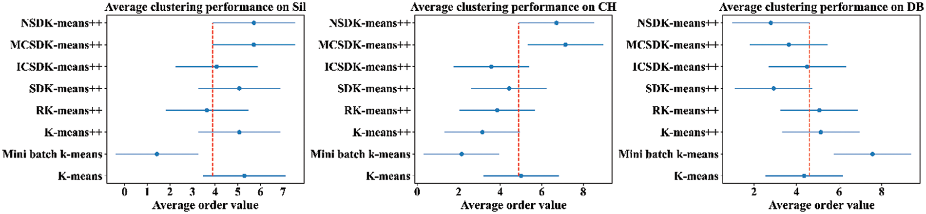
Figure 5: Nemenyi test diagrams for the clustering algorithms

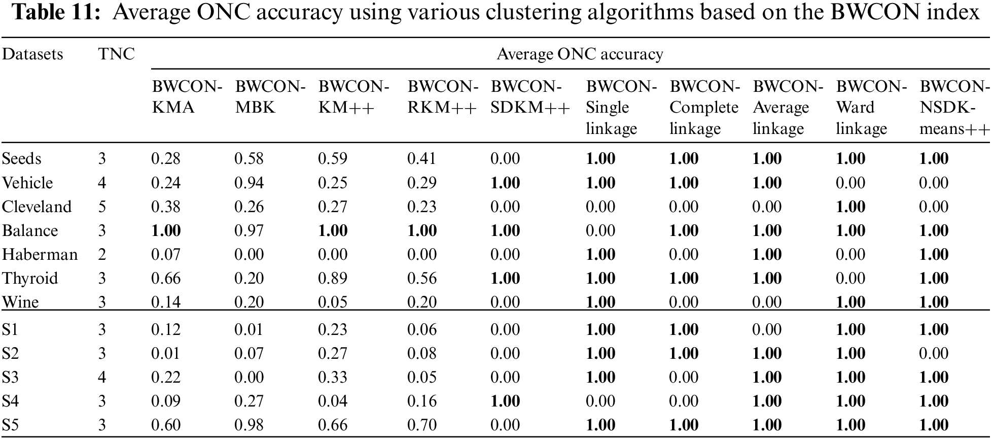
At last, to demonstrate the advantage of the “BWCON+NSDK-means++”, we integrate the KMA, MBK, K-means++, RK-means++, SDK-means++, AHC with the single linkage, AHC with the complete linkage, AHC with the average linkage, AHC with the ward linkage and NSDK-means++ into the proposed BWCON-based ONC estimation framework, respectively, to form the BWCON-KMA, BWCON-MBK, BWCON-KM++, BWCON-RKM++, BWCON-SDKM++, BWCON-Single linkage, BWCON-Complete linkage, BWCON-Average linkage, BWCON-Ward linkage and BWCON-NSDK-means++ to compare their average ONC accuracies (see Eq. (26)), where those unstable clustering algorithms are run 100 times as in [8]. Table 11 lists the results and bold indicates the best performance.

Average ONC accuracy=Number of correct determination of ONC based on acombinationNumber of runs(26)

From Table 11, the BWCON-KMA, BWCON-KM++ and BWCON-RKM++ can achieve an accuracy of 1 only on the Balance; the BWCON-MBK cannot achieve 1 on all datasets, and can only achieve 0.98 on the S5; the BWCON-SDKM++ can obtain an accuracy of 1 on four datasets; the BWCON-Complete linkage can achieve 1 on seven datasets; the BWCON-Single linkage, BWCON-Average linkage, BWCON-Ward linkage and BWCON-NSDK-means++ can achieve an accuracy of 1 on nine datasets. Compared with those existing partition-based clustering algorithms, the NSDK-means++ performs better since it can obtain appropriate ICCs. In addition, although the BWCON-Single linkage, BWCON-Average linkage, BWCON-Ward linkage and BWCON-NSDK-means++ have similar ONC estimation performance in Table 11, the NCs estimated by the algorithm in this paper are closer to the TNCs as shown in Tables 2 and 4–6.

5  Application of the BWCON-NSDK-Means++ in the Market Segmentation

The exact estimation of the ONS serves to achieve an effective market segmentation; and if the obtained sub-markets are not differentiated under a so-called ONS, such market segmentation is not meaningful for an enterprise. From this perspective, we verify the usefulness of the BWCON-NSDK-means++ by analyzing the reasonableness of the corresponding market segmentation results under our ONS. Here, it should be noted that the experiments in this section can be conducted in relation to the fact that the BWCON-NSDK-means++ can also be used as a stand-alone market segmentation tool, which is validated later on the Chinese wine market dataset in 2020.

5.1 Data Collection and Preprocessing

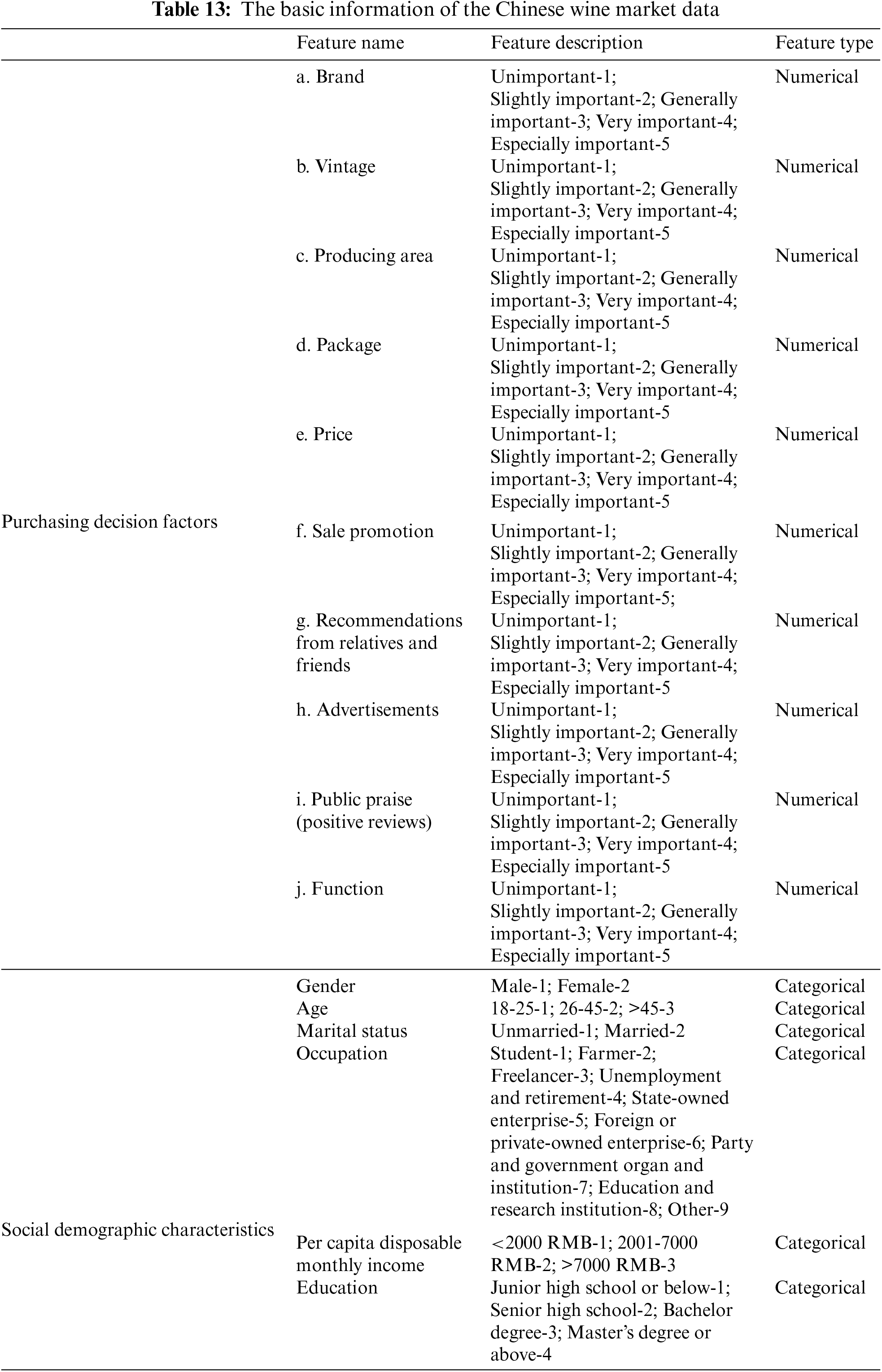
The Chinese wine market dataset in this work is provided by the Chinese Grape Industry Technology System, with a total of 2747 effective samples, including two parts: the factors that affect consumers’ decision-making and the social demographic characteristics as in [5]. The basic information is listed in Table 13 and the first part is presented through the design of Likert five-category attitude scale. Since the wine consumers tend to be younger and more feminine at present, the dataset focuses more on young and well-educated consumers; specifically, the wine consumers under the age of 46 account for 85.7%, and those with a bachelor’s degree or above account for 86.8%.

In our study, to facilitate the analysis of the practical implications of the market segmentation results, we choose the first part as the market segmentation bases (SB). Moreover, to remove the relevance among the SB, we adopt the Exploratory Factor Analysis (EFA) [35] to deal with them, and after statistical analysis, the KMO value is 0.840, the approximate Chi-Square value in the Bartlett’s sphere test is 6479.893, and it is significant at the level of 0.000, which verifies that the dataset is suitable for the EFA. Thus ultimately, we identify four SB to participate in this segmentation task based on the following principles: the cumulative variance contribution rate is greater than 60%, the extraction degrees of the factors are all greater than 0.5, the factor loading values are all greater than 0.6 and each common factor represents at least two factors, as shown in Fig. 6.

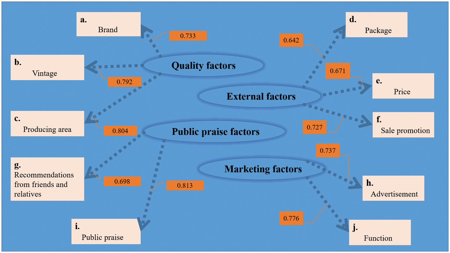
Figure 6: Factor loading diagram of four SB

5.2 Determination of the ONS

In this section, based on the above four SB, the BWCON-NSDK-means++ is used to detect the ONS, as shown in Fig. 7. We can find that for the compactness, when the NC changes from 3 to 4, the fluctuation is maximum and positive, thus according to Eq. (17), ncom = 4; for the separation, when the NC changes from 2 to 3, a positive maximum fluctuation can be obtained, so according to Eq. (18), nsep = 3; and finally, for the connectivity, a negative maximum fluctuation can be found when the NC changes from 2 to 3, thus according to Eq. (19), ncon = 2. Eventually, we can obtain that the ONS is 3 based on the Eq. (20), which is following the finding of [36].

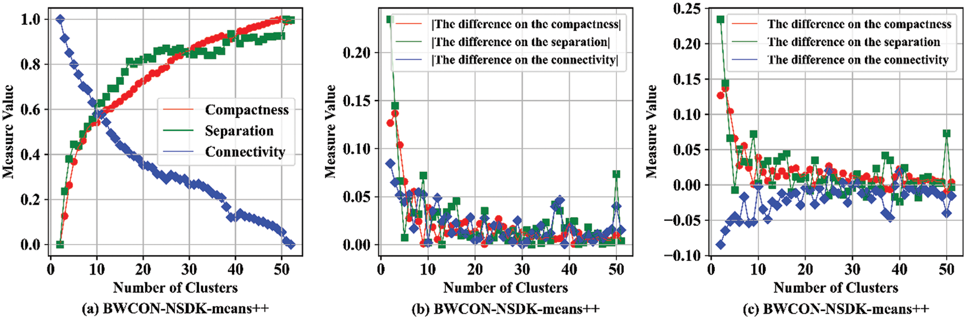
Figure 7: The determination of the ONS based on the BWCON-NSDK-means++

Furthermore, to verify the reliability of the ONS obtained above, we further detect the corresponding ONSs using the BWCON-Single linkage, BWCON-Average linkage and BWCON-Ward linkage mentioned in Section 4.3, as shown in Fig. 8. It can be found that all these algorithms consider segmenting the Chinese wine market into three sub-markets as the best, which indicates that the ONS determined based on the BWCON-NSDK-means++ is indeed reliable.

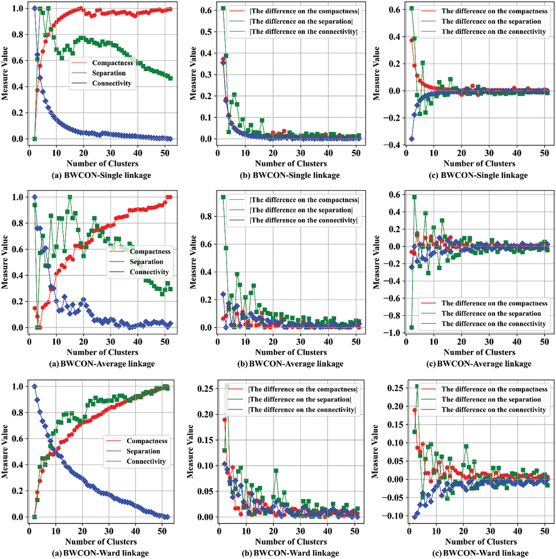
Figure 8: The determination of the ONS based on the BWCON-Single linkage, BWCON-Average linkage and BWCON-Ward linkage algorithms

5.3 The Practicality Analysis of the BWCON-NSDK-Means++ Algorithm

To check the rationality of the market segmentation results under our obtained ONS and the effectiveness of the BWCON-NSDK-means++ as an independent market segmentation tool, we compare the market segmentation results of the BWCON-Single linkage, BWCON-Average linkage, BWCON-Ward linkage and BWCON-NSDK-means++ as respect to the inter-market differentiation, sub-market size and consumer group characteristics, as shown in Tables 14 and 15, and Figs. 9 and 10.

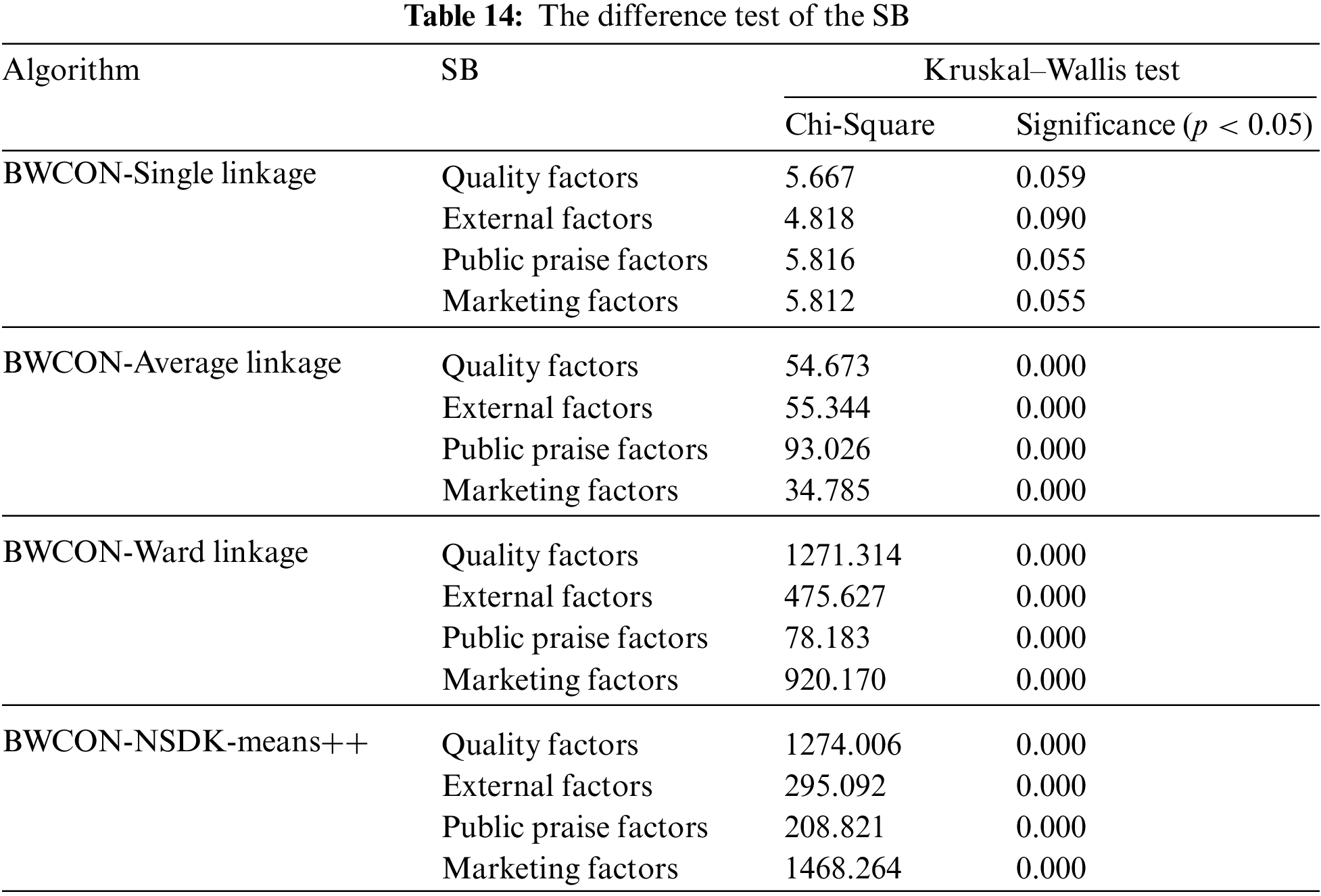
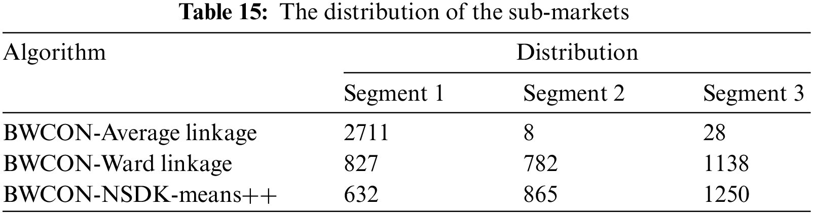
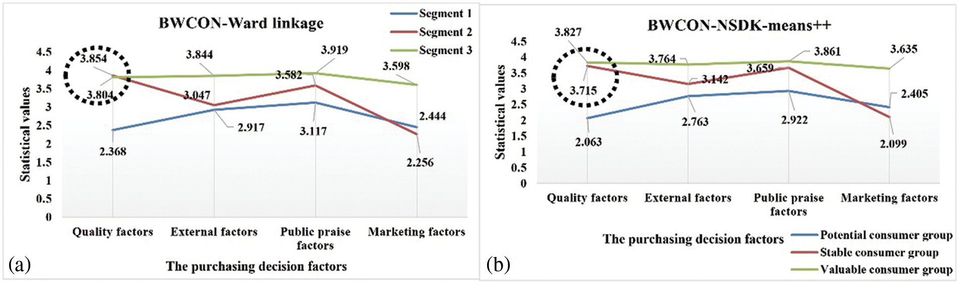
Figure 9: Visualization of segments on the SB

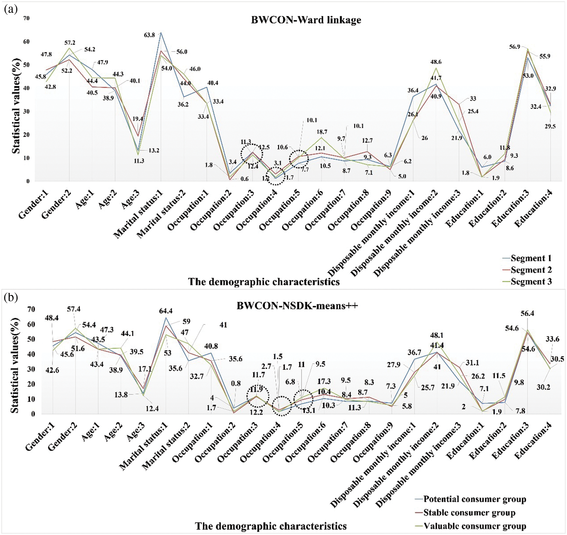
Figure 10: Visualization of segments on the demographic characteristics

Table 14 tabulates the results of the Kruskal-Wallis test. Except for the BWCON-Single linkage, the p-values corresponding to the remaining three algorithms are all less than 0.05, which indicate that there are significant differences on the SB among the three sub-markets obtained by the BWCON-Average linkage, BWCON-Ward linkage and BWCON-NSDK-means++. Based on this, we further summarize the sub-market sizes corresponding to these three algorithms in Table 15; and for the distribution, we adopt the view of Kotler et al. [37], i.e., any given sub-market is worthy of further analysis only if it contains at least 5% of all the consumers, and it is 138 here. Thus it can be seen that for the BWCON-Average linkage, although there are differences among the different segments, the sub-market sizes of both Segments 2 and 3 are significantly smaller than 138, which are of no research value to the enterprises; on the contrary, the sub-market scales of the BWCON-Ward linkage and BWCON-NSDK-means++ are both larger than 138, and their distributions are similar, which may have something to do with the fact that the AHC with the ward linkage itself is an excellent market segmentation tool [38].

Given the informative value of the market segmentation results derived from the BWCON-Ward linkage, we compare the consumption preferences and consumer characteristics of all the sub-markets obtained using the BWCON-Ward linkage and BWCON-NSDK-means++ to illustrate the robustness of the conclusions obtained by the BWCON-NSDK-means++ in Figs. 9 and 10, respectively, where for the SB, the mean value of each feature is taken as the statistical value, and for the demographic characteristics, the frequency share of each feature is taken as the final statistical value.

As shown in Fig. 9, the wine consumers in the “Segment 1” and “Potential consumer group” have completely similar consumption psychologies: Public praise factors > External factors > Marketing factors > Quality factors; similarly, both “Segment 2” and “Stable consumer group” are characterized by the same consumption tendencies: Quality factors > Public praise factors > External factors > Marketing factors; and as for the remaining two sub-markets, their consumer preferences are also only slightly different, e.g., in the “Segment 3”, the relationship among different SB is Public praise factors > External factors > Quality factors > Marketing factors, and in the “Valuable consumer group”, the relationship is Public praise factors > Quality factors > External factors > Marketing factors. That is to say, the purchasing psychologies derived using these two algorithms are basically identical. Not only that, from Fig. 10, except for the Occupations 1, 3, 4 and 5, and Education 3, the distributions of the demographic characteristics in our “Potential consumer group”, “Stable Consumer Group”, and “Valuable consumer group” are fully consistent with those in the “Segment 1”, “Segment 2” and “Segment 3”, respectively. Therefore, the conclusions provided by our method are robust and reliable, and the BWCON-NSDK-means++ is also indeed a qualified market segmentation tool.

5.4 Results of the Chinese Wine Market Segmentation

In this section, to have a better understanding of the practical meanings of our obtained market segmentation results based on the BWCON-NSDK-means++, we visualize each sub-market in Fig. 11, in which the black dots represent the characteristics of the entire Chinese wine market, and for each sub-market, the numerical variables have the mean as the statistical object, and the categorical variable has the frequency share as the statistical object.

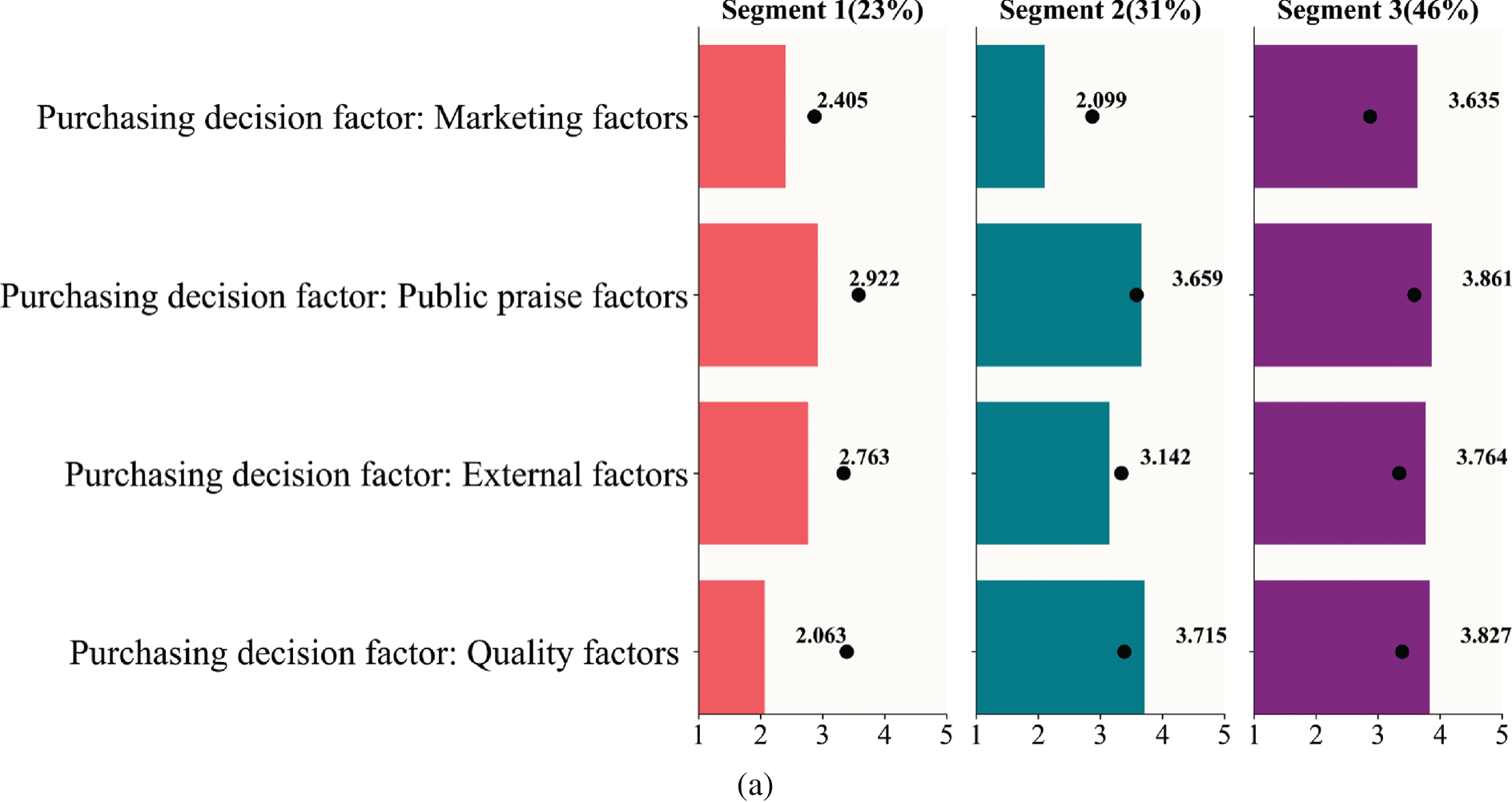
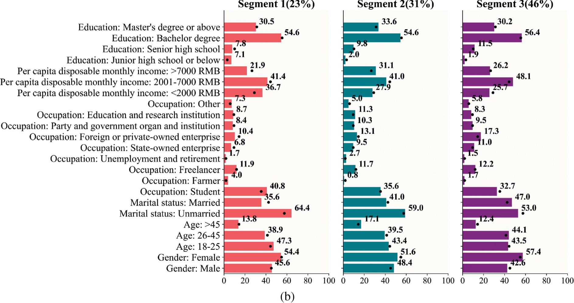
Figure 11: Visualization of segments based on the BWCON-NSDK-means++: (a) Differences on the SB; (b) Differences on the demographic characteristics

Segment 1: Potential consumer group (23%). This is the smallest of the segments. Compared with the other two consumer groups, this group has the largest share of young unmarried consumers (47.3% are 18–25 years old) and more students, farmers and other occupations. In particular, the students account for 40.8% of the total consumer group, making this consumer group the one with the lowest per capita disposable monthly income of the three consumer groups (i.e., the disposable income per month of 36.7% consumers is less than 2000 RMB). In term of education, maybe since the percentage of farmers is slightly higher than the other two groups, there are slightly more consumers with junior high school education or below, but within the group, 54.6% consumers have a bachelor’s degree. For this young group, the concern for wine quality, external factors, public praise factors and marketing factors is lower than the average level of the whole market, but inside the sub-market, this group cares more about the public praise and external factors of the wine. Therefore, if an enterprise plans to choose this sub-market as its target market, it can improve its public praise or change the price, package, etc. to increase consumers’ satisfaction.

Segment 2: Stable consumer group (31%). This is the second largest segment. Among the three consumer groups, this group has the largest proportion of elderly male consumers (17.1% of consumers are over 46 years old), and because of this, the proportion of the leavers and retirees in this group is higher than the other two groups (i.e., 2.7% of consumers have left their jobs or retired). In addition, for the occupation, the shares of employees come from Party and government organ (10.3%) and in education and research institutions (11.3%) are also higher than them in the other two groups. At the same time, this is a high-income and highly educated group; 31.1% of consumers have a per capita disposable monthly income above 7000 RMB, and 33.6% of consumers are with master’s degree or above. Within the market, the consumers care most about the quality of the wine when purchasing wine; therefore, improving the quality of wine can increase the satisfaction of this consumer group.

Segment 3: Valuable consumer group (46%). This is the largest segment. In this consumer group, there are more married middle-aged female consumers than in the other two groups (i.e., 57.4% of consumers are female, 44.1% are 26–45 years old); and freelancers, state, foreign and private employees account for a higher proportion than the other two groups. This is a middle-income consumer group (i.e., 48.1% of consumers have a per capita disposable monthly income of 2001–7000 RMB), and consumers with senior high school or bachelor degrees are higher than the other two groups. This group is more concerned with the quality, external factors (i.e., price, package, etc.), public praise and marketing factors; in particular, if an enterprise chooses this sub-market as its target market, improving the public praise of the wine can significantly increase consumers’ satisfaction.

6  Conclusions and Future Work

It is a premise to set a reasonable ONS to carry out a successful market segmentation, however, in the current research, there is a serious lack of attention to this issue. In our study, we propose such a method called BWCON-NSDK-means++ to adaptively determine the ONS by effectively integrating a new IVI and a valid clustering algorithm into a novel ONS estimation framework. Specifically, inspired by the neighboring samples, a connectivity formula is quantitatively defined for the first time, and thus the BWCON is designed to comprehensively evaluate the market segmentation results from three perspectives: compactness, separation and connectivity. Then, a BWCON-based ONS estimation framework is innovatively constructed by elegantly trade-off the ONCs from the three evaluation dimensions. Finally, the BWCON-NSDK-means++ is obtained by integrating our improved NSDK-means++ into the aforementioned ONS estimation framework. The final experimental results show that compared with those existing models, the BWCON and NSDK-means++ are more suitable to be combined to determine the ONC. Moreover, the experiments on the Chinese wine market dataset in particular prove that the BWCON-NSDK-means++ is not only an effective ONS estimation method, but also a qualified market segmentation tool without extra parameters; and it can help relevant practitioners understand a market more objectively and thus make more correct and valuable decisions.

Experiments have demonstrated the power of the BWCON-NSDK-means++, but there are still some shortcomings to be further optimized, such as the choice of the clustering algorithm used in the combination. In the present study, we choose the partition-based NSDK-means++ to integrate with the BWCON mainly due to its stability and the fact that only one parameter NC needs to be set, but we ignore its limitation that the partitioning clustering itself is more suitable for spherical datasets. Therefore, as a future direction, we will further optimize the NSDK-means++ to make the combination “BWCON+NSDK-means++” more widely applicable.

Funding Statement: This study was supported by the earmarked fund for CARS-29 and the open funds of the Key Laboratory of Viticulture and Enology, Ministry of Agriculture, China.

Availability of Data and Materials: The Seeds, Vehicle, Cleveland, Balance, Haberman, Thyroid and Wine are the public datasets, and they are available in the UCI Machine Learning Repository (http://archive.ics.uci.edu/ml/). The S1, S2 and S3 are generated by using the “multivariate_normal” function from the numpy. The S4 and S5 are generated using the “make_blobs” function of the sklearn. And the Chinese wine market dataset is available on request from the corresponding author.

Conflicts of Interest: The authors declare that we have no conflicts of interest to report regarding the present study.

References

1. Chang, Y. T., Fan, N. H. (2022). A novel approach to market segmentation selection using artificial intelligence techniques. The Journal of Supercomputing, 22(2), 79. https://doi.org/10.1007/s11227-022-04666-2 [Google Scholar] [CrossRef]

2. Casas-Rosal, J. C., Segura, M., Maroto, C. (2021). Food market segmentation based on consumer preferences using outranking multicriteria approaches. International Transactions in Operational Research, 30(3), 1537–1566. https://doi.org/10.1111/itor.12956 [Google Scholar] [CrossRef]

3. Seo, H. (2021). Dual’ labour market? Patterns of segmentation in European labour markets and the varieties of precariousness. Transfer: European Review of Labour and Research, 27(4), 485–503. https://doi.org/10.1177/10242589211061070 [Google Scholar] [CrossRef]

4. Wang, H. J. (2022). Market segmentation of online reviews: A network analysis approach. International Journal of Market Research, 64(5), 652–671. https://doi.org/10.1177/14707853211059076 [Google Scholar] [CrossRef]

5. Qi, J., Li, Y., Jin, H., Feng, J., Mu, W. (2022). User value identification based on an improved consumer value segmentation algorithm. Kybernetes, 13(3), 233. https://doi.org/10.1108/K-01-2022-0049 [Google Scholar] [CrossRef]

6. Abbasimehr, H., Bahrini, A. (2022). An analytical framework based on the recency, frequency, and monetary model and time series clustering techniques for dynamic segmentation. Expert Systems with Applications, 192(4), 116373. https://doi.org/10.1016/j.eswa.2021.116373 [Google Scholar] [CrossRef]

7. Zhou, S., Liu, F., Song, W. (2021). Estimating the optimal number of clusters via internal validity index. Neural Processing Letters, 53(2), 1013–1034. https://doi.org/10.1007/s11063-021-10427-8 [Google Scholar] [CrossRef]

8. Abdalameer, A. K., Alswaitti, M., Alsudani, A. A., Isa, N. A. M. (2022). A new validity clustering index-based on finding new centroid positions using the mean of clustered data to determine the optimum number of clusters. Expert Systems with Applications, 191, 116329. https://doi.org/10.1016/j.eswa.2021.116329 [Google Scholar] [CrossRef]

9. Tavakkol, B., Choi, J., Jeong, M. K., Albin, S. L. (2022). Object-based cluster validation with densities. Pattern Recognition, 121, 108223. https://doi.org/10.1016/j.patcog.2021.108223 [Google Scholar] [CrossRef]

10. Naderipour, M., Zarandi, M. H. F., Bastani, S. (2022). A fuzzy cluster-validity index based on the topology structure and node attribute in complex networks. Expert Systems with Applications, 187(1), 115913. https://doi.org/10.1016/j.eswa.2021.115913 [Google Scholar] [CrossRef]

11. Zhou, S., Liu, F. (2022). A novel internal cluster validity index. Journal of Intelligent & Fuzzy Systems, 38(4), 4559–4571. https://doi.org/10.3233/JIFS-191361 [Google Scholar] [CrossRef]

12. He, H., Zhao, Z., Luo, W., Zhang, J. (2021). Community detection in aviation network based on K-means and complex network. Computer Systems Science and Engineering, 39(2), 251–264. https://doi.org/10.32604/csse.2021.017296 [Google Scholar] [CrossRef]

13. Sheikhhosseini, Z., Mirzaei, N., Heidari, R., Monkaresi, H. (2021). Delineation of potential seismic sources using weighted K-means cluster analysis and particle swarm optimization (PSO). Acta Geophysica, 69(6), 2161–2172. https://doi.org/10.1007/s11600-021-00683-6 [Google Scholar] [CrossRef]

14. Wu, G., Zhang, D., Fan, S. (2022). Application of an improved K-means clustering algorithm in power user grouping. International Journal of Numerical Modelling: Electronic Networks, Devices and Fields, 35(4). https://doi.org/10.1002/jnm.2990 [Google Scholar] [CrossRef]

15. Du, G., Li, X., Zhang, L., Liu, L., Zhao, C. (2021). Novel automated K-means++ algorithm for financial data sets. Mathematical Problems in Engineering,2021,1–12. https://doi.org/10.1155/2021/5521119 [Google Scholar] [CrossRef]

16. Dunn, J. C. (1973). A fuzzy relative of the ISODATA process and its use in detecting compact well-separated clusters. Journal of Cybernetics, 3(3), 32–57. https://doi.org/10.1080/01969727308546046 [Google Scholar] [CrossRef]

17. Davies, D. L., Bouldin, D. W. (1979). A cluster separation measure. IEEE Transactions on Pattern Analysis and Machine Intelligence, PAMI-1(2), 224–227. https://doi.org/10.1109/TPAMI.1979.4766909 [Google Scholar] [CrossRef]

18. Rousseeuw, P. J. (1987). Silhouettes: A graphical aid to the interpretation and validation of cluster analysis. Journal of Computational and Applied Mathematics, 20(87), 53–65. https://doi.org/10.1016/0377-0427(87)90125-7 [Google Scholar] [CrossRef]

19. Calinski, T., Harabasz, J. (1974). A dendrite method for cluster analysis. Communications in Statistics-Simulation and Computation, 3(1), 1–27. https://doi.org/10.1080/03610917408548446 [Google Scholar] [CrossRef]

20. Zhou, S., Xu, Z., Tang, X. (2011). Method for determining optimal number of clusters based on affinity propagation clustering. Control and Decision, 26(8), 7. [Google Scholar]

21. Dogan, A., Birant, D. (2022). K-centroid link: A novel hierarchical clustering linkage method. Applied Intelligence, 52(5), 5537–5560. https://doi.org/10.1007/s10489-021-02624-8 [Google Scholar] [CrossRef]

22. Mahdi, M. A., Hosny, K. M., Elhenawy, I. (2021). Scalable clustering algorithms for big data: A review. IEEE Access, 9, 80015–80027. https://doi.org/10.1109/access.2021.3084057 [Google Scholar] [CrossRef]

23. Chan, C., Al-Bashabsheh, A., Zhou, Q. (2021). Agglomerative info-clustering: Maximizing normalized total correlation. IEEE Transactions on Information Theory, 67(3), 2001–2011. https://doi.org/10.1109/TIT.2020.3040492 [Google Scholar] [CrossRef]

24. Banerjee, P., Chakrabarti, A., Ballabh, T. K. (2021). Accelerated single linkage algorithm using the farthest neighbour principle. Sādhanā, 46(1), 45. https://doi.org/10.1007/s12046-020-01544-6 [Google Scholar] [CrossRef]

25. Tokuda, E. K., Comin, C. H., Costa, L. (2022). Revisiting agglomerative clustering. Physica A: Statistical Mechanics and its Applications, 585(3), 126433. https://doi.org/10.1016/j.physa.2021.126433 [Google Scholar] [CrossRef]

26. Sinaga, K. P., Yang, M. S. (2020). Unsupervised K-means clustering algorithm. IEEE Access, 8, 80716–80727. https://doi.org/10.1109/ACCESS.2020.2988796 [Google Scholar] [CrossRef]

27. Sculley, D. (2010). Web-scale k-means clustering. Proceedings of the 19th International Conference on World Wide Web-WWW '10. https://doi.org/10.1145/1772690.1772862 [Google Scholar]

28. Fahim, A. (2021). K and starting means for K-means algorithm. Journal of Computational Science, 55(1), 1011445. https://doi.org/10.1016/j.jocs.2021.101445 [Google Scholar] [CrossRef]

29. Arthur, D., Vassilvitskii, S. (2007). K-means++: The advantages of careful seeding. Proceedings of the Eighteenth Annual ACM-SIAM Symposium on Discrete Algorithms, pp. 1027–1035. New Orleans, Louisiana. [Google Scholar]

30. Zhang, M., Duan, K. F. (2015). Improved research to K-means initial cluster centers. Ninth International Conference on Frontier of Computer Science and Technology, pp. 349–353. https://doi.org/10.1109/fcst.2015.61 [Google Scholar] [CrossRef]

31. Zhu, Q., Feng, J., Huang, J. (2016). Natural neighbor: A self-adaptive neighborhood method without parameter K. Pattern Recognition Letters, 80(1), 30–36. https://doi.org/10.1016/j.patrec.2016.05.007 [Google Scholar] [CrossRef]

32. Li, Y., Chu, X., Tian, D., Feng, J., Mu, W. (2021). Customer segmentation using K-means clustering and the adaptive particle swarm optimization algorithm. Applied Soft Computing, 113(1), 107924. https://doi.org/10.1016/j.asoc.2021.107924 [Google Scholar] [CrossRef]

33. Qaddoura, R., Faris, H., Aljarah, I. (2020). An efficient clustering algorithm based on the k-nearest neighbors with an indexing ratio. International Journal of Machine Learning and Cybernetics, 11(3), 675–714. https://doi.org/10.1007/s13042-019-01027-z [Google Scholar] [CrossRef]

34. Shi, J., Ye, L., Li, Z., Zhan, D. (2022). Unsupervised binary protocol clustering based on maximum sequential patterns. Computer Modeling in Engineering & Sciences, 130(1), 483–498. https://doi.org/10.32604/cmes.2022.017467 [Google Scholar] [CrossRef]

35. Maciejewski, G., Mokrysz, S., Wróblewski, Ł. (2019). Segmentation of coffee consumers using sustainable values: Cluster analysis on the polish coffee market. Sustainability, 11(3), 613. https://doi.org/10.3390/su11030613 [Google Scholar] [CrossRef]

36. Mu, W., Zhu, H., Tian, D., Feng, J. (2017). Profiling wine consumers by price segment: A case study in Beijing, China. Italian Journal of Food Science, 29(3), 377–397. [Google Scholar]

37. Kotler, P., Stewart, A., Linden, B., Armstrong, G. (2001). Principles of marketing. Frenchs Forest: Pearson Education Australia. [Google Scholar]

38. Kaliji, S. A., Imami, D., Gjonbalaj, M., Canavari, M., Gjokaj, E. (2022). Fruit-related lifestyles as a segmentation tool for fruit consumers. British Food Journal, 124(13), 126–142. https://doi.org/10.1108/BFJ-09-2021-1001 [Google Scholar] [CrossRef]