Residential Energy Consumption Forecasting Based on Federated Reinforcement Learning with Data Privacy Protection

1  Introduction

In recent years, global energy consumption [1–3] has been increasing rapidly due to economic development and population increase, which exacerbates the shortage of natural resources and global temperature increase. Consequently, it is essential to improve energy efficiency and to make energy predictable. This is crucial for the construction industry’s “double carbon” goal [4,5]. Smart grids are also widely used as a result of the rapid development of information technology and artificial intelligence technology. The Advanced Metering Infrastructure (AMI) [6], which can collect power usage data from customers instantly or at regular intervals, is a major part of the smart grid. The data is shown as a time series. And we can collect a lot of time series data, which is very useful for researching energy forecasting.

After investigating a substantial amount of literature, we discover that there are approximately three major categories of methodologies for predicting energy consumption: engineering methods, statistical methods, and machine learning methods. The first two methods are traditional prediction methods. Machine learning methods utilizing big data for training calculations make it possible to make energy predictions quickly and easily.

Compared to the other two types of methods, engineering methods are not user-friendly and difficult to understand. This is because these methods use physical principles and thermodynamic equations to calculate the energy consumption of building components. In general, obtaining detailed building and environmental information is more difficult. This is because it uses physical principles and thermodynamic formulas to calculate the energy consumption of each component in a building. In general, it is more difficult to obtain detailed building and environmental information. In 2006, Wang et al. [7] proposed a simplified building thermal model for energy prediction, which is based on frequency patterns analysis to obtain the parameters of a simplified model of the building envelope, using a thermal network to represent the internal mass of the building, but the prediction results are less perfect because this method used a simplified model. Following the introduction of statistical methods, the process of calculating energy forecasts became more intuitive and faster. It uses mathematical formulas to link data on building energy consumption to influencing factors. In 2010, Ma et al. [8] developed an integrated model for energy forecasting based on multiple linear regression and autoregression. They analyzed the electricity consumption data of large public buildings in Xi’an city and chose the least squares algorithm for parameter estimation, then predicted the electricity consumption trend in public buildings. Hong et al. [9] proposed two different methods for forecasting energy consumption in the residential sector. The model they proposed achieved better forecasting performance. However, the high requirements of the method in terms of input information, simulation techniques and calculations prevented its widespread use.

The development of machine learning methods has resulted in much higher accuracy in predicting energy consumption. Decision Trees (DT), Support Vector Machines (SVM), Artificial Neural Networks (ANN), and other traditional machine learning methods are examples. Guo et al. [10] used SVM to forecast future electricity demand in 2017. Ekonomou [11] proposed the multilayer perceptron model (MLP) approach for energy forecasting and compared it with SVM and linear regression models. The experimental results show that MLP performs better in prediction. Hou et al. [12] proposed the support vector machine (SVM) model. Using this neural network algorithm to predict the cooling load of heating, ventilation and air conditioning (HVAC) systems, the results show that the support vector machine method performs better compared to the autoregressive integrated moving average (ARIMA) method. Subsequently, Yaslan et al. [13] developed the EMD-SVR model, which combines support vector regression (SVR) and empirical mode decomposition (EMD) algorithms for electricity load demand forecasting, and the results showed that the model outperformed SVR and non-feature use denoising SVR algorithms for forecasting. In 2015, Sajjad et al. [14] proposed a radial basis function (RBF) neural network model for short-term load forecasting based on a novel stochastic search algorithm and compared its prediction results to the MLP network. Agatonovic-Kustrin et al. [15] developed an artificial neural network (ANN) technique for estimating and forecasting future industrial energy demand in the United States and compared it with multiple linear regression (MLR) model, concluding that the artificial neural network technique is a very promising technique for the future. Deep learning [16,17] is commonly used for load prediction, and neural networks outperform other prediction methods.

Brunke et al. [18] proposed a combined recurrent neural network (RNN) and convolutional neural network (CNN) approach for building load prediction in 2019, which was compared with the seasonal ARIMAX model in terms of accuracy, computational efficiency, and generality, and the prediction accuracy was greatly improved. In 2020, Guo et al. [19] proposed a multi-scale CNN-LSTM hybrid neural network with inputs of historical energy consumption data, real-time electricity price, and weather factors, followed by short-term load prediction using convolutional neural network (CNN) and long and short-term memory (LSTM), and experiments demonstrated that this model has high prediction accuracy and application value. Ozcan et al. [20] proposed a novel deep learning method based on a two-stage attentional recurrent neural network to predict electric load consumption in 2021. For feature extraction, the method employs an encoder and a decoder as well as an attention mechanism. The experimental results show that the method performs better than other methods.

Artificial intelligence technology is now widely used in a variety of fields. We have read a wide range of research and reviews of extensive literature [21–31] and find that most studies have experimented with predicting energy consumption by pooling data for model training. However, the process of centralizing data can result in data leakage. In the construction industry, a data breach could reveal the number of occupants in a household, the location of the family home, and whether or not the occupants are present. The leakage of this private data poses a risk to households.

At the same time, many laws and regulations on data security and privacy have been enacted, making it difficult to centralize data, which can lead to a data silo problem, in which data is not allowed to be shared among different users. To train the model while protecting the privacy of the users, Yang et al. [21] proposed federated learning, which is a distributed machine learning method. It trains the model collaboratively by multiple users while keeping each household’s data present locally and uploading only the encrypted parameters to participate in the global model’s secure aggregation. As a result, federated learning leverages distributed resources for efficient machine learning while also providing raw data security and privacy. The FedAvg method is used in all classical federated learning frameworks for security aggregation to directly weigh average of the model parameters, which may have an adverse effect on model performance.

As a result, we propose the FedRL model, an energy consumption prediction model based on federated learning and reinforcement learning, which is used to solve the problem of predicting residential energy consumption. We add Q-learning algorithm to assign weights to each uploaded local model when the central server performs secure aggregation; it assigns weights to each locally uploaded local model. In each communication, we set the weight occupied by the local model to the state S  and the weight change value of the weight occupied by the local model to the action space A. W is updated iteratively on the validation set, resulting in a new Mean Square Error (MSE) for each round. The reward is the difference in MSE. If the MSE difference between the next state and this state is greater than zero, we will award a positive one reward. Otherwise, the reward is a negative one. The Q value converges through successive training iterations, at which point the optimal model in this round of communication is obtained. Then, we redelegate the optimal model to each occupant, and each occupant continues training, thus keeping iterating to the specified number of communication rounds to obtain the optimal global model.

The main contributions of this work are as follows:

(1)   We propose the FedRL model, which is an energy consumption prediction model based on federated learning and reinforcement learning to solve the residential energy consumption prediction problem. We employ a traditional federated learning framework to overcome the privacy issues associated with centralized data and prevent privacy breaches of household data.

(2)   We introduce the Q-learning algorithm, which is based on the classical federated learning aggregation algorithm FedAvg, to assign weights to each local model. Overcome the FedAvg method’s potential negative effects on model performance by direct average weighing of model parameters, Improve the model’s prediction of energy consumption.

(3)   We validate the performance of the FedRL model by testing it on a real-world dataset and compare the experimental results with other models.

The remainder of this paper is structured as follows: We discuss some of the fundamental algorithmic tools used in this study, as well as the model’s overall framework and algorithmic design in Section 2. Then we describe the experimental setup, including the dataset used for the experiment and the appropriate hyperparameter settings in Section 3.1. The evaluation metrics used in the experiments are described in Section 3.2. We also analyze the experimental results in Section 3.3. Finally, the conclusions of this paper are drawn in Section 4, along with an outlook for the future.

2  Related Theories

2.1 Reinforcement Learning

Along with supervised and unsupervised learning, reinforcement learning [16] is a subfield of machine learning. Agent, environment, state, action, and reward are the main components of reinforcement learning.

In general, the reinforcement learning agent can perceive and interpret its environment, which are generally represented in the form of a Markov Decision Process (MDP), a mathematical framework for describing the RL environment, and almost all RL problems can be formulated using MDP.

An MDP consists of a finite set of environmental states S, a set of possible actions A(s) in each state, a real-valued reward function R(s), and a transition model P (s′, s | a). However, real-world environments are more likely to lack any a priori knowledge of the dynamics of the environment. In this case, we generally use a model-free RL approach, where the task of RL is to maximize the expectation of the cumulative sum of rewards. A detailed description of the MDP is shown in Fig. 1.

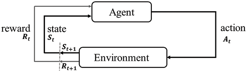
Figure 1: Reinforcement learning framework

Reinforcement learning is especially well suited to solve problem which involves long-term vs. short-term payoff tradeoffs, and it is widely used in real-world applications such as robot control, elevator scheduling, backgammon, checkers, and Go Game.

Q-Learning is a value-based reinforcement learning algorithm based on the Time Difference (TD) control algorithm of off-policy, Q that is Q (s, a), which involves the following equation:

Q(s,a)←Q(s,a)+α(Rsa+γmaxa′Q(s′,a′)−Q(s,a))(1)

2.2 LSTM

Long short-term memory (LSTM) [22] is widely used in artificial intelligence and deep learning for tasks such as unsegmented, connected handwriting recognition, speech recognition, and so on. This is due to the fact that it can process not only individual data points (e.g., images) but also entire data sequences (e.g., speech or video).

The structure of RNN was first proposed in 1990, which introduces the concept of recursive layers to choose whether to retain previous information or not, but RNNs do not maintain long-term dependence well due to gradient disappearance and gradient explosion problems. To address these issues, Kharitonov [23] proposed the long short-term memory network (LSTM), which introduces a gate structure to solve the gradient disappearance and gradient explosion problems during long sequence training. In summary, this means that LSTM can outperform standard RNN in longer sequences.

The LSTM can remember important information for a long time while forgetting unimportant information, and it can control the transmission state by gating the state. LSTM is well suited for processing and predicting time series problems due to its structure.

The common LSTM cell is made up of a cell, an input gate, an output gate, and a forgetting gate that remembers the values over any time interval, and three gates that control the flow of information to and from the cell.

The cell state is always present in the whole chain system of LSTM, ft is the forgetting gate, σ denotes the sigmoid function whose output is between 0 and 1, and tanh is the hyperbolic tangent function whose output is between −1 and 1. C is the control parameter that determines what information will be retained and what information will be forgotten. The weight of the control forgetting gate is denoted by wf.

The equation used are as follows:

Ct=ft∗Ct−1+it∗C~t(2)

The role of the forgetting gate is to decide which information in the previous moment is discarded from the cell state, i.e., a vector is calculated based on the current input xt and the previous moment output  ht−1. If the result is 0, it means that the LSTM should delete the corresponding information, and if it is 1, it is retained.

ft=σ(Wf⋅[ht−1,xt]+bf)(3)

The role of the input gate is to decide which information is stored in the cell state. The input gate will decide which information is added to Ct−1 to generate the new state Ct based on xt and  ht−1, and then the old state and the new state will be superimposed to get the new state.

it=σ(Wi⋅[ht−1,xt]+bi)(4)

Ct~=tanh⁡(WC⋅[ht−1,xt]+bC)(5)

2.3 Federated Learning

Federated learning [21] is a novel distributed learning algorithm that Google introduced in 2016. The federated learning framework is divided into two major parts. The first is the central server, where all participants collaborate train a federation model, i.e., a global model, with the support of the central server.

The federated learning model outperforms the models trained using only the participants’ own data. The second component is the data owner, which is comprised of the participants. It typically consists of N participants {L1,L2,L3,…,LN}, with each participant using their own local data {D1,D2,D3,…,DN}, to train the local model. It is then uploaded to the central server, and because each participant’s original data does not leave the local area, it is not exposed to other participants or third parties. To ensure privacy, Google’s proposed federated learning uses a combination of secure convergence and differential privacy. In other studies, homomorphic cryptographic protection parameters were used to achieve privacy protection.

The FL framework’s general training flow is as follows: The client (local user) device downloads the send model from the central server and trains it with local data. Following the completion of local training, each client uploads its updated model to the central server for model aggregation, which results in a shared global model. That after that, it is distributed to each client, so that each client and the central server continue to communicate with each other, and after a certain number of times, a global model with strong generalization ability can be obtained.

3  Methodology

In this paper, we propose the FedRL method for predicting household energy consumption, which is based on Federated Learning and Reinforcement Learning. Each household’s local data is trained using LSTM networks, households encrypt and upload the parameters of their local models to the central server. In the process, the households only share the parameters of their local models and not the actual data. The central server collects the local models uploaded by each household and uses the Q-learning algorithm to assign weights to the local models uploaded by each local. The Q values converge through successive training iterations, at which point the optimal model in this round of communication is obtained, and the optimal model is then sent to each household in each round, while the local model continues to be trained with updates.

3.1 Overall Framework

In this subsection, we present the framework of our proposed FedRL method for a clearer understanding of our energy consumption prediction process as shown in Fig. 2.

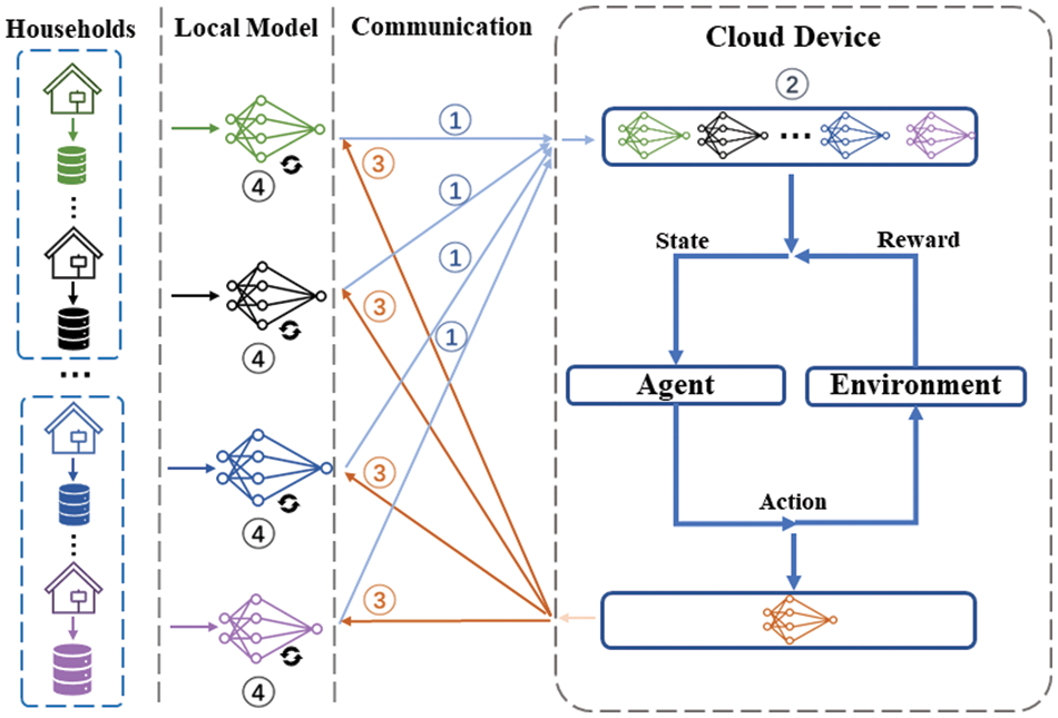
Figure 2: The overall framework of FedRL model

There are four layers in Fig. 2, the household layer, the local model layer, the communication layer, the central server layer. Each household has its own local private data, which is not shared with the central server or other households during the training process. In the local model layer, each household has its own local model, which we train by LSTM network using local data and encrypted upload to the central server after the training is completed; in the communication layer, the household and the central server share information. The decentralized models and the function of model aggregation are held by the central server layer, which also maintains the global models. In the cloud server layer, we perform model fusion and assign weights to the models uploaded by each household. The output in this round of communication is an ideal global model. The goal of federating optimization at the central server is to obtain an optimal global model with great generalization capacity.

Each step is described in greater detail below:

①   Local models are trained in households using local energy consumption data, and the gradient information is encrypted using encryption algorithms before being uploaded to the central server.

②   The central server collects local models from each household, uses reinforcement learning to assign weights to the uploaded local models, and then distributes the optimal global model to each household after obtaining the optimal global model for each round.

③   The central server obtains the best global model for each round of communication and distributes it to each household.

④   Households receive the most current global model and use local data to update the local model.

3.2 MDP Modeling

We model the energy consumption prediction process as an MDP and define the state, action and reward functions. In the model training process, we obtain the optimal model in this round of communication by successive training iterations where the Q values converge. Then we send the optimal model to each household, and each household continues training, thus keeping iterating to the specified number of communication rounds to obtain the optimal global model. The specific modeling components are as follows:

1)     Constructing the state space. We set the weight occupied by the local model to the state S={S1,S2,S3,…,St}. It is the value of the weight occupied by each local model as {m1,m2,m3,…,mn}, which sum up to 1.

2)     Constructing the action space

The weight change value of the weight occupied by the local model to the action space A={A1,A2,A3,…,At}. The sum of the action change values is 0.

3)     Constructing the reward function

W is the model after fusion of weights for each round in Q-learning. W is updated iteratively on the validation set, resulting in a new MSE for each round. We set the reward to the difference of MSE. If the MSE difference between the next state and this state is greater than zero, we will award a negative one reward. Otherwise, the reward is a plus one. The reward function is as follows:

R={−1 MSEt−MSEt−1>0  0  MSEt−MSEt−1=0 1 MSEt−MSEt−1 < 0 (6)

3.3 Algorithm Design

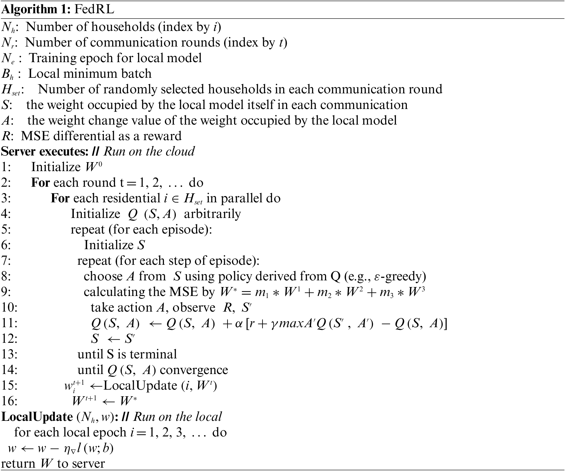
We present the algorithm design of the FedRL method. We use the Q-learning algorithm to assign weights to each locally uploaded local model. And keep iterating to the specified number of communication rounds to obtain the optimal global model.

Set the local epoch Ne=1, the local batch size Blocal=20, and the number of interactions (communication rounds) between the local and central server Nr=10. We select 10% of the households in each round of communication to participate in model training.

Algorithm 1 describes in detail the training process of the proposed model:

4  Experiments and Results

We conduct a large number of experiments to validate the proposed model’s prediction performance. Section 3.1 will provide a brief overview of the experimental setting and datasets used. Our prediction accuracy evaluation metrics are presented in Section 3.2. Section 3.3 compares and contrasts our model to centralized and distributed models.

4.1 Experimental Setting

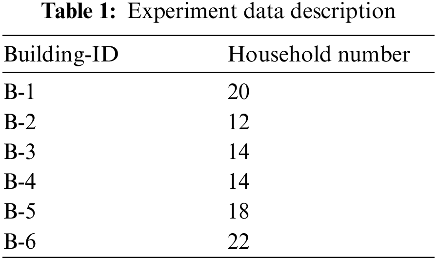
We select to use a dataset collected in London by the energy provider UK Power Networks and made public. The dataset contains data gathered by 5567 smart meters between November 2012 and February 2014, with smart meters taking readings every half hour, i.e., data at a granularity of 30 min, expressed in kwh (kilowatts per half hour). We assume that the number of households in a building is assigned at random to different households based on the building. We can predict the total electricity consumption of the building, which may assist the grid company in properly allocating electricity to the community. We eventually decide to study the data collected from January 01, 2013 to December 31, 2013, selecting 100 households in Building-1 to Building-6, and the number of households selected for each building is shown in the Table 1 below:

We partition the dataset into training, validation and test sets at the ratio of 7:1:2. Households are trained locally with LSTM networks using their respective local data, and the optimizer in the network used for training was stochastic gradient descent (SGD), with the learning rate set to 0.01 and the dropout set to 0.2. Set the local epoch Ne=1, the local batch size Blocal=20, and the number of interactions (communication rounds) between the local and central server Nr=10. We select 10% of the households in each round of communication to participate in model training.

In the FedRL model, the local data of the households are only trained locally and do not go out locally, because federated learning can share knowledge without violating the privacy of the households. In previous studies, Kharitonov [23] proposed using-local differential privacy to protect client data and protect the client from violations. In addition to protecting client privacy through differential privacy methods, homomorphic encryption algorithms can be used in federated learning. Kharitonov [23] used a homomorphic encryption algorithm to encrypt data during client-side local model training in order to protect user privacy. As a result, households only upload encrypted local model parameters and do not share their personal information.

Following the collection of each household’s local models by the central server, we use the Q-learning algorithm to assign weights to the individual locally uploaded local models when the central server performs model fusion. We set the weight occupied by the local model itself in each communication to the state S and set the weight change value of the weight occupied by the local model to the action space A, W is updated iteratively on the validation set, and a new MSE is generated in each round, and the difference in MSE is used as the reward. The best model is then assigned to each household, which uses local data for local model updates. Besides, we performed a simple data processing of the raw data, removing the abnormal data and replacing it with data collected the previous moment and data collected the next moment by adding and averaging the data.

4.2 Evaluation Measurements

In order to verify the predictive performance of the proposed method, three common evaluation metrics are used in this study, namely Mean Absolute Error (MAE), Mean Square Error (MSE), and Root Mean Square Error (RMSE). n denotes the number of samples, yi denotes the true value of the i th sample, and  y^i denotes the predicted value of the i th sample. MAE has better robustness to outliers, while MSE is simpler to compute. MAE is a common loss function used in regression models, and is the sum of the absolute values of the differences between the target and predicted values, and takes values from 0 to positive infinity. Calculation using Eq. (8). MSE is the sum of squares of the distance between the predicted and true values and is calculated as Eq. (9):

MAE=1n∑i=1n|yi−y^i|(7)

MSE=1n∑i=1n(yi−y^i)2(8)

RMSE=1n∑i=1n(yi−y^i)2(9)

4.3 Analysis of Experimental Results

4.3.1 Comparison with Centralized Methods

There are numerous methods for predicting energy consumption, the majority of which use centralized models, so we compare four methods: DT, RF, BPNN, and LSTM. First, we experimented with the model’s predicted trends, using building-1 as an example in the FedRL model, and the experimental results are shown in Fig. 3.

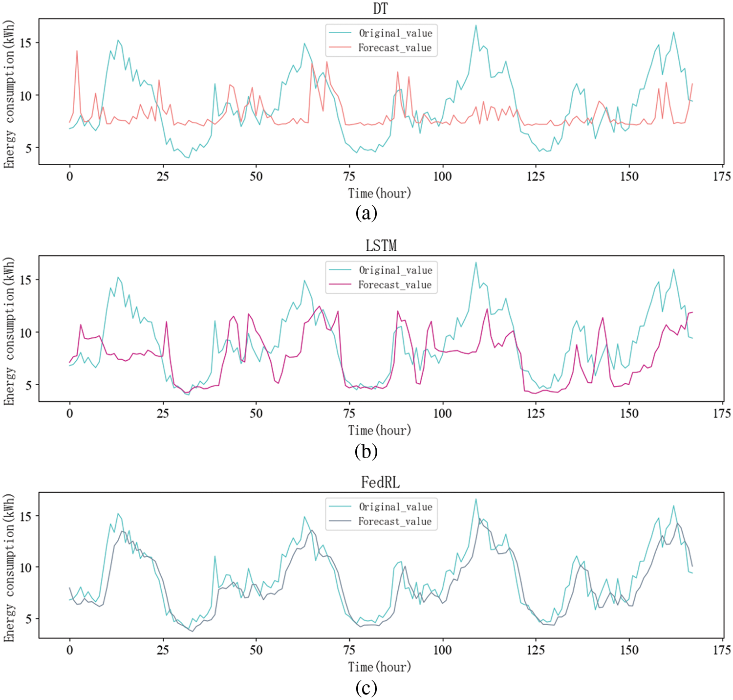
Figure 3: Forecasting trends for different centralized methods

In Fig. 3, the horizontal axis represents the predicted time Hours, and the vertical axis represents the residential energy consumption value. We select a forecast period of 7 days. That is to say, 168 h. In Fig. 3a, the DT method is difficult to predict continuous values, and sometimes it is easy to overfit, so it can only predict the general trend, and the prediction of some peaks is still lacking. In Fig. 3b, because of the use of neural networks, LSTM can already predict the general prediction trend better than traditional machine learning, but prediction accuracy still needs to be improved.

In Fig. 3c, it can be seen that compared to other models, the FedRL method predicts the overall trend and the peak to be very close to the true value. This is due to the fact that individual households are trained using local data. In comparison to centralized model training, The FedRL model trains the model using local data in each household, then uploads the encrypted local model to the central server, and each household collaborates to train the model for energy prediction. In comparison to the centralized model, the FedRL model protects occupant privacy and prevents home privacy leakage.

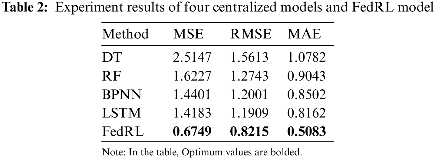
To further validate the accuracy of our prediction performance, we show the experimental results of the four Centralized models DT, RF, BPNN, LSTM, and FedRL model in Table 2. FedRL has MSE = 0.6749, RMSE = 0.8215, and MAE = 0.5083, as shown in the Table 2. Simultaneously, the FedRL method’s RMSE improved by 36.9% when compared to the centralized model’s prediction performance.

4.3.2 Comparison with Distributed Methods

In this subsection, we compare the FedRL model with other distributed models, the other models are FedSGD, FedAvg, FedAtt, all four methods are distributed prediction methods, all with building-1 in the experiment, and the prediction trends of the four methods are shown in Fig. 4.

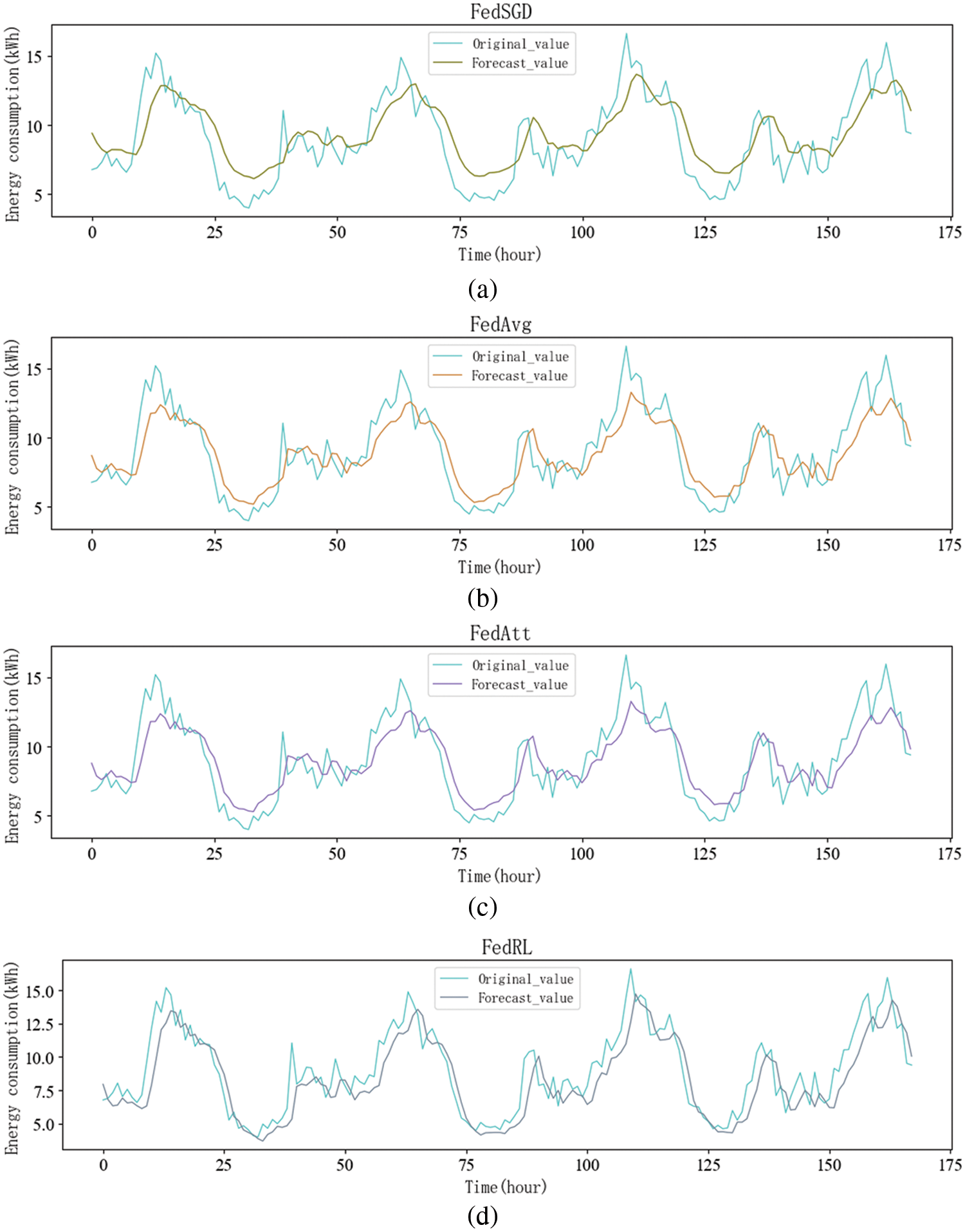
Figure 4: Prediction trends of different distributed models

In Fig. 4, the horizontal axis represents the predicted time Hours, and the vertical axis represents the residential energy consumption value. We select a forecast period of 7 days. That is to say, 168 h. Figs. 4a and 4b show that the prediction trends for both the FedSGD and FedAvg methods are roughly the same. This is because FedAvg is an improvement on FedSGD, and the main improvement advantage is that by dividing batches locally and reducing communication time between the local and the central server, there is no obvious advantage in terms of prediction accuracy. In Figs. 4b and 4c, there is not much of a difference between the FedAtt and FedAvg methods. Fig. 4d shows the trend prediction graph of the FedRL model, which is more accurate in predicting the trend compared to the other three models.

However, based solely on the prediction trend of each method in the graph, the advantage of our model is not immediately apparent, so we present the experimental results of the four methods in the Table 3.

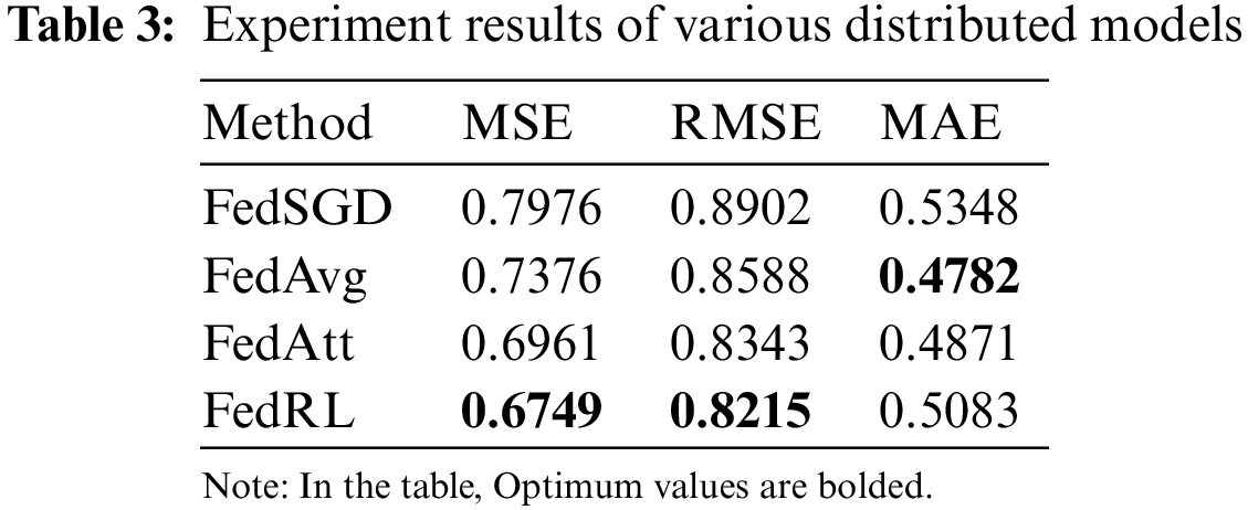
As shown in Table 3, our model’s prediction accuracy outperforms the other three models, with 3.7% higher than RMSE and 3.2% higher than MSE. In comparison to the traditional FedAvg, we have integrated reinforcement learning into the cloud. Compared to weighted averaging directly in the cloud, using the Q-learning algorithm to assign weights to each locally uploaded local model, we obtain the optimal model in this round of communication, and then we newly send it to each household, and each household continues to train, and thus we keep iterating to the specified number of rounds of communication to obtain the optimal global model. The final experimental results show that the prediction accuracy of FedRL model outperforms the other models.

5  Conclusions and Discussion

Most studies have experimented with predicting energy consumption by pooling data for model training. However, the process of centralizing data can result in data leakage. If a household’s private information leaks, it might easily put people’s lives and possessions in grave danger. Moreover, many laws and regulations have been enacted regarding data security and privacy, making it difficult to centralize data. This can lead to the problem of data silos, where data is not allowed to be shared between different users. The FedAvg method is used in all classical federated learning frameworks for security aggregation to directly weigh average the model parameters, which may have an adverse effect on model performance.

In order to solve the above problems, the FedRL method is proposed in this study as an energy consumption prediction method based on federated learning and reinforcement learning. The method improves on FedAvg by incorporating the Q-learning algorithm. We add a Q-learning algorithm to assign weights to each uploaded local model. When the central server performs secure aggregation, it assigns weights to each locally uploaded local model. In each communication, we set the weight occupied by the local model to the state S and the weight change value of the weight occupied by the local model to the action space A. W is updated iteratively on the validation set, resulting in a new MSE for each round. The reward is the difference in MSE. If the MSE difference between the next state and this state is greater than zero, we will award a negative one reward. Otherwise, the reward is a plus one. The Q value converges through successive training iterations. We get the optimal model in this round of communication is obtained. Then we send the optimal model to each household, and each household continues training, thus keeping iterating to the specified number of communication rounds to obtain the optimal global model.

We evaluated our proposed method using a dataset of energy consumption in London and obtained experimental results of 0.6749 for MSE, 0.5083 for MAE and 0.8215 for RMSE. In the beginning, it is compared to four centralized models: DT, RF, BPNN, and LSTM. In the FedRL model, each household collaboratively trains the global model, local data does not leave the local area, and only the encrypted gradient parameters are uploaded in such a way that energy prediction can be performed, preventing the leakage of household privacy. Meanwhile, the FedRL method’s RMSE improved by 36.9% when compared to the centralized model’s prediction accuracy. The FedSGD, FedAvg, and FedAtt distributed models are then compared. Our model’s prediction accuracy is superior to the classical FedAvg, with 3.7% higher than RMSE and 3.2% higher than MSE.

We discovered a problem during the experiment, the communication time between each family and the central server is long, which means that the communication consumption between each client and the server is large. The number of participating households in the experiment is not large at the moment, and we can afford the cost of this communication, but if we have thousands of households involved in training, or even more, I think this is something that can be explored in depth in future work on the efficiency of communication.

Funding Statement: This work was financially supported by National Key R&D Program of China (No. 2020YFC2006602), National Natural Science Foundation of China (Nos. 62172324, 62072324, 61876217, 6187612), University Natural Science Foundation of Jiangsu Province (No. 21KJA520005), Primary Research and Development Plan of Jiangsu Province (No. BE2020026), Natural Science Foundation of Jiangsu Province (No. BK20190942).

Conflicts of Interest: The authors declare that they have no conflicts of interest to report regarding the present study.

References

1. Himeur, Y., Ghanem, K., Alsalemi, A., Bensaali, F., Amira, A. (2021). Artificial intelligence based anomaly detection of energy consumption in buildings: A review, current trends and new perspectives. Applied Energy, 287, 116601. https://doi.org/10.1016/j.apenergy.2021.116601 [Google Scholar] [CrossRef]

2. Kang, H., An, J., Kim, H., Ji, C., Hong, T. et al. (2021). Changes in energy consumption according to building use type under COVID-19 pandemic in South Korea. Renewable and Sustainable Energy Reviews, 148, 111294. https://doi.org/10.1016/j.rser.2021.111294 [Google Scholar] [PubMed] [CrossRef]

3. Paramati, S. R., Shahzad, U., Doğan, B. (2022). The role of environmental technology for energy demand and energy efficiency: Evidence from OECD countries. Renewable and Sustainable Energy Reviews, 153, 111735. https://doi.org/10.1016/j.rser.2021.111735 [Google Scholar] [CrossRef]

4. Zhang, M. (2022). A preliminary study on China’s territorial spatial planning under the double carbon goal. 2nd International Conference on Materials Chemistry and Environmental Engineering (CONF-MCEE 2022), pp. 176–181. Zhuhai, China. [Google Scholar]

5. Zou, B., Ju, C., Bao, F., Lai, Y., Xu, C. et al. (2022). Exploring an efficient evolutionary game model for the government–enterprise–public during the double carbon policy in China. International Journal of Environmental Research and Public Health, 19(8), 4607. https://doi.org/10.3390/ijerph19084607 [Google Scholar] [PubMed] [CrossRef]

6. Ahmadiahangar, R., Häring, T., Rosin, A., Korõtko, T., Martins, J. (2019). Residential load forecasting for flexibility prediction using machine learning-based regression model. 2019 IEEE International Conference on Environment and Electrical Engineering and 2019 IEEE Industrial and Commercial Power Systems Europe (EEEIC/ICPS Europe), pp. 1–4. USA. [Google Scholar]

7. Wang, S., Xu, X. (2006). Simplified building model for transient thermal performance estimation using GA-based parameter identification. International Journal of Thermal Sciences, 45(4), 419–432. https://doi.org/10.1016/j.ijthermalsci.2005.06.009 [Google Scholar] [CrossRef]

8. Ma, Y., Yu, J. Q., Yang, C. Y., Wang, L. (2010). Study on power energy consumption model for large-scale public building. 2010 2nd International Workshop on Intelligent Systems and Applications, pp. 1–4. IEEE. [Google Scholar]

9. Hong, Y., Zhou, Y., Li, Q., Xu, W., Zheng, X. (2020). A deep learning method for short-term residential load forecasting in smart grid. IEEE Access, 8, 55785–55797. https://doi.org/10.1109/Access.6287639 [Google Scholar] [CrossRef]

10. Guo, Q., Feng, Y., Sun, X., Zhang, L. (2017). Power demand forecasting and application based on SVR. Procedia Computer Science, 122, 269–275. https://doi.org/10.1016/j.procs.2017.11.369 [Google Scholar] [CrossRef]

11. Ekonomou, L. (2010). Greek long-term energy consumption prediction using artificial neural networks. Energy, 35(2), 512–517. https://doi.org/10.1016/j.energy.2009.10.018 [Google Scholar] [CrossRef]

12. Hou, Z., Lian, Z. (2009). An application of support vector machines in cooling load prediction. 2009 International Workshop on Intelligent Systems and Applications, pp. 1–4. IEEE. [Google Scholar]

13. Yaslan, Y., Bican, B. (2017). Empirical mode decomposition based denoising method with support vector regression for time series prediction: A case study for electricity load forecasting. Measurement, 103, 52–61. https://doi.org/10.1016/j.measurement.2017.02.007 [Google Scholar] [CrossRef]

14. Sajjad, M., Khan, Z. A., Ullah, A., Hussain, T., Ullah, W. et al. (2020). A novel CNN-GRU-based hybrid approach for short-term residential load forecasting. IEEE Access, 8, 143759–143768. https://doi.org/10.1109/Access.6287639 [Google Scholar] [CrossRef]

15. Agatonovic-Kustrin, S., Beresford, R. (2000). Basic concepts of artificial neural network (ANN) modeling and its application in pharmaceutical research. Journal of Pharmaceutical and Biomedical Analysis, 22(5), 717–727. https://doi.org/10.1016/S0731-7085(99)00272-1 [Google Scholar] [PubMed] [CrossRef]

16. Li, Y. (2017). Deep reinforcement learning: An overview. arXiv preprint arXiv:1701.07274. [Google Scholar]

17. Somu, N., MR, G. R., Ramamritham, K. (2021). A deep learning framework for building energy consumption forecast. Renewable and Sustainable Energy Reviews, 137, 110591. https://doi.org/10.1016/j.rser.2020.110591 [Google Scholar] [CrossRef]

18. Brunke, L., Greeff, M., Hall, A. W., Yuan, Z., Zhou, S. et al. (2022). Safe learning in robotics: From learning-based control to safe reinforcement learning. Annual Review of Control, Robotics, and Autonomous Systems, 5, 411–444. https://doi.org/10.1146/annurev-control-042920-020211 [Google Scholar] [CrossRef]

19. Guo, X., Zhao, Q., Zheng, D., Ning, Y., Gao, Y. (2020). A short-term load forecasting model of multi-scale CNN-LSTM hybrid neural network considering the real-time electricity price. Energy Reports, 6, 1046–1053. https://doi.org/10.1016/j.egyr.2020.11.078 [Google Scholar] [CrossRef]

20. Ozcan, A., Catal, C., Kasif, A. (2021). Energy load forecasting using a dual-stage attention-based recurrent neural network. Sensors, 21(21), 7115. https://doi.org/10.3390/s21217115 [Google Scholar] [PubMed] [CrossRef]

21. Yang, Q., Liu, Y., Cheng, Y., Kang, Y., Chen, T. et al. (2019). Federated learning. Synthesis Lectures on Artificial Intelligence and Machine Learning, 13(3), 1–207. https://doi.org/10.1007/978-3-031-01585-4 [Google Scholar] [CrossRef]

22. Memarzadeh, G., Keynia, F. (2021). Short-term electricity load and price forecasting by a new optimal LSTM-NN based prediction algorithm. Electric Power Systems Research, 192, 106995. https://doi.org/10.1016/j.epsr.2020.106995 [Google Scholar] [CrossRef]

23. Kharitonov, E. (2019). Federated online learning to rank with evolution strategies. Proceedings of the Twelfth ACM International Conference on Web Search and Data Mining, pp. 249–257. Haikou, China. [Google Scholar]

24. Li, L., Fan, Y., Tse, M., Lin, K. Y. (2020). A review of applications in federated learning. Computers Industrial Engineering, 149, 106854. https://doi.org/10.1016/j.cie.2020.106854 [Google Scholar] [CrossRef]

25. Bonawitz, K., Eichner, H., Grieskamp, W., Huba, D., Ingerman, A. et al. (2019). Towards federated learning at scale: System design. In: Proceedings of machine learning and systems, vol. 1, pp. 374–388. [Google Scholar]

26. Li, T., Sahu, A. K., Talwalkar, A., Smith, V. (2020). Federated learning: Challenges, methods, and future directions. IEEE Signal Processing Magazine, 37(3), 50–60. https://doi.org/10.1109/MSP.79 [Google Scholar] [CrossRef]

27. Banabilah, S., Aloqaily, M., Alsayed, E., Malik, N., Jararweh, Y. (2022). Federated learning review: Fundamentals, enabling technologies, and future applications. Information Processing Management, 59(6), 103061. https://doi.org/10.1016/j.ipm.2022.103061 [Google Scholar] [CrossRef]

28. Thapa, C., Arachchige, P. C. M., Camtepe, S., Sun, L. (2022). Splitfed: When federated learning meets split learning. Proceedings of the AAAI Conference on Artificial Intelligence, pp. 8485–8493. Vancouver, Canada. [Google Scholar]

29. Manoharan, P., Walia, R., Iwendi, C., Ahanger, T. A., Suganthi, S. T. et al. (2022). SVM-based generative adverserial networks for federated learning and edge computing attack model and outpoising. Expert Systems, e13072. https://doi.org/10.1111/exsy.13072. [Google Scholar] [CrossRef]

30. Pei, J., Zhong, K., Jan, M. A., Li, J. (2022). Personalized federated learning framework for network traffic anomaly detection. Computer Networks, 209, 108906. https://doi.org/10.1016/j.comnet.2022.108906 [Google Scholar] [CrossRef]

31. Tan, A. Z., Yu, H., Cui, L., Yang, Q. (2022). Towards personalized federated learning. IEEE Transactions on Neural Networks and Learning Systems, pp. 1–17. IEEE. https://doi.org/10.1109/TNNLS.2022.3160699. [Google Scholar] [PubMed] [CrossRef]