Modelling Dry Port Systems in the Framework of Inland Waterway Container Terminals

1  Introduction

Making logistics systems sustainable requires pivoting away from traditional approaches used to plan such systems-that is, not developing modes of transport separately [1]. Achieving sustainability is indeed possible with intensive planning and the development of intermodal transport (IT) systems [2]. Per the European Conference of Ministers of Transport [3], IT refers to the movement of goods in a particular loading unit or vehicle via two or more modes of transport without handling the goods when shifting between modes. With the application of alternative modes of transport-rail, inland waterway, and sea transport-a logistics system can save on costs and become more time-efficient while reducing negative impacts on the environment [4]. Although the apparent advantages of applying IT have motivated numerous researchers in the field to promote its use [5], IT remains neglected in practice. Aside from the multiple attempts of the European Union to promote the application of IT in different projects, its participation in overall transport remains less than satisfactory [6,7].

One of the missing links in European IT systems is the stimulation of the utilisation of inland waterways in IT chains. Achieving economies of scale in inland waterway transport is entirely possible and can not only result in cost-competitiveness when putting against road transportation [8] but also external costs that are lower than those of other modes of transport [9,10]. Although the advantages of inland waterway transport are evident, its application, aside from in north-western Europe [11], has been stagnant for decades [10,12], with inadequate connections with rail transport highlighted as the chief obstacle to integrating inland waterway transport in existing IT systems [13]. The consequences of that shortcoming are relatively narrow catchment areas for river container terminals that fail to direct larger container flow volumes to inland waterway transport.

One of the most explored categories of IT terminals in the context of developing IT systems is the dry port (DP). A DP is a subsystem of a seaport in the seaport’s hinterland that encompasses an established regular rail shuttle and road connection with the seaport and offers services at the seaport’s container terminals [14]. Using DPs can boost the competitiveness of seaport container terminals and their catchment areas, which consequently attracts larger container flow volumes [15,16] and facilitates integration with the IT system in the hinterland [15]. DPs are pivotal components for expanding the geographic impact of seaports and, in turn, intensifying the economic development of the regions where they are located [17]. То achieve all of those benefits, however, DP-based IT systems require appropriate network modelling, which is often a complex task. Aside from developing IT systems by applying the concept of DPs for seaport container terminals, Tadić et al. [2] have highlighted an opportunity for developing DP systems in the framework of inland waterway container terminals (IWCTs).

The purpose of this article is to investigate the concept of DPs in the framework of IWCTs. The main hypothesis is that developing DP terminals for existing IWCTs can expand their catchment areas and, by establishing regular shuttle connections between DP terminals and IWCTs, enable the efficient integration of inland waterway transport into existing IT systems. The article’s principal contribution is in being the first to address the modelling of DP systems in the framework of IWCTs. The modelling of such DP system should answer the questions that refer to the number and location of DP terminals for IWCTs, their capacity, and their allocation of container flows. The second hypothesis states that it is possible to develop an encompassing and robust approach for modelling such DP concept that will adequately treat the complex nature of the problem through the lens of sustainability. In this study, we solved those problems by using a mathematical formulation that considers several different objective functions, along with a novel hybrid metaheuristic model that we developed specifically to solve the problems. The model is based on the Bee Colony Optimisation (BCO) algorithm and the measurement of alternatives and ranking according to the compromise solution (MARCOS) multi-criteria decision-making (MCDM) method. Another contribution is that we applied the model to assess the Danube region, an area that has been poorly covered in similar research. The results of this study indicate that the development of the DP concept in the framework of IWCTs could stand out as a potentially sustainable direction for developing regional IT networks. The sensitivity analysis implies that the concept is sustainable for different settings of evaluation criteria thus confirming its great potential.

In what follows, Section 2 presents a brief review of the literature on the concept of DPs, with an emphasis on research addressing the modelling of DP systems and on the methods used for problem-solving within that domain. Next, Section 3 describes the mathematical formulation for the observed problem of modelling DP systems in the framework of IWCTs, after which Section 4 explains our procedure for the combined application of BCO and MARCOS, the model set-up for solving the observed problem, and the steps of solution evaluation and modification by the model. Last, Section 5 discusses the input parameters and values of the hybrid metaheuristic model, the results of its application and conducts a sensitivity analysis, followed by Section 6, which offers our conclusions and recommends directions for future research.

2  Frame of Reference

Flows of goods have intensified due to globalisation and changes in the principles of production, particularly individualisation and personalisation. As a result, the trend of delivering small quantities of goods over greater distances has arisen and thereby increased the geographic areas for goods and transport flows [18]. To accommodate those trends, ports have been forced to develop IT networks in their hinterlands with the aim of increasing the geographic scope of door-to-door services through collaborative agreements and vertical integration [12]. Because ports thus increasingly lack space for expansion and become denser over time, a solution should be sought in developing ports’ hinterlands by applying the concept of DPs [12,19].

A popular topic in the scientific community [20], the concept of DPs has been a subject of analysis in the context of regional and intercontinental sea container terminals around the world. Such research has covered areas on all populated continents: Europe [21–23], Asia [16,24,25], North America [26], South America [27], Africa [28] and Australia [29,30]. A large portion of such research has focused on modelling DP systems, and a brief literature review of recent research in the field, with highlighted characteristics and applied models, is presented in Table 1. In the context of that literature, this article is unique because it focuses on modelling DP systems in the framework of IWCTs.

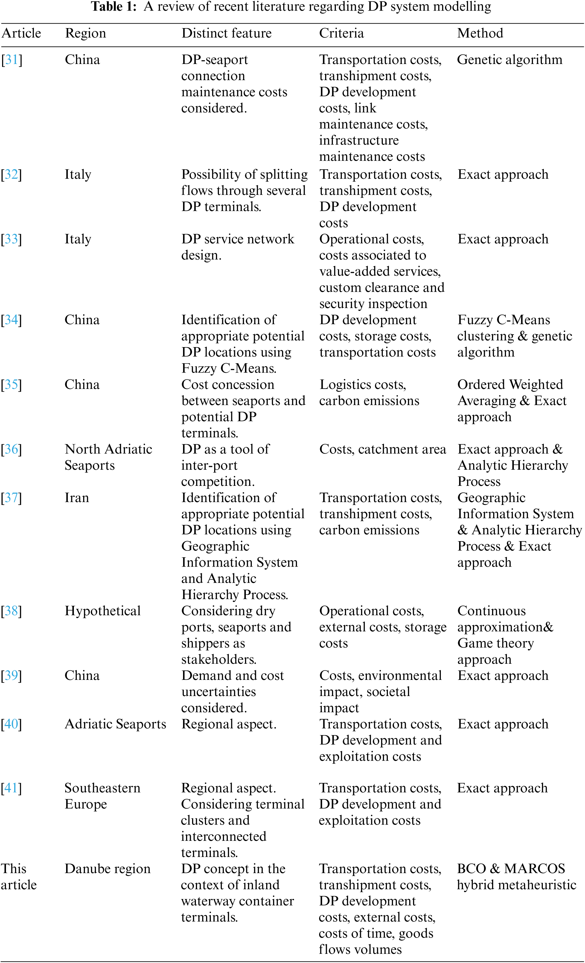
Table 1 clarifies that though solutions to the problem of modelling DP systems have been diverse, the research driving those solutions has shared certain characteristics. All such research has considered some kind of cost structure while modelling DP systems, mostly operational costs and the costs of developing DP terminals. Some of it has also considered external costs (e.g., [35,37–39]). The research that tackled the DP system modelling problems in a multi-objective way failed to include a broader set of objective functions that would reflect on all three sustainability pillars (economic, environmental and social) and the complex nature of such problems. Within that literature, Kramberger et al. [36] have analysed how the degree to which DP terminals in the north Adriatic are developed affects their catchment areas and competitiveness in comparison with northern European seaport container terminals. Aside from that study, most of the research has analysed the concept of DPs in the context of a single state or country, whereas studies investigating the concept of DPs in regional contexts have been few [36,40,41]. However, developing DP systems, as well as IT systems in general, should be done in broader regional contexts, even if such a venture requires international collaboration when individual actors (e.g., countries) are incapable of developing comprehensive IT systems by themselves. This article contributes to the existing literature by approaching the modelling of a DP system through a regional perspective. While doing so, this article encompasses multiple objective functions that reflect on all three sustainability pillars and demonstrates how the complex nature of the problem should be treated.

The diversity of problems involved in implementing not only DPs but also IT in general justifies the application of different methods for solving them. The most-used methods and approaches for solving such problems are simulation models [25,42], MCDM methods [17,43], exact approaches [32,33,41], and metaheuristic algorithms [31,34,44]. Of all of those strategies, metaheuristic algorithms have proven to be efficient for solving complex combinatorial problems regarding some aspects of IT. Several popular metaheuristics in that literature have been used in IT, including genetic algorithms [31], memetic algorithms [45], simulated annealing [46,47], tabu searches [48], adaptive large neighbourhood searches [49], particle swarm optimisation [50], and greedy randomised adaptive searches [51,52]. Against that background, this article presents the first application of the BCO metaheuristic for solving an IT-related problem. This is another significant contribution of this article because it demonstrates a robust and encompassing approach to solving complex multi-objective optimization problems.

The BCO metaheuristic, inspired by the natural behaviour of bees, has proven to be a competitive metaheuristic for solving combinatorial optimisation problems, namely by providing high-quality solutions for complex problems in acceptable computational time frames [53,54]. Different classes of problems have been solved with BCO, including the p-centre problem [55], the anti-covering location problem [56], vehicle routing [57], transit network planning [58], airport gate assignment [59], berth allocation [60], traffic control [61], detector placement on transport networks [62], tuning of fuzzy membership functions [63], etc. To treat the complex nature of the problem appropriately, the MARCOS MCDM method is integrated into the BCO.

The MARCOS MCDM method defines the relationship of alternatives- in our case, feasible solutions- according to the ideal and anti-ideal solution [64], and that relationship is the basis for determining the degree of the utilization, or quality, of alternatives or solutions [65]. By combining the concepts of ratio and reference point sorting, the MARCOS method has proven to be stable and insensitive to the change in measurement scales [65]. A comparison with other MCDM methods, including TOPSIS, EDAS, MABAC, SAW, ARAS, and WASPAS, has revealed that the MARCOS method is relatively efficient, comprehensive and stable [65]. Aside from its independent application, the method has also been combined with other MCDM methods, including SWARA [66], FUCOM [64], Delphi and FARE [2], but never with a metaheuristic algorithm for solving multi-criteria optimization problems. The competitiveness of the MARCOS method in the domain of MCDM and its potential for uncomplicated combination with other methods were our chief reasons for integrating it with a metaheuristic algorithm in our study.

3  Mathematical Formulation of the Problem

This section describes the mathematical formulation of the problem of modelling DP systems in the framework of IWCTs. The problem entails determining the number and location of DP terminals, their capacity, and their allocation of container flows. The formulation was inspired by pre-existing formulations for modelling DP systems [32,35,41] but adapted to the problem of developing DP systems for IWCTs by considering several objective functions in order to treat the problem in the most realistic way possible.

To be clear, this article examines the possibility of developing DP terminals in the framework of IWCTs and establishing a combined road–rail–inland waterway transport for observed container flows to achieve sustainability in the IT system. The network that we observed in our study consists of flow generators and IWCTs, wherein the generators initiate the flows of goods and a certain exchange of different goods exists between them. Our initial assumption was that all of the flows are transported via road. The developed DP terminals play the role of local or regional consolidation centres and enable modal transformation from road to rail given the relationship between DPs and IWCT, after which inland waterway transport is used. Although the possibilities of combining different modes of transport are numerous, in this article the combinations are narrowed down to ones that are the most realistic and feasible to implement (Fig. 1).

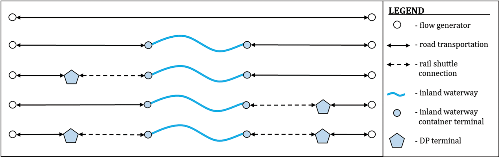
Figure 1: The considered container flow shipping variants

To adequately describe the observed problem, the following parameters are used:

•   F-set of all container flows that have to be shipped. Each container flow (f) is defined by:

● Its origin (fo),

● Destination (fd),

● Type of goods (fc),

● Volume of goods expressed in Twenty-foot Equivalent Units (TEUs) (qf),

● The average weight of one TEU for the type of goods (qfc).

D-the set of potential locations for developing DP terminals.

L-the set of IWCTs.

Considering fo and fd of a container flow f, along with IWCTs l1 and l2 as well as DP terminals d1 and d2, there are five different variants of container flow realization: directly by road transportation (fofd), through IWCTs l1 and l2 (fol1l2fd), through the DP terminal d1 and IWCTs l1 and l2 (fod1l1l2fd), through IWCTs l1 and l2 and the DP terminal d1 (fol1l2d1fd), or through DP terminals d1 and d2 and IWCTs l1 and l2 (fod1l1l2d2fd). Each of these variants has its assigned transportation unit costs, external unit costs, and time unit costs:

●   Cfofdtran, Cfol1l2fdtran, Cfod1l1l2fdtran, Cfol1l2d1fdtran, Cfod1l1l2d2fdtran-transportation unit costs of flow f for the observed realization variants.

●   Cfofdext, Cfol1l2fdext, Cfod1l1l2fdext, Cfol1l2d1fdext, and Cfod1l1l2d2fdext-external unit costs of flow f for the observed realization variants.

●   tfofd, tfol1l2fd, tfod1l1l2fd, tfol1l2d1fd, and tfod1l1l2d2fd-time unit costs for the types of goods in flow f for the observed realization variants.

G-the set of considered terminal size categories.

Cgtranshipment-the transhipment cost for one TEU in a terminal in category g.

Cgcategory-the development cost of a terminal in category g.

CgQ-the maximal throughput of allocated flows for such a terminal.

Cltranshipment-the transhipment cost of one TEU in IWCTl.

Cl−basictranshipment-the transhipment cost of one TEU in IWCTl if that IWCT does not have an assigned DP.

Decision variables used in the formulation are:

•   Xf (binary variable) equals 1 if the container flow f is shipped only by road; 0 if otherwise.

•   Xl1l2f (binary variable) equals 1 if the container flow f is being shipped via road–inland waterway transport through IWCTs l1 and l2; 0 if otherwise.

•   Xd1l1l2f (binary variable) equals 1 if the container flow f is shipped through DP terminal d1 and subsequently through IWCTs l1 and l2; 0 if otherwise.

•   Xl1l2d1f (binary variable) equals 1 if the container flow f is first shipped through IWCTs l1 and l2 and subsequently through DP terminal d1; 0 if otherwise.

•   Xd1l1l2d2f (binary variable) equals 1 if the container flow f is shipped through DP terminal d1, next through IWCTs l1 and l2, and later through DP terminal d2; 0 if otherwise.

•   Lld (integer variable) denotes how many DP terminals IWCT l has an established connection with.

•   Yd (binary variable) equals 1 if a DP terminal is located in d; 0 if otherwise.

•   Wdg (binary variable) equals 1 if DP terminal d is, by capacity, in category g; 0 if otherwise.

•   Qd (integer variable) refers to the number of TEUs that flow through DP terminal d.

•   Ql (integer variable) refers to the amount of containers in TEUs that pass through IWCT l.

With such parameters and definitions of variables, the problem can be mathematically formulated as follows:

min:∑fFqf⋅fc⋅(Xf⋅Cfofdtran+∑l1L∑l2LXl1l2f⋅Cfol1l2fdtran+∑d1D∑l1L∑l2L(Xd1l1l2f⋅Cfod1l1l2fdtran+Xl1l2d1f⋅Cfol1l2d1fdtran)+∑d1D∑d2D∑l1L∑l2LXd1l1l2d2f⋅Cfod1l1l2d2fdtran)+∑dD∑gGWdg⋅Qd⋅Cgtranshipment+∑lL⋅ Ql⋅Cltranshipment(1)

min:∑fFqf⋅fc⋅(Xf⋅Cfofdext+∑l1L∑l2LXl1l2f⋅Cfol1l2fdext+∑d1D∑l1L∑l2L(Xd1l1l2f⋅Cfod1l1l2fdext+Xl1l2d1f⋅Cfol1l2d1fdext)+∑d1D∑d2D∑l1L∑l2LXd1l1l2d2f⋅Cfod1l1l2d2fdext)(2)

min:∑fFqf⋅Cftime(Xf⋅tfofd+∑l1L∑l2LXl1l2f⋅tfol1l2fd+∑d1D∑l1L∑l2L(Xd1l1l2f⋅tfod1l1l2fd+Xl1l2d1f⋅tfol1l2d1fd)+∑d1D∑d2D∑l1L∑l2LXd1l1l2d2f⋅tfod1l1l2d2fd)(3)

min:∑dD∑gGWdg⋅Cgcategory(4)

max:∑fFqf⋅(∑d1D∑l1L∑l2L(Xd1l1l2f+Xl1l2d1f)+∑d1D∑d2D∑l1L∑l2LXd1l1l2d2f)(5)

with the following constraints:

Xf+∑l1L∑l2LXl1l2f+∑d1D∑l1L∑l2LXd1l1l2f+∑d2D∑l1L∑l2LXl1l2d2f+∑d1D∑d2D∑l1L∑l2LXd1l1l2d2f=1∀f∈F(6)

Yd≥Xdl1l2f+Xl1l2df+Xdl1l2d2f+Xd2l1l2df∀d,d2∈D;d≠d2;f∈F;l1,l2∈L;l1≠l2(7)

Lld≥Xdll2f+Xdl2lf+Xdll2d2f+Xdl2ld2f∀d,d2∈D;d≠d2;f∈F;l,l2∈L;l≠l2(8)

∑d∈DLld≤1;∀l∈L(9)

Qd≥∑fF(qf⋅(∑l1L∑l2L(Xdl1l2f+Xl1l2df)+∑d2D∑l1L∑l2L(Xdl1l2d2f+Xd2l1l2df)))∀d∈D(10)

Ql≥∑fF(qf⋅(∑l2L(Xll2f+Xll2f)+∑d1D∑l2L(Xd1ll2f+Xll2d1f)+∑d1D∑d2D∑l2L(Xd1ll2d2f+Xd2ll2d1f)))∀l∈L(11)

Qd≤∑gGWdg⋅CgQ∀d∈D(12)

∑g∈GWdg=1∀d∈D(13)

Cltranshipment≥Cl−basictranshipment+∑d1D∑gG(Wdg⋅Cgtranshipment⋅Lld1−Cl−basictranshipment)∀l∈L(14)

Objective Function 1 minimises the overall operational costs of the system, which consist of transportation costs, transhipment costs in DP terminals and transhipment costs in IWCTs. Objective Function 2 minimises the external costs of the system, while Objective Function 3 minimises the time costs (i.e., losses) of goods; the time costs of goods are treated as a separate objective function in order to highlight the different compatibilities of particular types of goods with inland waterway transport and IT in general. Next, Objective Function 4 minimises the development costs of DP terminals, while Objective Function 5 maximises the volume of container flows in the catchment area of the DP system. To reiterate, our goal was to develop a system with the largest possible catchment area, which is a prerequisite for achieving regional sustainability.

As for the constraints, Constraint 6 ensures that every flow can be shipped in only one way, while Constraint 7 keeps track of the locations where the DP terminals are developed. Constraint 8 keeps track of the DP terminal connections for the IWCTs, where the number of connections of one IWCT is limited to 1 by virtue of Constraint 9. Constraint 10 keeps track of the container flows that pass through DP terminals, while Constraint 11 keeps track of the same parameter for IWCTs. Constraint 12 ensures that the volumes of container flows that pass through DP terminals do not exceed their capacities. The capacity constraints for IWCTs were intentionally excluded because our goal was to develop a new system able to attract more intermodal flows, which is not constrained by the existing capacity limitations of IWCTs. The existing capacities are mostly small and, even as such, mostly unutilized, which confirms that the current system is inadequately used. Constraint 13 ensures that the DP terminals as located have only one assigned category of terminal capacity. Last, Constraint 14 for transhipment costs in the IWCTs establishes the transhipment costs of its assigned DP terminal. In the case that an IWCT lacks an assigned DP terminal, the basic transhipment cost (Cl−basictransshipment) is assigned.

4  A Hybrid BCO-MARCOS Metaheuristic Model

For this article, we developed a novel hybrid BCO–MARCOS metaheuristic model to solve the mathematical problem described in Section 3–the problem of modelling DP systems for IWCTs, for the case of the Danube region. To address the combinatorial complexity of the problem, a metaheuristic approach was selected, while the presence of several objective functions justified the integration of a MCDM method into the process of evaluating solutions. The role of the BCO algorithm was to search the solution space for feasible solutions, while the MARCOS method was used in their evaluation. The generalized algorithmic steps of the developed BCO–MARCOS model are presented in Fig. A1 (Appendix), while the following subsections provide detailed explanations of the BCO metaheuristic and MARCOS MCDM method.

4.1 The BCO Metaheuristic

The initial variant of the BCO algorithm defined a constructive approach to problem-solving [53], but a later variant based on solution improvement was developed [54] and is used in this article as well. The algorithmic steps of the BCO metaheuristic based on solution improvement are as follows [53,54]:

Input parameters-number of bees (m), number of forward passes (i.e., flights) per iteration (Nf), and termination criteria-are initialized, and the initial solution is defined.

In every iteration, every bee executes Nf forward passes. At the beginning of every iteration, the best-known solution (BKS) is assigned to all bees. During each forward pass, a bee modifies its solution based on the defined modification operators, and every solution modification is followed by a backward pass.

During a backward pass, every bee evaluates the quality of its solution in relation to the solutions of other bees. For maximization problems, the ith bee’s normalized solution value (Oi) is determined by the following equation:

Oi=Φi−ΦminΦmax−Φmin(15)

in which Φi is the aggregated value of the quality of the solution of the ith bee according to all objective functions, and Φmax and Φmin respectively represent the best- and worst-aggregated values of the quality of the solution for all bees in the observed flight. From another angle, Φi is in fact the output value of the MARCOS–MCDM method, whose algorithmic steps are explained in the next subsection.

Based on the quality of the solution, for every bee i the probability that it remains loyal to its solution (piloyal) is determined by using the following equation:

piloyal=e−Omax−Oin(16)

in which Omax represents the largest normalized value of the solutions’ quality for all bees in the observed flight n. For every bee i, a random number within the interval between 0 and 1 is generated, and if the number is less than the value of piloyal, then the bee remains loyal to its solution.

After returning to the hive, bees that remained loyal to their solutions recruit non-loyal bees. The probability that the loyal bee k is followed (pkfollowing) is determined according to the following equation:

pkfollowing=Ok∑q∈LkOq(17)

in which Ok represents the normalized value of the quality of the solution for bee k, and Lk represents the set of all loyal bees.

Based on the roulette wheel method, every non-loyal bee determines which loyal bee to follow in the next forward pass.

The iterations are repeated until the criterion for termination is met. In the case that a better solution than the BKS is found at any moment, the BKS is updated.

4.2 The MARCOS MCDM Method

The input parameters for the MARCOS method are the set of alternatives (R)-in our case, the set of bees’ solutions in the observed flight-along with the set of criteria (C)-in our case, the objective functions described in Section 3-weight coefficients of the objective functions (wj), and the decision matrix Δ. The decision matrix Δ is composed of the bees’ solution values for all objective functions in the observed flight, in which xij represents the ith bee’s solution value according to the objective function j for the observed flight, m is the number of bees, and n is the number of objective functions. In the framework of our hybrid metaheuristic model, the MARCOS method is executed in the third step of the BCO metaheuristic (i.e., Eq. (15)). To analyse whether the solutions of bees are better than the current BKS, the current BKS is also considered in their evaluation.

The algorithmic steps of the MARCOS method were adapted from [64] for the context of its integration with the BCO method:

To evaluate the solutions of bees in the observed flight, the BKS is included in the decision matrix, which can be expanded by defining the ideal (Rid) and anti-ideal (Rai) solution:

Δ=RaiR1R2⋮RmBKSRid C1C2⋯Cn[ xai1xai2x11x12x21x22⋯xain⋯x1n⋯x2n⋮⋮xm1xm2xBKS1xBKS2xid1xid2⋮⋮⋯xmn⋯xBKSn⋯xidn ](18)

Thus, Cmax is the set of all maximization objective functions, and Cmin is the set of all minimization objective functions. Rid and Rai are defined according to the following equations:

Rai=min1≤i≤m+1xij,  j∈Cmax  and  max1≤i≤m+1xij,  j∈Cmin(19)

Rid=max1≤i≤m+1xij,  j∈Cmax  and  min1≤i≤m+1xij,  j∈Cmin(20)

The normalised decision matrix U=[uij]m+1×n is formed according to the following equation:

uij=xidxij,  j∈Cmin(21)

uij=xijxid,  j∈Cmax(22)

The weighted matrix V=[vij]m+1×n is formed by multiplying the elements of matrix U with the corresponding objective function weight coefficients according to the following equation:

vij=uij⋅wj(23)

The degree of the utility of bee’s solutions Ki is calculated in relation to Sai and Sid:

Ki−=SiSai(24)

Ki+=SiSid(25)

in which Si represents the sum of all elements of the weighted matrix V for the ith bee’s solution:

Si=∑j=1nvij(26)

while Sai and Sid represent the Si parameter value for Rai and Rid solution.

The value of the utility function Φi is determined for every bee’s solution in the observed flight by using the following equation:

Φi=Ki++Ki−1+1−f(Ki+)f(Ki+)+1−f(Ki−)f(Ki−)(27)

in which f(Ki+) represents the utility function in relation to Rid, and f(Ki−) represents the utility function in relation to Rai, both of which are determined according to the following equations:

f(Ki+)=Ki−Ki++Ki−(28)

f(Ki−)=Ki+Ki++Ki−(29)

The solutions of the bees are ranked according to the parameter Φi. Solutions with a greater value of Φi are considered to be better. If a solution exists that, according to the parameter Φi is better than the current BKS, then that solution is updated to be the new BKS. The values Φi represent the basis upon which the quality of the bee’s solution is determined in the third step of the BCO.

4.3 Solution Evaluation and Modification by the Bees

The most time-consuming part of solving IT network modelling problems is evaluating the objective function of the solutions because it requires allocating observed flows within the given network structure. Allocating flows in IT networks is a problem in itself that various studies have examined (e.g., [67,68]). In our work, allocating flows is only one component of a more complex problem that entails determining the number of DP terminals and their location, connecting the terminals with appropriate IWCTs, and determining their capacity. In our model, after a solution is modified by a bee, it is necessary to again allocate the container flows for the new system structure in order to evaluate the solution according to all of the objective functions. Thus, the allocation of container flows is executed every time that a solution is modified by a bee and according to the same rules for all bees.

Flows for a given IT network structure can be allocated by applying a heuristic approach inspired by Sörensen et al. [51]. The idea of the heuristic is to determine the priority of allocation based on the costs and benefits of the allocation. Its application thus allows prioritizing the allocation of flows that contribute to improving the observed objective functions. The priority of allocating the observed container flow f (f∈F) to the DP terminal d (Priorityfd), in which d∈D, is determined according to the following equation:

Priorityfd=Qf⋅wop⋅Sopf,d+we⋅Sef,d−wt⋅Stf,dmax{wop,we,wt}(30)

in which Qf represents the intensity of the flow f in TEUs, while Sopf,d, Sef,d, and Stf,d respectively refer to the operational savings, external costs savings, and time costs when flow f passes through the terminal d. Beyond that, wop,we, and wt are the weighted coefficients of those objective functions, respectively.

For every evaluated IT network structure, we formed a list consisting of the Priorityfd values for all flows and all possible flow shipping variants. The list is sorted in descending order, and the flows are allocated according to the sorted list and their Priorityfd value while considering the existing capacities of DP terminals as located. That approach affords the advantage of allocating flows that most contribute to improving the objective functions.

We defined three types of bees that differ in how they modify the solution. For each type of bee, a certain level of uncertainty (i.e., randomized search) exists during the modification of a solution in order to ensure diversity when exploring the space of feasible solutions.

Type 1 bees modify a solution by opening new DP terminals or closing an existing DP terminal. The decision to open a new DP terminal d (d∈D) for a randomly selected IWCT l (l∈L) is based on the parameter PotentialdL, which represents the maximum possible benefits of opening the terminal according to the sum of the elements Priorityfd in relation to d – l:

Potentialdl=∑f=1FPriorityfd−l(31)

When opening a DP terminal for IWCT l, the bee considers z closest locations for the observed IWCT (z∈D). The probability that a DP terminal is located at location d is calculated according to the following equation:

pdlocating=Potentialdl∑q=1zPotentialql(32)

According to probabilities pdlocating, the new location of a DP terminal is determined by the roulette wheel method, while terminal capacity is determined by choosing a random capacity category.

In the case of closing a DP terminal, the selection of the terminal is determined according to the capacity utilization of the existing DP terminals. The probability that the DP terminal d (d∈{∀d∈D|Yd=1}) is selected to be closed is determined according to the following equation:

pdclosing=(1−QdQdmax)∑q=1nd(1−QqQqmax)(33)

in which Qd represents the volume of container flows that pass through terminal d, Qdmax the capacity of terminal d, and nd the number of DP terminals as located. In that approach, priority for closing is given to DP terminals with less capacity utilization. Following the roulette wheel method according to probabilities pdclosing, a DP terminal to be closed is chosen. In the case that all terminals fully utilize their capacities, the DP terminal to be closed is selected at random. Because opening new and closing existing DP terminals are acts performed with one type of bee, it is predetermined in the model that in 70% of cases the bee will decide to open a new DP terminal.

Type 2 bees, by contrast, modify the solution by changing the category of terminal capacity for an existing DP terminal. Such bees choose one of the located terminals at random and, based on its TEU throughput, determine the two neighbouring (i.e., larger and smaller) categories of capacity. Next, the category of capacity is randomly selected between the two neighbouring categories.

Last, Type 3 bees modify the solution by changing the location of existing DP terminals. The probability that terminal d (d∈{∀d∈D|Yd=1}) is relocated is determined according to the following equation:

pdrelocating=1−Potentialdld∑q=1ntPotentialqlq(34)

in which ld represents the IWCT to which the DP terminal d is assigned. After choosing the terminal to relocate by using the roulette wheel method, z nearest locations to the DP terminals are determined, and a new location is subsequently chosen according to the probabilities from Eq. (32), also by using the roulette wheel method.

In a series of experiments, we determined that the best solutions could be obtained with the configuration of five bees: one type 1 bee, one type 2 bee and three types 3 bees. The number of forward passes per iteration was set to be 5. The criterion for terminating the model was 10 successive iterations without any improvement in BKS greater than 0.005 according to the parameter Φi. The experiment was conducted on a personal computer with an Intel Core i7-8750H central processing unit with 2.20 GHz and 8 GM of RAM memory.

5  Application of the Model for Solving the Observed Problem

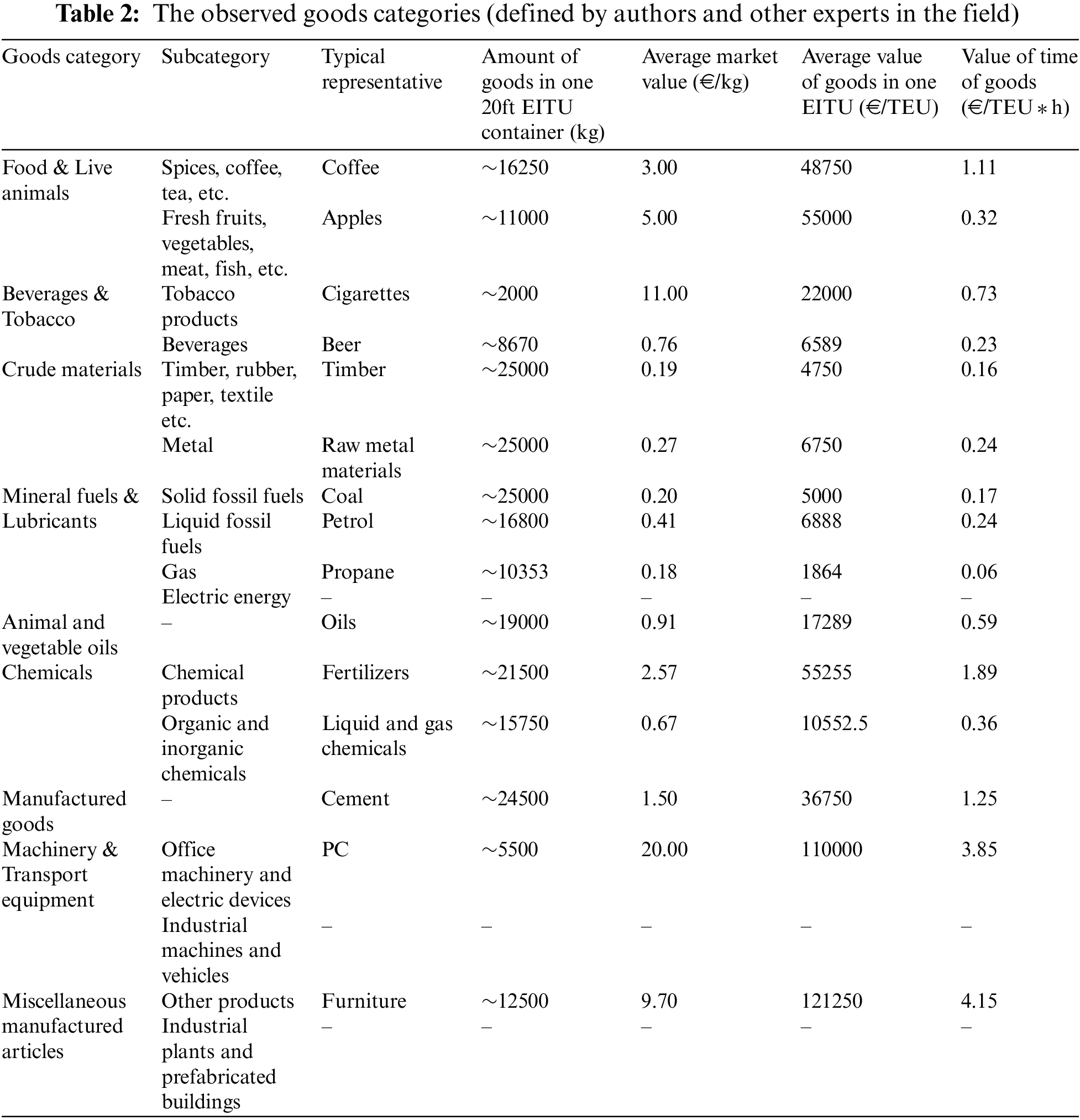
In our model, flow generators are represented as regional nodes, defined according to the official Nomenclature Of Territorial Units and Statistics at the second level (i.e., NUTS 2) and the region’s spatial-geographic characteristics. In our analysis, the primary categories of goods according to the Standard International Trade Classification [69] were taken into account. Every category of goods was divided into logical subcategories, for each of which a typical representative, its characteristics, the average amount of goods per container, and average market value were determined (Table 2). The value of time for different goods was determined with reference to [70], which, though dated, is the only work known to us that considers the matter in an appropriate way.

According to the official statistics of Eurostat and the national governments of countries in the Danube region, the volume of goods traded between pairs of countries is determined for all subcategories of goods. The quantity of goods between generator pairs is proportionally distributed according to the population of the regions where those generators are located. Our analysis included generators from 14 countries or regions: southern Germany, Austria, Czech Republic, Slovakia, Hungary, Romania, Moldova, Ukraine, Slovenia, Croatia, Bosnia and Herzegovina, Serbia, Montenegro, and Bulgaria. Eight potential IWCTs in strategically important locations were also considered: Deggendorf, Linz, Vienna, Budapest, Baja, Belgrade, Ruse, and Giurgiulesti.

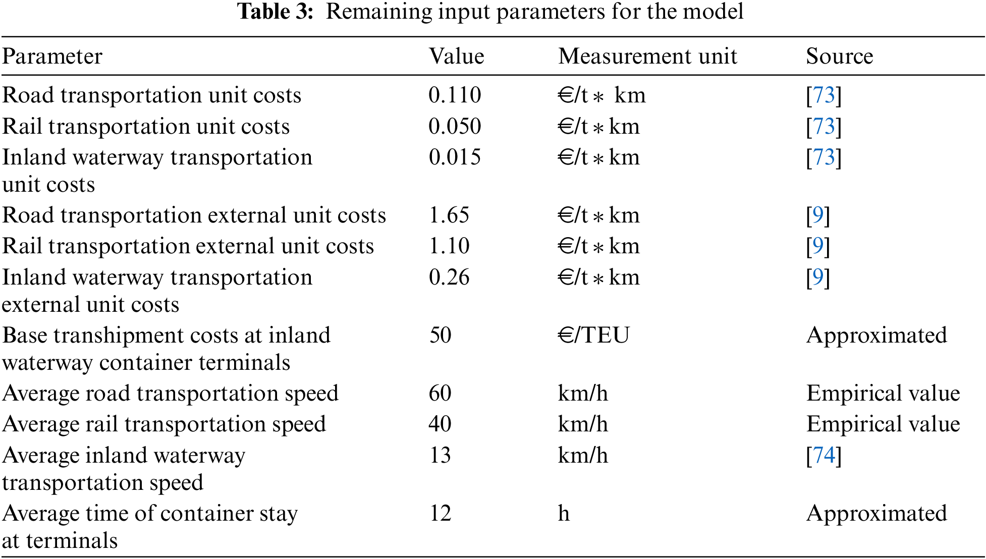
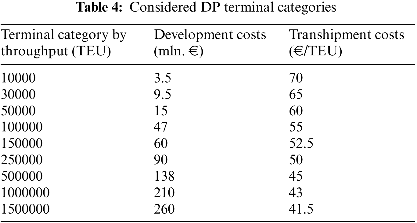
Other input parameters, presented in Table 3, were the per-unit transport and emission costs of different modes of transport, their average speed, basic transhipment costs in IWCTs, and the average length of container stays at the terminals. According to [2,17,71], our own experience in the field, and the characteristics of the problem, the weighted coefficients for the objective functions were 0.25 for operational costs, 0.22 for external costs, 0.16 for time costs, 0.13 for terminal development costs, and 0.24 for the amount of container flows attracted. Following Wiegmans et al. [72], nine different capacity categories of DP terminals were considered (Table 4). Terminals with greater capacity generally had greater development costs but lower transhipment costs per unit.

5.1 Results

Using the input parameters from Section 5.1 and Tables 2–4, the optimization problem, defined by Objective Functions 1–5 and Constraints 6–14, was solved. The BCO metaheuristic was applied according to the steps described in Section 4.1, Eqs. (15)–(17), and the solution modification described in Section 4.3 and Eqs. (30)–(34). During every evaluation of solutions following the third step of executing BCO, the MARCOS method was applied according to Eqs. (18)–(29). The observed optimization problem was solved in 15 executed instances in order to determine the stability of the developed BCO–MARCOS model. For the initial solution in every execution, a solution was generated with one DP terminal located according to the modification of type 1 bees for a randomly selected IWCT. The objective functions values for best-found solutions for every model execution are presented in Table 5.

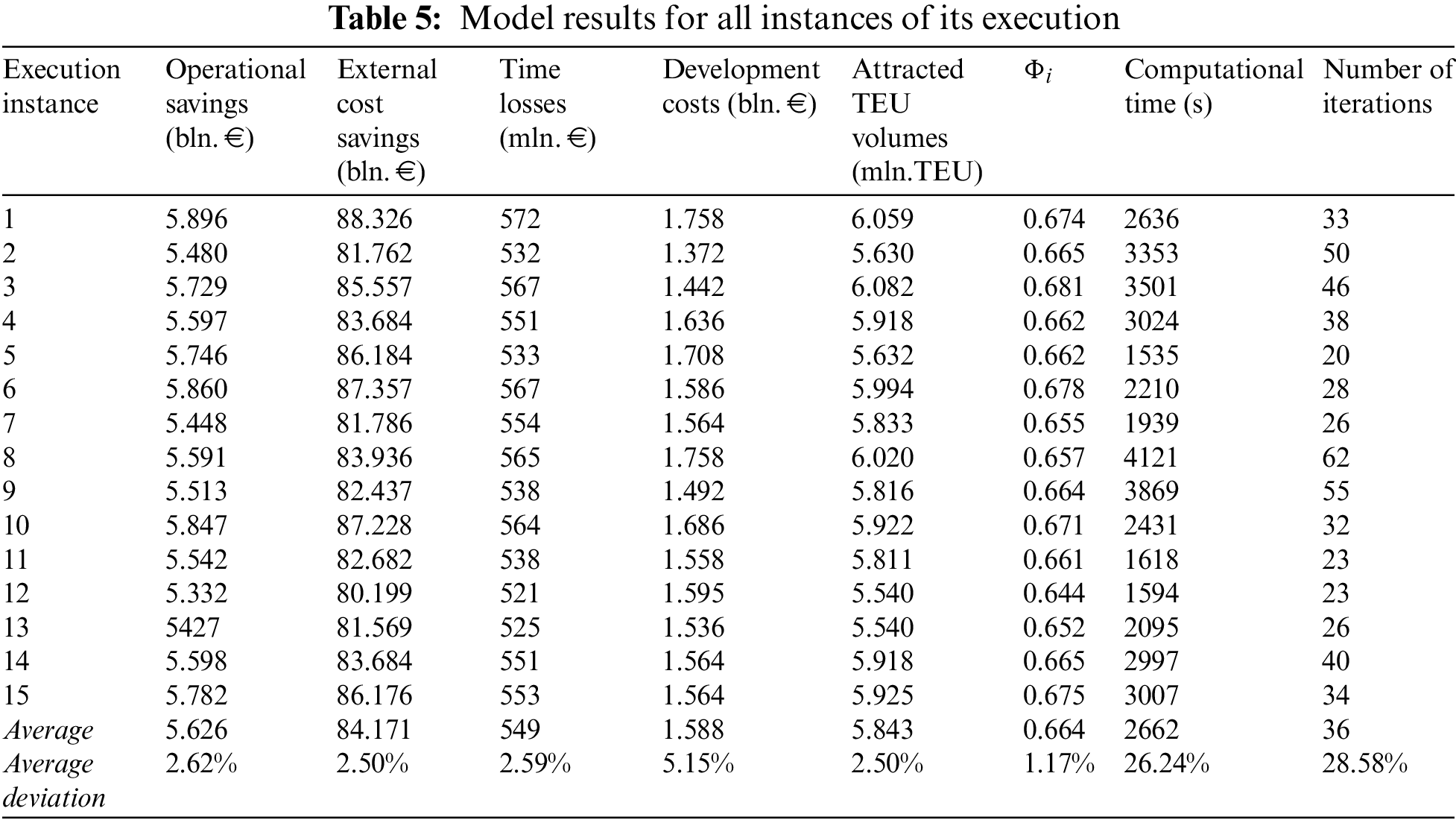
In all instances of the model’s execution, the result consisted of eight DP terminals. However, in some cases, variations existed in terminal location and terminal capacity as a consequence of the simultaneous optimisation of five objective functions. According to the results presented in Table 5, the average deviation of solution values for each of the five objective functions was small (2.62%, 2.50%, 2.59%, 5.15%, and 2.50%, respectively), which indicates that the model had good convergence, as confirmed by the average deviation of the parameter Φi of only 1.17% when comparing the best-found solution in all instances. The average computational time of the model was 2662 s, and the average number of iterations was 36, both of which can be considered to be low given the extreme complexity and size of the problem.

The best-found solution (i.e., Execution 3) involves developing one DP terminal for every analyzed IWCT (Fig. 2). Three of the DP terminals (i.e., at Munich for the IWCT in Deggendorf, at Graz for the IWCT in Vienna, and at Miskolc for the IWCT in Budapest) have a capacity of at least 1 million (e.g., 1.5 million TEUs for the Miskolc DP terminal), the DP terminal for the IWCT in Linz (Ceske Budejovice) has a throughput of 625,000 TEU, while the remaining terminals (i.e., Szeged for the IWCT in Baja, Kragujevac for the IWCT in Belgrade, Bucharest for the IWCT in Ruse, and Comrat for the IWCT in Giurgiulesti) have a capacity of 500,000 TEUs.

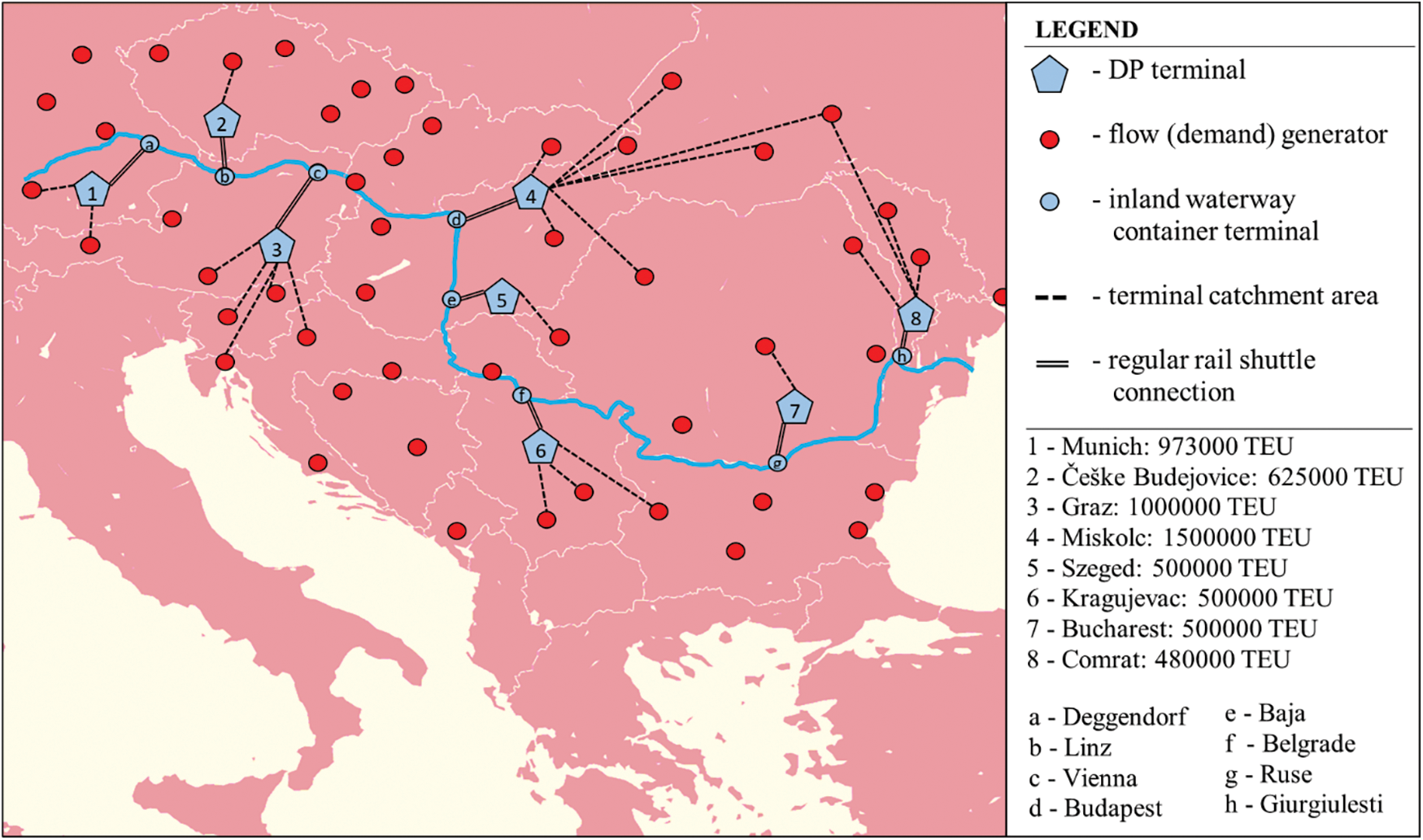
Figure 2: Output results–the best-found solution

The results are especially interesting considering that a relatively narrow region was analyzed. According to the model, developing eight DP terminals is justified. Such a result justifies implementing the concept of DPs for IWCTs, and it can be expected that with the analysis of a broader geographical area that the justification only becomes greater. To better examine the behaviour of the DP concept in the framework of IWCTs, a sensitivity analysis is conducted and presented in the next subsection.

5.2 Sensitivity Analysis & Discussion

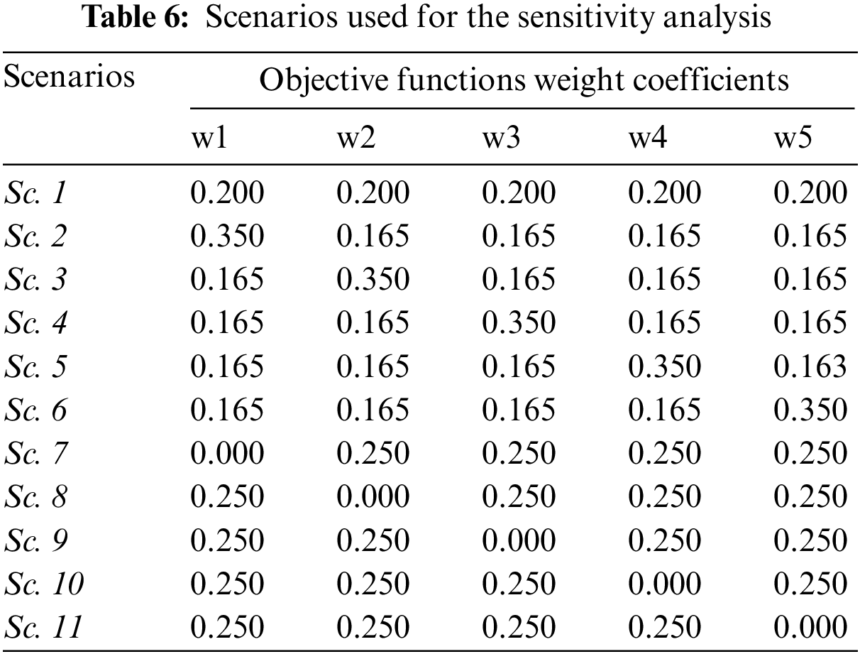
Output results of every multi-objective optimization problem are influenced. By the way, the objective functions’ importance is perceived and treated. To better understand the nature of the problem/solution, it is necessary to perform appropriate sensitivity analyses. To inspect the behaviour of the DP concept in the framework of IWCTs, the sensitivity analysis is conducted through 11 different scenarios. Scenarios differ in the configuration of weight coefficients for the objective functions (Table 6). In the first scenario (Sc. 1), all objective functions are treated equally (their weight coefficients are set to 0.2). In scenarios Sc. 2–Sc. 6, for every individual objective function, 0.350 is adopted as its weight coefficient while other weight coefficients were set to 0.165. This was done to see how the dominance of one objective function over others influences the final solution. In the remaining scenarios (Sc. 7–Sc. 11), one of the objective functions is excluded (its weight coefficient is set to 0), while the other objective functions were treated equally important (with weight coefficients set to 0.250).

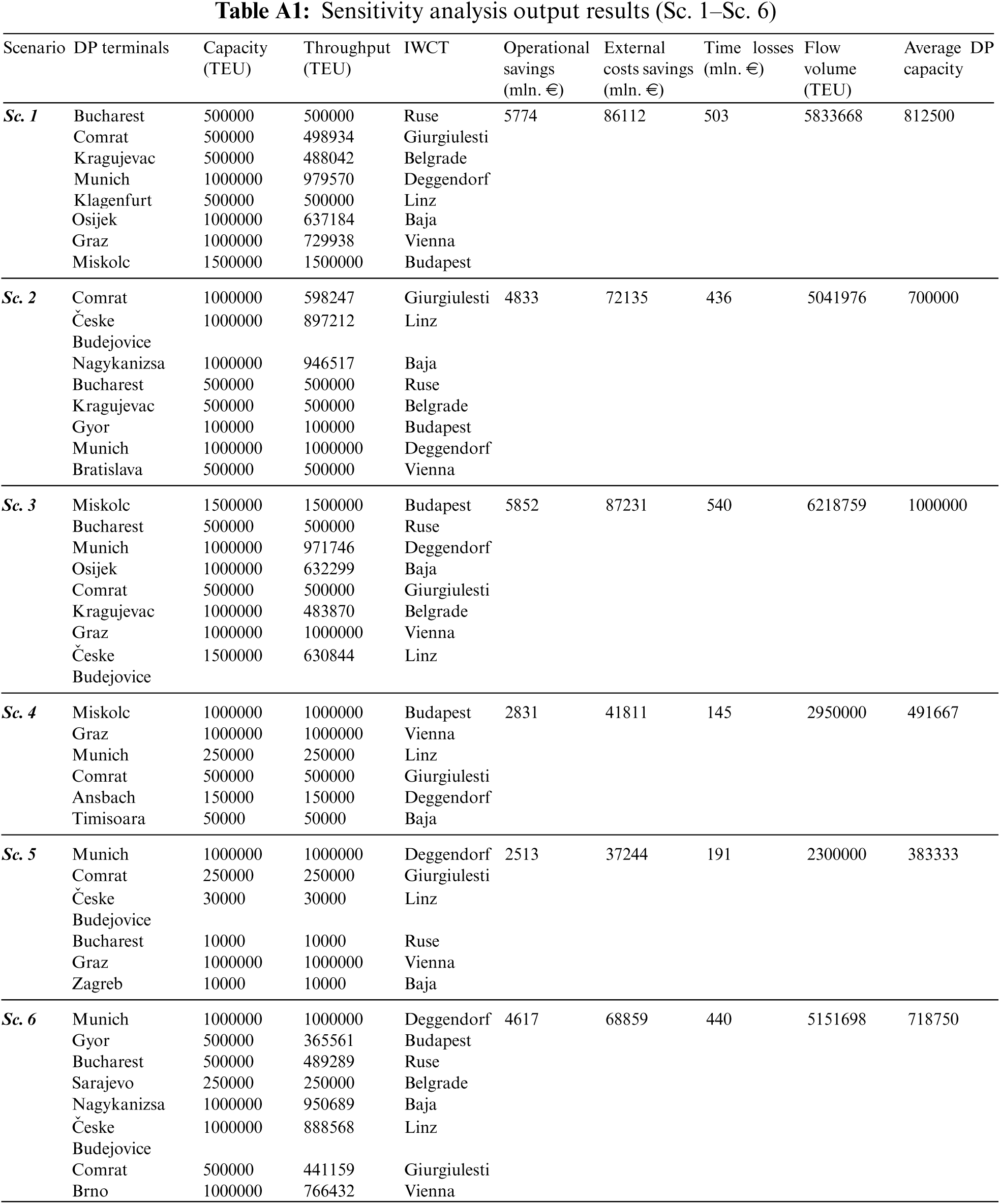
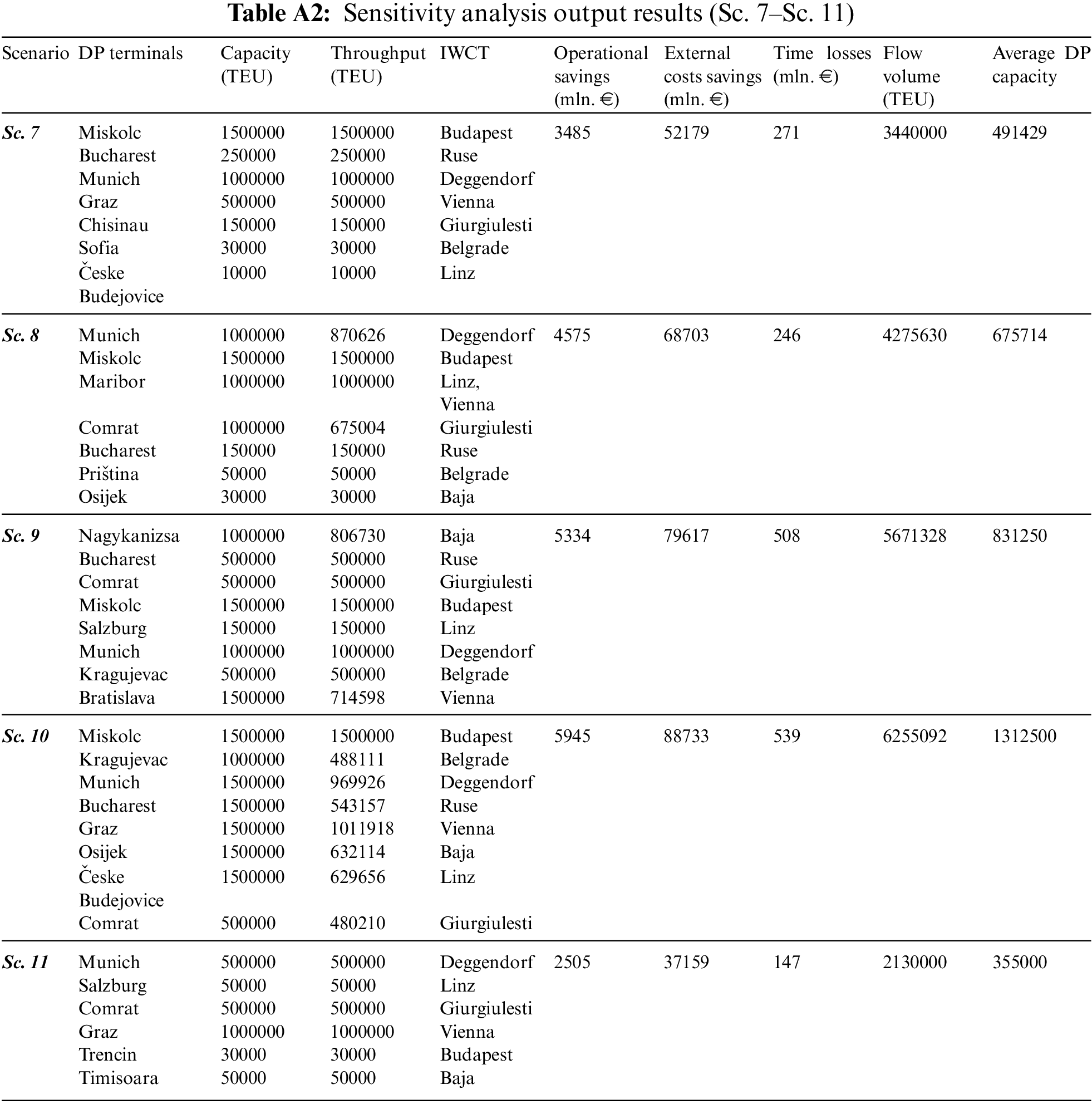
The application of the developed model over the defined scenarios showed that different solutions are obtained in different weight coefficient settings (Table 7). In scenarios Sc. 1, Sc. 2, Sc. 3, Sc. 6, Sc. 9, and Sc. 10, the results still imply that the development of DPs for every IWCT is justified. In scenarios Sc. 7 and Sc. 8, seven DPs emerged in the final solution. In the remaining scenarios (Sc. 4, Sc. 5 and Sc. 11), according to the results, the development of six DPs is justified. Depending on the scenario, the locations and capacities of DP terminals differ as well (Tables A1 and A2 in the Appendix).

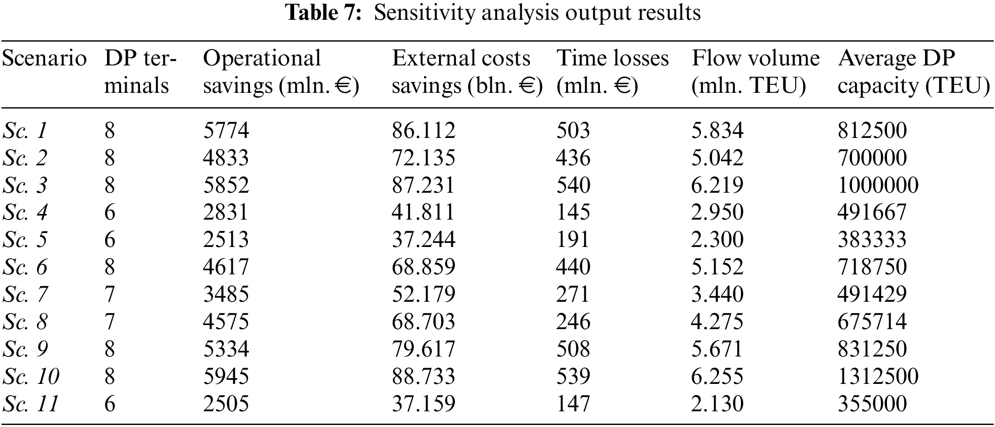
The sensitivity analysis indicates that the development of DP terminals in the framework of IWCTs is justified, but its configuration depends on the initial settings (objective function prioritization). This is natural since different objective functions tend to shape the solution in specific ways–some contribute to a specific concept while others are against it. Of course, the analysis in this article is limited to the five defined objective functions. More research should be done in different settings and configurations in order to better understand the advantages and weaknesses of the DP concept in the framework of IWCTs.

The purpose of this article has been to draw attention to the implementation of the concept of DPs for IWCTs, which can enable the efficient integration of inland waterway transport into IT systems. Developing such ports can significantly affect sustainability by reducing operational and external logistics costs. Although the results show that DPs in the framework of IWCTs can be sustainable, it is necessary to conduct more in-depth analyses of the possibilities and effects of their implementation.

The main limitation of this work is in considering a narrow geographical area around the Danube river. The article has proven that this is sufficient to illustrate the idea behind the concept and to demonstrate its potential sustainability. Another limitation is in not considering the stochastic nature of container flow characteristics. This would be a good direction for future research that will continue the examination of such DP concept variant. The container flows are narrowed down to the main goods categories, but further research could focus on some specific goods types and do more detailed analyses.

Several managerial insights could be drawn from the results. Firstly, policy creators in the field of IT are presented with another potentially sustainable development direction of IT systems–DP in the framework of IWCT. The developed model can help decision-makers to select locations for DP terminals and to narrow down future analyses to specific case studies of individual DPs. Stakeholders in the field of IT could conclude what specific locations/regions are potent for developing DP that will serve IWCTs in their region. The developed model, although developed for this specific problem, is universal in its nature and could be used, with minor tweaks and reconfigurations, to solve any multi-objective optimization problem in the domain of IT and other fields.

6  Conclusion

This article has examined the concept of DPs in the framework of IWCTs. Its chief contribution and the basis of its novelty is that it addresses modelling DP systems in the context of IWCTs. The article enriches an already versatile literature body regarding different configurations of DP-based IT systems but stands out as the only one that provides integration of inland waterways into existing IT systems. The article also contributes by treating the modelling of DP systems by virtue of the comprehensiveness of the problem’s formulation. The problem was mathematically formulated considering several objective functions. The selected objective functions are inherited from the existing literature and included simultaneously during the modelling of the observed DP concept, which has not been done in any previous research. Ultimately, its other contributions are the development of a novel hybrid BCO–MARCOS metaheuristic model for solving the problem and the demonstration of its application in the Danube region.

The results of the model’s application indicate the sustainability of the concept of DPs in the framework of IWCTs, even for narrow areas around inland waterways. According to the results, developing eight DP terminals in different categories in and for the Danube region is justified.

In the future, researchers should consider conducting more detailed analyses of the concept in a stochastic–dynamic environment, developing adequate evaluation models, and defining different IT development scenarios based on the concept of DPs for IWCTs. It would be especially interesting to analyse scenarios in which DP terminals have established regular shuttle connections between themselves to cover a broader set of container flows and to include rail transport to a greater extent. A detailed analysis of the DP concept in different settings of objective functions’ weights should be conducted. This should be done to see how the justification of such a concept behaves with different angles of approach towards its modelling.

Special attention should also be given to the BCO metaheuristic, which has again proven to be an efficient way to solve combinatorial problems. The developed hybrid metaheuristic model, which combines the BCO metaheuristic and MARCOS MCDM method, is unique, and future research could therefore focus on its application for other multi-criteria optimization problems in IT as well as in other fields. A final direction for future research is to analyze a broader set of metaheuristic algorithms for solving combinatorial problems in IT and compare their performance.

Funding Statement: The authors received no specific funding for this study.

Conflicts of Interest: The authors declare that they have no conflicts of interest to report regarding the present study.

References

1. Barysiene, J. (2012). A multi-criteria evaluation of container terminal technologies applying the COPRAS-G method. Transport, 27(4), 364–372. https://doi.org/10.3846/16484142.2012.750624 [Google Scholar] [CrossRef]

2. Tadić, S., Kovač, M., Krstić, M., Roso, V., Brnjac, N. (2021). The selection of intermodal transport system scenarios in the function of southeastern europe regional development. Sustainability, 13(10), 5590. https://doi.org/10.3390/su13105590 [Google Scholar] [CrossRef]

3. European Conference of Ministers of Transport (1993). Terminology on combined transport. https://unece.org/transport/publications/terminology-combined-transport [Google Scholar]

4. Mostert, M., Caris, A., Limbourg, S. (2017). Road and intermodal transport performance: The impact of operational costs and air pollution external costs. Research in Transportation Business and Management, 23(4), 75–85. https://doi.org/10.1016/j.rtbm.2017.02.004 [Google Scholar] [CrossRef]

5. Agamez-Arias, A., Moyano-Fuentes, J. (2017). Intermodal transport in freight distribution: A literature review. Transport Reviews, 37(6), 782–807. https://doi.org/10.1080/01441647.2017.1297868 [Google Scholar] [CrossRef]

6. Suarez-Aleman, A., Trujillo, L., Medda, F. (2014). Short sea shipping as intermodal competitor: A theoretical analysis of European transport policies. Maritime Policy & Management, 42(4), 1–18. [Google Scholar]

7. Tsamboulas, D., Vrenken, H., Lekka, A. M. (2007). Assessment of a transport policy potential for intermodal mode shift on a European scale. Transportation Research Part A: Policy and Practice, 41(8), 715–733. https://doi.org/10.1016/j.tra.2006.12.003 [Google Scholar] [CrossRef]

8. Wiegmans, B., Konings, R. (2015). Intermodal inland waterway transport: Modelling conditions influencing its cost competitiveness. Asian Journal of Shipping and Logistics, 31(2), 273–294. https://doi.org/10.1016/j.ajsl.2015.06.006 [Google Scholar] [CrossRef]

9. Hofbauer, F., Putz, L. M. (2020). External costs in inland waterway transport: An analysis of external cost categories and calculation methods. Sustainability, 12(14), 5874. https://doi.org/10.3390/su12145874 [Google Scholar] [CrossRef]

10. Roso, V., Vural, C., Abrahamsson, A., Engström, M., Rogerson, S. et al. (2020). Drivers and barriers for inland waterway transportation. Operations and Supply Chain Management, 13(4), 406–417. https://doi.org/10.31387/oscm0430280 [Google Scholar] [CrossRef]

11. Notteboom, T. (2007). Inland waterway transport of containerised cargo: From infancy to a fully fledged transport mode. Journal of Maritime Research, 4(2), 63–80. [Google Scholar]

12. Caris, A., Limbourg, S., Macharis, C., van Lier, T., Cools, M. (2014). Integration of inland waterway transport in the intermodal supply chain: A taxonomy of research challenges. Journal of Transport Geography, 41(2), 126–136. https://doi.org/10.1016/j.jtrangeo.2014.08.022 [Google Scholar] [CrossRef]

13. Tawfik, C., Limbourg, S. (2019). Scenario-based analysis for intermodal transport in the context of service network design models. Transportation Research Interdisciplinary Perspectives, 2(1), 100036. https://doi.org/10.1016/j.trip.2019.100036 [Google Scholar] [CrossRef]

14. Roso, V., Woxenius, J., Lumsden, K. (2009). The dry port concept: Connecting container seaports with the hinterland. Journal of Transport Geography, 17(5), 338–345. https://doi.org/10.1016/j.jtrangeo.2008.10.008 [Google Scholar] [CrossRef]

15. Khaslavskaya, A., Roso, V. (2020). Dry ports: Research outcomes, trends, and future implications. Maritime Economics and Logistics, 22(2), 265–292. https://doi.org/10.1057/s41278-020-00152-9 [Google Scholar] [CrossRef]

16. Jeevan, J., Chen, S. L., Cahoon, S. (2019). The impact of dry port operations on container seaports competitiveness. Maritime Policy and Management, 46(1), 4–23. https://doi.org/10.1080/03088839.2018.1505054 [Google Scholar] [CrossRef]

17. Tadić, S., Krstić, M., Roso, V., Brnjac, N. (2020). Dry port terminal location selection by applying the hybrid grey MCDM model. Sustainability, 12(17), 1–22. https://doi.org/10.3390/su12176983 [Google Scholar] [CrossRef]

18. Hesse, M., Rodrigue, J. P. (2004). The transport geography of logistics and freight distribution. Journal of Transport Geography, 12(3), 171–184. https://doi.org/10.1016/j.jtrangeo.2003.12.004 [Google Scholar] [CrossRef]

19. Notteboom, T., Rodrigue, J. P. (2005). Port regionalization: Towards a new phase in port development. Maritime Policy and Management, 2(3), 297–313. https://doi.org/10.1080/03088830500139885 [Google Scholar] [CrossRef]

20. Miraj, P., Ali Berawi, M., Zagloel, T. Y., Sari, M., Saroji, G. (2021). Research trend of dry port studies: A two-decade systematic review. Maritime Policy & Management, 48(4), 1–20. https://doi.org/10.1080/03088839.2020.1798031 [Google Scholar] [CrossRef]

21. Bask, A., Roso, V., Andersson, D., Hämäläinen, E. (2014). Development of seaport-dry port dyads: Two cases from Northern Europe. Journal of Transport Geography, 39(6), 85–95. https://doi.org/10.1016/j.jtrangeo.2014.06.014 [Google Scholar] [CrossRef]

22. Henttu, V., Hilmola, O. P. (2011). Financial and environmental impacts of hypothetical Finnish dry port structure. Research in Transportation Economics, 33(1), 35–41. https://doi.org/10.1016/j.retrec.2011.08.004 [Google Scholar] [CrossRef]

23. Roso, V., Lumsden, K. (2010). A review of dry ports. Maritime Economics and Logistics, 12(2), 196–213. https://doi.org/10.1057/mel.2010.5 [Google Scholar] [CrossRef]

24. Haralambides H., Gujar G. (2012). On balancing supply chain efficiency and environmental impacts: An eco-DEA model applied to the dry port sector of India. Maritime Economics and Logistics, 14(1), 122–137. https://doi.org/10.1057/mel.2011.19 [Google Scholar] [CrossRef]

25. Muravev, D., Hu, H., Rakhmangulov, A., Mishkurov, P. (2021). Multi-agent optimization of the intermodal terminal main parameters by using AnyLogic simulation platform: Case study on the Ningbo-Zhoushan Port. International Journal of Information Management, 57(1), 102133. https://doi.org/10.1016/j.ijinfomgt.2020.102133 [Google Scholar] [CrossRef]

26. Rodrigue, J. P., Debrie, J., Fremont, A., Gouvernal, E. (2010). Functions and actors of inland ports: European and North American dynamics. Journal of Transport Geography, 18(4), 519–529. https://doi.org/10.1016/j.jtrangeo.2010.03.008 [Google Scholar] [CrossRef]

27. Ng, A., Padilha, F., Pallis, A. A. (2013). Institutions, bureaucratic and logistical roles of dry ports: The Brazilian experiences. Journal of Transport Geography, 27(4), 46–55. https://doi.org/10.1016/j.jtrangeo.2012.05.003 [Google Scholar] [CrossRef]

28. Degbe, A. S., Akossiwa, D. L. (2018). SWOT analysis for developing dry ports in Togo. American Journal of Industrial and Business Management, 8(6), 1407–1417. [Google Scholar]

29. Black, J., Roso, V., Marušić, E., Brnjac, N. (2018). Issues in dry port location and implementation in metropolitan areas: The case of Sydney. Australia Transactions on Maritime Science, 7(1), 41–50. https://doi.org/10.7225/toms.v07.n01.004 [Google Scholar] [CrossRef]

30. Roso, V. (2013). Sustainable intermodal transport via dry ports-Importance of directional development. World Review of Intermodal Transportation Research, 4(2–3), 140–156. https://doi.org/10.1504/WRITR.2013.058976 [Google Scholar] [CrossRef]

31. Feng, X., Zhang, Y., Li, Y., Wang, W. (2013). A location-allocation model for seaport-dry port system optimization. Discrete Dynamics in Nature and Society, 2013(4), 309585. https://doi.org/10.1155/2013/309585 [Google Scholar] [CrossRef]

32. Ambrosino, D., Sciomachen, A. (2014). Location of mid-range dry ports in multimodal logistic networks. Procedia-Social and Behavioral Sciences, 108(3), 118–128. https://doi.org/10.1016/j.sbspro.2013.12.825 [Google Scholar] [CrossRef]

33. Crainic, T. G., Dell’Olmo, P., Ricciardi, N., Sgalambro, A. (2015). Modeling dry-port-based freight distribution planning. Transportation Research Part C: Emerging Technologies, 55(1), 518–534. https://doi.org/10.1016/j.trc.2015.03.026 [Google Scholar] [CrossRef]

34. Chang, Z., Notteboom, T., Lu, J. (2015). A two-phase model for dry port location with an application to the port of Dalian in China. Transportation Planning and Technology, 38(4), 442–464. https://doi.org/10.1080/03081060.2015.1026103 [Google Scholar] [CrossRef]

35. Wei, H., Sheng, Z. (2017). Dry ports-seaports sustainable logistics network optimization: Considering the environment constraints and the concession cooperation relationships. Polish Maritime Research, 24(s3), 143–151. https://doi.org/10.1515/pomr-2017-0117 [Google Scholar] [CrossRef]

36. Kramberger, T., Monios, J., Strubelj, G., Rupnik, B. (2017). Using dry ports for port co-opetition: The case of Adriatic ports. International Journal of Shipping and Transport Logistics, 10(1), 18–44. https://doi.org/10.1504/IJSTL.2018.088319 [Google Scholar] [CrossRef]

37. Abbassi, A., El hilali Alaoui, A., Boukachour, J. (2019). Robust optimisation of the intermodal freight transport problem: Modeling and solving with an efficient hybrid approach. Journal of Computational Science, 30, 127–142. https://doi.org/10.1016/j.jocs.2018.12.001 [Google Scholar] [CrossRef]

38. Tsao, Y. C., Linh, V. T. (2018). Seaport-dry port network design considering multimodal transport and carbon emissions. Journal of Cleaner Production, 199(8), 481–492. https://doi.org/10.1016/j.jclepro.2018.07.137 [Google Scholar] [CrossRef]

39. Tsao, Y. C., Thanh, V. V. (2019). A multi-objective mixed robust possibilistic flexible programming approach for sustainable seaport-dry port network design under an uncertain environment. Transportation Research Part E: Logistics and Transportation Review, 124, 13–39. https://doi.org/10.1016/j.tre.2019.02.006 [Google Scholar] [CrossRef]

40. Krstić, M., Kovač, M., Tadić, S. (2020). Dry port location selection: Case study for the Adriatic ports. Proceedings of the XLVI Symposium on Operational Research-SYM-OP-IS 2019, pp. 303–308 (in Serbian). Kladovo, Serbia. [Google Scholar]

41. Tadić, S., Krstić, M., Kovač, M. (2021). Implementation of the dry port concept in Central and Southeastern Europe logistics network. World Review of Intermodal Transportation Research, 10(2), 131–151. https://doi.org/10.1504/WRITR.2021.115414 [Google Scholar] [CrossRef]

42. Yildirim, M. S., Karaşahin, M., Gökkuş, Ü. (2021). Scheduling of the shuttle freight train services for dry ports using multimethod simulation-optimization approach. International Journal of Civil Engineering, 19(1), 67–83. https://doi.org/10.1007/s40999-020-00553-0 [Google Scholar] [CrossRef]

43. Komchornrit, K. (2017). The selection of dry port location by a hybrid CFA-MACBETH-PROMETHEE method: A case study of southern Thailand. Asian Journal of Shipping and Logistics, 33(3), 141–153. https://doi.org/10.1016/j.ajsl.2017.09.004 [Google Scholar] [CrossRef]

44. Fazi, S., Fransoo, J. C., van Woensel, T., Dong, J. X. (2020). A variant of the split vehicle routing problem with simultaneous deliveries and pickups for inland container shipping in dry-port based systems. Transportation Research Part E: Logistics and Transportation Review, 142, 102057. https://doi.org/10.1016/j.tre.2020.102057 [Google Scholar] [CrossRef]

45. Wang, R., Yang, K., Yang, L., Gao, Z. (2018). Modeling and optimization of a road-rail intermodal transport system under uncertain information. Engineering Applications of Artificial Intelligence, 72(2), 423–436. https://doi.org/10.1016/j.engappai.2018.04.022 [Google Scholar] [CrossRef]

46. Abbasi, M., Pishvaee, M. S. (2018). A two-stage GIS-based optimization model for the dry port location problem: A case study of Iran. Journal of Industrial and Systems Engineering, 11(1), 50–73. [Google Scholar]

47. Walha, F., Chaabane, S., Bekrar, A., Loukil, T. M. (2015). A simulated annealing metaheuristic for a rail-road PI-Hub allocation problem. In: Borangiu, T., Thomas, A., Trentesaux, D. (Eds.Service orientation in holonic and multi-agent manufacturing, vol. 594, pp. 307–314. Cham: Springer. [Google Scholar]

48. Yang, K., Wang, R., Yang, L. (2020). Fuzzy reliability-oriented optimization for the road-rail intermodal transport system using tabu search algorithm. Journal of Intelligent & Fuzzy Systems, 38(3), 3075–3091. https://doi.org/10.3233/JIFS-191010 [Google Scholar] [CrossRef]

49. SteadieSeifi, M., Dellaert, N. P., Nuijten, W., van Woensel, T. (2017). A metaheuristic for the multimodal network flow problem with product quality preservation and empty repositioning. Transportation Research Part B: Methodological, 106(2), 321–344. https://doi.org/10.1016/j.trb.2017.07.007 [Google Scholar] [CrossRef]

50. Maiyar, L. M., Thakkar, J. J. (2019). Modelling and analysis of intermodal food grain transportation under hub disruption towards sustainability. International Journal of Production Economics, 217(1), 281–297. https://doi.org/10.1016/j.ijpe.2018.07.021 [Google Scholar] [CrossRef]

51. Sörensen, K., Vanovermeire, C., Busschaert, S. (2012). Efficient metaheuristics to solve the intermodal terminal location problem. Computers and Operations Research, 39(9), 2079–2090. https://doi.org/10.1016/j.cor.2011.10.005 [Google Scholar] [CrossRef]

52. Sörensen, K., Vanovermeire, C. (2013). Bi-objective optimization of the intermodal terminal location problem as a policy-support tool. Computers in Industry, 64(2), 128–135. https://doi.org/10.1016/j.compind.2012.10.012 [Google Scholar] [CrossRef]

53. Lučić, P., Teodorović, D. (2001). Bee system: Modelling combinatorial optimization transportation engineering problems by swarm intelligence. Proceedings of TRISTAN IV Triennial Symposium on Transportation Analysis, pp. 441–445. Sao Miguel, Azore Islands, Portugal. [Google Scholar]

54. Nikolić, M., Teodorović, D. (2013). Empirical study of the Bee Colony Optimization (BCO) algorithm. Expert Systems with Applications, 40(11), 4609–4620. https://doi.org/10.1016/j.eswa.2013.01.063 [Google Scholar] [CrossRef]

55. Davidović, T., Ramljak, D., Šelmić, M., Teodorović, D. (2011). Bee colony optimization for the p-center problem. Computers and Operations Research, 38(10), 1367–1376. https://doi.org/10.1016/j.cor.2010.12.002 [Google Scholar] [CrossRef]

56. Dimitrijević, B., Teodorović, D., Simić, V., Šelmić, M. (2012). Bee colony optimization approach to solving the anticovering location problem. Journal of Computing in Civil Engineering, 26(6), 759–768. https://doi.org/10.1061/(ASCE)CP.1943-5487.0000175 [Google Scholar] [CrossRef]

57. Nikolić, M., Teodorović, D. (2015). Vehicle rerouting in the case of unexpectedly high demand in distribution systems. Transportation Research Part C: Emerging Technologies, 55(4), 535–545. https://doi.org/10.1016/j.trc.2015.03.002 [Google Scholar] [CrossRef]

58. Nikolić, M., Teodorović, D. (2013). Transit network design by Bee Colony Optimization. Expert Systems with Applications, 40(15), 5945–5955. https://doi.org/10.1016/j.eswa.2013.05.002 [Google Scholar] [CrossRef]

59. Dell’Orco, M., Marinelli, M., Altieri, M. G. (2017). Solving the gate assignment problem through the Fuzzy Bee Colony Optimization. Transportation Research Part C: Emerging Technologies, 80(5), 424–438. https://doi.org/10.1016/j.trc.2017.03.019 [Google Scholar] [CrossRef]

60. Prencipe, L. P., Marinelli, M. (2021). A novel mathematical formulation for solving the dynamic and discrete berth allocation problem by using the Bee Colony Optimisation algorithm. Applied Intelligence, 51(7), 4127–4142. https://doi.org/10.1007/s10489-020-02062-y [Google Scholar] [CrossRef]

61. Jovanović, A., Teodorović, D. (2020). Multi-objective optimization of a single intersection. Transportation Planning and Technology, 44(2), 139–159. https://doi.org/10.1080/03081060.2020.1868083 [Google Scholar] [CrossRef]

62. Jovanović, I., Šelmić, M., Nikolić, M. (2018). Metaheuristic approach to optimize placement of detectors in transport networks–Case study of Serbia. Canadian Journal of Civil Engineering, 46(3), 1–44. [Google Scholar]

63. Nikolić, M., Šelmić, M., Macura, D., Ćalić, J. (2020). Bee Colony Optimization metaheuristic for fuzzy membership functions tuning. Expert Systems with Applications, 158(1), 113601. https://doi.org/10.1016/j.eswa.2020.113601 [Google Scholar] [CrossRef]

64. Stević, Ž., Brković, N. (2020). A novel integrated FUCOM-MARCOS model for evaluation of human resources in a transport company. Logistics, 4(1), 4. https://doi.org/10.3390/logistics4010004 [Google Scholar] [CrossRef]

65. Stević, Ž., Pamučar, D., Puška, A., Chatterjee, P. (2020). Sustainable supplier selection in healthcare industries using a new MCDM method: Measurement of alternatives and ranking according to COmpromise solution (MARCOS). Computers and Industrial Engineering, 140(1–4), 106231. https://doi.org/10.1016/j.cie.2019.106231 [Google Scholar] [CrossRef]

66. Tadić, S., Kilibarda, M., Kovač, M., Zečević, S. (2021). The assessment of intermodal transport in countries of the Danube region. International Journal for Traffic and Transport Engineering, 11(3), 375–391. [Google Scholar]

67. Elbert, R., Müller, J. P., Rentschler, J. (2020). Tactical network planning and design in multimodal transportation–A systematic literature review. Research in Transportation Business and Management, 35(3), 100462. https://doi.org/10.1016/j.rtbm.2020.100462 [Google Scholar] [CrossRef]

68. van Riessen, B., Negenborn, R. R., Dekker, R., Lodewijks, G. (2015). Service network design for an intermodal container network with flexible transit times and the possibility of using subcontracted transport. International Journal of Shipping and Transport Logistics, 7(4), 457–478. https://doi.org/10.1504/IJSTL.2015.069683 [Google Scholar] [CrossRef]

69. United Nations (2006). Standard international trade classification. https://unstats.un.org/unsd/tradesitcrev4.html [Google Scholar]

70. Janic, M. (2007). Modelling the full costs of an intermodal and road freight transport network. Transportation Research Part D: Transport and Environment, 12(1), 33–44. https://doi.org/10.1016/j.trd.2006.10.004 [Google Scholar] [CrossRef]

71. Tadić, S., Zečević, S., Krstić, M. (2014). A novel hybrid MCDM model based on fuzzy DEMATEL, fuzzy ANP and fuzzy VIKOR for city logistics concept selection. Expert Systems with Applications, 41(18), 8112–8128. https://doi.org/10.1016/j.eswa.2014.07.021 [Google Scholar] [CrossRef]

72. Wiegmans, B., Behdani, B. (2017). A review and analysis of the investment in, and cost structure of, intermodal rail terminals. Transport Reviews, 38(1), 1–19. [Google Scholar]

73. Bojić, S., Georgijević, M., Brcanov, D. (2016). Transformation of the Danube ports into logistics centers and their integration in the EU logistics network. Towards Innovative Freight and Logistics, 2, 217–229. https://doi.org/10.1002/9781119307785 [Google Scholar] [CrossRef]

74. Hekkenberg, R., van Dorsser, C., Schweighofer, J. (2017). Modelling sailing time and cost for inland waterway transport. European Journal of Transport and Infrastructure Research, 17(4), 508–529. [Google Scholar]

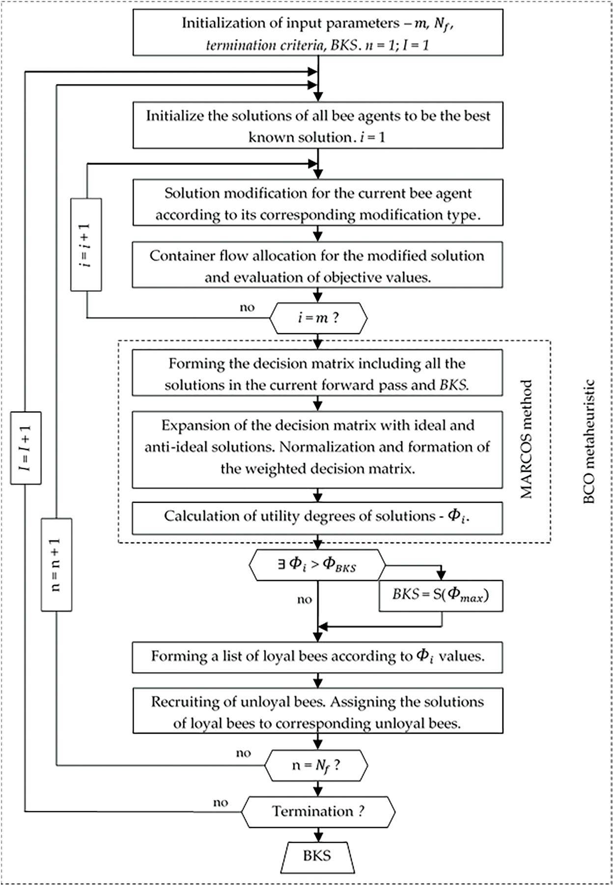
Figure A1: Algorithmic steps of the BCO-MARCOS metaheuristic model