
 Submit a Paper
 Propose a Special lssue
 Open Access
REVIEW

Deep Learning Applied to Computational Mechanics: A Comprehensive Review, State of the Art, and the Classics
1 Aerospace Engineering, University of Illinois at Urbana-Champaign, Champaign, IL 61801, USA
2 Institute of Technical Mechanics, Johannes Kepler University, Linz, A-4040, Austria
* Corresponding Author: Loc Vu-Quoc. Email:
Computer Modeling in Engineering & Sciences 2023, 137(2), 1069-1343. https://doi.org/10.32604/cmes.2023.028130
Received 01 December 2022; Accepted 01 March 2023; Issue published 26 June 2023
 View Full Text
 Download PDF
Abstract
Three recent breakthroughs due to AI in arts and science serve as motivation: An award winning digital image, protein folding, fast matrix multiplication. Many recent developments in artificial neural networks, particularly deep learning (DL), applied and relevant to computational mechanics (solid, fluids, finite-element technology) are reviewed in detail. Both hybrid and pure machine learning (ML) methods are discussed. Hybrid methods combine traditional PDE discretizations with ML methods either (1) to help model complex nonlinear constitutive relations, (2) to nonlinearly reduce the model order for efficient simulation (turbulence), or (3) to accelerate the simulation by predicting certain components in the traditional integration methods. Here, methods (1) and (2) relied on Long-Short-Term Memory (LSTM) architecture, with method (3) relying on convolutional neural networks.. Pure ML methods to solve (nonlinear) PDEs are represented by Physics-Informed Neural network (PINN) methods, which could be combined with attention mechanism to address discontinuous solutions. Both LSTM and attention architectures, together with modern and generalized classic optimizers to include stochasticity for DL networks, are extensively reviewed. Kernel machines, including Gaussian processes, are provided to sufficient depth for more advanced works such as shallow networks with infinite width. Not only addressing experts, readers are assumed familiar with computational mechanics, but not with DL, whose concepts and applications are built up from the basics, aiming at bringing first-time learners quickly to the forefront of research. History and limitations of AI are recounted and discussed, with particular attention at pointing out misstatements or misconceptions of the classics, even in well-known references. Positioning and pointing control of a large-deformable beam is given as an example.Keywords
TABLE OF CONTENTS
1 Opening remarks and organization
2 Deep Learning, resurgence of Artificial Intelligence
2.1 Handwritten equation to LaTeX code, image recognition
2.2 Artificial intelligence, machine learning, deep learning
2.3 Motivation, applications to mechanics
2.3.1 Enhanced numerical quadrature for finite elements
2.3.2 Solid mechanics, multiscale modeling
2.3.3 Fluid mechanics, reduced-order model for turbulence
3 Computational mechanics, neuroscience, deep learning
4 Statics, feedforward networks
4.3 Big picture, composition of concepts
4.3.1 Graphical representation, block diagrams
4.4 Network layer, detailed construct
4.4.1 Linear combination of inputs and biases
4.4.3 Graphical representation, block diagrams
4.5 Representing XOR function with two-layer network
4.6 What is “deep” in “deep networks” ? Size, architecture
5.1 Cost (loss, error) function
5.1.2 Maximum likelihood (probability cost)
5.1.3 Classification loss function
5.2 Gradient of cost function by backpropagation
5.3 Vanishing and exploding gradients
5.3.1 Logistic sigmoid and hyperbolic tangent
5.3.2 Rectified linear function (ReLU)
5.3.3 Parametric rectified linear unit (PReLU)
6 Network training, optimization methods
6.1 Training set, validation set, test set, stopping criteria
6.2 Deterministic optimization, full batch
6.2.2 Inexact line-search, Goldstein’s rule
6.2.3 Inexact line-search, Armijo’s rule
6.2.4 Inexact line-search, Wolfe’s rule
6.3 Stochastic gradient-descent (1st-order) methods
6.3.1 Standard SGD, minibatch, fixed learning-rate schedule
6.3.2 Momentum and fast (accelerated) gradient
6.3.3 Initial-step-length tuning
6.3.4 Step-length decay, annealing and cyclic annealing
6.3.5 Minibatch-size increase, fixed step length, equivalent annealing
6.3.6 Weight decay, avoiding overfit
6.3.7 Combining all add-on tricks
6.5 Adaptive methods: Adam, variants, criticism
6.5.1 Unified adaptive learning-rate pseudocode
6.5.2 AdaGrad: Adaptive Gradient
6.5.3 Forecasting time series, exponential smoothing
6.5.4 RMSProp: Root Mean Square Propagation
6.5.5 AdaDelta: Adaptive Delta (parameter increment)
6.5.7 AMSGrad: Adaptive Moment Smoothed Gradient
6.5.8 AdamX and Nostalgic Adam
6.5.9 Criticism of adaptive methods, resurgence of SGD
6.5.10 AdamW: Adaptive moment with weight decay
6.6 SGD with Armijo line search and adaptive minibatch
6.7 Stochastic Newton method with 2nd-order line search
7 Dynamics, sequential data, sequence modeling
7.1 Recurrent Neural Networks (RNNs)
7.2 Long Short-Term Memory (LSTM) unit
7.3 Gated Recurrent Unit (GRU)
7.4 Sequence modeling, attention mechanisms, Transformer
7.4.1 Sequence modeling, encoder-decoder
7.4.3 Transformer architecture
8 Kernel machines (methods, learning)
8.1 Reproducing kernel: General theory
8.2 Exponential functions as reproducing kernels
8.3.1 Gaussian-process priors and sampling
8.3.2 Gaussian-process posteriors and sampling
9 Deep-learning libraries, frameworks, platforms
9.4 Leveraging DL-frameworks for scientific computing
9.5 Physics-Informed Neural Network (PINN) frameworks
10 Application 1: Enhanced numerical quadrature for finite elements
10.1 Two methods of quadrature, 1-D example
10.2 Application 1.1: Method 1, Optimal number of integration points
10.2.1 Method 1, feasibility study
10.2.2 Method 1, training phase
10.2.3 Method 1, application phase
10.3 Application 1.2: Method 2, optimal quadrature weights
10.3.1 Method 2, feasibility study
10.3.2 Method 2, training phase
10.3.3 Method 2, application phase
11 Application 2: Solid mechanics, multi-scale, multi-physics
11.2 Data-driven constitutive modeling, deep learning
11.3 Multiscale multiphysics problem: Porous media
11.3.1 Recurrent neural networks for scale bridging
11.3.2 Microstructure and principal direction data
11.3.3 Optimal RNN-LSTM architecture
11.3.4 Dual-porosity dual-permeability governing equations
11.3.5 Embedded strong discontinuities, traction-separation law
12 Application 3: Fluids, turbulence, reduced-order models
12.1 Proper orthogonal decomposition (POD)
12.2 POD with LSTM-Reduced-Order-Model
12.2.1 Goal for using neural network
12.2.2 Data generation, training and testing procedure
12.3 Memory effects of POD coefficients on LSTM models
12.4 Reduced order models and hyper-reduction
12.4.1 Motivating example: 1D Burger’s equation
12.4.2 Nonlinear manifold-based (hyper-)reduction
12.4.5 Numerical example: 2D Burger’s equation
13.1 Early inspiration from biological neurons
13.2 Spatial / temporal combination of inputs, weights, biases
13.2.1 Static, comparing modern to classic literature
13.2.2 Dynamic, time dependence, Volterra series
13.3.2 Rectified linear unit (ReLU)
13.4 Back-propagation, automatic differentiation
13.4.2 Automatic differentiation
13.5 Resurgence of AI and current state
13.5.1 COVID-19 machine-learning diagnostics and prognostics
13.5.2 Additional applications of deep learning
14 Closure: Limitations and danger of AI
14.1 Driverless cars, crewless ships, “not any time soon”
14.2 Lack of understanding on why deep learning worked
14.4 Threat to democracy and privacy
14.4.2 Facial recognition nightmare
14.5 AI cannot tackle controversial human problems
14.6 So what’s new? Learning to think like babies
14.7 Lack of transparency and irreproducibility of results
1 Backprop pseudocodes, notation comparison
3 Conditional Gaussian distribution
4 The ups and downs of AI, cybernetics
1 Opening remarks and organization
Breakthroughs due to AI in arts and science. On 2022.08.29, Figure 1, an image generated by the AI software Midjourney, became one of the first of its kind to win first place in an art contest.1 The image author signed his entry to the contest as “Jason M. Allen via Midjourney,” indicating that the submitted digital art was not created by him in the traditional way, but under his text commands to an AI software. Artists not using AI software—such as Midjourney, DALL.E 2, Stable Diffusion—were not happy [4].
In 2021, an AI software achieved a feat that human researchers were not able to do in the last 50 years in predicting protein structures quickly and in a large scale. This feat was named the scientific breakthough of the year; Figure 2, left. In 2016, another AI software beat the world grandmaster in the Go game, which is described as the most complex game that human ever created; Figure 2, right.
On 2022.10.05, DeepMind published a paper on breaking a 50-year record of fast matrix multiplication by reducing the number of multiplications in multiplying two
Since the preprint of this paper was posted on the arXiv in Dec 2022 [9], there have been considerable excitements and concerns about ChatGPT—a large language-model chatbot that can interact with humans in a conversational way—which would be incorporated into Microsoft Bing to make web “search interesting again, after years of stagnation and stasis” [10], whose author wrote “I’m going to do something I thought I’d never do: I’m switching my desktop computer’s default search engine to Bing. And Google, my default source of information for my entire adult life, is going to have to fight to get me back.” Google would release its own answer to ChatGPT called “Bard” [11]. The race is on.

Figure 1: AI-generated image won contest in the category of Digital Arts, Emerging Artists, on 2022.08.29 (Section 1). “Théâtre D’opéra Spatial” (Space Opera Theater) by “Jason M. Allen via Midjourney”, which is “an artificial intelligence program that turns lines of text into hyper-realistic graphics” [4]. Colorado State Fair, 2022 Fine Arts First, Second & Third. (Permission of Jason M. Allen, CEO, Incarnate Games)
Audience. This review paper is written by mechanics practitioners to mechanics practitioners, who may or may not be familiar with neural networks and deep learning. We thus assume that the readers are familiar with continuum mechanics and numerical methods such as the finite element method. Thus, unlike typical computer-science papers on deep learning, notation and convention of tensor analysis familiar to practitioners of mechanics are used here whenever possible.3
For readers not familiar with deep learning, unlike many other review papers, this review paper is not just a summary of papers in the literature for people who already have some familiarity with this topic,4 particularly papers on deep-learning neural networks, but contains also a tutorial on this topic aiming at bringing first-time learners (including students) quickly up-to-date with modern issues and applications of deep learning, especially to computational mechanics.5 As a result, this review paper is a convenient “one-stop shopping” that provides the necessary fundamental information, with clarification of potentially confusing points, for first-time learners to quickly acquire a general understanding of the field that would facilitate deeper study and application to computational mechanics.
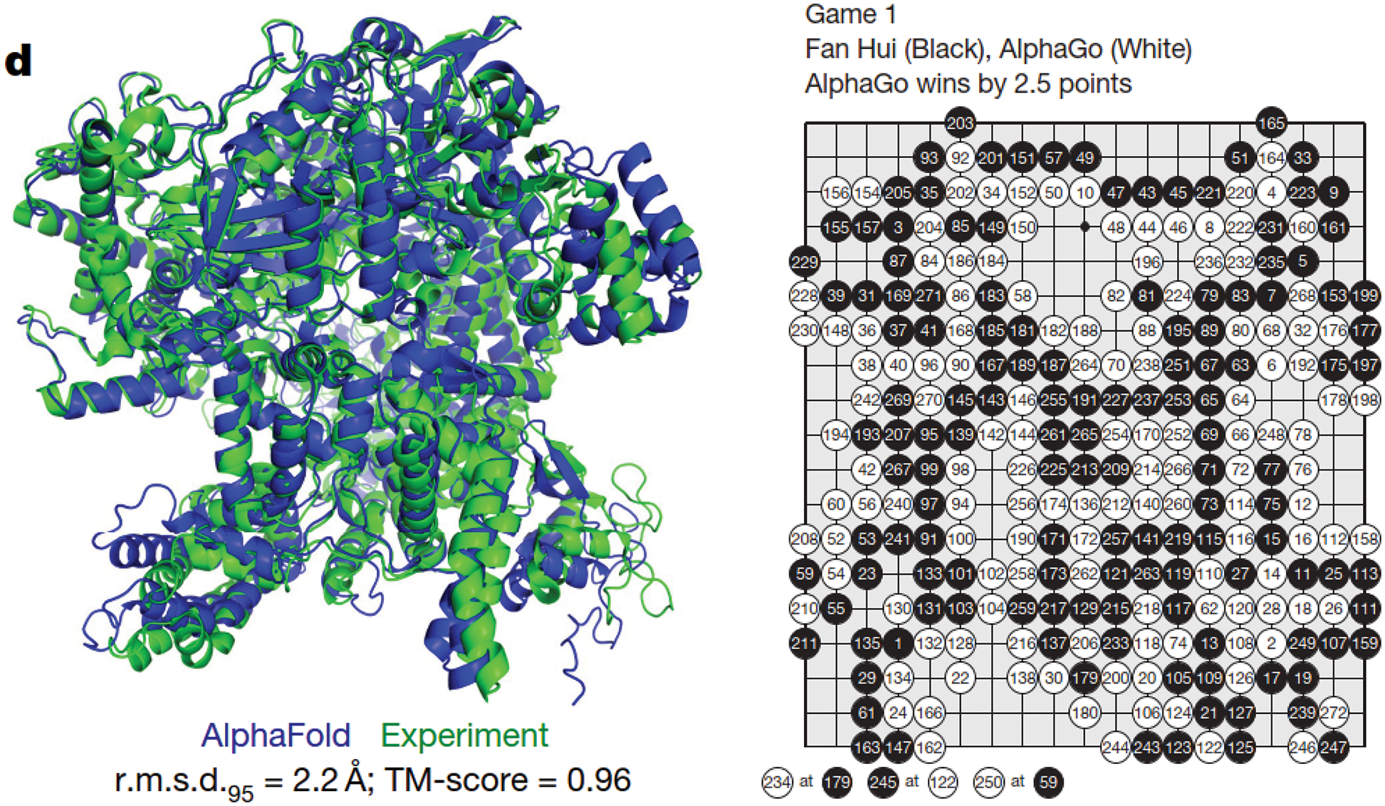
Figure 2: Breakthroughs in AI (Section 2). Left: The journal Science 2021 Breakthough of the Year. Protein folded 3-D shape produced by the AI software AlphaFold compared to experiment with high accuracy [5]. The AlphaFold Protein Structure Database contains more than 200 million protein structure predictions, a holy grail sought after in the last 50 years. Right: The AI solfware AlphaGo, a runner-up in the journal Science 2016 Breakthough of the Year, beat the European Go champion Fan Hui five games to zero in 2015 [6], and then went on to defeat the world Go grandmaster Lee Sedol in 2016 [7]. (Permission by Nature.)
Deep-learning software libraries. Just as there is a large number of available software in different subfields of computational mechanics, there are many excellent deep-learning libraries ready for use in applications; see Section 9, in which some examples of the use of these libraries in engineering applications are provided with the associated computer code. Similar to learning finite-element formulations versus learning how to run finite-element codes, our focus here is to discuss various algorithmic aspects of deep-learning and their applications in computational mechanics, rather than how to use deep-learning libraries in applications. We agree with the view that “a solid understanding of the core principles of neural networks and deep learning” would provide “insights that will still be relevant years from now” [21], and that would not be obtained from just learning to run some hot libraries.
Readers already familiar with neural networks may find the presentation refreshing,6 and even find new information on neural networks, depending how they used deep learning, or when they stopped working in this area due to the waning wave of connectionism and the new wave of deep learning.7 If not, readers can skip these sections to go directly to the sections on applications of deep learning to computational mechanics.
Applications of deep learning in computational mechanics. We select some recent papers on application of deep learning to computational mechanics to review in details in a way that readers would also understand the computational mechanics contents well enough without having to read through the original papers:
• Fully-connected feedforward neural networks were employed to make element-matrix integration more efficient, while retaining the accuracy of the traditional Gauss-Legendre quadrature [38];8
• Recurrent neural network (RNN) with Long Short-Term Memory (LSTM) units9 was applied to multiple-scale, multi-physics problems in solid mechanics [25];
• RNNs with LSTM units were employed to obtain reduced-order model for turbulence in fluids based on the proper orthogonal decomposition (POD), a classic linear project method also known as principal components analysis (PCA) [26]. More recent nonlinear-manifold model-order reduction methods, incorporating encoder / decoder and hyper-reduction of dimentionality using gappy (incomplete) data, were introduced, e.g., [47] [48].
Organization of contents. Our review of each of the above papers is divided into two parts. The first part is to summarize the main results and to identify the concepts of deep learning used in the paper, expected to be new for first-time learners, for subsequent elaboration. The second part is to explain in details how these deep-learning concepts were used to produce the results.
The results of deep-learning numerical integration [38] are presented in Section 2.3.1, where the deep-learning concepts employed are identified and listed, whereas the details of the formulation in [38] are discussed in Section 10. Similarly, the results and additional deep-learning concepts used in a multi-scale, multi-physics problem of geomechanics [25] are presented in Section 2.3.2, whereas the details of this formulation are discussed in Section 11. Finally, the results and additional deep-learning concepts used in turbulent fluid simulation with proper orthogonal decomposition [26] are presented in Section 2.3.3, whereas the details of this formulation, together with the nonlinear-manifold model-order reduction [47] [48], are discussed in Section 12.
All of the deep-learning concepts identified from the above selected papers for in-depth are subsequently explained in detail in Sections 3 to 7, and then more in Section 13 on “Historical perspective”.
The parallelism between computational mechanics, neuroscience, and deep learning is summarized in Section 3, which would put computational-mechanics first-time learners at ease, before delving into the details of deep-learning concepts.
Both time-independent (static) and time-dependent (dynamic) problems are discussed. The architecture of (static, time-independent) feedforward multilayer neural networks in Section 4 is expounded in detail, with first-time learners in mind, without assuming prior knowledge, and where experts may find a refreshing presentation and even new information.
Backpropagation, explained in Section 5, is an important method to compute the gradient of the cost function relative to the network parameters for use as a descent direction to decrease the cost function for network training.
For training networks—i.e., finding optimal parameters that yield low training error and lowest validation error—both classic deterministic optimization methods (using full batch) and stochastic optimization methods (using minibatches) are reviewed in detail, and at times even derived, in Section 6, which would be useful for both first-time learners and experts alike.
The examples used in training a network form the training set, which is complemented by the validation set (to determine when to stop the optimization iterations) and the test set (to see whether the resulting network could work on examples never seen before); see Section 6.1.
Deterministic gradient descent with classical line search methods, such as Armijo’s rule (Section 6.2), were generalized to add stochasticity. Detailed pseudocodes for these methods are provided. The classic stochastic gradient descent (SGD) by Robbins & Monro (1951) [49] (Section 6.3, Section 6.3.1), with add-on tricks such as momentum Polyak (1964) [3] and fast (accelerated) gradient by Nesterov (1983 [50], 2018 [51]) (Section 6.3.2), step-length decay (Section 6.3.4), cyclic annealing (Section 6.3.4), minibatch-size increase (Section 6.3.5), weight decay (Section 6.3.6) are presented, often with detailed derivations.
Step-length decay is shown to be equivalent to simulated annealing using stochastic differential equation equivalent to the discrete parameter update. A consequence is to increase the minibatch size, instead of decaying the step length (Section 6.3.5). In particular, we obtain a new result for minibatch-size increase.
In Section 6.5, highly popular adaptive step-length (learning-rate) methods are discussed in a unified manner in Section 6.5.1, followed by the first paper on AdaGrad [52] (Section 6.5.2).
Overlooked in (or unknown to) other review papers and even well-known books on deep learning, exponential smoothing of time series originating from the field of forecasting dated since the 1950s, the key technique of adaptive methods, is carefully explained in Section 6.5.3.
The first adaptive methods that employed exponential smoothing were RMSProp [53] (Section 6.5.4) and AdaDelta [54] (Section 6.5.5), both introduced at about the same time, followed by the “immensely successful” Adam (Section 6.5.6) and its variants (Sections 6.5.7 and 6.5.8).
Particular attention is then given to a recent criticism of adaptive methods in [55], revealing their marginal value for generalization, compared to the good old SGD with effective initial step-length tuning and step-length decay (Section 6.5.9). The results were confirmed in three recent independent papers, among which is the recent AdamW adaptive method in [56] (Section 6.5.10).
Dynamics, sequential data, and sequence modeling are the subjects of Section 7. Discrete time-dependent problems, as a sequence of data, can be modeled with recurrent neural networks discussed in Section 7.1, using the 1997 classic architecture such as Long Short-Term Memory (LSTM) in Section 7.2, but also the recent 2017-18 architectures such as transformer introduced in [31] (Section 7.4.3), based on the concept of attention [57]. Continuous recurrent neural networks originally developed in neuroscience to model the brain and the connection to their discrete counterparts in deep learning are also discussed in detail, [19] and Section 13.2.2 on “Dynamic, time dependence, Volterra series”.
The features of several popular, open-source deep-learning frameworks and libraries—such as TensorFlow, Keras, PyTorch, etc.—are summarized in Section 9.
As mentioned above, detailed formulations of deep learning applied to computational mechanics in [38] [25] [26] [47] [48] are reviewed in Sections 10, 11, 12.
History of AI, limitations, danger, and the classics. Finally, a broader historical perspective of deep learning, machine learning, and artificial intelligence is discussed in Section 13, ending with comments on the geopolitics, limitations, and (identified-and-proven, not just speculated) danger of artificial intelligence in Section 14.
A rare feature is in a detailed review of some important classics to connect to the relevant concepts in modern literature, sometimes revealing misunderstanding in recent works, likely due to a lack of verification of the assertions made with the corresponding classics. For example, the first artificial neural network, conceived by Rosenblatt (1957) [1], (1962) [2], had 1000 neurons, but was reported as having a single neuron (Figure 42). Going beyond probabilistic analysis, Rosenblatt even built the Mark I computer to implement his 1000-neuron network (Figure 133, Sections 13.2 and 13.2.1). Another example is the “heavy ball” method, for which everyone referred to Polyak (1964) [3], but who more precisely called the “small heavy sphere” method (Remark 6.6). Others were quick to dismiss classical deterministic line-search methods that have been generalized to add stochasticity for network training (Remark 6.4). Unintended misrepresentation of the classics would mislead first-time learners, and unfortunately even seasoned researchers who used second-hand information from others, without checking the original classics themselves.
The use of Volterra series to model the nonlinear behavior of neuron in term of input and output firing rates, leading to continuous recurrent neural networks is examined in detail. The linear term of the Volterra series is a convolution integral that provides a theoretical foundation for the use of linear combination of inputs to a neuron, with weights and biases [19]; see Section 13.2.2.
The experiments in the 1950s by Furshpan et al. [58] [59] that revealed the rectified linear behavior in neuronal axon, modeled as a circuit with a diode, together with the use of the rectified linear activation function in neural networks in neuroscience years before being adopted for use in deep learning network, are reviewed in Section 13.3.2.
Reference hypertext links and Internet archive. For the convenience of the readers, whenever we refer to an online article, we provide both the link to original website, and if possible, also the link to its archived version in the Internet Archive. For example, we included in the bibliography entry of Ref. [60] the links to both the Original website and the Internet archive.10
2 Deep Learning, resurgence of Artificial Intelligence
In Dec 2021, the journal Science named, as its “2021 Breakthrough of the Year,” the development of the AI software AlphaFold and its amazing feat of predicting a large number of protein structures [64]. “For nearly 50 years, scientists have struggled to solve one of nature’s most perplexing challenges—predicting the complex 3D shape a string of amino acids will twist and fold into as it becomes a fully functional protein. This year, scientists have shown that artificial intelligence (AI)-driven software can achieve this long-standing goal and predict accurate protein structures by the thousands and at a fraction of the time and cost involved with previous methods” [64].
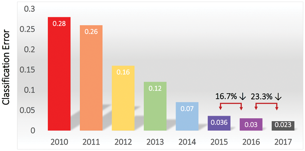
Figure 3: ImageNet competitions (Section 2). Top (smallest) classification error rate versus competition year. A sharp decrease in error rate in 2012 sparked a resurgence in AI interest and research [13]. By 2015, the top classification error rate surpassed human classification error rate of 5.1% with Parametric Rectified Linear Unit [61]; see Section 5.3.3 and also [62]. Figure from [63]. (Figure reproduced with permission of the authors.)
The 3-D shape of a protein, obtained by folding a linear chain of amino acid, determines how this protein would interact with other molecules, and thus establishes its biological functions [64]. There are some 200 million proteins, the building blocks of life, in all living creatures, and 400,000 in the human body [64]. The AlphaFold Protein Structure Database already contained “over 200 million protein structure predictions.”11 For comparison, there were only about 190 thousand protein structures obtained through experiments as of 2022.07.28 [65]. “Some of AlphaFold’s predictions were on par with very good experimental models [Figure 2, left], and potentially precise enough to detail atomic features useful for drug design, such as the active site of an enzyme” [66]. The influence of this software and its developers “would be epochal.”
On the 2019 new-year day, The Guardian [67] reported the most recent breakthrough in AI, published less than a month before on 2018 Dec 07 in the journal Science in [68] on the development of the software AlphaZero, based on deep reinforcement learning (a combination of deep learning and reinforcement learning), that can teach itself through self-play, and then “convincingly defeated a world champion program in the games of chess, shogi (Japanese chess), as well as Go”; see Figure 2, right.
Go is the most complex game that mankind ever created, with more combinations of possible moves than chess, and thus the number of atoms in the observable universe.12 It is “the most challenging of classic games for artificial intelligence [AI] owing to its enormous search space and the difficulty of evaluating board positions and moves” [6].
This breakthrough is the crowning achievement in a string of astounding successes of deep learning (and reinforcenent learning) in taking on this difficult challenge for AI.13 The success of this recent breakthrough prompted an AI expert to declare close the multidecade long, arduous chapter of AI research to conquer immensely-complex games such as chess, shogi, and Go, and to suggest AI researchers to consider a new generation of games to provide the next set of challenges [73].
In its long history, AI research went through several cycles of ups and downs, in and out of fashion, as described in [74], ‘Why artificial intelligence is enjoying a renaissance’ (see also Section 13 on historical perspective):
“THE TERM “artificial intelligence” has been associated with hubris and disappointment since its earliest days. It was coined in a research proposal from 1956, which imagined that significant progress could be made in getting machines to “solve kinds of problems now reserved for humans if a carefully selected group of scientists work on it together for a summer”. That proved to be rather optimistic, to say the least, and despite occasional bursts of progress and enthusiasm in the decades that followed, AI research became notorious for promising much more than it could deliver. Researchers mostly ended up avoiding the term altogether, preferring to talk instead about “expert systems” or “neural networks”. But in the past couple of years there has been a dramatic turnaround. Suddenly AI systems are achieving impressive results in a range of tasks, and people are once again using the term without embarrassment.”
The recent resurgence of enthusiasm for AI research and applications dated only since 2012 with a spectacular success of almost halving the error rate in image classification in the ImageNet competition,14 Going from 26% down to 16%; Figure 3 [63]. In 2015, deep-learning error rate of 3.6% was smaller than human-level error rate of 5.1%,15 and then decreased by more than half to 2.3% by 2017.
The 2012 success16 of a deep-learning application, which brought renewed interest in AI research out of its recurrent doldrums known as “AI winters”,17 is due to the following reasons:
• Availability of much larger datasets for training deep neural networks (find optimized parameters). It is possible to say that without ImageNet, there would be no spectacular success in 2012, and thus no resurgence of AI. Once the importance of having large datasets to develop versatile, working deep networks was realized, many more large datasets have been developed. See, e.g., [60].
• Emergence of more powerful computers than in the 1990s, e.g., the graphical processing unit (or GPU), “which packs thousands of relatively simple processing cores on a single chip” for use to process and display complex imagery, and to provide fast actions in today’s video games” [77].
• Advanced software infrastructure (libraries) that facilitates faster development of deep-learning applications, e.g., TensorFlow, PyTorch, Keras, MXNet, etc. [78], p. 25. See Section 9 on some reviews and rankings of deep-learning libraries.
• Larger neural networks and better training techniques (i.e., optimizing network parameters) that were not available in the 1980s. Today’s much larger networks, which can solve once intractatable / difficult problems, are “one of the most important trends in the history of deep learning”, but are still much smaller than the nervous system of a frog [78], p. 21; see also Section 4.6. A 2006 breakthrough, ushering in the dawn of a new wave of AI research and interest, has allowed for efficient training of deeper neural networks [78], p. 18.18 The training of large-scale deep neural networks, which frequently involve highly nonlinear and non-convex optimization problems with many local minima, owes its success to the use of stochastic-gradient descent method first introduced in the 1950s [80].
• Successful applications to difficult, complex problems that help people in their every-day lives, e.g., image recognition, speech translation, etc.
Section 13 provices a historical perspective on the development of AI, with additional details on current and future applications.
It was, however, disappointing that despite the above-mentioned exciting outcomes of AI, during the Covid-19 pandemic beginning in 2020,23 none of the hundreds of AI systems developed for Covid-19 diagnosis were usable for clinical applications; see Section 13.5.1. As of June 2022, the Tesla electric vehicle autopilot system is under increased scrutiny by the National Highway Traffic Safety Administration as there were “16 crashes into emergency vehicles and trucks with warning signs, causing 15 injuries and one death.”24 In addition, there are many limitations and danger in the current state-of-the-art of AI; see Section 14.
2.1 Handwritten equation to LaTeX code, image recognition
An image-recognition software useful for computational mechanicists is Mathpix Snip,25 which recognizes hand-written math equations, and transforms them into LaTex codes. For example, Mathpix Snip transforms the hand-written equation below by an 11-year old pupil:
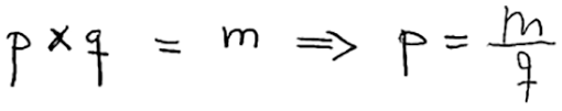
Figure 4: Handwritten equation 1 (Section 2.1)
into this LaTeX code “p \times q = m \Rightarrow p = \frac { m } { q }” to yield the equation image:
Another example is the hand-written multiplication work below by the same pupil:
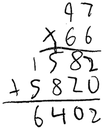
Figure 5: Handwritten equation 2 (Section 2.1). Hand-written multiplication work of an eleven-year old pupil.
that Mathpix Snip transformed into the equation image below:26
2.2 Artificial intelligence, machine learning, deep learning
We want to immediately clarify the meaning of the terminologies “Artificial Intelligence” (AI), “Machine Learning” (ML), and “Deep Learning” (DL), since their casual use could be confusing for first-time learners.
For example, it was stated in a review of primarily two computer-science topics called “Neural Networks” (NNs) and “Support Vector Machines” (SVMs) and a physics topic that [85]:27
“The respective underlying fields of basic research—quantum information versus machine learning (ML) and artificial intelligence (AI)—have their own specific questions and challenges, which have hitherto been investigated largely independently.”
Questions would immediately arise in the mind of first-time learners: Are ML and AI two different fields, or the same fields with different names? If one field is a subset of the other, then would it be more general to just refer to the larger set? On the other hand, would it be more specific to just refer to the subset?
In fact, Deep Learning is a subset of methods inside a larger set of methods known as Machine Learning, which in itself is a subset of methods generally known as Artificial Intelligence. In other words, Deep Learning is Machine Learning, which is Artificial Intelligence; [78], p. 9.28 On the other hand, Artificial Intelligence is not necessarily Machine Learning, which in itself is not necessarily Deep Learning.
The review in [85] was restricted to Neural Networks (which could be deep or shallow)29 and Support Vector Machine (which is Machine Learning, but not Deep Learning); see Figure 6. Deep Learning can be thought of as multiple levels of composition, going from simpler (less abstract) concepts (or representations) to more complex (abstract) concepts (or representations).30
Based on the above relationship between AI, ML, and DL, it would be much clearer if the phrase “machine learning (ML) and artificial intelligence (AI)” in both the title of [85] and the original sentence quoted above is replaced by the phrase “machine learning (ML)” to be more specific, since the authors mainly reviewed Multi-Layer Neural (MLN) networks (deep learning, and thus machine learning) and Support Vector Machine (machine learning).31 MultiLayer Neural (MLN) network is also known as MultiLayer Perceptron (MLP).32 both MLN networks and SVMs are considered as artificial intelligence, which in itself is too broad and thus not specific enough.
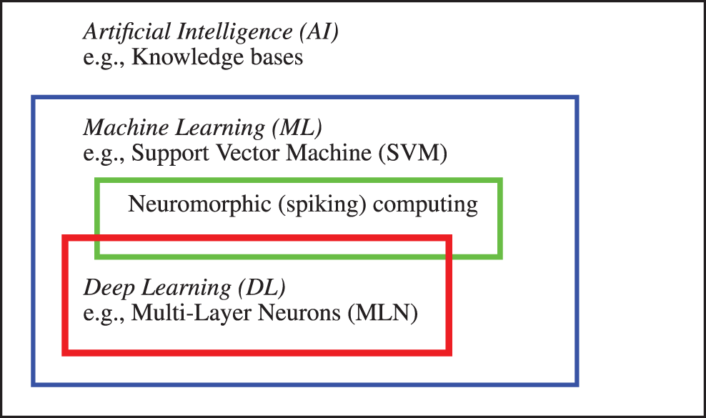
Figure 6: Artificial intelligence and subfields (Section 2.2). Three classes of methods—Artificial Intelligence (AI), Machine Learning (ML), and Deep Learning (DL)—and their relationship, with an example of method in each class. A knowledge-base method is an AI method, but is neither a ML method, nor a DL method. Support Vector Machine and spiking computing are ML methods, and thus AI methods, but not a DL method. Multi-Layer Neural (MLN) network is a DL method, and is thus both an ML method and an AI method. See also Figure 158 in Appendix 4 on Cybernetics, which encompassed all of the above three classes.
Another reason for simplifying the title in [85] is that the authors did not consider using any other AI methods, except for two specific ML methods, even though they discussed AI in the general historical context.
The engine of neuromorphic computing, also known as spiking computing, is a hardware network built into the IBM TrueNorth chip, which contains “1 million programmable spiking neurons and 256 million configurable synapses”,33 and consumes “extremely low power” [87]. Despite the apparent difference with the software approach of deep computing, neuromorphic chip could implement deep-learning networks, and thus the difference was not fundamental [88]. There is thus an overlap between neuromorphic computing and deep learning, as shown in Figure 6, instead of two disconnected subfields of machine learning as reported in [20].34
2.3 Motivation, applications to mechanics
As motivation, we present in this section the results in three recent papers in computational mechanics, mentioned in the Opening Remarks in Section 1, and identify some deep-learning fundamental concepts (in italics) employed in these papers, together with the corresponding sections in the present paper where these concepts are explained in detail. First-time learners of deep learning likely find these fundamental concepts described by obscure technical jargon, whose meaning will be explained in details in the identified subsequent sections. Experts of deep learning would understand how deep learning is applied to computational mechanics.
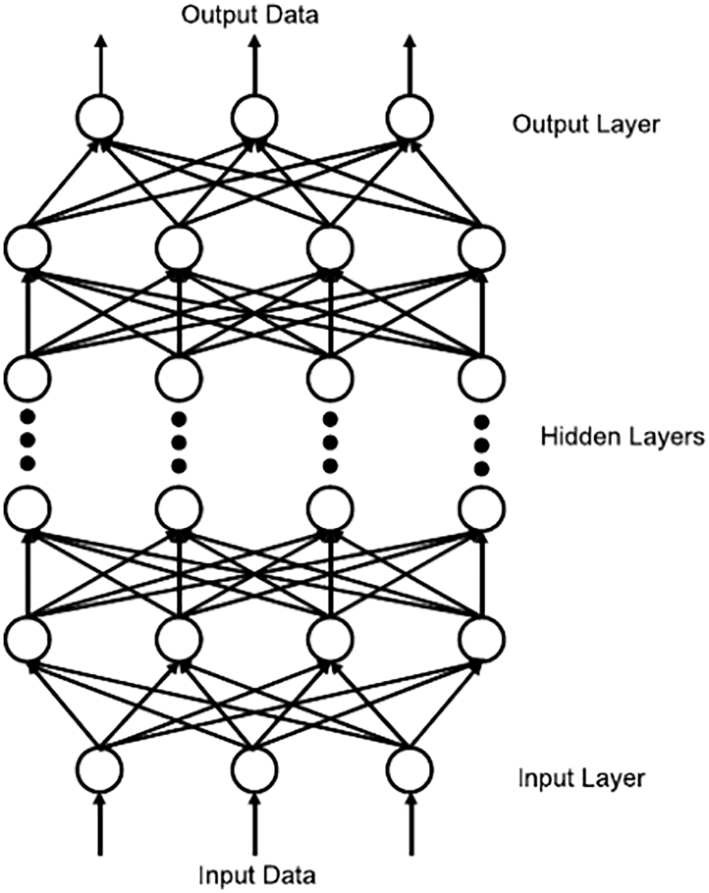
Figure 7: Feedforward neural network (Section 2.3.1). A feedforward neural network in [38], rotated clockwise by 90 degrees to compare to its equivalent in Figure 23 and Figure 35 further below. All terminologies and fundamental concepts will be explained in detail in subsequent sections as listed. See Section 4.1.1 for a top-down explanation and Section 4.1.2 for bottom-up explanation. This figure of a network could be confusing to first-time learners, as already indicated in Footnote 5. (Figure reproduced with permission of the authors.)
2.3.1 Enhanced numerical quadrature for finite elements
To integrate efficiently and accurately the element matrices in a general finite element mesh of 3-D hexahedral elements (including distorted elements), the power of Deep Learning was harnessed in two applications of feedforward MultiLayer Neural networks (MLN,35 Figures 7-8, Section 4) [38]:
(1) Application 1.1: For each element (particularly distorted elements), find the number of integration points that provides accurate integration within a given error tolerance. Section 10.2 contains the details.
(2) Application 1.2: Uniformly use
To train37 the networks—i.e., to optimize the network parameters (weights and biases, Figure 8) to minimize some loss (cost, error) function (Sections 5.1, 6)—up to 20000 randomly distorted hexahedrals were generated by displacing nodes from a regularly shaped element [38], see Figure 9. For each distorted shape, the following are determined: (1) the minimum number of integration points required to reach a prescribed accuracy, and (2) corrections to the quadrature weights by trying one million randomly generated sets of correction factors, among which the best one was retained.
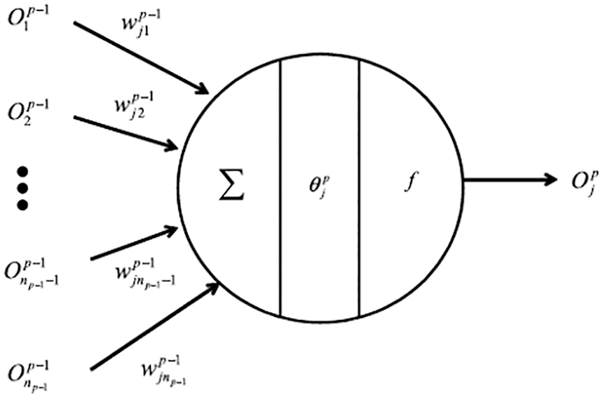
Figure 8: Artificial neuron (Section 2.3.1). A neuron with its multiple inputs
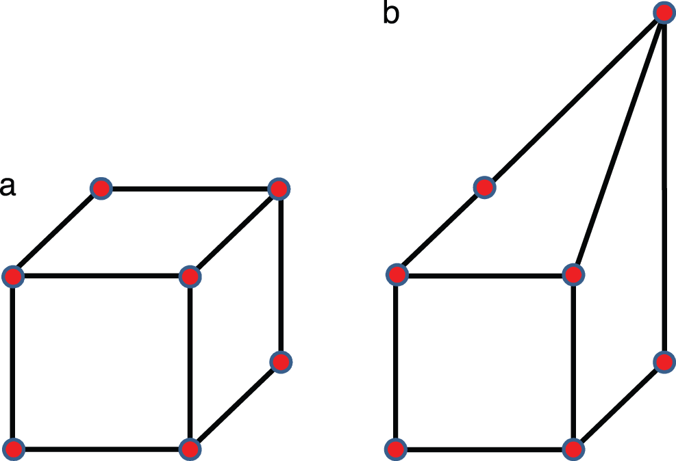
Figure 9: Cube and distorted cube elements (Section 2.3.1). Regular and distorted linear hexahedral elements [38]. (Figure reproduced with permission of the authors.)
While Application 1.1 used one fully-connected (Section 4.6.1) feedforward neural network (Section 4), Application 1.2 relied on two neural networks: The first neural network was a classifier that took the element shape (18 normalized nodal coordinates) as input and estimated whether or not the numerical integration (quadrature) could be improved by adjusting the quadrature weights for the given element (one output), i.e., the network classifier only produced two outcomes, yes or no. If an error reduction was possible, a second neural network performed regression to predict the corrected quadrature weights (eight outputs for
To train the classifier network, 10,000 element shapes were selected from the prepared dataset of 20,000 hexahedrals, which were divided into a training set and a validation set (Section 6.1) of 5000 elements each.38
To train the second regression network, 10,000 element shapes were selected for which quadrature could be improved by adjusting the quadrature weights [38].
Again, the training set and the test set comprised 5000 elements each. The parameters of the neural networks (weights, biases, Figure 8, Section 4.4) were optimized (trained) using a gradient descent method (Section 6) that minimizes a loss function (Section 5.1), whose gradients with respect to the parameters are computed using backpropagation (Section 5).
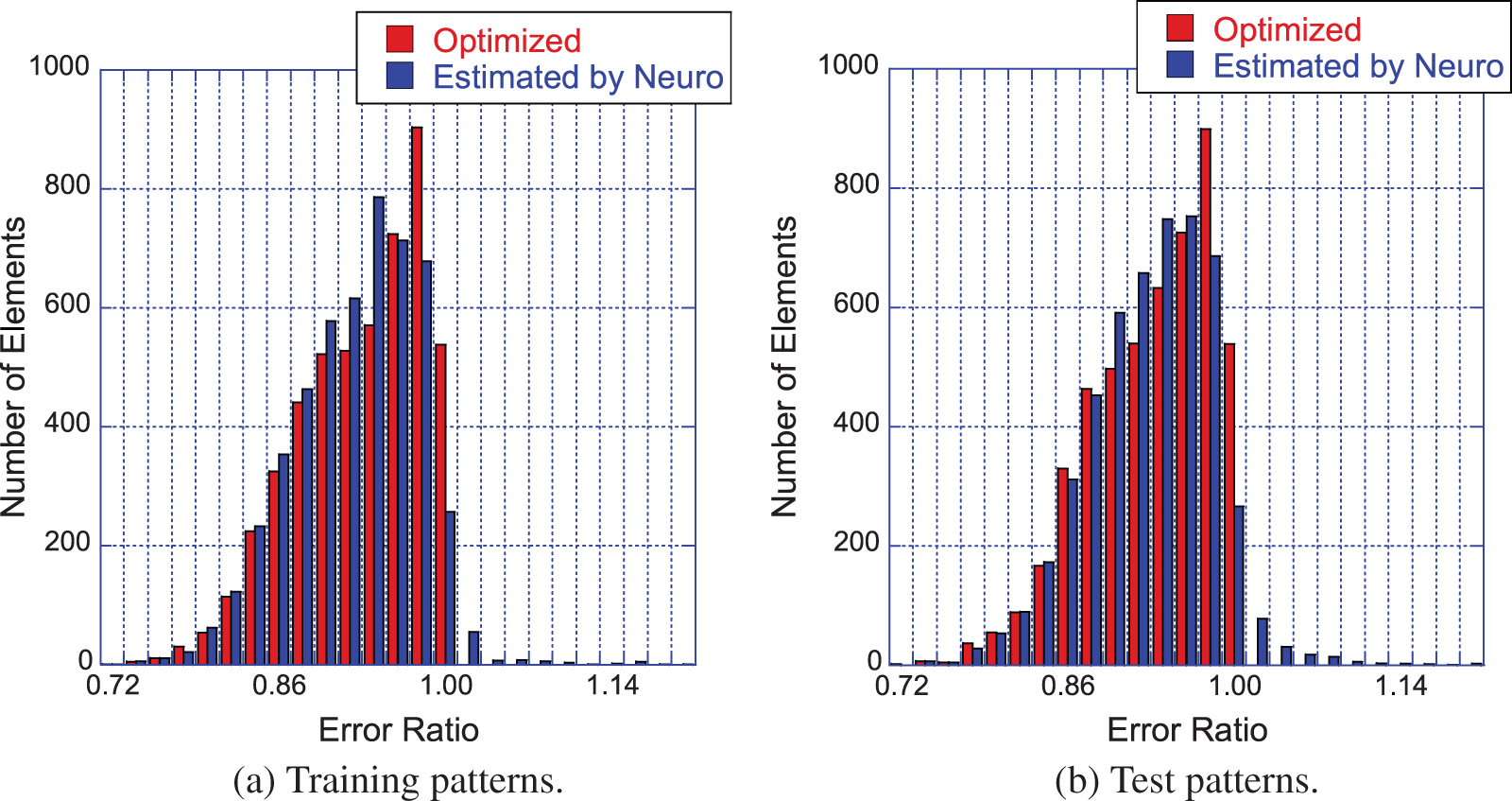
Figure 10: Effectiveness of quadrature weight prediction (Section 2.3.1). Subfigure (a): Distribution of error-reduction ratio
The best results were obtained from a classifier with four hidden layers (Figure 7, Section 4.3, Remark 4.2) with 30 neurons (Figure 8, Figure 36, Section 4.4.3) each and a regression network that had a depth of five hidden layers, where each layer was 50 neurons wide, Figure 7. The results were obtained using the logistic sigmoid function (Figure 30) as activation function (Section 4.4.2) due to existing software, even though the rectified linear function (Figure 24) were more efficient, but yielded comparable accuracy on a few test cases.39
To quantify the effectiveness of the approach in [38], an error-reduction ratio was introduced, i.e., the quotient of the quadrature error with quadrature weights predicted by the neural network and the error obtained with the standard quadrature weights of Gauss-Legendre quadrature with
For most element shapes of both the training set (a) and the test set (b), each of which comprised 5000 elements, the blue bars in Figure 10 indicate an error ratio below one, i.e., the quadrature weight correction effectively improved the accuracy of numerical quadrature.
Readers familiar with Deep Learning and neural networks can go directly to Section 10, where the details of the formulations in [38] are presented. Other sections are also of interest such as classic and state-of-the-art optimization methods in Section 6, attention and transformer unit in Section 7, historical perspective in Section 13, limitations and danger of AI in Section 14.
Readers not familiar with Deep Learning and neural networks will find below a list of the concepts that will be explained in subsequent sections. To facilitate the reading, we also provide the section number (and the link to jump to) for each concept.
Deep-learning concepts to explain and explore:
(1) Feedforward neural network (Figure 7): Figure 23 and Figure 35, Section 4
(2) Neuron (Figure 8): Figure 36 in Section 4.4.4 (artificial neuron), and Figure 131 in Section 13.1 (biological neuron)
(3) Inputs, output, hidden layers, Section 4.3
(4) Network depth and width: Section 4.3
(5) Parameters, weights, biases 4.4.1
(6) Activation functions: Section 4.4.2
(7) What is “deep” in “deep networks” ? Size, architecture, Section 4.6.1, Section 4.6.2
(8) Backpropagation, computation of gradient: Section 5
(9) Loss (cost, error) function, Section 5.1
(10) Training, optimization, stochastic gradient descent: Section 6
(11) Training error, validation error, test (or generalization) error: Section 6.1
This list is continued further below in Section 2.3.2. Details of the formulation in [38] are discussed in Section 10.
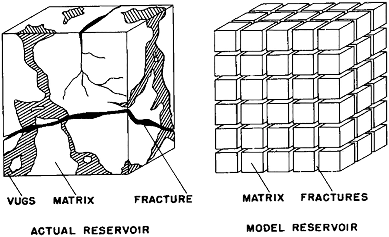
Figure 11: Dual-porosity single-permeability medium (Section 2.3.2). Left: Actual reservoir. Dual (or double) porosity indicates the presence of two types of porosity in naturally-fractured reservoirs (e.g., of oil): (1) Primary porosity in the matrix (e.g., voids in sands) with low permeability, within which fluid does not flow, (2) Secondary porosity due to fractures and vugs (cavities in rocks) with high (anisotropic) permeability, within which fluid flows. Fluid exchange is permitted between the matrix and the fractures, but not between the matrix blocks (sugar cubes), of which the permeability is much smaller than in the fractures. Right: Model reservoir, idealization. The primary porosity is an array of cubes of homogeneous, isotropic material. The secondary porosity is an “orthogonal system of continuous, uniform fractures”, oriented along the principal axes of anisotropic permeability [89]. (Figure reproduced with permission of the publisher SPE.)
2.3.2 Solid mechanics, multiscale modeling
One way that deep learning can be used in solid mechanics is to model complex, nonlinear constitutive behavior of materials. In single physics, balance of linear momentum and strain-displacement relation are considered as definitions or “universal principles”, leaving the constitutive law, or stress-strain relation, to a large number of models that have limitations, no matter how advanced [91]. Deep learning can help model complex constitutive behaviors in ways that traditional phenomenological models could not; see Figure 105.
Deep recurrent neural networks (RNNs) (Section 7.1) was used as a scale-bridging method to efficiently simulate multiscale problems in hydromechanics, specifically plasticity in porous media with dual porosity and dual permeability [25].40
The dual-porosity single-permeability (DPSP) model was first introduced for use in oil-reservoir simulation [89], Figure 11, where the fracture system was the main flow path for the fluid (e.g., two phase oil-water mixture, one-phase oil-solvent mixture). Fluid exchange is permitted between the rock matrix and the fracture system, but not between the matrix blocks. In the DPSP model, the fracture system and the rock matrix, each has its own porosity, with values not differing from each other by a large factor. On the contrary, the permeability of the fracture system is much larger than that in the rock matrix, and thus the system is considered as having only a single permeability. When the permeability of the fracture system and that of the rock matrix do not differ by a large factor, then both permeabilities are included in the more general dual-porosity dual-permeability (DPDP) model [94].
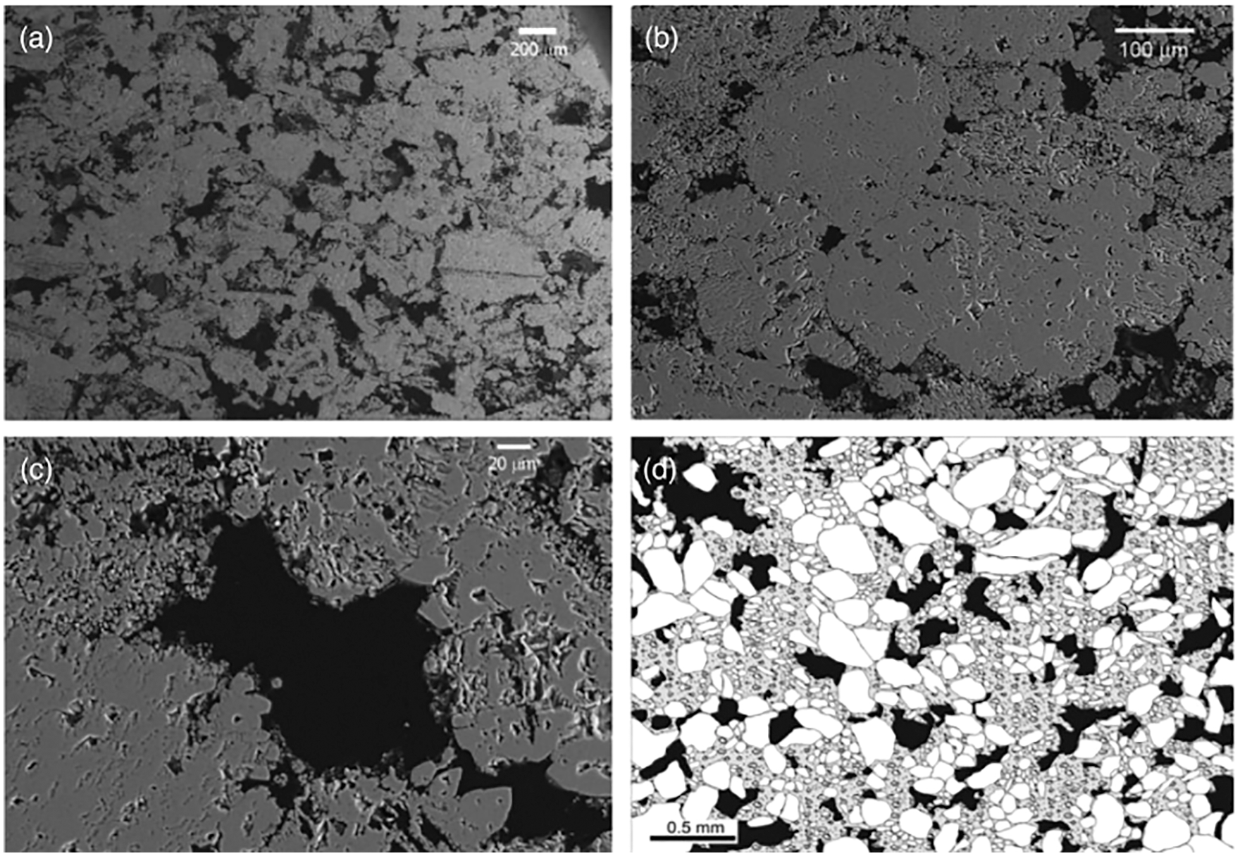
Figure 12: Pore structure of Majella limestone, dual porosity (Section 2.3.2), a carbonate rock with high total porisity at 30%. Backscattered SEM images of Majella limestone: (a)-(c) sequence of zoomed-ins; (d) zoomed-out. (a) The larger macropores (dark areas) have dimensions comparable to the grains (allochems), having an average diameter of 54
Since 60% of the world’s oil reserve and 40% of the world’s gas reserve are held in carbonate rocks, there has been a clear interest in developing an understanding of the mechanical behavior of carbonate rocks such as limestones, having from lowest porosity (Solenhofen at 3%) to high porosity (e.g., Majella at 30%). Chalk (Lixhe) is a carbonate rock with highest porosity at 42.8%. Carbonate rock reservoirs are also considered to store carbon dioxide and nuclear waste [95] [93].
In oil-reservoir simulations in which the primary interest is the flow of oil, water, and solvent, the porosity (and pore size) within each domain (rock matrix or fracture system) is treated as constant and homogeneous [94] [96].41 On the other hand, under mechanical stress, the pore size would change, cracks and other defects would close, leading to a change in the porosity in carbonate rocks. Indeed, “at small stresses, experimental mechanical deformation of carbonate rock is usually characterized by a non-linear stress-strain relationship, interpreted to be related to the closure of cracks, pores, and other defects. The non-linear stress-strain relationship can be related to the amount of cracks and various type of pores” [95], p. 202. Once the pores and cracks are closed, the stress-strain relation becomes linear, at different stress stages, depending on the initial porosity and the geometry of the pore space [95].
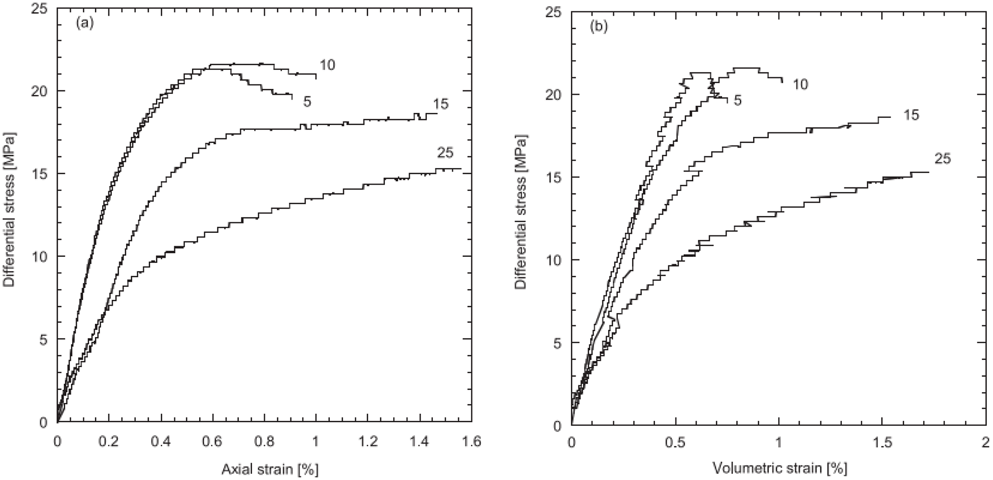
Figure 13: Majella limestone, nonlinear stress-strain relations (Section 2.3.2). Differential stress (i.e., the difference between the largest principal stress and the smallest one) vs axial strain (left) and vs volumetric strain (right) [90]. See Remark 11.7, Section 11.3.4, and Remark 11.10, Section 11.3.5. (Figure reproduced with permission of the authors.)
Moreover, pores have different sizes, and can be classified into different pore sub-systems. For the Majella limestone in Figure 12 with total porosity at 30%, its pore space can be partitioned into two subsystems (and thus dual porosity), the macropores with macroporosity at 11.4% and the micropores with microporosity at 19.6%. Thus the meaning of dual-porosity as used in [25] is different from that in oil-reservoir simulation. Also characteristic of porous rocks such as the Majella limestone is the non-linear stress-strain relation observed in experiments, Figure 13, due the changing size, and collapse, of the pores.
Likewise, the meaning of “dual permeability” is different in [25] in the sense that “one does not seek to obtain a single effective permeability for the entire pore space”. Even though it was not explicitly spelled out,42 it appears that each of the two pore sub-systems would have its own permeability, and that fluid is allowed to exchange between the two pore sub-systems, similar to the fluid exchange between the rock matrix and the fracture system in the DPSP and DPDP models in oil-reservoir simulation [94].
In the problem investigated in [25], the presence of localized discontinuities demands three scales—microscale (
Instead of coupling multiple simulation models online, two (adjacent) scales were linked by a neural network that was trained offline using data generated by simulations on the smaller scale [25]. The trained network subsequently served as a surrogate model in online simulations on the larger scale. With three scales being considered, two recurrent neural networks (RNNs) with Long Short-Term Memory (LSTM) units were employed consecutively:
(1) Mesoscale RNN with LSTM units: On the microscopic scale, a representative volume element (RVE) was an assembly of discrete-element particles, subjected to large variety of representative loading paths to generate training data for the supervised learning of the mesoscale RNN with LSTM units, a neural network that was referred to as “Mesoscale data-driven constitutive model” [25] (Figure 14). Homogenizing the results of DEM-flow model provided constitutive equations for the traction-separation law and the evolution of anisotropic permeabilities in damaged regions.
(2) Macroscale RNN with LSTM units: The mesoscale RVE (middle row in Figure 14), in turn, was a finite-element model of a porous material with embedded strong discontinuities equivalent to the fracture system in oil-reservoir simulation in Figure 11. The host matrix of the RVE was represented by an isotropic linearly elastic solid. In localized fracture zones within, the traction-separation law and the hydraulic response were provided by the mesoscale RNN with LSTM units developed above. Training data for the macroscale RNN with LSTM units—a network referred to as “Macroscale data-driven constitutive model” [25]—is generated by computing the (homogenized) response of the mesoscale RVE to various loadings. In macroscopic simulations, the mesoscale RNN with LSTM units provided the constitutive response at a sealing fault that represented a strong discontinuity.
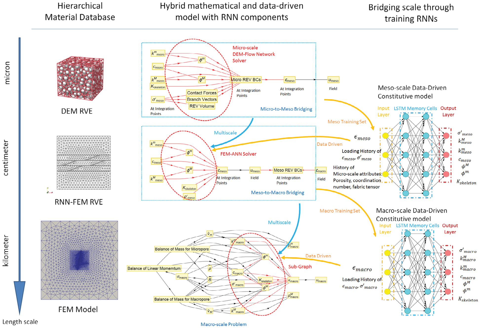
Figure 14: Hierarchy of a multi-scale multi-physics poromechanics problem for fluid-infiltrating media [25] (Sections 2.3.2, 11.1, 11.3.1, 11.3.3, 11.3.5). Microscale (
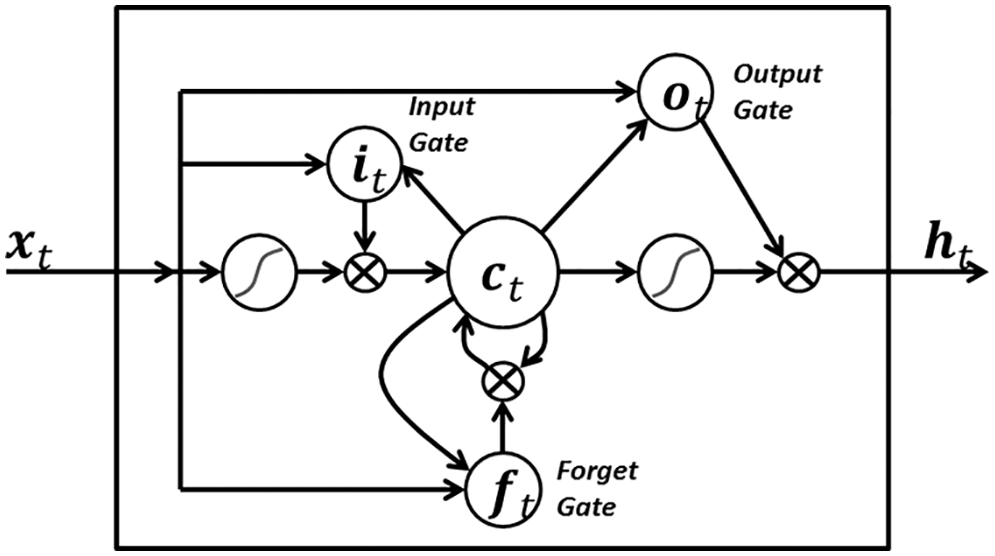
Figure 15: LSTM variant with “peephole” connections, block diagram (Sections 2.3.2, 7.2).43 Unlike the original LSTM unit (see Section 7.2), both the input gate and the forget gate in an LSTM unit with peephole connections receive the cell state as input. The above figure from Wikipedia, version 22:56, 4 October 2015, is identical to Figure 10 in [25], whose authors erroneously used this figure without mentioning the source, but where the original LSTM unit without “peepholes” was actually used, and with the detailed block diagram in Figure 81, Section 7.2. See also Figure 82 and Figure 117 for the original LSTM unit applied to fluid mechanics. (CC-BY-SA 4.0)
Path-dependence is a common characteristic feature of the constitutive models that are often realized as neural networks; see, e.g., [23]. For this reason, it was decided to employ RNN with LSTM units, which could mimick internal variables and corresponding evolution equations that were intrinsic to path-dependent material behavior [25]. These authors chose to use a neural network that had a depth of two hidden layers with 80 LSTM units per layer, and that had proved to be a good compromise of performance and training efforts. After each hidden layer, a dropout layer with a dropout rate 0.2 were introduced to reduce overfitting on noisy data, but yielded minor effects, as reported in [25]. The output layer was a fully-connected layer with a logistic sigmoid as activation function.
An important observation is that including micro-structural data—the porosity
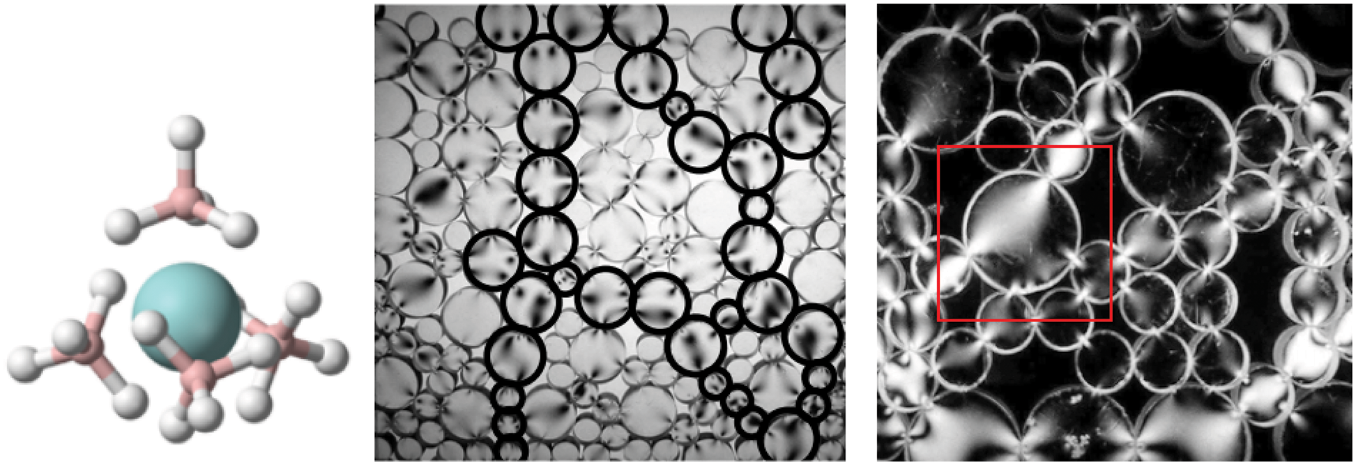
Figure 16: Coordination number CN (Section 2.3.2, 11.3.2). (a) Chemistry. Number of bonds to the central atom. Uranium borohydride U(BH4)4 has CN = 12 hydrogen bonds to uranium. (b, c) Photoelastic discs showing number of contact points (coordination number) on a particle. (b) Random packing and force chains, different force directions along principal chains and in secondary particles. (c) Arches around large pores, precarious stability around pores. The coordination number for the large disc (particle) in red square is 5, but only 4 of those had nonzero contact forces based on the bright areas showing stress action. Figures (b, c) also provide a visualization of the “flow” of the contact normals, and thus the fabric tensor [98]. See also Figure 17. (Figure reproduced with permission of the author.)
Figure 17 illustrates the importance of incorporating microstructure data, particularly the fabric tensor, in network training to improve prediction accuracy.
Deep-learning concepts to explain and explore: (continued from above in Section 2.3.1)
(12) Recurrent neural network (RNN), Section 7.1
(13) Long Short-Term Memory (LSTM), Section 7.2
(14) Attention and Transformer, Section 7.4.3
(15) Dropout layer and dropout rate,45 which had minor effects in the particular work repoorted in [25], and thus will not be covered here. See [78], p. 251, Section 7.12.
Details of the formulation in [25] are discussed in Section 11.
2.3.3 Fluid mechanics, reduced-order model for turbulence
The accurate simulation of turbulence in fluid flows ranks among the most demanding tasks in computational mechanics. Owing to both the spatial and the temporal resolution, transient analysis of turbulence by means of high-fidelity methods such as Large Eddy Simulation (LES) or direct numerical simulation (DNS) involves millions of unknowns even for simple domains.
To simulate complex geometries over larger time periods, reduced-order models (ROMs) that can capture the key features of turbulent flows within a low-dimensional approximation space need to be resorted to. Proper Orthogonal Decomposition (POD) is a common data-driven approach to construct an orthogonal basis
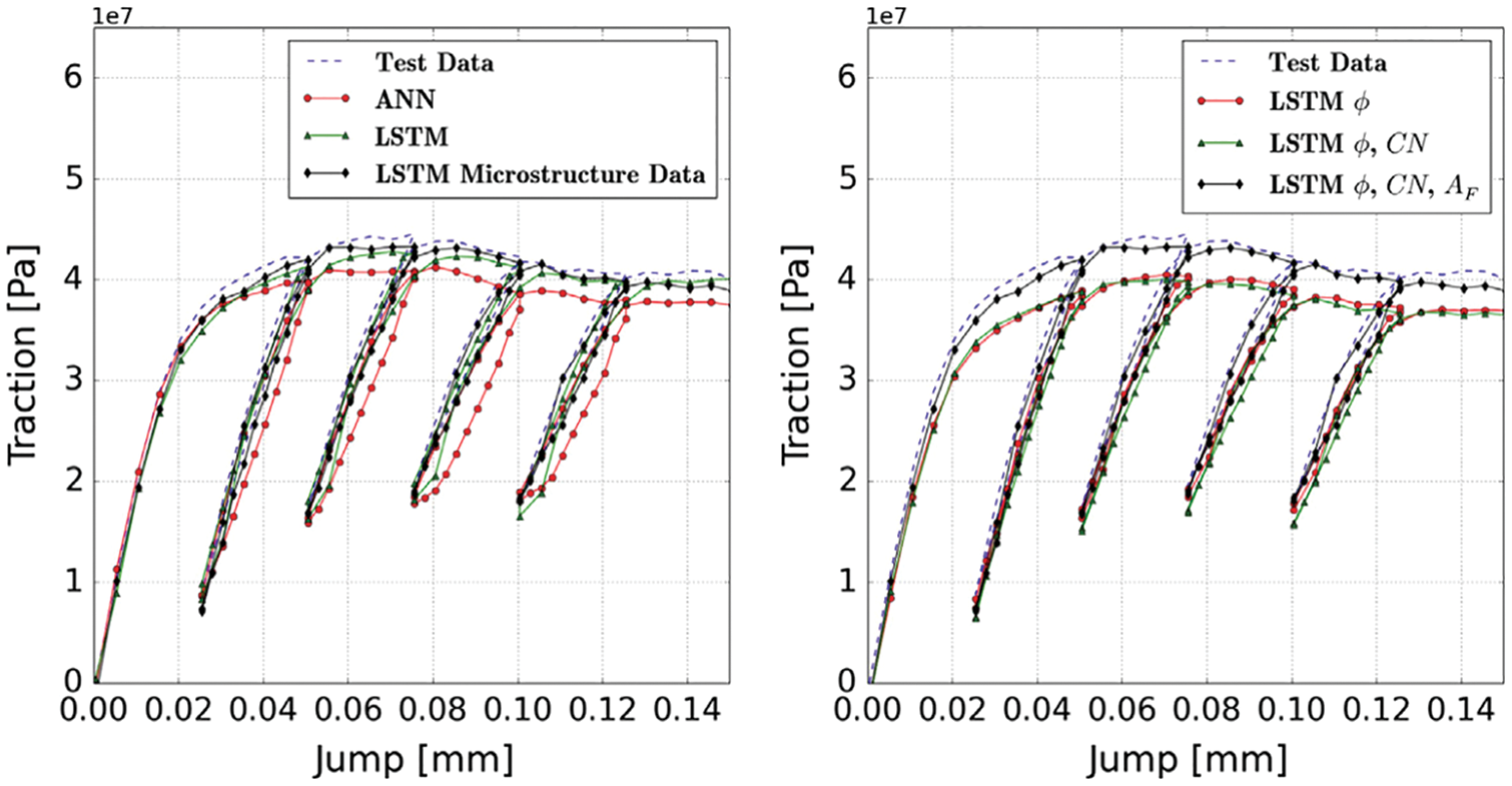
Figure 17: Network with LSTM and microstructure data (porosity
where
where
In a Galerkin-Project (GP) approach to reduced-order model, a small subset of dominant modes form a basis onto which high-dimensional differential equations are projected to obtain a set of lower-dimensional differential equations for cost-efficient computational analysis.
Instead of using GP, RNNs (Recurrent Neural Networks) were used in [26] to predict the evolution of fluid flows, specifically the coefficients of the dominant POD modes, rather than solving differential equations. For this purpose, their LSTM-ROM (Long Short-Term Memory - Reduced Order Model) approach combined concepts of ROM based on POD with deep-learning neural networks using either the original LSTM units, Figure 117 (left) [24], or the bidirectional LSTM (BiLSTM), Figure 117 (right) [104], the internal states of which were well-suited for the modeling of dynamical systems.
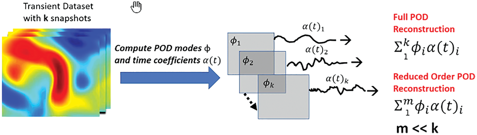
Figure 18: Reduced-order POD basis (Sections 2.3.3, 12.1). For each dataset (also Figure 116), which contained
To obtain training/testing data, which were crucial to train/test neural networks, the data from transient 3-D Direct Navier-Stokes (DNS) simulations of two physical problems, as provided by the Johns Hopkins turbulence database [105] were used [26]: (1) The Forced Isotropic Turbulence (ISO) and (2) The Magnetohydrodynamic Turbulence (MHD).
To generate training data for LSTM/BiLSTM networks, the 3-D turbulent fluid flow domain of each physical problem was decomposed into five equidistant 2-D planes (slices), with one additional equidistant 2-D plane served to generate testing data (Section 12, Figure 116, Remark 12.1). For the same subregion in each of those 2-D planes, POD was applied on the
(1) Multiple-network method: Use a RNN for each coefficient of the dominant POD modes
(2) Single-network method: Use a single RNN for all coefficients of the dominant POD modes
For both methods, variants with the original LSTM units or the BiLSTM units were implemented. Each of the employed RNN had a single hidden layer.
Demonstrative results for the prediction capabilities of both the original LSTM and the BiLSTM networks are illustrated in Figure 20. Contrary to the authors’ expectation, networks with the original LSTM units performed better than those using BiLSTM units in both physical problems of isotropic turbulence (ISO) (Figure 20a) and magnetohydrodyanmics (MHD) (Figure 20b) [26].
Details of the formulation in [26] are discussed in Section 12.
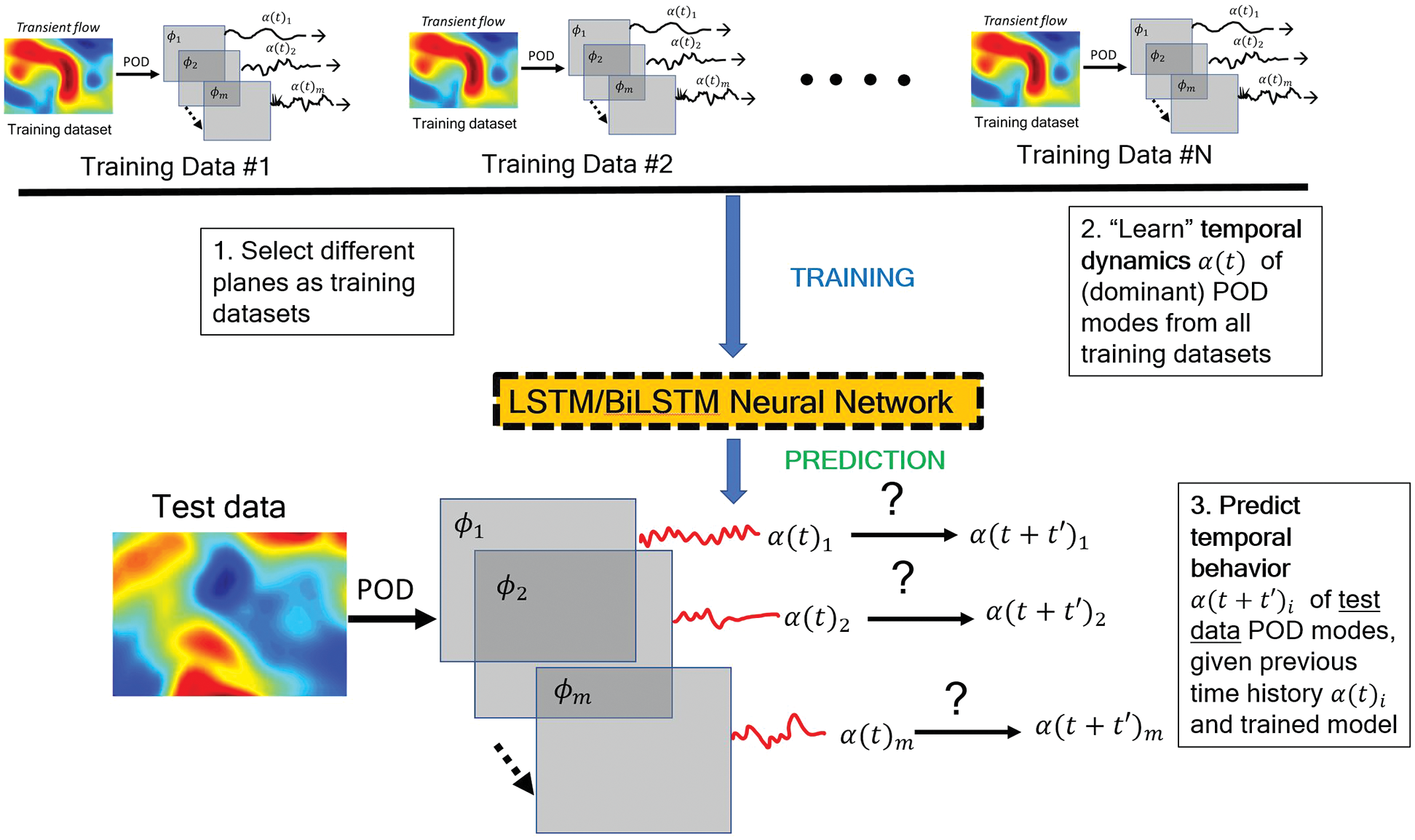
Figure 19: Deep-learning LSTM/BiLSTM Reduced Order Model (Sections 2.3.3, 12.2). See Figure 18 for POD reduced-order basis. The time-dependent coefficients
3 Computational mechanics, neuroscience, deep learning
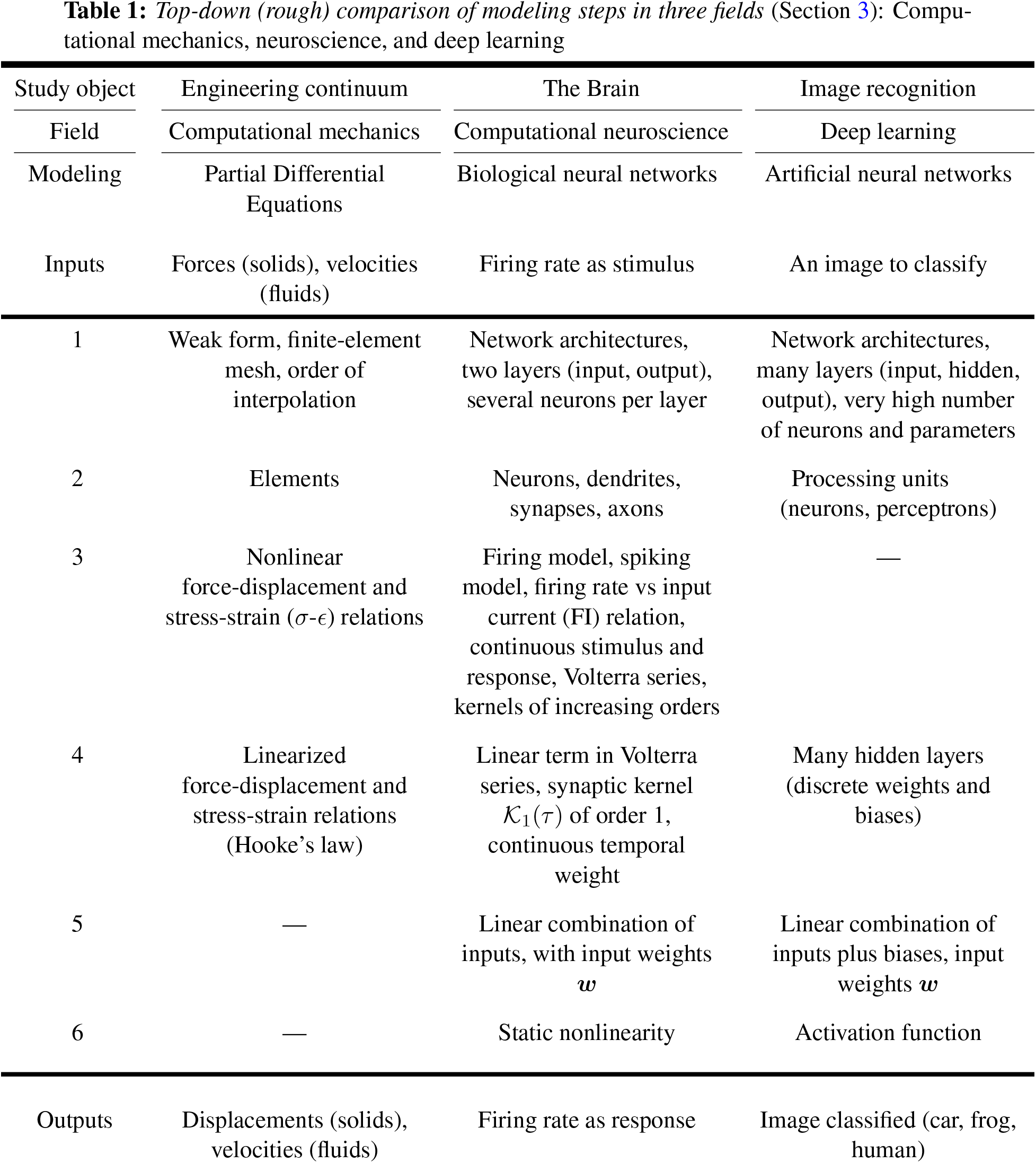
Table 1 below presents a rough comparison that shows the parallelism in the modeling steps in three fields: Computational mechanics, neuroscience, and deep learning, which heavily indebted to neuroscience until it reached more mature state, and then took on its own development.
We assume that readers are familiar with the concepts listed in the second column on “Computational mechanics”, and briefly explain some key concepts in the third column on “Neuroscience” to connect to the fourth column “Deep learning”, which is explained in detail in subsequent sections.
See Section 13.2 for more details on the theoretical foundation based on Volterra series for the spatial and temporal combinations of inputs, weights, and biases, widely used in artificial neural networks or multilayer perceptrons.
Neuron spiking response such as shown in Figure 21 can be modelled accurately using a model such as “Integrate-and-Fire”. The firing-rate response
where
where
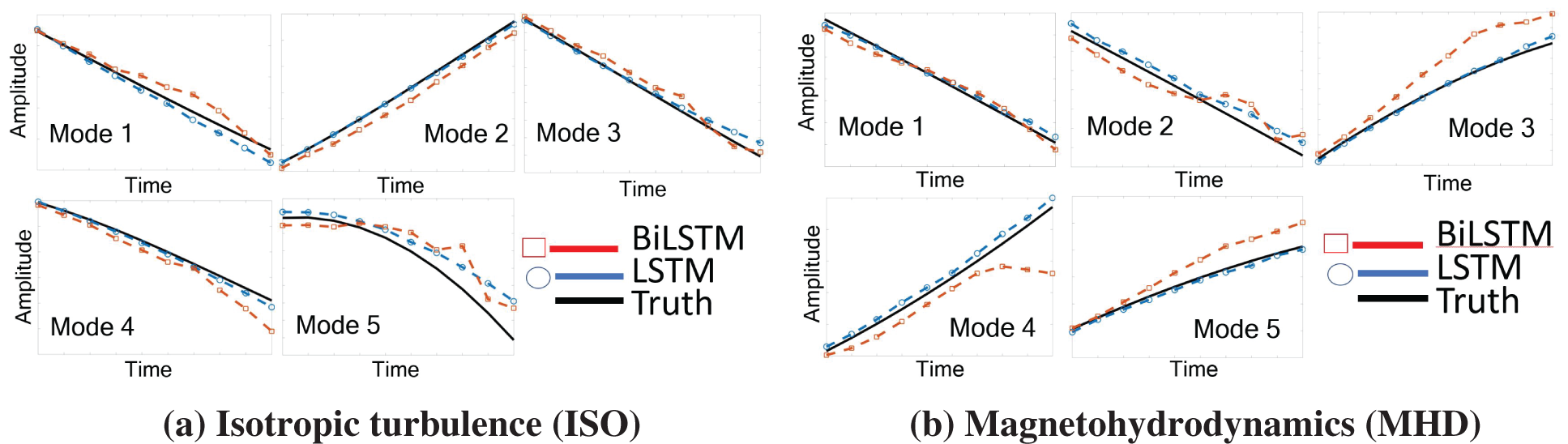
Figure 20: Prediction results and errors for LSTM/BiLSTM networks (Sections 2.3.3, 12.3). Coefficients αi(t), for i = 1, . . . , 5, of dominant POD modes. LSTM had smaller errors compared to BiLSTM for both physical problems (ISO and MHD).
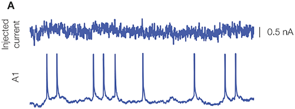
Figure 21: Biological neuron response to stimulus, experimental result (Section 3). An oscillating current was injected into the neuron (top), and neuron spiking response was recorded (below) [106], with permission from the authors and Frontiers Media SA. A spike, also called an action potential, is an electrical potential pulse across the cell membrane that lasts about 100 milivolts over 1 miliseconds. “Neurons represent and transmit information by firing sequences of spikes in various temporal patterns” [19], pp. 3-4.
It will be seen in Section 13.2.2 on “Dynamics, time dependence, Volterra series” that the convolution integral in Eq. (5) corresponds to the linear part of the Volterra series of nonlinear response of a biological neuron in terms of the stimulus, Eq. (497), which in turn provides the theoretical foundation for taking the linear combination of inputs, weights, and biases for an artificial neuron in a multilayer neural networks, as represented by Eq. (26).
The Integrate-and-Fire model for biological neuron provides a motivation for the use of the rectified linear units (ReLU) as activation function in multilayer neural networks (or perceptrons); see Figure 28.
Eq. (5) is also related to the exponential smoothing technique used in forecasting and applied to stochastic optimization methods to train multilayer neural networks; see Section 6.5.3 on “Forecasting time series, exponential smoothing”.
4 Statics, feedforward networks
We examine in detail the forward propagation in feedforward networks, in which the function mappings flow48 only one forward direction, from input to output.
There are two ways to present the concept of deep-learning neural networks: The top-down approach versus the bottom-up approach.
The top-down approach starts by giving up-front the mathematical big picture of what a neural network is, with the big-picture (high level) graphical representation, then gradually goes down to the detailed specifics of a processing unit (often referred to as an artificial neuron) and its low-level graphical representation. A definite advantage of this top-down approach is that readers new to the field immediately have the big picture in mind, before going down to the nitty-gritty details, and thus tend not to get lost. An excellent reference for the top-down approach is [78], and there are not many such references.
Specifically, for a multilayer feedforward network, by top-down, we mean starting from a general description in Eq. (18) and going down to the detailed construct of a neuron through a weighted sum with bias in Eq. (26) and then a nonlinear activation function in Eq. (35).
In terms of block diagrams, we begin our top-down descent from the big picture of the overall multilayer neural network with
The bottom-up approach typically starts with a biological neuron (see Figure 131 in Section 13.1 below), then introduces an artificial neuron that looks similar to the biological neuron (compare Figure 8 to Figure 131), with multiple inputs and a single output, which becomes an input to each of a multitude of other artificial neurons; see, e.g., [23] [21] [38] [20].49 Even though Figure 7, which preceded Figure 8 in [38], showed a network, but the information content is not the same as Figure 23.
Unfamiliar readers when looking at the graphical representation of an artificial neural network (see, e.g., Figure 7) could be misled in thinking in terms of electrical (or fluid-flow) networks, in which Kirchhoff’s law applies at the junction where the output is split into different directions to go toward other artificial neurons. The big picture is not clear at the outset, and could be confusing to readers new to the field, who would take some time to understand; see also Footnote 5. By contrast, Figure 23 clearly shows a multilevel function composition, assuming that first-time learners are familiar with this basic mathematical concept.
In mechanics and physics, tensors are intrinsic geometrical objects, which can be represented by infinitely many matrices of components, depending on the coordinate systems.50 vectors are tensors of order 1. For this reason, we do not use neither the name “vector” for a column matrix, nor the name “tensor” for an array with more than two indices.51 All arrays are matrices.
The matrix notation used here can follow either (1) the Matlab / Octave code syntax, or (2) the more compact component convention for tensors in mechanics.
Using Matlab / Octave code syntax, the inputs to a network (to be defined soon) are gathered in an
where the commas are separators for matrix elements in a row, and the semicolons are separators for rows. For matrix transpose, we stick to the standard notation using the superscript “
Using the component convention for tensors in mechanics,53 The coefficients of a
are arranged according to the following convention for the free indices
(1) In case both indices are subscripts, then the left subscript (index
(2) In case one index is a superscript, and the other index is a subscript, then the superscript (upper index
With this convention (lower index designates column index, while upper index designates row index), the coefficients of array
Instead of automatically associating any matrix variable such as
Consider the Jacobian matrix
where
where implicitly
are the spaces of column matrices, Then using the chain rule
where the summation convention on the repeated indices
Consider the scalar function
with
Now consider this particular scalar function below:57
Then the gradients of
4.3 Big picture, composition of concepts
A fully-connected feedforward network is a chain of successive applications of functions
or breaking Eq. (18) down, step by step, from inputs to outputs:59
Remark 4.1. The notation
The quantities associated with layer
are the predicted outputs from the previous layer
are the inputs to the subsequent layer
Remark 4.2. The output for layer
and can be used interchangeably. In the current Section 4 on “Static, feedforward networks”, the notation
The above chain in Eq. (18)—see also Eq. (23) and Figure 23—is referred to as “multiple levels of composition” that characterizes modern deep learning, which no longer attempts to mimic the working of the brain from the neuroscientific perspective.60 Besides, a complete understanding of how the brain functions is still far remote.61
4.3.1 Graphical representation, block diagrams
A function can be graphically represented as in Figure 22.

Figure 22: Function mapping, graphical representation (Section 4.3.1):
The multiple levels of compositions in Eq. (18) can then be represented by
revealing the structure of the feedforward network as a multilevel composition of functions (or chain-based network) in which the output

Figure 23: Feedforward network (Sections 4.3.1, 4.4.4): Multilevel composition in feedforward network with
Remark 4.3. Layer definitions, action layers, state layers. In Eq. (23) and in Figure 23, an action layer is defined by the action, i.e., the function
4.4 Network layer, detailed construct
4.4.1 Linear combination of inputs and biases
First, an affine transformation on the inputs (see Eq. (26)) is carried out, in which the coefficients of the inputs are called the weights, and the constants are called the biases. The output
The column matrix
is a linear combination of the inputs in
where the
and the
Both the weights and the biases are collectively known as the network parameters, defined in the following matrices for layer
For simplicity and convenience, the set of all parameters in the network is denoted by
Note that the set
Similar to the definition of the parameter matrix
with
The total number of parameters of a fully-connected feedforward network is then
But why using a linear (additive) combination (or superposition) of inputs with weights, plus biases, as expressed in Eq. (26) ? See Section 13.2.
An activation function
Without the activation function, the neural network is simply a linear regression, and cannot learn and perform complex tasks, such as image classification, language translation, guiding a driver-less car, etc. See Figure 32 for the block diagram of a one-layer network.
An example is a linear one-layer network, without activation function, being unable to represent the seemingly simple XOR (exclusive-or) function, which brought down the first wave of AI (cybernetics), and that is described in Section 4.5.
Rectified linear units (ReLU). Nowadays, for the choice of activation function
and depicted in Figure 24, for which the processing unit is called the rectified linear unit (ReLU),68 which was demonstrated to be superior to other activation functions in many problems.69 Therefore, in this section, we discuss in detail the rectified linear function, with careful explanation and motivation. It is important to note that ReLU is superior for large network size, and may have about the same, or less, accuracy than the older logistic sigmoid function for “very small” networks, while requiring less computational efforts.70
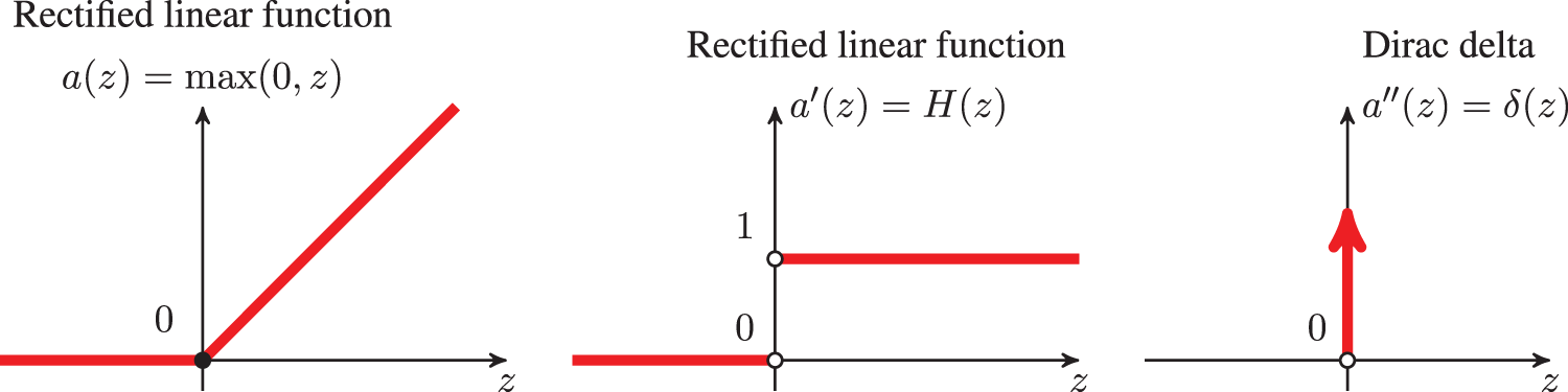
Figure 24: Activation function (Section 4.4.2): Rectified linear function and its derivatives. See also Section 5.3.3 and Figure 54 for Parametric ReLU that helped surpass human level performance in ImageNet competition for the first time in 2015, Figure 3 [61]. See also Figure 26 for a halfwave rectifier.
To transform an alternative current into a direct current, the first step is to rectify the alternative current by eliminating its negative parts, and thus The meaning of the adjective “rectified” in rectified linear unit (ReLU). Figure 25 shows the current-voltage relation for an ideal diode, for a resistance, which is in series with the diode, and for the resulting ReLU function that rectifies an alternative current as input into the halfwave rectifier circuit in Figure 26, resulting in a halfwave current as output.
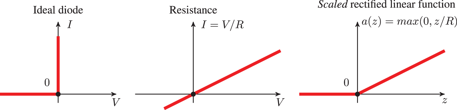
Figure 25: Current I versus voltage V (Section 4.4.2): Ideal diode, resistance, scaled rectified linear function as activation (transfer) function for the ideal diode and resistance in series. (Figure plotted with R = 2.) See also Figure 26 for a halfwave rectifier.
Mathematically, a periodic function remains periodic after passing through a (nonlinear) rectifier (active function):
where
Biological neurons encode and transmit information over long distance by generating (firing) electrical pulses called action potentials or spikes with a wide range of frequencies [19], p. 1; see Figure 27. “To reliably encode a wide range of signals, neurons need to achieve a broad range of firing frequencies and to move smoothly between low and high firing rates” [114]. From the neuroscientific standpoint, the rectified linear function could be motivated as an idealization of the “Type I” relation between the firing rate (F) of a biological neuron and the input current (I), called the FI curve. Figure 27 describes three types of FI curves, with Type I in the middle subfigure, where there is a continuous increase in the firing rate with increase in input current.
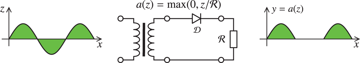
Figure 26: Halfwave rectifier circuit (Section 4.4.2), with a primary alternative current
The Shockley equation for a current
With the voltage across the resistance being
which is plotted in Figure 29. The rectified linear function could be seen from Figure 29 as a very rough approximation of the current-voltage relation in a halfwave rectifier circuit in Figure 26, in which a diode and a resistance are in series. In the Shockley model, the diode is leaky in the sense that there is a small amount of current flow when the polarity is reversed, unlike the case of an ideal diode or ReLU (Figure 24), and is better modeled by the Leaky ReLU activation function, in which there is a small positive (instead of just flat zero) slope for negative
Prior to the introduction of ReLU, which had been long widely used in neuroscience as activation function prior to 2011,71 the state-of-the-art for deep-learning activation function was the hyperbolic tangent (Figure 31), which performed better than the widely used, and much older, sigmoid function72 (Figure 30); see [113], in which it was reported that
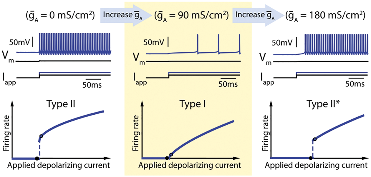
Figure 27: FI curves (Sections 4.4.2, 13.2.2). Firing rate frequency (F) versus applied depolarizing current (I), thus FI curves. Three types of FI curves. The time histories of voltage
“While logistic sigmoid neurons are more biologically plausible than hyperbolic tangent neurons, the latter work better for training multilayer neural networks. Rectifying neurons are an even better model of biological neurons and yield equal or better performance than hyperbolic tangent networks in spite of the hard non-linearity and non-differentiability at zero.”
The hard non-linearity of ReLU is localized at zero, but otherwise ReLU is a very simple function—identity map for positive argument, zero for negative argument—making it highly efficient for computation.
Also, due to errors in numerical computation, it is rare to hit exactly zero, where there is a hard non-linearity in ReLU:
“In the case of
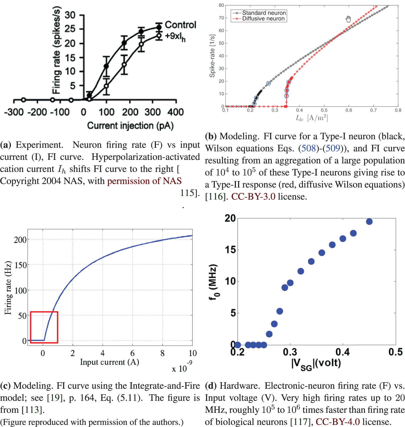
Figure 28: FI or FV curves (Sections 3, 4.4.2, 13.2.2). Neuron firing rate (F) versus input current (I) (FI curves, a,b,c) or voltage (V). The Integrate-and-Fire model in SubFigure (c) can be used to replace the sigmoid function to fit the experimental data points in SubFigure (a). The ReLU function in Figure 24 can be used to approximate the region of the FI curve just beyond the current or voltage thresholds, as indicated in the red rectangle in SubFigure (c). Despite the advanced mathematics employed to produce the Type-II FI curve of a large number of Type-I neurons, as shown in SubFigure (b), it is not clear whether a similar result would be obtained if the single neuron displays a behavior as in Figure 27, with transition from Type II to Type I to Type II* in a single neuron. See Section 13.2.2 on “Dynamic, time dependence, Volterra series” for more discussion on Wilson’s equations Eqs. (508)-(509) [118]. On the other hand for deep-learning networks, the above results are more than sufficient to motivate the use of ReLU, which has deep roots in neuroscience.
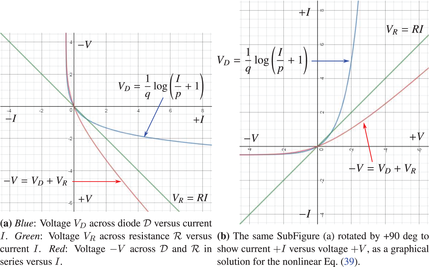
Figure 29: Halfwave rectifier (Sections 4.4.2, 5.3.2). Current I versus voltage V [red line in SubFigure (b)] in the halfwave rectifier circuit of Figure 26, for which the ReLU function in Figure 24 is a gross approximation. SubFigure (a) was plotted with p = 0.5, q = −1.2, R = 1. See also Figure 138 for the synaptic response of crayfish similar to the red line in SubFigure (b).
Thus, in addition to the ability to train deep networks, another advantage of using ReLU is the high efficiency in computing both the layer outputs and the gradients for use in optimizing the parameters (weights and biases) to lower cost or loss, i.e., training; see Section 6 on Training, and in particular Section 6.3 on Stochastic Gradient Descent.
The activation function ReLU approximates closer to how biological neurons work than other activation functions (e.g., logistic sigmoid, tanh, etc.), as it was established through experiments some sixty years ago, and have been used in neuroscience long (at least ten years) before being adopted in deep learning in 2011. Its use in deep learning is a clear influence from neuroscience; see Section 13.3 on the history of activation functions, and Section 13.3.2 on the history of the rectified linear function.
Deep-learning networks using ReLU mimic biological neural networks in the brain through a trade-off between two competing properties [113]:
(1) Sparsity. Only 1% to 4% of brain neurons are active at any one point in time. Sparsity saves brain energy. In deep networks, “rectifying non-linearity gives rise to real zeros of activations and thus truly sparse representations.” Sparsity provides representation robustness in that the non-zero features73 would have small changes for small changes of the data.
(2) Distributivity. Each feature of the data is represented distributively by many inputs, and each input is involved in distributively representing many features. Distributed representation is a key concept dated since the revival of connectionism with [119] [120] and others; see Section 13.2.1.
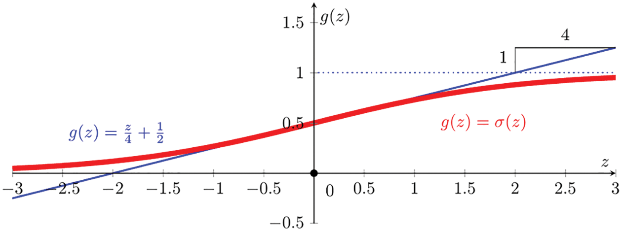
Figure 30: Logistic sigmoid function (Sections 4.4.2, 5.1.3, 5.3.1, 13.3.3):
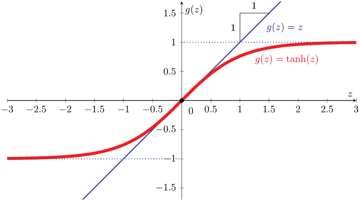
Figure 31: Hyperbolic tangent function (Section 4.4.2):
4.4.3 Graphical representation, block diagrams
The block diagram for a one-layer network is given in Figure 32, with more details in terms of the number of inputs and of outputs given in Figure 33.
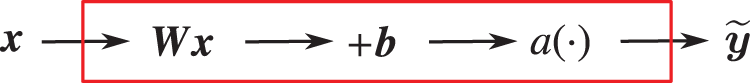
Figure 32: One-layer network (Section 4.4.3) representing the relation between the predicted output
For a multilayer neural network with
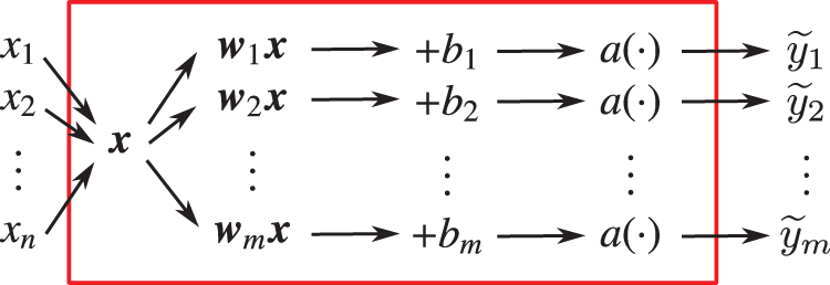
Figure 33: One-layer network (Section 4.4.3) in Figure 32: Lower level details, with

Figure 34: Input-to-output mapping (Sections 4.4.3, 4.4.4): Layer
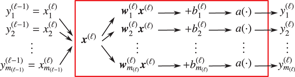
Figure 35: Low-level details of layer
And finally, we now complete our top-down descent from the big picture of the overall multilayer neural network with
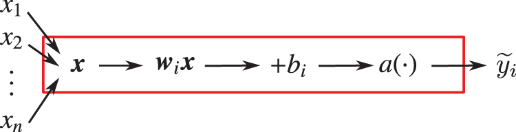
Figure 36: Artificial neuron (Sections 2.3.1, 4.4.4, 13.1), row
4.5 Representing XOR function with two-layer network
The XOR (exclusive-or) function played an important role in bringing down the first wave of AI, known as the cybernetics wave ([78], p. 14) since it was shown in [121] that Rosenblatt’s perceptron (1958 [119], 1962 [120] [2]) could not represent the XOR function, defined in Table 2:
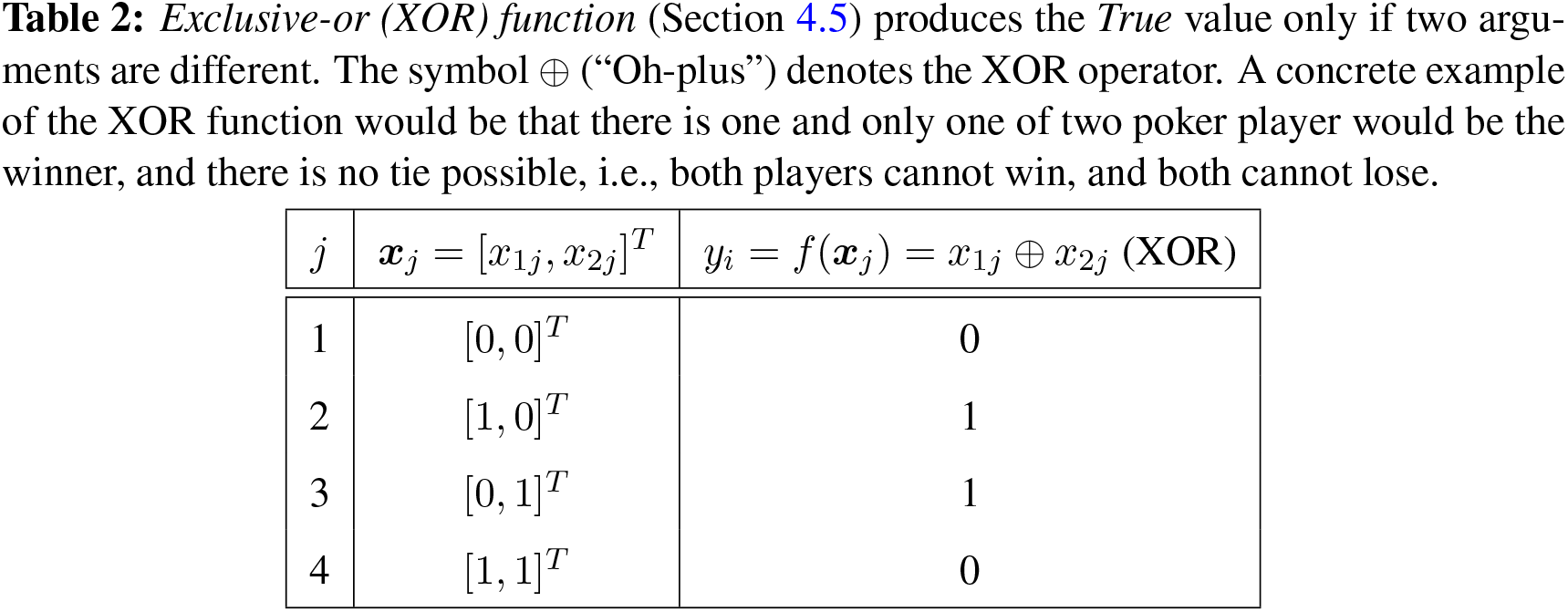
The dataset or design matrix74
An approximation (or prediction) for the XOR function
We begin with a one-layer network to show that it cannot represent the XOR function,75 then move on to a two-layer network, which can.
Consider the following one-layer network,76 in which the output
with the following matrices
since it is written in [78], p. 14:
“Model based on the
First-time learners, who have not seen the definition of Rosenblatt’s (1958) perceptron [119], could confuse Eq. (43) as the perceptron—which was not a linear model, but more importantly the Rosenblatt perceptron was a network with many neurons77—because Eq. (43) is only a linear unit (a single neuron), and does not have an (nonlinear) activation function. A neuron in the Rosenblatt perceptron is Eq. (489) in Section 13.2, with the Heaviside (nonlinear step) function as activation function; see Figure 132.
Figure 37: Representing XOR function (Sections 4.5, 13.2). This one-layer network (which is not the Rosenblatt perceptron in Figure 132) cannot perform this task. For each input matrix
The MSE cost function in Eq. (42) becomes
Setting the gradient of the cost function in Eq. (46) to zero and solving the resulting equations, we obtain the weights and the bias:
from which the predicted output
and thus this one-layer network cannot represent the XOR function. Eqs. (48) are called the “normal” equations.78
The four points in Table 2 are not linearly separable, i.e., there is no straight line that separates these four points such that the value of the XOR function is zero for two points on one side of the line, and one for the two points on the other side of the line. One layer could not represent the XOR function, as shown above. Rosenblatt (1958) [119] wrote:
“It has, in fact, been widely conceded by psychologists that there is little point in trying to ‘disprove’ any of the major learning theories in use today, since by extension, or a change in parameters, they have all proved capable of adapting to any specific empirical data. In considering this approach, one is reminded of a remark attributed to Kistiakowsky, that ‘given seven parameters, I could fit an elephant.’ ”
So we now add a second layer, and thus more parameters in the hope to be able to represent the XOR function, as shown in Figure 38.79
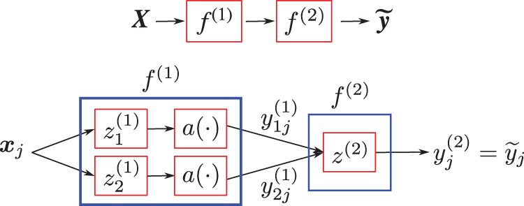
Figure 38: Representing XOR function (Sections 4.5). This two-layer network can perform this task. The four points in the design matrix
Layer (1): six parameters (4 weights, 2 biases), plus a (nonlinear) activation function. The purpose is to change coordinates to move the four input points of the XOR function into three points, such that the two points with XOR value equal 1 are coalesced into a single point, and such that these three points are aligned on a straight line. Since these three points remain not linearly separable, the activation function then moves these three points out of alignment, and thus linearly separable.
To map the two points
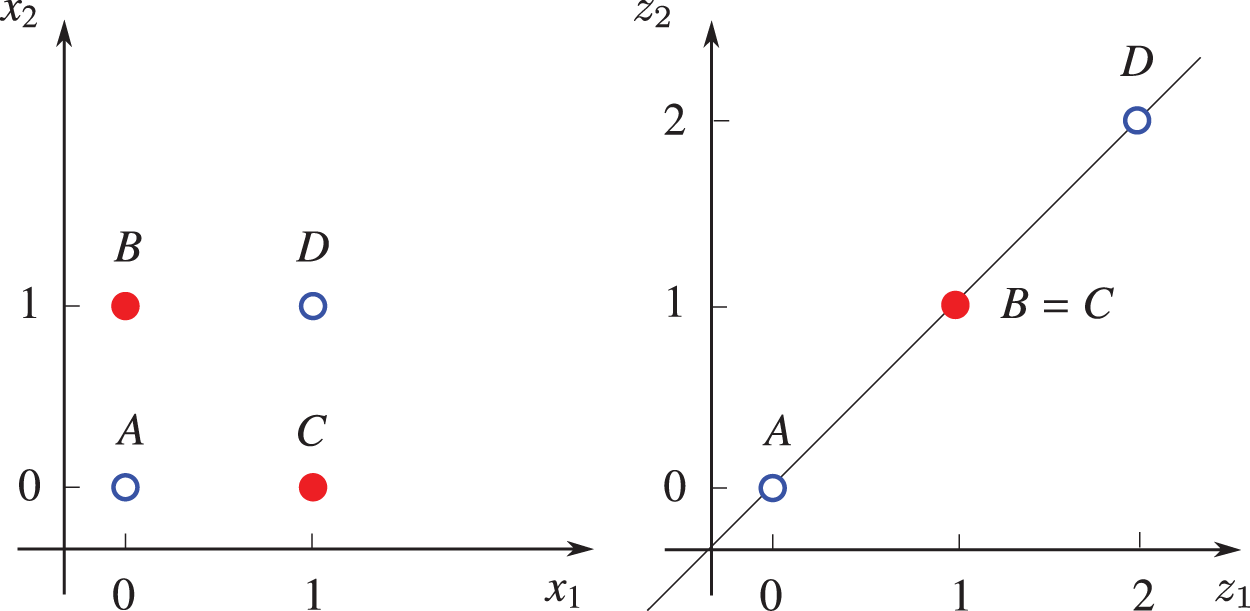
Figure 39: Two-layer network for XOR representation (Sections 4.5). Left: XOR function, with
For activation functions such as ReLu or Heaviside80 to have any effect, the above three points are next translated in the negative
and thus
For general activation function
Layer (2): three parameters (2 weights, 1 bias), no activation function. Eq. (59) for this layer is identical to Eq. (43) for the one-layer network above, with the output
with three distinct points in Eq. (57), because
We have three equations:
for which the exact analytical solution for the parameters
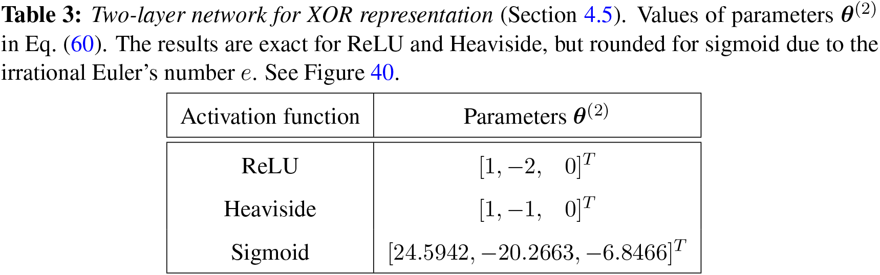
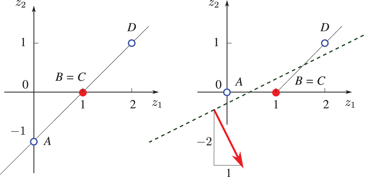
Figure 40: Two-layer network for XOR representation (Sections 4.5). Left: Images of points
We conjecture that any (nonlinear) function
Remark 4.4. Number of parameters. In 1953, Physicist Freeman Dyson (Princeton Institute of Advanced Study) once consulted with Nobel Laureate Enrico Fermi about a new mathematical model for a difficult physics problem that Dyson and his students had just developed. Fermi asked Dyson how many parameters they had. “Four”, Dyson replied. Fermi then gave his now famous comment “I remember my friend Johnny von Neumann used to say, with four parameters I can fit an elephant, and with five I can make him wiggle his trunk” [124].
But it was only more than sixty years later that physicists were able to plot an elephant in 2-D using a model with four complex numbers as parameters [125].
With nine parameters, the elephant can be made to walk (representing the XOR function), and with a billion parameters, it may even perform some acrobatic maneuver in 3-D; see Section 4.6 on depth of multilayer networks. ■
4.6 What is “deep” in “deep networks” ? Size, architecture
The concept of network depth turns out to be more complex than initially thought. While for a fully-connected feedforward neural network (in which all outputs of a layer are connected to a neuron in the following layer), depth could be considered as the number of layers, there is in general no consensus on the accepted definition of depth. It was stated in [78], p. 8, that:81
“There is no single correct value for the depth of an architecture,82 just as there is no single correct value for the length of a computer Program. Nor is there a consensus about how much depth a model requires to Qualify as “deep.” ”
For example, keeping the number of layers the same, then the “depth” of a sparsely-connected feedforward network (in which not all outputs of a layer are connected to a neuron in the following layer) should be smaller than the “depth” of a fully-connected feedforward network.
The lack of consensus on the boundary between “shallow” and “deep” networks is echoed in [12]:
“At which problem depth does Shallow Learning end, and Deep Learning begin? Discussions with DL experts have not yet yielded a conclusive response to this question. Instead of committing myself to a precise answer, let me just define for the purposes of this overview: problems of depth
Remark 4.5. Action depth, state depth. In view of Remark 4.3, which type of layer (action or state) were they talking about in the above quotation? We define here action depth as the number of action layers, and state depth as the number of state layers. The abstract network in Figure 23 has action depth
The review paper [13] was attributed in [38] for stating that “training neural networks with more than three hidden layers is called deep learning”, implying that a network is considered “deep” if its number of hidden (state) layers
An example of recognizing multidigit numbers in photographs of addresses, in which the test accuracy increased (or test error decreased) with increasing depth, is provided in [78], p. 196; see Figure 41.
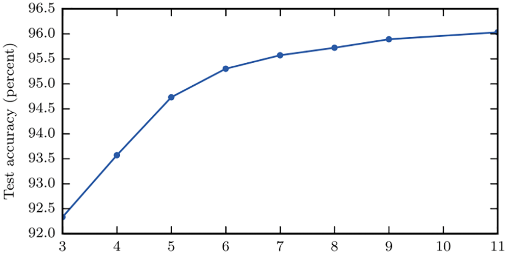
Figure 41: Test accuracy versus network depth (Section 4.6.1), showing that test accuracy for this example increases monotonically with the network depth (number of layers). [78], p. 196. (Figure reproduced with permission of the authors.)
But it is not clear where in [13] that it was actually said that a network is “deep” if the number of hidden (state) layers is greater than three. An example in image recognition having more than three layers was, however, given in [13] (emphases are ours):
“An image, for example, comes in the form of an array of pixel values, and the learned features in the first layer of representation typically represent the presence or absence of edges at particular orientations and locations in the image. The second layer typically detects motifs by spotting particular arrangements of edges, regardless of small variations in the edge positions. The third layer may assemble motifs into larger combinations that correspond to parts of familiar objects, and subsequent layers would detect objects as combinations of these parts.”
But the above was not a criterion for a network to be considered as “deep”. It was further noted on the number of the model parameters (weights and biases) and the size of the training dataset for a “typical deep-learning system” as follows [13] (emphases are ours):
“ In a typical deep-learning system, there may be hundreds of millions of these adjustable weights, and hundreds of millions of labelled examples with which to train the machine.”
See Remark 7.2 on recurrent neural networks (RNNs) as equivalent to “very deep feedforward networks”. Another example was also provided in [13]:
“Recent ConvNet [convolutional neural network, or CNN]83 architectures have 10 to 20 layers of ReLUs [rectified linear units], hundreds of millions of weights, and billions of connections between Units.”84
A neural network with 160 billion parameters was perhaps the largest in 2015 [126]:
“Digital Reasoning, a cognitive computing company based in Franklin, Tenn., recently announced that it has trained a neural network consisting of 160 billion parameters—more than 10 times larger than previous neural networks.
The Digital Reasoning neural network easily surpassed previous records held by Google’s 11.2-billion parameter system and Lawrence Livermore National Laboratory’s 15-billion parameter system.”
As mentioned above, for general network architectures (other than feedforward networks), not only that there is no consensus on the definition of depth, there is also no consensus on how much depth a network must have to qualify as being “deep”; see [78], p. 8, who offered the following intentionally vague definition:
“Deep learning can be safely regarded as the study of models that involve a greater amount of composition of either learned functions or learned concepts than traditional machine learning does.”
Figure 42 depicts the increase in the number of neurons in neural networks over time, from 1958 (Network 1 by Rosenblatt (1958) [119] in Figure 42 with one neuron, which was an error in [78], as discussed in Section 13.2) to 2014 (Network 20 GoogleNet with more than one million neurons), which was still far below the more than ten million biological neurons in a frog.
The architecture of a network is the number of layers (depth), the layer width (number of neurons per layer), and the connection among the neurons.85 We have seen the architecture of fully-connected feedforward neural networks above; see Figure 23 and Figure 35.
One example of an architecture different from that fully-connected feedforward networks is convolutional neural networks, which are based on the convolutional integral (see Eq. (497) in Section 13.2.2 on “Dynamic, time dependence, Volterra series”), and which had proven to be successful long before deep-learning networks:
“Convolutional networks were also some of the first neural networks to solve important commercial applications and remain at the forefront of commercial applications of deep learning today. By the end of the 1990s, this system deployed by NEC was reading over 10 percent of all the checks in the United States. Later, several OCR and handwriting recognition systems based on convolutional nets were deployed by Microsoft.” [78], p. 360.
“Fully-connected networks were believed not to work well. It may be that the primary barriers to the success of neural networks were psychological (practitioners did not expect neural networks to work, so they did not make a serious effort to use neural networks). Whatever the case, it is fortunate that convolutional networks performed well decades ago. In many ways, they carried the torch for the rest of deep learning and paved the way to the acceptance of neural networks in general.” [78], p. 361.
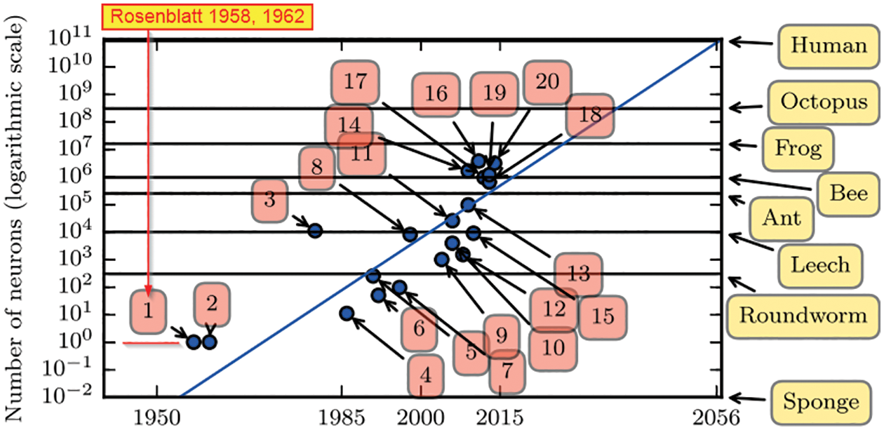
Figure 42: Increasing network size over time (Section 4.6.1, 13.2). All networks before 2015 had their number of neurons smaller than that of a frog at
Here, we present a more recent and successful network architecture different from the fully-connected feedforward network. Residual network was introduced in [127] to address the problem of vanishing gradient that plagued “very deep” networks with as few as 16 layers during training (see Section 5 on Backpropagation) and the problem of increased training error and test error with increased network depth as shown in Figure 43.
Remark 4.6. Training error, test (generalization) error. Using a set of data, called training data, to find the parameters that minimize the loss function (i.e., doing the training) provides the training error, which is the least square error between the predicted outputs and the training data. Then running the optimally trained model on a different set of data, which was not been used for the training, called test data, provides the test error, also known as generalization error. More details can be found in Section 6, and in [78], p. 107. ■
The basic building block of residual network is shown in Figure 44, and a full residual network in Figure 45. The rationale for residual networks was that, if the identity map were optimal, it would be easier for the optimization (training) process to drive the residual
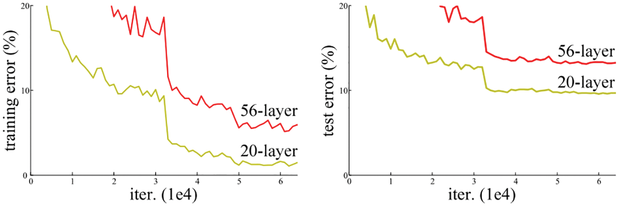
Figure 43: Training/test error vs. iterations, depth (Sections 4.6.2, 6). The training error and test error of deep fully-connected networks increased when the number of layers (depth) increased [127]. (Figure reproduced with permission of the authors.)
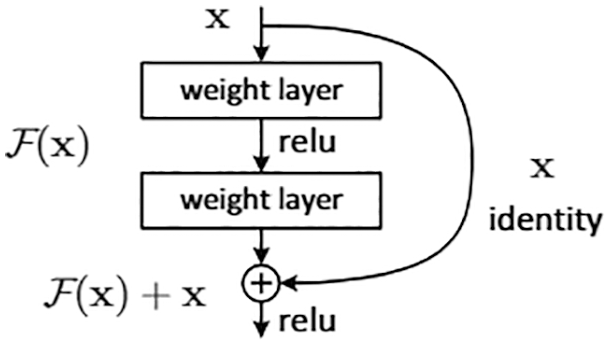
Figure 44: Residual network (Sections 4.6.2, 6), basic building block having two layers with the rectified linear activation function (ReLU), for which the input is
Remark 4.7. The identity map that jumps over a number of layers in the residual network building block in Figure 44 and in the full residual network in Figure 45 is based on a concept close to that for the path of the cell state
A deep residual network with more than 1,200 layers was proposed in [128]. A wide residual-network architecture that outperformed deep and thin networks was proposed in [129]: “For instance, [their] wide 16-layer deep network has the same accuracy as a 1000-layer thin deep network and a comparable number of parameters, although being several times faster to train.”
It is still not clear why some architecture worked well, while others did not:
“The design of hidden units is an extremely active area of research and does not yet have many definitive guiding theoretical principles.” [78], p. 186.
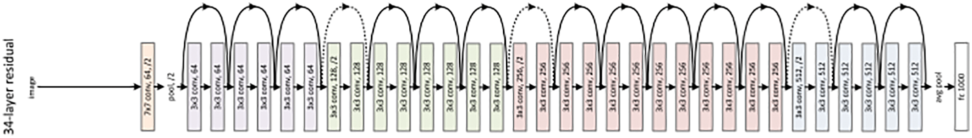
Figure 45: Full residual network (Sections 4.6.2, 6) with 34 layers, made up from 16 building blocks with two layers each (Figure 44), together with an input and an output layer. This residual network has a total of 3.6 billion floating-point operations (FLOPs with fused multiply-add operations), which could be considered as the network “computational depth” [127]. (Figure reproduced with permission of the authors.)
Backpropagation, sometimes abbreviated as “backprop”, was a child of whom many could claim to be the father, and is used to compute the gradient of the cost function with respect to the parameters (weights and biases); see Section 13.4.1 for a history of backpropagation. This gradient is then subsequently used in an optimization process, usually the Stochastic Gradient Descent method, to find the parameters that minimize the cost or loss function.
5.1 Cost (loss, error) function
Two types of cost function are discussed here: (1) the mean squared error (MSE), and (2) the maximum likelihood (probability cost).86
For a given input
The factor
While the components
where
5.1.2 Maximum likelihood (probability cost)
Many (if not most) modern networks employed a probability cost function based in the principle of maximum likelihood, which has the form of negative log-likelihood, describing the cross-entropy between the training data with probability distribution
where
The expectations of a function
Remark 5.1. Information content, Shannon entropy, maximum likelihood. The expression in Eq. (65)—with the minus sign and the log function—can be abstract to readers not familiar with the probability concept of maximum likelihood, which is related to the concepts of information content and Shannon entropy. First, an event
called the information content of
The product (chain) rule of conditional probabilities consists of expressing a joint probability of several random variables
The logarithm of the products in Eq. (69) and Eq. (70) is the sum of the factor probabilities, and provides another reason to use the logarithm in the expression for information content in Eq. (68): Independent events have additive information. Concretely, the information content of two asteroids independently hitting the Earth should double that of one asteroid hitting the Earth.
The parameters
where
is called the Principle of Maximum Likelihood, in which the model parameters are optimized to maximize the likelihood to reproduce the empirical data.92 ■
Remark 5.2. Relation between Mean Squared Error and Maximum Likelihood. The MSE is a particular case of the Maximum Likelihood. Consider having
as in Eq. (66), predicting the mean of this normal distribution,93 then
with
Then summing Eq. (77) over all examples
and thus the minimizer
where the MSE cost function
Thus finding the minimizer of the maximum likelihood cost function in Eq. (65) is the same as finding the minimizer of the MSE in Eq. (62); see also [78], p. 130. ■
Remark 5.2 justifies the use of Mean Squared Error as a Maximum Likelihood estimator.94 For the purpose of this review paper, it is sufficient to use the MSE cost function in Eq. (42) to develop the backpropagation procedure.
5.1.3 Classification loss function
In classification tasks—such as used in [38], Section 10.2, and Footnote 265—a neural network is trained to predict which of
The output of the neural network is supposed to represent the probability
In case more than two categories occur in a classification problem, a neural network is trained to estimate the probability distribution over the discrete number (
For this purpose, the idea of exponentiation and normalization, which can be expressed as a change of variable in the logistic sigmoid function
and is generalized then to vector-valued outputs; see also Figure 46.
The softmax function converts the vector formed by a linear unit
and is a smoothed version of the max function [130], p. 198.96
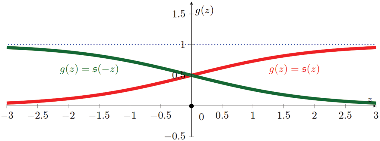
Figure 46: Sofmax function for two classes, logistic sigmoid (Section 5.1.3, 5.3.1):
Remark 5.3. Softmax function from Bayes’ theorem. For a classification with multiple classes
where the product rule was applied to the numerator of Eq. (85)
as in Eq. (83), and
Using a different definition, the softmax function (version 2) can be written as
which is the same as Eq. (84). ■
5.2 Gradient of cost function by backpropagation
The gradient of a cost function
Remark 5.4. We focus our attention on developing backpropagation for fully-connected networks, for which an explicit derivation was not provided in [78], but would help clarify the pseudocode.99 The approach in [78] was based on computational graph, which would not be familiar to first-time learners from computational mechanics, albeit more general in that it was applicable to networks with more general architecture, such as those with skipped connections, which require keeping track of parent and child processing units for constructing the path of backpropagation. See also Appendix 1 where the backprop Algorithm 1 below is rewritten in a different form to explain the equivalent Algorithm 6.4 in [78], p. 206. ■
It is convenient to recall here some equations developed earlier (keeping the same equation numbers) for the computation of the gradient
• Cost function
• Inputs
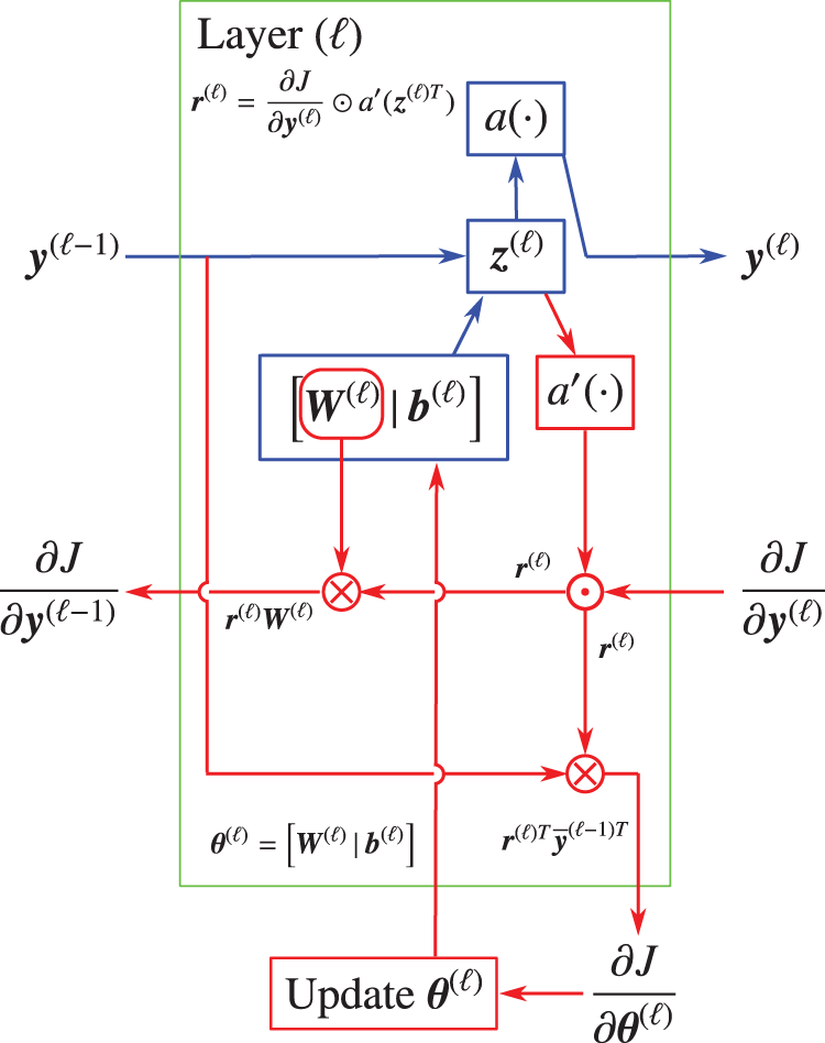
Figure 47: Backpropagation building block, typical layer
• Weighted sum of inputs and biases
• Network parameters
• Expanded layer outputs
• Activation function
The gradient of the cost function
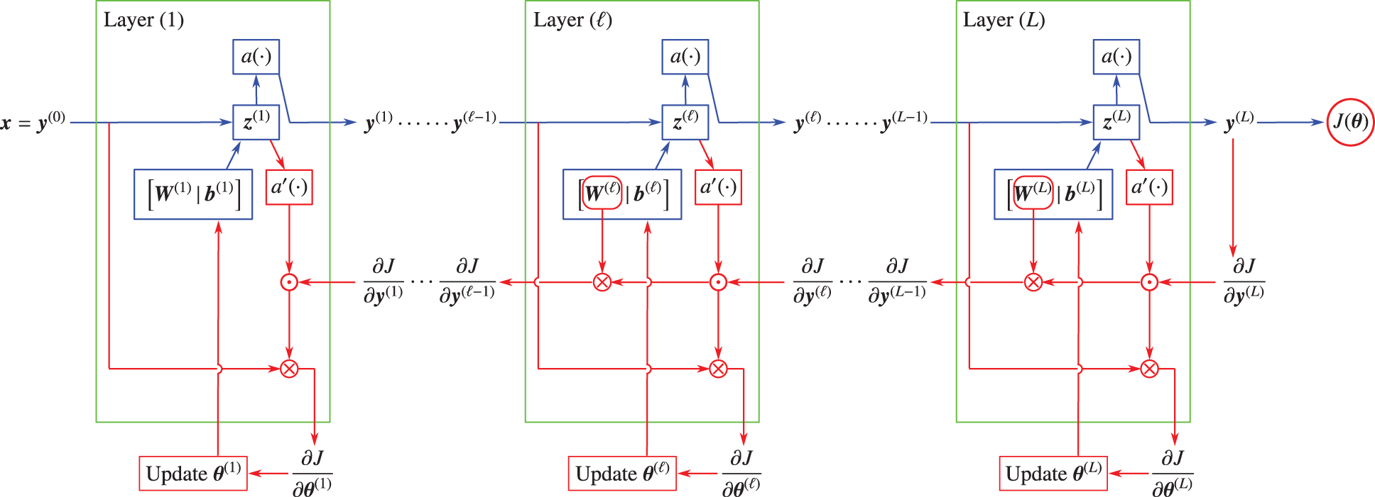
Figure 48: Backpropagation in fully-connected network (Section 5.2, 5.3, Algorithm 1, Appendix 1). Starting from the predicted output
The above equations are valid for the last layer
Using Eq. (93) in Eq. (91) leads to the expressions for the gradient, both in component form (left) and in matrix form (right):
where
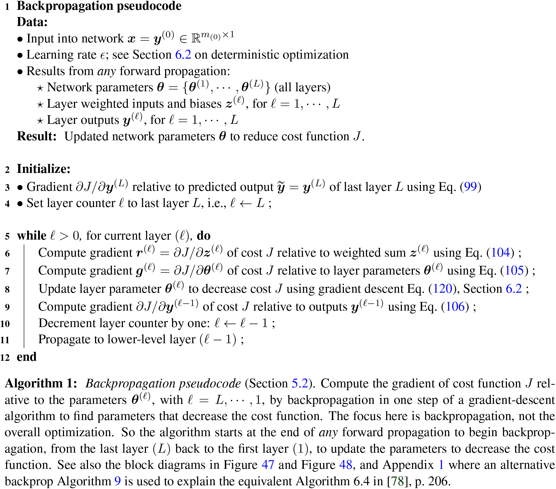
and
which then agrees with the matrix dimension in the first expression for
with
Comparing Eq. (101) and Eq. (98), when backpropagation reaches layer
is only needed to be computed once for use to compute both the gradient of the cost
and the gradient of the cost
The block diagram for backpropagation at layer
5.3 Vanishing and exploding gradients
To demonstrate the vanishing gradient problem, a network is used in [21], having an input layer containing 784 neurons, corresponding to the
We note immediately that the vanishing / exploding gradient problem can be resolved using the rectified linear function (ReLu, Figure 24) as active function in combination with “normalized initialization”100 and “intermediate normalization layers”, which are mentioned in [127], and which we will not discuss here.
The speed of learning of a hidden layer
The speed of learning in each of the four layers as a function of the number of epochs101 of training drops down quickly after less than 50 training epochs, then plateaued out, as depicted in Figure 49, where the speed of learning of layer (1) was 100 times less than that of layer (4) after 400 training epochs.
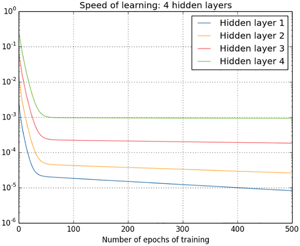
Figure 49: Vanishing gradient problem (Section 5.3). Speed of learning of earlier layers is much slower than that of later layers. Here, after 400 epochs of training, the speed of learning of Layer (1) at
To understand the reason for the quick and significant decrease in the speed of learning, consider a network with four layers, having one scalar input

Figure 50: Neural network with four layers (Section 5.3), one neuron per layer, scalar input
The neuron in layer
As an example of computing the gradient, the derivative of the cost function
The back propagation procedure to compute the gradient
Figure 51: Neural network with four layers in Figure 50 (Section 5.3). Detailed block diagram. Forward propagation (blue arrows) and backpropagation (red arrows). In the forward propagation wave, at each layer
Whether the gradient
In other mixed cases, the problem of vanishing or exploding gradient could be alleviated by the changing of the magnitude
Remark 5.5. While the vanishing gradient problem for multilayer networks (static case) may be alleviated by weights that vary from layer to layer (the mixed cases mentioned above), this problem is especially critical in the case of Recurrent Neural Networks, since the weights stay constant for all state numbers (or “time”) in a sequence of data. See Remark 7.3 on “short-term memory” in Section 7.2 on Long Short-Term Memory. In back-propagation through the states in a sequence of data, from the last state back to the first state, the same weight keeps being multiplied by itself. Hence, when a weight is less than 1, successive powers of its magnitude eventually decrease to zero when progressing back the first state. ■
5.3.1 Logistic sigmoid and hyperbolic tangent
The first derivatives of the sigmoid function and hyperbolic tangent function depicted in Figure 30 (also in Remark 5.3 on the softmax function and Figure 46) are given below:
and are less than 1 in magnitude (everywhere for the sigmoid function, and almost everywhere for the hyperbolic tangent tanh function), except at
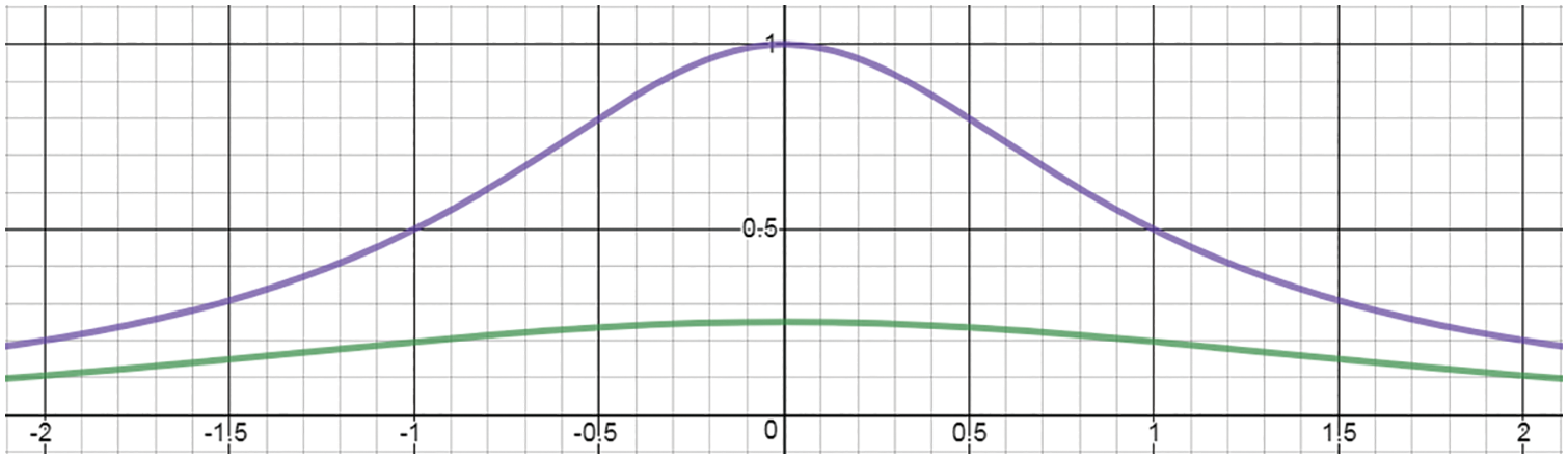
Figure 52: Sigmoid and hyperbolic tangent functions, derivative (Section 5.3.1). The derivative of sigmoid function (
The exploding gradient problem is opposite to the vanishing gradient problem, and occurs when the gradient has its magnitude increases in subsequent multiplications, particularly at a “cliff”, which is a sharp drop in the cost function in the parameter space.103 The gradient at the brink of a cliff (Figure 53) leads to large-magnitude gradients, which when multiplied with each other several times along the back propagation path would result in an exploding gradient problem.
5.3.2 Rectified linear function (ReLU)
The rectified linear function depicted in Figure 24 with its derivative (Heaviside function) equal to 1 for any input greater than zero, would resolve the vanishing-gradient problem, as it is written in [113]:
“For a given input only a subset of neurons are active. Computation is linear on this subset ... Because of this linearity, gradients flow well on the active paths of neurons (there is no gradient vanishing effect due to activation non-linearities of sigmoid or tanh units), and mathematical investigation is easier. Computations are also cheaper: there is no need for computing the exponential function in activations, and sparsity can be exploited.”
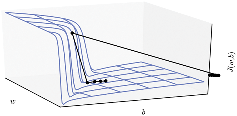
Figure 53: Cost-function cliff (Section 5.3.1). A cliff, or a sharp drop in the cost function. The parameter space is represented by a weight
A problem with ReLU was that some neurons were never activated, and called “dying” or “dead”, as described in [131]:
“However, ReLU units are at a potential disadvantage during optimization because the gradient is 0 whenever the unit is not active. This could lead to cases where a unit never activates as a gradient-based optimization algorithm will not adjust the weights of a unit that never activates initially. Further, like the vanishing gradients problem, we might expect learning to be slow when training ReL networks with constant 0 gradients.”
To remedy this “dying” or “dead” neuron problem, the Leaky ReLU, proposed in [131],104 had the expression already given previously in Eq. (40), and can be viewed as an approximation to the leaky diode in Figure 29. Both ReLU and Leaky ReLU have been known and used in neuroscience for years before being imported into artificial neural network; see Section 13 for a historical review.
5.3.3 Parametric rectified linear unit (PReLU)
Instead of arbitrarily fixing the slope
and thus the network adaptively learned the parameters to control the leaky part of the activation function. Using the Parametric ReLU in Eq.(115), a deep convolutional neural network (CNN) in [61] was able to surpass the level of human performance in image recognition for the first time in 2015; see Figure 3 on ImageNet competition results over the years.
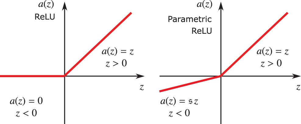
Figure 54: Rectified Linear Unit (ReLU, left) and Parametric ReLU (right) (Section 5.3.2), in which the slope
Figure 55: Cost-function landscape (Section 6). Residual network with 56 layers (ResNet-56) on the CIFAR-10 training set. Highly non-convex, with many local minima, and deep, narrow valleys [132]. The training error and test error for fully-connected network increased when the number of layers was increased from 20 to 56, Figure 43, motivating the introduction of residual network, Figure 44 and Figure 45, Section 4.6.2. (Figure reproduced with permission of the authors.)
6 Network training, optimization methods
For network training, i.e., to find the optimal network parameters
Figure 55 shows the highly non-convex landscape of the cost function of a residual network with 56 layers trained using the CIFAR-10 dataset (Canadian Institute For Advanced Research), a collection of images commonly used to train machine learning and computer vision algorithms, containing 60,000 32x32 color images in 10 different classes, representing airplanes, cars, birds, cats, deer, dogs, frogs, horses, ships, and trucks. Each class has 6,000 images.107
Deterministic optimization methods (Section 6.2) include first-order gradient method (Algorithm 2) and second-order quasi-Newton method (Algorithm 3), with line searches based on different rules, introduced by Goldstein, Armijo, and Wolfe.
Stochastic optimization methods (Section 6.3) include
• First-order stochastic gradient descent (SGD) methods (Algorithm 4), with add-on tricks such as momentum and accelerated gradient
• Adaptive learning-rate algorithms (Algorithm 5): Adam and variants such as AMSGrad, AdamW, etc. that are popular in the machine-learning community
• Criticism of adaptive methods and SGD resurgence with add-on tricks such as effective tuning and step-length decay (or annealing)
• Classical line search with stochasticity: SGD with Armijo line search (Algorithm 6), second-order Newton method with Armijo-like line search (Algorigthm 7)
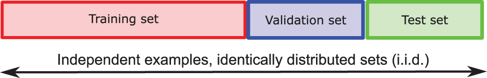
Figure 56: Training set, validation set, test set (Section 6.1). Partition of whole dataset. The examples are independent. The three subsets are identically distributed.
6.1 Training set, validation set, test set, stopping criteria
The classical (old) thinking—starting in 1992 with [133] and exemplified by Figures 57, 58, 59, 60 (a, left)—would surprise first-time learners that minimizing the training error is not optimal in machine learning. A reason is that training a neural network is different from using “pure optimization” since it is desired to decrease not only the error during training (called training error, and that’s pure optimization), but also the error committed by a trained network on inputs never seen before.108 Such error is called generalization error or test error. This classical thinking, known as the bias-variance trade-off, has been included in books since 2001 [134] (p. 194) and even repeated in 2016 [78] (p. 268). Models with lower number of parameters have higher bias and lower variance, whereas models with higher number of parameters have lower bias and higher variance; Figure 59.109
The modern thinking is exemplified by Figure 60 (b, right) and Figure 61, and does not contradict the intuitive notion that decreasing the training error to zero is indeed desirable, as overparameterizing networks beyond the interpolation threshold (zero training error) in modern practice generalizes well (small test error). In Figure 61, the test error continued to decrease significantly with increasing number of parameters
Such modern practice was the motivation for research into shallow networks with infinite width as a first step to understand how overparameterized networks worked so well; see Figure 148 and Section 14.2 “Lack of understanding on why deep learning worked.”
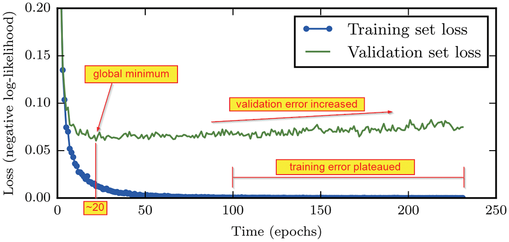
Figure 57: Training and validation learning curves—Classical viewpoint (Section 6.1), i.e., plots of training error and validation errors versus epoch number (time). While the training cost decreased continuously, the validation cost reaches a minimum around epoch 20, then started to gradually increase, forming an “asymmetric U-shaped curve.” Between epoch 100 and epoch 240, the training error was essentially flat, indicating convergence. Adapted from [78], p. 239. See Figure 60 (a, left), where the classical risk curve is the classical viewpoint, whereas the modern interpolation viewpoint is on the right subfigure (b). (Figure reproduced with permission of the authors.)
To develop a neural-network model, a dataset governed by the same probability distribution, such as the CIFAR-10 dataset mentioned above, can be typically divided into three non-overlapping subsets called training set, validation set, and test set. The validation set is also called the development set, a terminology used in [55], in which an effective method of step-length decay was proposed; see Section 6.3.4.
It was suggested in [135], p. 61, to use 50% of the dataset as training set, 25% as validation set, and 25% as test set. On the other hand, while a validation set with size about
Examples in the training set are fed into an optimizer to find the network parameter estimate
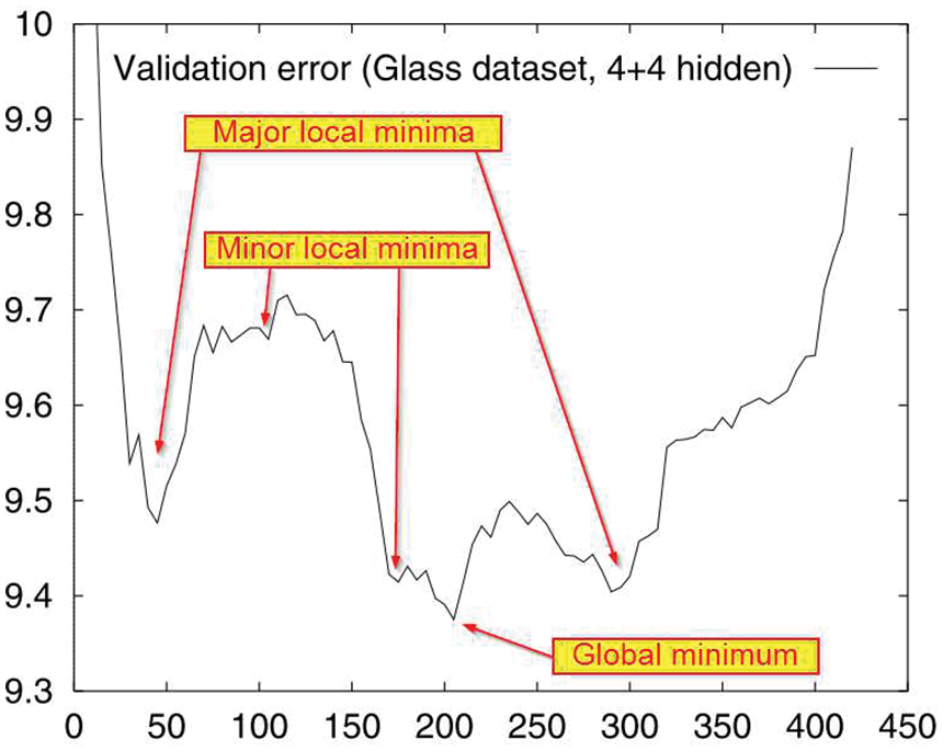
Figure 58: Validation learning curve (Section 6.1, Algorithm 4). Validation error vs epoch number. Some validation error could oscillate wildly around the mean, resulting in an “ugly reality”. The global minimum validation error corresponded to epoch number
Figure 57 shows the different behaviour of the training error versus that of the validation error. The validation error would decrease quickly initially, reaching a global minimum, then gradually increased, whereas the training error continued to decrease and plateaued out, indicating that the gradients got smaller and smaller, and there was not much decrease in the cost. From epoch 100 to epoch 240, the traning error was at about the same level, with litte noise. The validation error, on the other hand, had a lot of noise.
Because of the “asymmetric U-shaped curve” of the validation error, the thinking was that if the optimization process could stop early at the global mininum of the validation error, then the generalization (test) error, i.e., the value of cost function on the test set, would also be small, thus the name “early stopping”. The test set contains examples that have not been used to train the network, thus simulating inputs never seen before. The validation error could have oscillations with large amplitude around a mean curve, with many local minima; see Figure 58.
The difference between the test (generalization) error and the validation error is called the generalization gap, as shown in the bias-variance trade-off [133] Figure 59, which qualitatively delineates these errors versus model capacity, and conceptually explains the optimal model capacity as where the generalization gap equals the training error, or the generalization error is twice the training error.
Remark 6.1. Even the best machine learning generalization capability nowadays still cannot compete with the generalization ability of human babies; see Section 14.6 on “What’s new? Teaching machines to think like babies”. ■
Early-stopping criteria. One criterion is to first define the lowest validation error from epoch 1 up to the current epoch
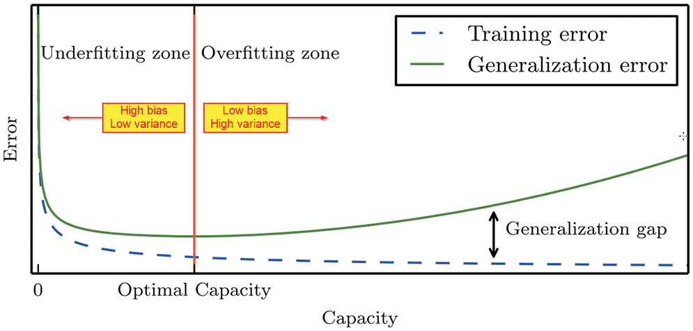
Figure 59: Bias-variance trade-off (Section 6.1). Training error (cost) and test error versus model capacity. Two ways to change the model capacity: (1) change the number of network parameters, (2) change the values of these parameters (weight decay). The generalization gap is the difference between the test (generalization) error and the training error. As the model capacity increases from underfit to overfit, the training error decreases, but the generalization gap increases, past the optimal capacity. Figure 72 gives examples of underfit, appropriately fit, overfit. See [78], p. 112. The above is the classical viewpoint, which is still prevalent [136]; see Figure 60 for the modern viewpoint, in which overfitting with high capacity model generalizes well (small test error) in practice. (Figure reproduced with permission of the authors.)
then define the generalization loss (in percentage) at epoch
[135] then defined the “first class of stopping criteria” as follows: Stop the optimization on the training set when the generalization loss exceeds a certain threshold
The issue is how to determine the generalization loss lower bound
Moreover, the above discussion is for the classical regime in Figure 60 (a). In the context of the modern interpolation regime in Figure 60 (b), early stopping means that the computation would cease as soon as the training error reaches “its lowest possible value (typically zero [beyond the interpolation threshold], unless two identical data points have two different labels)” [137]. See the green line in Figure 61.
Computational budget, learning curves. A simple method would be to set an epoch budget, i.e., the largest number of epochs for computation sufficiently large for the training error to go down significantly, then monitor graphically both the training error (cost) and the validation error versus epoch number. These plots are called the learning curves; see Figure 57, for which an epoch budget of 240 was used. Select the global minimum of the validation learning curve, with epoch number
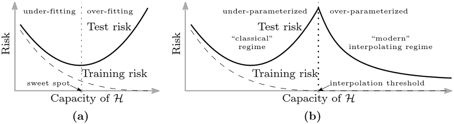
Figure 60: Modern interpolation regime (Sections 6.1, 14.2). Beyond the interpolation threshold, the test error goes down as the model capacity (e.g., number of parameters) increases, describing the observation that networks with high capacity beyond the interpolation threshold generalize well, even though overfit in training. Risk = error or cost. Capacity = number of parameters (but could also be increased by weight decay). Figures 57, 59 corresponds to the classical regime, i.e., old method (thinking) [136]. See Figure 61 for experimental evidence of the modern interpolation regime, and Figure 148 for a shallow network with infinite width. Permission of NAS.
Remark 6.2. Since it is important to monitor the validation error during training, a whole section is devoted in [78] (Section 8.1, p. 268) to expound on “How Learning Differs from Pure Optimization”. And also for this reason, it is not clear yet what global optimization algorithms such as in [138] could bring to network training, whereas the stochastic gradient descent (SGD) in Section 6.3.1 is quite efficient; see also Section 6.5.9 on criticism of adaptive methods. ■
Remark 6.3. Epoch budget, global iteration budget. For stochastic optimization algorithms—Sections 6.3, 6.5, 6.6, 6.7—the epoch counter is
Before presenting the stochastic gradient-descent (SGD) methods in Section 6.3, it is important to note that classical deterministic methods of optimization in Section 6.2 continue to be useful in the age of deep learning and SGD.
“One should not lose sight of the fact that [full] batch approaches possess some intrinsic advantages. First, the use full gradient information at each iterate opens the door for many deterministic gradient-based optimization methods that have been developed over the past decades, including not only the full gradient method, but also accelerated gradient, conjugate gradient, quasi-Newton, inexact Newton methods, and can benefit from parallelization.” [80], p. 237.
6.2 Deterministic optimization, full batch
Once the gradient
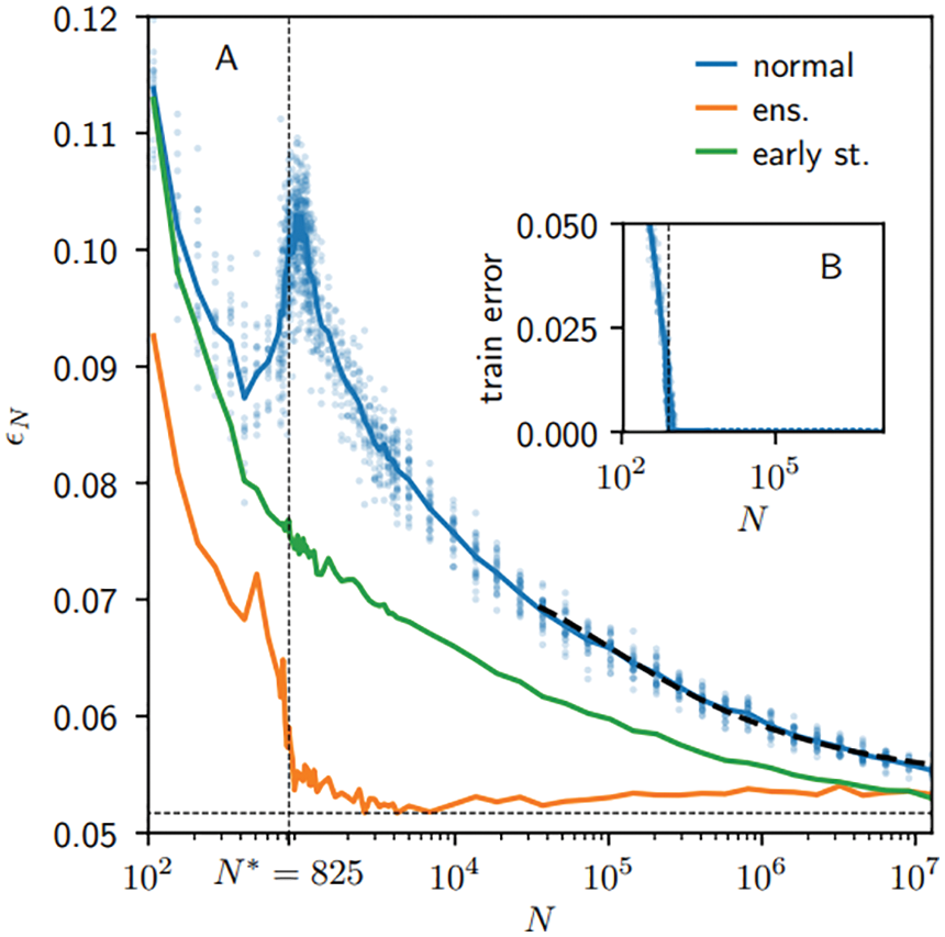
Figure 61: Empirical test error vs Number of paramesters (Sections 6.1, 14.2). Experiments using the MNIST handwritten digit database in [137] confirmed the modern interpolation regime in Figure 60 [136]. Blue: Average over 20 runs. Green: Early stopping. Orange: Ensemble average on
being the gradient direction, and
Otherwise, the update of the whole network parameter
where
“Neural network researchers have long realized that the learning rate is reliably one of the most difficult to set hyperparameters because it significantly affects model performance.” [78], p. 298.
In fact, it is well known in the field of optimization, where the learning rate is often mnemonically denoted by
“We can choose
Choosing an arbitrarily small
Remark 6.4. Line search in deep-learning training. Line search methods are not only important for use in deterministic optimization with full batch of examples,117 but also in stochastic optimization (see Section 6.3) with random mini-batches of examples [80]. The difficulty of using stochastic gradient coming from random mini-batches is the presence of noise or “discontinuities”118 in the cost function and in the gradient. Recent stochastic optimization methods—such as the sub-sampled Hessian-free Newton method reviewed in [80], the probabilisitic line search in [143], the first-order stochastic Armijo line search in [144], the second-order sub-sampling line search method in [145], quasi-Newton method with probabilitic line search in [146], etc.—where line search forms a key subprocedure, are designed to address or circumvent the noisy gradient problem. For this reason, claims that line search methods have “fallen out of favor”119 would be misleading, as they may encourage students not to learn the classics. A classic never dies; it just re-emerges in a different form with additional developments to tackle new problems. ■
In view of Remark 6.4, a goal of this section is to develop a feel for some classical deterministic line search methods for readers not familiar with these concepts to prepare for reading extensions of these methods to stochastic line search methods.
Find a positive step length
is negative, i.e., the descent direction
The minimization problem in Eq. (122) can be implemented using the Golden section search (or infinite Fibonacci search) for unimodal functions.121 For more general non-convex cost functions, a minimizing step length may be non-existent, or difficult to compute exactly.122 In addition, a line search for a minimizing step length is only an auxilliary step in an overall optimization algorithm. It is therefore sufficient to find an approximate step length satisfying some decrease conditions to ensure convergence to a local minimum, while keeping the step length from being too small that would hinder a reasonable advance toward such local minimum. For these reasons, inexact line search methods (rules) were introduced, first in [150], followed by [151], then [152] and [153]. In view of Remark 6.4 and Footnote 119, as we present these deterministic line-search rules, we will also immediately recall, where applicable, the recent references that generalize these rules by adding stochasticity for use as a subprocedure (inner loop) for the stochastic gradient-descent (SGD) algorithm.
6.2.2 Inexact line-search, Goldstein’s rule
The method is inexact since the search for an acceptable step length would stop before a minimum is reached, once the rule is satisfied.123 For a fixed constant
where both the numerator and the denominator are negative, i.e.,
A reason could be that the sector bounded by the two lines
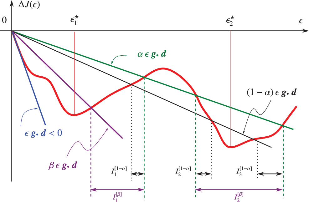
Figure 62: Inexact line search, Goldstein’s rule (Section 6.2.4). acceptable step lengths would be such that a decrease in the cost function
The search for an appropriate step length that satisfies Eq. (123) or Eq. (124) could be carried out by a subprocedure based on, e.g., the bisection method, as suggested in [139], p. 33. Goldstein’rule—also designated as Goldstein principle in the classic book [156], p. 256, since it ensured a decrease in the cost function—has been “used only occasionally” per Polak (1997) [149], p. 55, largely superceded by Armijo’s rule, and has not been generalized to add stochasticity. On the other hand, the idea behind Armijo’s rule is similar to Goldstein’s rule, but with a convenient subprocedure126 to find the appropriate step length.
6.2.3 Inexact line-search, Armijo’s rule
Apparently without the knowledge of [150], it was proposed in [151] the following highly popular Armijo step-length search,127 which recently forms the basis for stochastic line search for use in stochastic gradient-descent algorithm described in Section 6.3: Stochasticity was added to Armijo’s rule in [144], and the concept was extended to second-order line search [145]. Line search based on Armijo’s rule is also applied to quasi-Newton method for noisy functions in [158], and to exact and inexact subsampled Newton methods in [159].128
Armijo’s rule is stated as follows: For
where the decrease in the cost function along the descent direction
which is also known as the Armijo sufficient decrease condition, the first of the two Wolfe conditions presented below; see [152], [149], p. 55.130
Regarding the paramters
and proved a convergence theorem. In practice,
where
The pseudocode for deterministic gradient descent with Armijo line search is Algorithm 2, and the pseudocode for deterministic quasi-Newton / Newton with Armijo line search is Algorithm 3. When the Hessian
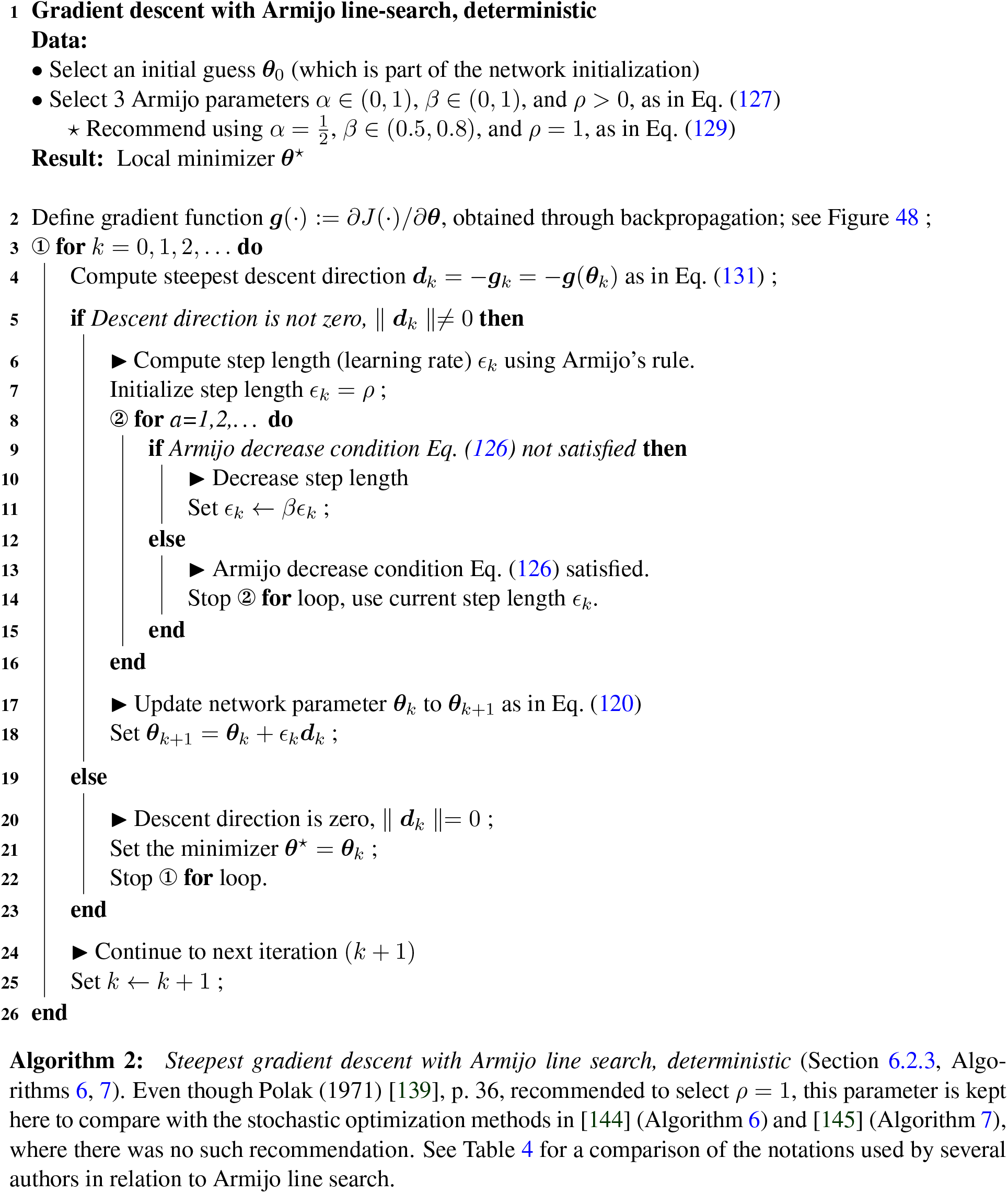
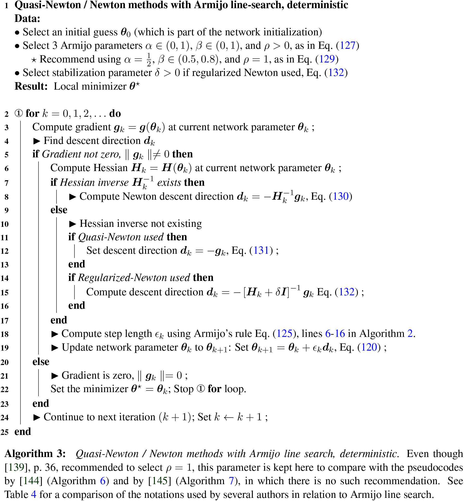
When the Hessian
and regularized Newton method uses a descent direction based on a regularized Hessian of the form:
where
6.2.4 Inexact line-search, Wolfe’s rule
The rule introduced in [152] and [153],136 sometimes called the Armijo-Goldstein-Wolfe’s rule (or conditions), particularly in [140] and [141],137 has been extended to add stochasticity [143],138 is stated as follows: For
The first Wolfe’s rule in Eq. (133) is the same as the Armijo’s rule in Eq. (126), which ensures that at the updated point
The second Wolfe’s rule in Eq. (134) is to ensure that at the updated point
For other variants of line search, we refer to [161].
6.3 Stochastic gradient-descent (1st-order) methods
To avoid confusion,139 we will use the terminology “full batch” (instead of just “batch”) when the entire training set is used for training. a minibatch is a small subset of the training set.
In fact, as we shall see, and as mentioned in Remark 6.4, classical optimization methods mentioned in Section 6.2 have been developed further to tackle new problems, such as noisy gradients, encountered in deep-learning training with random mini-batches. There is indeed much room for new research on learning rate since:
“The learning rate may be chosen by trial and error. This is more of an art than a science, and most guidance on this subject should be regarded with some skepticism.” [78], p. 287.
At the time of this writing, we are aware of two review papers on optimization algorithms for machine learning, and in particular deep learning, aiming particularly at experts in the field: [80], as mentioned above, and [162]. Our review complements these two review papers. We are aiming here at bringing first-time learners up to speed to benefit from, and even to hopefully enjoy, reading these and others related papers. To this end, we deliberately avoid the dense mathematical-programming language, not familiar to readers outside the field, as used in [80], while providing more details on algorithms that have proved important in deep learning than [162].
Listed below are the points that distinguish the present paper from other reviews. Similar to [78], both [80] and [162]:
• Only mentioned briefly in words the connection between SGD with momentum to mechanics without detailed explanation using the equation of motion of the “heavy ball”, a name not as accurate as the original name “small heavy sphere” by Polyak (1964) [3]. These references also did not explain how such motion help to accelerate convergence; see Section 6.3.2.
• Did not discuss recent practical add-on improvements to SGD such as step-length tuning (Section 6.3.3) and step-length decay (Section 6.3.4), as proposed in [55]. This information would be useful for first-time learners.
• Did not connect step-length decay to simulated annealing, and did not explain the reason for using the name “annealing”140 in deep learning by connecting to stochastic differential equation and physics; see Remark 6.9 in Section 6.3.5.
• Did not review an alternative to step-length decay by increasing minibatch size, which could be more efficient, as proposed in [164]; see Section 6.3.5.
• Did not point out that the exponential smoothing method (or running average) used in adaptive learning-rate algorithms dated since the 1950s in the field of forecasting. None of these references acknowledged the contributions made in [165] and [166], in which exponential smoothing from time series in forecasting was probably first brought to machine learning. See Section 6.5.3.
• Did not discuss recent adaptive learning-rate algorithms such as AdamW [56].141 These authors also did not discuss the criticism of adaptive methods in [55]; see Section 6.5.10.
• Did not discuss classical line-search rules—such as [150], [151],142 [152] (Sections 6.2.2, 6.2.3, 6.2.4)—that have been recently generalized to add stochasticity, e.g., [143], [144], [145]; see Sections 6.6, 6.7.
6.3.1 Standard SGD, minibatch, fixed learning-rate schedule
The stochastic gradient descent algorithm, originally introduced by Robbins & Monro (1951a) [167] (another classic) according to many sources,143 has been playing an important role in training deep-learning networks:
“Nearly all of deep learning is powered by one very important algorithm: stochastic gradient descent (SGD). Stochastic gradient descent is an extension of the gradient descent algorithm.” [78], p. 147.
Minibatch. The number
“The minibatch size
Generated as in Eq. (136), the random-index sets
Note that once the random index set
Unlike the iteration counter
Cost and gradient estimates. The cost-function estimate is the average of the cost functions, each of which is the cost function of an example
where we wrote the random index as
The pseudocode for the standard SGD146 is given in Algorithm 4. The epoch stopping criterion (line 1 in Algorithm 4) is usually determined by a computation “budget”, i.e., the maximum number of epochs allowed. For example, [145] set a budget of 1,600 epochs maximum in their numerical examples.
Problems and resurgence of SGD. There are several known problems with SGD:
“Despite the prevalent use of SGD, it has known challenges and inefficiencies. First, the direction may not represent a descent direction, and second, the method is sensitive to the step-size (learning rate) which is often poorly overestimated.” [144]
For the above reasons, it may not be appropriate to use the norm of the gradient estimate being small as stationarity condition, i.e., where the local minimizer or saddle point is located; see the discussion in [145] and stochastic Newton Algorithm 7 in Section 6.7.
Despite the above problems, SGD has been brought back to the forefront state-of-the-art algorithm to beat, surpassing the performance of adaptive methods, as confirmed by three recent papers: [55], [168], [56]; see Section 6.5.9 on criticism of adaptive methods.
Add-on tricks to improve SGD. The following tricks can be added onto the vanilla (standard) SGD to improve its performance; see also the pseudocode in Algorithm 4:
• Momentum and accelerated gradient: Improve (accelerate) convergence in narrow valleys, Section 6.3.2
• Initial-step-length tuning: Find effective initial step length
• Step-length decaying or annealing: Find an effective learning-rate schedule147 to decrease the step length
• Minibatch-size increase, keeping step length fixed, equivalent annealing, Section 6.3.5
• Weight decay, Section 6.3.6
6.3.2 Momentum and fast (accelerated) gradient
The standard update for gradient descent is Eq. (120) would be slow when encountering deep and narrow valley, as shown in Figure 63, and can be replaced by the general update with momentum as follows:
from which the following methods are obtained (line 10 in Algorithm 4):
• Standard SGD update Eq. (120) with
• SGD with classical momentum:
• SGD with fast (accelerated) gradient:149
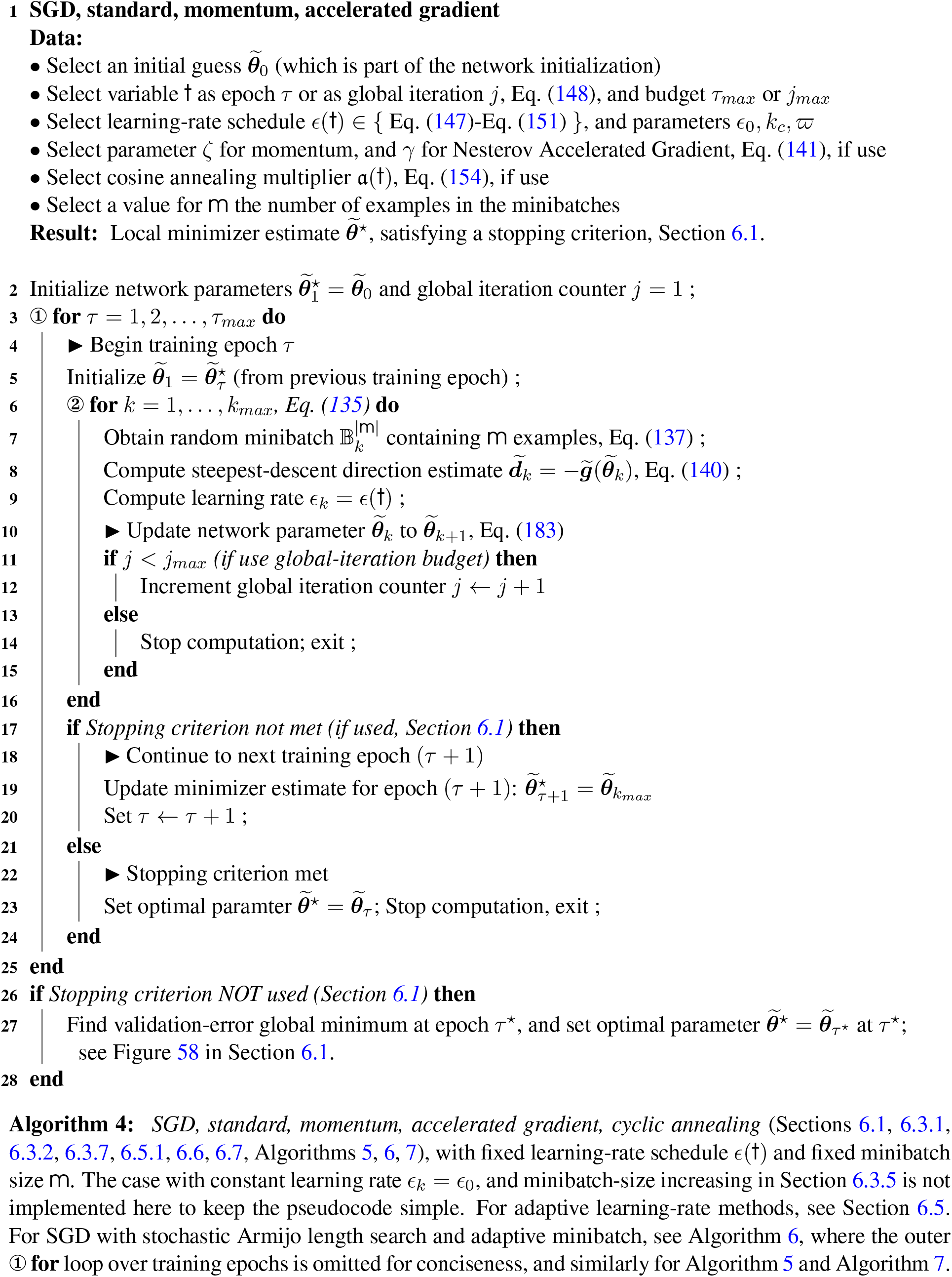
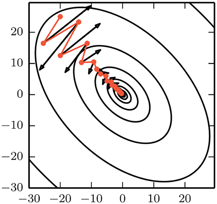
Figure 63: SGD with momentum, small heavy sphere Section 6.3.2. The descent direction (negative gradient, black arrows) bounces back and forth between the steep slopes of a deep and narrow valley. The small-heavy-sphere method, or SGD with momentum, follows a faster descent (red path) toward the bottom of the valley. See the cost-function landscape with deep valleys in Figure 55. Figure from [78], p. 289. (Figure reproduced with permission of the authors.)
The continuous counterpart of the parameter update Eq. (141) with classical momentum, i.e., when
which is the same as the update Eq. (141) with
Remark 6.5. The choice of the momentum parameter
Figure 68 from [170] shows the convergence of some adaptive learning-rate algorithms: AdaGrad, RMSProp, SGDNesterov (accelerated gradient), AdaDelta, Adam.
In their remarkable paper, the authors of [55] used a constant momentum parameter
See Figure 151 in Section 14.7 on “Lack of transparency and irreproducibility of results” in recent deep-learning papers. ■
For more insight into the update Eq. (143), consider the case of constant coefficients
i.e., without momentum for the first term. So the effective gradient is the sum of all gradients from the beginning
“Momentum is a simple method for increasing the speed of learning when the objective function contains long, narrow and fairly straight ravines with a gentle but consistent gradient along the floor of the ravine and much steeper gradients up the sides of the ravine. The momentum method simulates a heavy ball rolling down a surface. The ball builds up velocity along the floor of the ravine, but not across the ravine because the opposing gradients on opposite sides of the ravine cancel each other out over time.”
In recent years, Polyak (1964) [3] (English version)152 has often been cited for the classical momentum (“small heavy sphere”) method to accelerate the convergence in gradient descent, but not so before, e.g., the authors of [22] [175] [176] [177] [172] used the same method without citing [3]. Several books on optimization not related to neural networks, many of them well-known, also did not mention this method: [139] [178] [149] [157] [148] [179]. Both the original Russian version and the English translated version [3] (whose author’s name was spelled as “Poljak” before 1990) were cited in the book on neural networks [180], in which another neural-network book [171] was referred to for a discussion of the formulation.153
Remark 6.6. Small heavy sphere, or heavy point mass, is better name. Because the rotatory motion is not considered in Eq. (142), the name “small heavy sphere” given in [3] is more precise than the more colloquial name “heavy ball” often given to the SGD with classical momentum,154 since “small” implies that rotatory motion was neglected, and a “heavy ball” could be as big as a bowling ball155 for which rotatory motion cannot be neglected. For this reason, “heavy point mass” would be a precise alternative name. ■
Remark 6.7. For Nesterov’s fast (accelerated) gradient method, many references referred to [50].156 The authors of [78], p. 291, also referred to Nesterov’s 2004 monograph, which was mentioned in the Preface of, and the material of which was included in, [51]. For a special class of strongly convex functions,157 the step length can be kept constant, while the coefficients in Nesterov’s fast gradient method varied, to achieve optimal performance, [51], p. 92. “Unfortunately, in the stochastic gradient case, Nesterov momentum does not improve the rate of convergence” [78], p. 292. ■
6.3.3 Initial-step-length tuning
The initial step length
The following simple tuning method was proposed in [55]:
“To tune the step sizes, we evaluated a logarithmically-spaced grid of five step sizes. If the best performance was ever at one of the extremes of the grid, we would try new grid points so that the best performance was contained in the middle of the parameters. For example, if we initially tried step sizes 2, 1, 0.5, 0.25, and 0.125 and found that 2 was the best performing, we would have tried the step size 4 to see if performance was improved. If performance improved, we would have tried 8 and so on.”
The above logarithmically-spaced grid was given by
• SGD (Section 6.3.1): 2, 1, 0.5 (best), 0.25, 0.05, 0.01158
• SGD with momentum (Section 6.3.2): 2, 1, 0.5 (best), 0.25, 0.05, 0.01
• AdaGrad (Section 6.5): 0.1, 0.05, 0.01 (best, default), 0.0075, 0.005
• RMSProp (Section 6.5): 0.005, 0.001, 0.0005, 0.0003 (best), 0.0001
• Adam (Section 6.5): 0.005, 0.001 (default), 0.0005, 0.0003 (best), 0.0001, 0.00005
6.3.4 Step-length decay, annealing and cyclic annealing
In the update of the parameter
The following learning-rate scheduling, linear with respect to
where
with
Another step-length decay method proposed in [55] is to reduce the step length
Recall,
Cyclic annealing. In additional to decaying the step length
as an add-on to the parameter update for vanilla SGD Eq. (120), or
as an add-on to the parameter update for SGD with momentum and accelerated gradient Eq. (141). The cosine annealing factor can take the form [56]:
where
Figure 74 shows the effectiveness of cosine annealing in bringing down the cost rapidly in the early stage, but there is a diminishing return, as the cost reduction decreases with the number of annealing cycle. Up to a point, it is no longer as effective as SGD with weight decay in Section 6.3.6.
Convergence conditions. The sufficient conditions for convergence, for convex functions, are162
The inequality on the left of Eq. (155), i.e., the sum of the squared of the step lengths being finite, ensures that the step length would decay quickly to reach the minimum, but is valid only when the minibatch size is fixed. The equation on the right of Eq. (155) ensures convergence, no matter how far the initial guess was from the minimum [164].
In Section 6.3.5, the step-length decay is shown to be equivalent to minibatch-size increase and simulated annealing in the sense that there would be less fluctuation, and thus lower “temperature” (cooling) by analogy to the physics governed by the Langevin stochastic differential equation and its discrete version, which is analogous to the network parameter update.
6.3.5 Minibatch-size increase, fixed step length, equivalent annealing
The minibatch parameter update from Eq. (141), without momentum and accelerated gradient, which becomes Eq. (120), can be rewritten to introduce the error due to the use of the minibatch gradient estimate
where
To show that the gradient error has zero mean (average), based on the linearity of the expectation function
from Eqs. (135)-(137) on the definition of minibatches and Eqs. (139)-(140) on the definition of the cost and gradient estimates (without omitting the iteration counter
Or alternatively, the same result can be obtained with:
Next, the mean value of the “square” of the gradient error, i.e.,
where
Eq. (163) is the key relation to derive an expression for the square of the gradient error
where the iteration counter
Now assume the covariance matrix of any pair of single-example gradients
where
The authors of [164] introduced the following stochastic differential equation as a continuous counterpart of the discrete parameter update Eq. (156), as
where
where
The fluctuation factor
Remark 6.8. Fluctuation factor for large training set. For large
since their cost function was not an average, i.e., not divided by the minibatch size
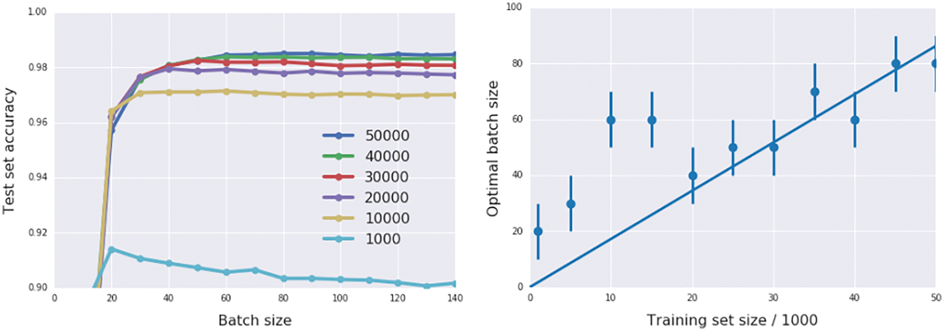
Figure 64 Optimal minibatch size vs. training-set size (Section 6.3.5). For a given trainingset size, the smallest minibatch size that achieves the highest accuracy is optimal. Left figure: The optimal mimibatch size was moving to the right with increasing training-set size M. Right figure: The optimal minibatch size in [186] is linearly proportional to the training-set size M for large training sets (i.e., M ← ∞), Eq. (173), but our fluctuation factor ℱ is independent of M when M ← ∞; see Remark 6.8. (Figure reproduced with permission of the authors.)
It was suggested in [164] to follow the same step-length decay schedules166
The results are shown in Figure 66, where it was shown that the number of updates decreased drastically with minibatch-size increase, allowing for significantly shortening the training wall-clock time.
Remark 6.9. Langevin stochastic differential equation, annealing. Because the fluctuation factor
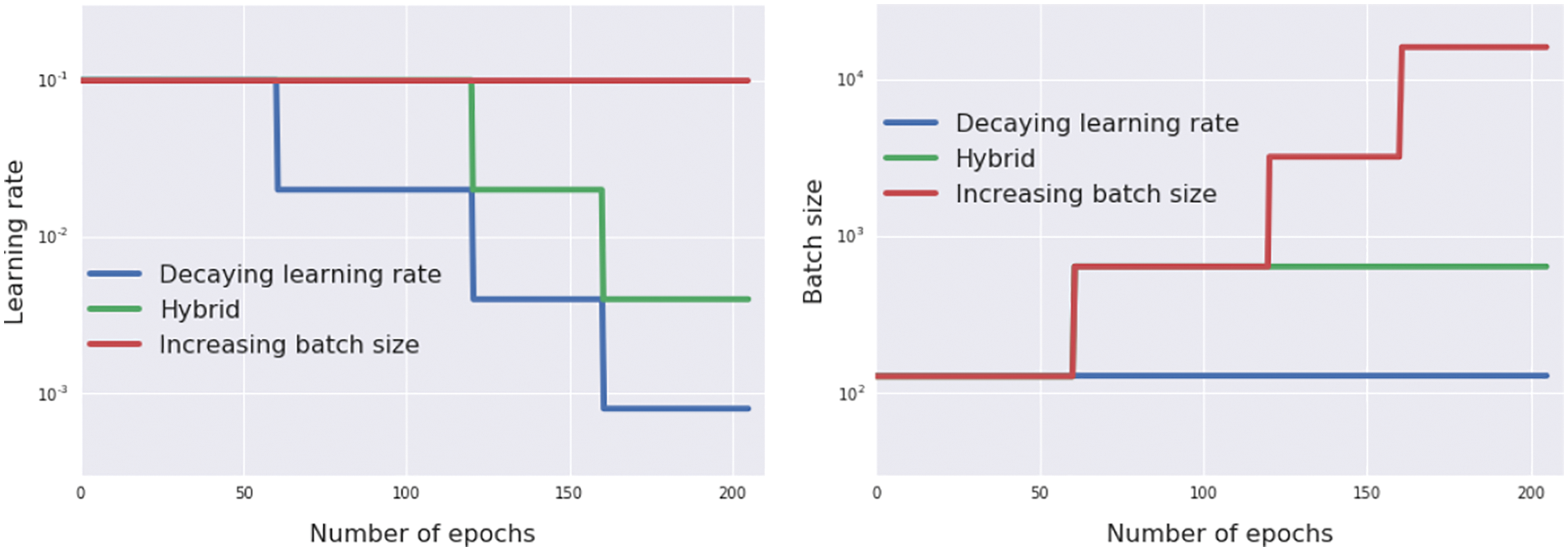
Figure 65: Minibatch-size increase vs. step-length decay, training schedules (Section 6.3.5). Left figure: Step length (learning rate) vs. number of epochs. Right figure: Minibatch size vs. number of epochs. Three learning-rate schedules167 were used for training: (1) The step length was decayed by a factor of 5, from an initial value of
Even though the authors of [164] referred to [187] for Eq. (169), the decomposition of the parameter update in [187]:
with the intriguing factor
where
The column matrix (or vector)
To obtain a differential equation, Eq. (175) can be rewritten as
which shows that the derivative of
The last term
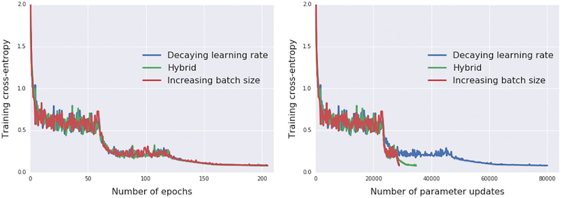
Figure 66: Minibatch-size increase, fewer parameter updates, faster comutation (Section 6.3.5). For each of the three training schedules in Figure 65, the same learning curve is plotted in terms of the number of epochs (left figure), and again in terms of the number of parameter updates (right figure), which shows the significant decrease in the number of parameter updates, and thus computational cost, for the training schedule with minibatch-size decrease. The blue curve ends at about 80,000 parameter updates for step-length decrease, whereas the red curve ends at about 29,000 parameter updates for minibatch-size decrease [164] (Figure reproduced with permission of the authors.)
where
where
The covariance of the noise
Eq. (178) cannot be directly integrated to obtain the velocity
where
Remark 6.10. Metaheuristics and nature-inspired optimization algorithms. There is a large class of nature-inspired optimization algorithms that implemented the general conceptual metaheuristics—such as neighborhood search, multi-start, hill climbing, accepting negative moves, etc.—and that include many well-known methods such as Evolutionary Algorithms (EAs), Artificial Bee Colony (ABC), Firefly Algorithm, etc. [190].
The most famous of these nature-inspired algorithms would be perhaps simulated annealing in [163], which is described in [191], p. 18, as being “inspired by the annealing process of metals. It is a trajectory-based search algorithm starting with an initial guess solution at a high temperature and gradually cooling down the system. A move or new solution is accepted if it is better; otherwise, it is accepted with a probability, which makes it possible for the system to escape any local optima”, i.e., the metaheuristic “accepting negative moves” mentioned in [190]. “It is then expected that if the system is cooled down slowly enough, the global optimal solution can be reached”, [191], p. 18; that’s step-length decay or minibatch-size increase, as mentioned above. See also Footnotes 140 and 168.
For applications of these nature-inspired algorithms, we cite the following works, without detailed review: [191] [192] [193] [194] [195] [196] [197] [198] [199]. ■
6.3.6 Weight decay, avoiding overfit
Reducing, or decaying, the network parameters
where
It was written in [201] that: “In the neural network community the two most common methods to avoid overfitting are early stopping and weight decay [175]. Early stopping has the advantage of being quick, since it shortens the training time, but the disadvantage of being poorly defined and not making full use of the available data. Weight decay, on the other hand, has the advantage of being well defined, but the disadvantage of being quite time consuming” (because of tuning). For examples of tuning the weight decay parameter
In the case of weight decay with cyclic annealing, both the step length
The effectiveness of SGD with weight decay, with and without cyclic annealing, is presented in Figure 74.
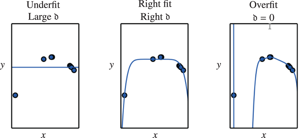
Figure 67: Weight decay (Section 6.3.6). Effects of magnitude of weight-decay parameter
6.3.7 Combining all add-on tricks
To have a general parameter-update equation that combines all of the above add-on improvement tricks, start with the parameter update with momentum and accelerated gradient Eq. (141)
and add the weight-decay term
which is included in Algorithm 4.
All optimization algorithms discussed above share a crucial step, which crucially affects the convergence of training, especially as neural networks become ‘deep’: The initialization of the network’s parameters
The Kaiming He initialization provides equally effective as simple means to overcome scaling issues observed when weights are randomly initialized using a normal distribution with fixed standard deviation. The key idea of the authors [127] is to have the same variance of weights for each of the network’s layers. As opposed to the Xavier initialization174, the nonlinearity of activation functions is accounted for. Consider the
where
where
is a measure of the “dispersion” of
As opposed to the variance, the standard deviation of some random variable
The elementary relation
Note that the mean of inputs does not vanish for activation functions that are not symmetric about zero as, e.g., the ReLU functions (see Section 5.3.2). For the ReLU activation function,
Substituting the above result in Eq. (190) provides the following relationship among the variances of the inputs to the activation function of two consecutive layers, i.e.,
For a network with
To preserve the variance through all layers of the network, the following condition must be fulfilled regarding the variance of weight matrices:
where
6.5 Adaptive methods: Adam, variants, criticism
The Adam algorithm was introduced in [170] (version 1), and updated in 2017 (version 9), and has been “immensely successful in development of several state-of-the-art solutions for a wide range of problems,” as stated in [182]. “In the area of neural networks, the ADAM-Optimizer is one of the most popular adaptive step size methods. It was invented in [170]. The 5865 citations in only three years shows additionally the importance of the given paper”175 [203]. The authors of [204] concurred: “Adam is widely used in both academia and industry. However, it is also one of the least well-understood algorithms. In recent years, some remarkable works provided us with better understanding of the algorithm, and proposed different variants of it.”
6.5.1 Unified adaptive learning-rate pseudocode
It was suggested in [182] a unified pseudocode, adapted in Algorithm 5, that included not only the standard SGD in Algorithm 4, but also a number of successful adaptive learning-rate methods: AdaGrad, RMSProp, AdaDelta, Adam, the recent AMSGrad, AdamW. Our adaptation in Algorithm 5 also includes Nostalgic Adam and AdamX.176
Four new quantities are introduced for iteration
and (3) the second moment (variance)177
The descent direction estimate
The adaptive learning rate
where
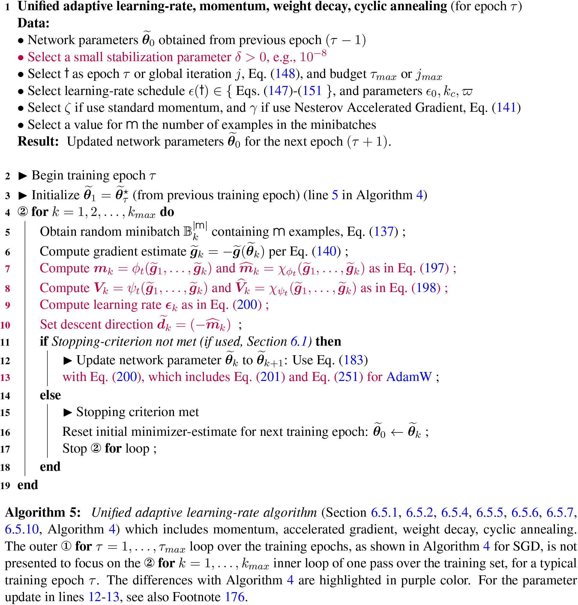
Remark 6.11. A particular case is the AdaDelta algorithm, in which
All of the above arrays—such as
where the Hadamard operator
Remark 6.12. The element-wise operations in Eq. (200) and Eq. (201) would allow each parameter in array
It remains to define the functions
SGD. To obtain Algorithm 4 as a particular case, select the following functions for Algorithm 5:
together with learning-rate schedule
Similarly for SGD with momentum and accelerated gradient (Section 6.3.2), step-length decay and cyclic annealing (Section 6.3.4), weight decay (Section 6.3.6).
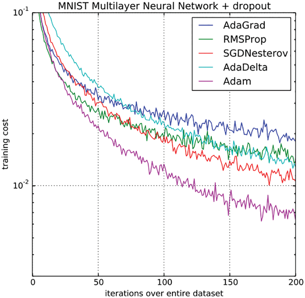
Figure 68: Convergence of adaptive learning-rate algorithms (Section 6.3.2): AdaGrad, RMSProp, SGDNesterov, AdaDelta, Adam [170]. (Figure reproduced with permission of the authors.)
6.5.2 AdaGrad: Adaptive Gradient
Starting the line of research on adaptive learning-rate algorithms, the authors of [52]182 selected the following functions for Algorithm 5:
leading to an update with adaptive scaling of the learning rate
in which each parameter in
Figure 68 shows the convergence of some adaptive learning-rate algorithms: AdaGrad, RMSProp, SGDNesterov, AdaDelta, Adam.
6.5.3 Forecasting time series, exponential smoothing
At this point, all of the subsequent adaptive learning-rate algorithms made use of an important technique in forecasting known as exponential smoothing of time series, without using this terminology, but instead referred to such technique as “exponential decaying average” [54], [78], p. 300, “exponentially decaying average” [80], “exponential moving average” [170], [182], [205], [162], “exponential weight decay” [56].

Figure 69: Dow Jones Industrial Average (DJIA, Section 6.5.3) stock index year-to-date (YTD) chart as from 2019.01.01 to 2019.11.30, Google Finance.
“Exponential smoothing methods have been around since the 1950s, and are still the most popular forecasting methods used in business and industry” such as “minute-by-minute stock prices, hourly temperatures at a weather station, daily numbers of arrivals at a medical clinic, weekly sales of a product, monthly unemployment figures for a region, quarterly imports of a country, and annual turnover of a company” [206]. See Figure 69 for the chart of a stock index showing noise.
“Exponential smoothing was proposed in the late 1950s (Brown, 1959; Holt, 1957; Winters, 1960), and has motivated some of the most successful forecasting methods. Forecasts produced using exponential smoothing methods are weighted averages of past observations, with the weights decaying exponentially as the observations get older. In other words, the more recent the observation the higher the associated weight. This framework generates reliable forecasts quickly and for a wide range of time series, which is a great advantage and of major importance to applications in industry” [207], Chap. 7, “Exponential smoothing”. See Figure 70 for an example of “exponential-smoothing” curve that is not “smooth”.
Figure 70: Saudi Arabia oil production during 1996-2013 (Section 6.5.3). Piecewise linear data (black) and fitted curve (red), despite the name “smoothing”. From [207], Chap. 7. (Figure reproduced with permission of the authors.)
For neural networks, early use of exponential smoothing dates back at least to 1998 in [165] and [166].185
For adaptive learning-rate algorithms further below (RMSProp, AdaDelta, Adam, etc.), let
Eq. (209) is a convex combination between
where the first term in Eq. (212) is called the bias, which is set by the initial condition:
For finite time
Eq. (212) is the discrete counterpart of the linear part of Volterra series in Eq. (497), used widely in neuroscientific modeling; see Remark 13.2. See also the “small heavy sphere” method or SGD with momentum Eq. (145).
It should be noted, however, that for forecasting (e.g., [207]), the following recursive equation, slightly different from Eq. (209), is used instead:
where
6.5.4 RMSProp: Root Mean Square Propagation
Since “AdaGrad shrinks the learning rate according to the entire history of the squared gradient and may have made the learning rate too small before arriving at such a convex structure”,186 The authors of [53]187 fixed the problem of continuing decay of the learning rate by introducing RMSProp188 with the following functions for Algorithm 5:
where the running average of the squared gradients is given in Eq. (216) for efficient coding, and in Eq. (217) in fully expanded form as a series with exponential coefficients
Figure 68 shows the convergence of some adaptive learning-rate algorithms: AdaGrad, RMSProp, SGDNesterov, AdaDelta, Adam.
RMSProp still depends on a global learning rate
6.5.5 AdaDelta: Adaptive Delta (parameter increment)
The name “AdaDelta” comes from the adaptive parameter increment
The weaknesses of AdaGrad was observed in [54]: “Since the magnitudes of gradients are factored out in AdaGrad, this method can be sensitive to initial conditions of the parameters and the corresponding gradients. If the initial gradients are large, the learning rates will be low for the remainder of training. This can be combatted by increasing the global learning rate, making the AdaGrad method sensitive to the choice of learning rate. Also, due to the continual accumulation of squared gradients in the denominator, the learning rate will continue to decrease throughout training, eventually decreasing to zero and stopping training completely.”
AdaDelta was then introduced in [54] as an improvement over AdaGrad with two goals in mind: (1) to avoid the continuing decay of the learning rate, and (2) to avoid having to specify
Thus, exponential smoothing (Section 6.5.3) is used for two second-moment series:
where
where the enclosing square brackets denote units (physical dimensions), but that was not the case in Eq. (218) of RMSProp:
Figure 68 shows the convergence of some adaptive learning-rate algorithms: AdaGrad, RMSProp, SGDNesterov, AdaDelta, Adam.
Despite this progress, AdaDelta and RMSProp, along with other adaptive learning-rate algorithms, shared the same pitfalls as revealed in [55].
Both both 1st moment Eq. (226) and 2nd moment Eq. (228) are adaptive. To avoid possible large step sizes and non-convergence of RMSProp, the following functions were selected for Algorithm 5 [170]:
with the following recommended values of the parameters:
Remark 6.13. RMSProp is a particular case of Adam, when
It follows from Eq. (212) in Section 6.5.3 on exponential smoothing of time series that the recurrence relation for gradients (1st moment) in Eq. (226) leads to the following series:
since
where
The argument to obtain the bias-corrected 2nd moment
The authors of [170] pointed out the lack of bias correction in RMSProp (Remark 6.13), leading to “very large step sizes and often divergence”, and provided numerical experiment results to support their point.
Figure 68 shows the convergence of some adaptive learning-rate algorithms: AdaGrad, RMSProp, SGDNesterov, AdaDelta, Adam. Their results show the superior performance of Adam compared to other adaptive learning-rate algorithms. See Figure 151 in Section 14.7 on “Lack of transparency and irreproducibility of results” in recent deep-learning papers.
6.5.7 AMSGrad: Adaptive Moment Smoothed Gradient
The authors of [182] stated that Adam (and other variants such as RMSProp, AdaDelta, Nadam) “failed to converge to an optimal solution (or a critical point in non-convex settings)” in many applications with large output spaces, and constructed a simple convex optimization for which Adam did not converge to the optimal solution.
An earlier version of [182] received one of the three Best Papers at the ICLR 2018191 conference, in which it was suggested to fix the problem by endowing the mentioned algorithms with “long-term memory” of past gradients, and by selecting the following functions for Algorithm 5:
The parameter
First-time learners in this field could be overwhelmed by complex-looking equations in this kind of paper, so it would be helpful to elucidate some key results that led to the above expressions, particularly for
It was stated in [182] that “one typically uses a constant
The second choice
where
where
where the following series expansion had been used:195
Comparing the bound on the right-hand side of (244) to the corresponding bound shown in [182], Corollary 1, second term, it can be seen that two factors,
On the other hand, there were some slight errors in the theorem statements and in the proofs in [182] that were corrected in [183], whose authors did a good job of not skipping any mathematical details that rendered the understanding and the verification of the proofs obscure and time consuming. It is then recommended to read [182] to get a general idea on the main convergence results of AMSGrad, then read [183] for the details, together with their variant of AMSGrad called AdamX.
The authors of [203], like those of [182], pointed out errors in the convergence proof in [170], and proposed a fix to this proof, but did not suggest any new variant of Adam.
In the two large numerical experiments on the MNIST dataset in Figure 71,196 the authors of [182] used contant
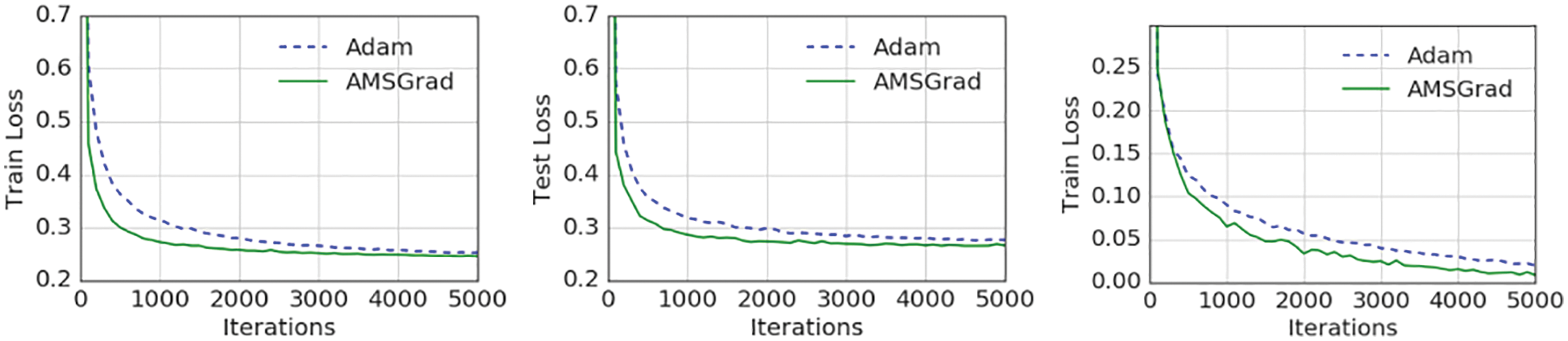
Figure 71: AMSGrad vs Adam, numerical examples (Sections 6.1, 6.5.7). The MNIST dataset is used. The first two figures on the left were the results of using logistic regression (network with one layer with logistic sigmoid activation function), whereas the figure on the right is by using a neural network with three layers (input layer, hidden layer, output layer). The cost function decreased faster for AMSGrad compared to that of Adam. For logistic regression, the difference between the two cost values also decreased with the iteration number, and became very small at iteration 5000. For the three-layer neural network, the cost difference between AMSGrad and Adam stayed more or less constant, as the cost went down to more than one tenth of the initial cost at about 0.3, and after 5000 iterations, the AMSGrad cost (
The authors of [182] also did not provide any numerical example with
Unfortunately, when comparing AMSGrad to Adam and AdamW (further below), it was remarked in [209] that AMSGrad generated “a lot of noise for nothing”, meaning AMSGrad did not live up to its potential and best-paper award when tested on “real-life problems”.
6.5.8 AdamX and Nostalgic Adam
AdamX. The authors of [183], already mentioned above in connection to errors in the proofs in [182] for AMSGrad, also pointed out errors in the proofs by [170] (Theorem 10.5), [203] (Theorem 4.4), and by others, and suggested a fix for these proofs, and a new variant of AMSGrad called AdamX.
Reference [183] is more convenient to read, compared to [182], as the authors provided all mathematical details for the proofs, without skipping important details.
A slight change to Eq. (240) was proposed in [183] as follows:
In addition, numerical examples were provided in [183] with
Nostalgic Adam. The authors of [204] also fixed the non-convergence of Adam by introducing “long-term memory” to the second-moment of the gradient estimates, similar to the work in [182] on AMSGrad and in [183] on AdamX.
There are many more variants of Adam. But how are Adam and its variants compared to good old SGD with new add-on tricks ? (See the end of Section 6.3.1)
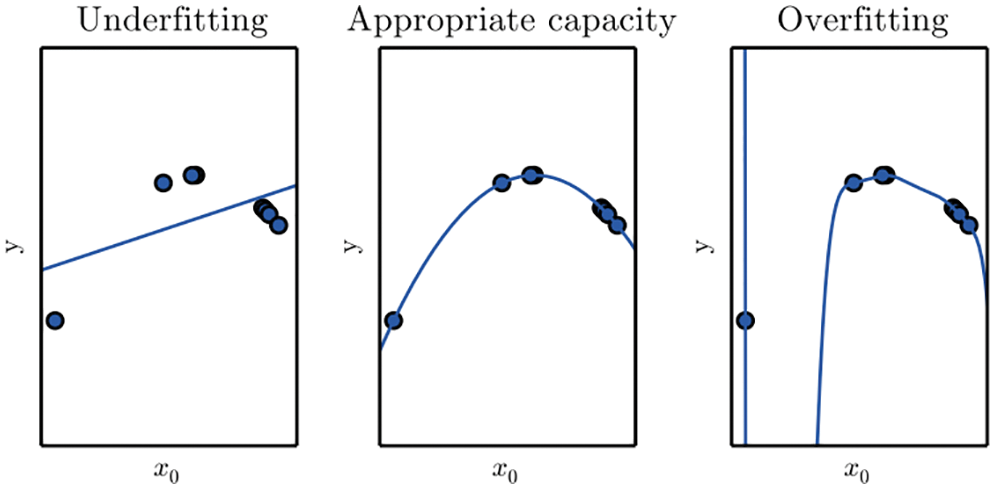
Figure 72: Overfitting (Section 6.5.9, 6.5.10). Left: Underfitting with 1st-order polynomial. Middle: Appropriate fitting with 2nd-order polynomial. Right: Overfitting with 9th-order polynomial. See [78], p. 110, Figure5.2. (Figure reproduced with permission of the authors.)
6.5.9 Criticism of adaptive methods, resurgence of SGD
Yet, despite the claim that RMSProp is “currently one of the go-to optimization methods being employed routinely by deep learning practitioners,” and that “currently, the most popular optimization algorithms actively in use include SGD, SGD with momentum, RMSProp, RMSProp with momentum, AdaDelta, and Adam”,197 the authors of [55] through their numerical experiments, that adaptivity can overfit (Figure 72), and that standard SGD with step-size tuning performed better than adaptive learning-rate algorithms such as AdaGrad, RMSProp, and Adam. The total number of parameters,
making it prone to overfit without employing special techniques such as regularization or weight decay (see AdamW below).
It was observed in [55] that adaptive methods tended to have larger generalization (test) errors199 compared to SGD: “We observe that the solutions found by adaptive methods generalize worse (often significantly worse) than SGD, even when these solutions have better training performance,” (see Figure 73), and concluded that:
“Despite the fact that our experimental evidence demonstrates that adaptive methods are not advantageous for machine learning, the Adam algorithm remains incredibly popular. We are not sure exactly as to why, but hope that our step-size tuning suggestions make it easier for practitioners to use standard stochastic gradient methods in their research.”
The work of [55] has encouraged researchers who were enthusiastic with adaptive methods to take a fresh look at SGD again to tease something more out of this classic method.200
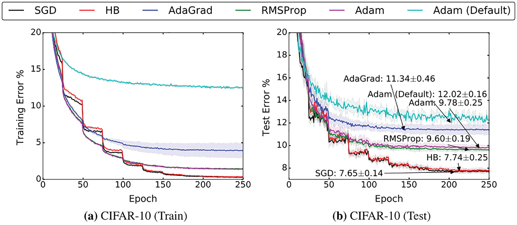
Figure 73: Standard SGD and SGD with momentum vs. AdaGrad, RMSProp, Adam on CIFAR-10 dataset (Sections 6.1, 6.3.2, 6.5.9). From [55], where a method for step-size tuning and step-size decaying was proposed to achieve lowest training error and generalization (test) error for both Standard SGD and SGD with momentum (“Heavy Ball” or better yet “Small Heavy Sphere” method) compared to adaptive methods such as AdaGrad, RMSProp, Adam. (Figure reproduced with permission of the authors.)
6.5.10 AdamW: Adaptive moment with weight decay
The authors of [56], aware of the work in [55], wrote: It was suggested in [55] “that adaptive gradient methods do not generalize as well as SGD with momentum when tested on a diverse set of deep learning tasks, such as image classification, character-level language modeling and constituency parsing.” In particular, it was shown in [56] that “ a major factor of the poor generalization of the most popular adaptive gradient method, Adam, is due to the fact that
Briefly, “
The magnitude of the coefficient
and the update becomes:
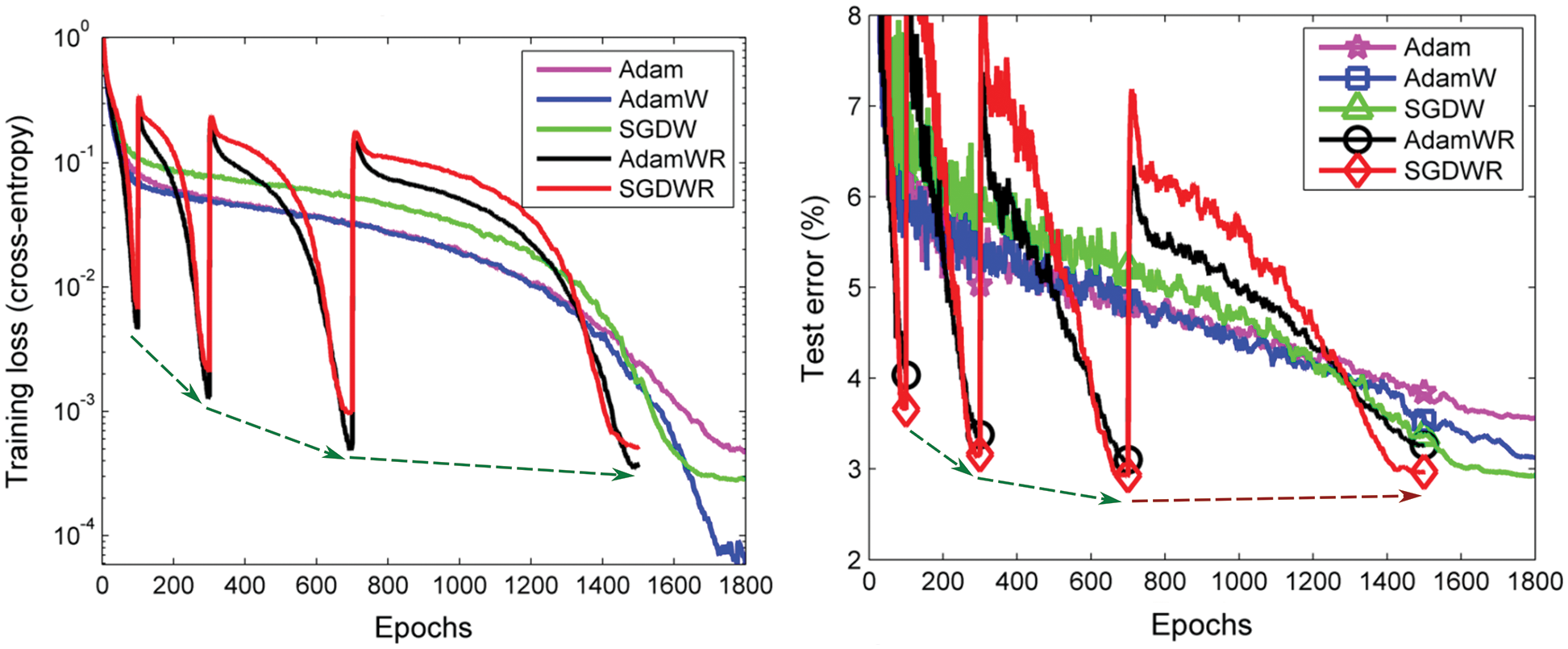
Figure 74: AdamW vs Adam, SGD, and variants on CIFAR-10 dataset (Sections 6.1, 6.5.10). While AdamW achieved lowest training loss (error) after 1800 epochs, the results showed that SGD with weight decay (SGDW) and with warm restart (SGDWR) achieved lower test (generalization) errors than Adam, AdamW, AdamWR. See Figure 75 for the scheduling of the annealing multiplier
which is equivalent to decaying the parameters (including the weights in)
The same equivalence between
where the parameter
The results of the numerical experiments on the CIFAR-10 dataset using Adam, AdamW, SGDW (Weight decay), AdamWR (Warm Restart), and SGDWR were reported in Figure 74 [56].
Remark 6.14. Limitation of cyclic annealing. The 5th cycle of annealing not shown in Figure 74 would end at epoch
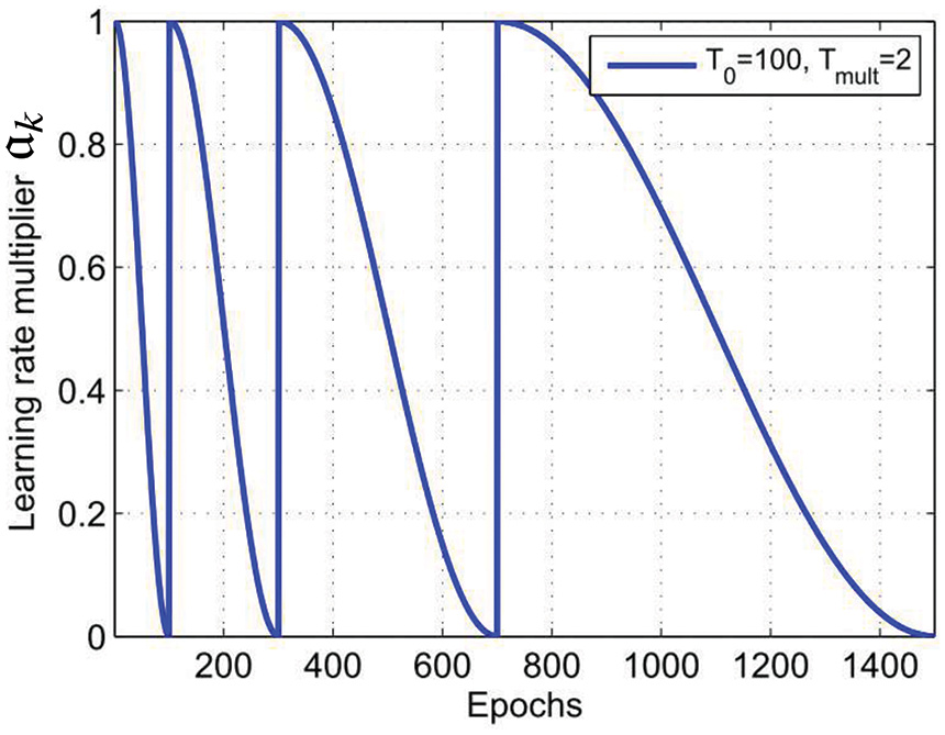
Figure 75: Cosine annealing (Sections 6.3.4, 6.5.10). Annealing factor
The results for test errors in Figure 74 appeared to confirm the criticism in [55] that adaptive methods brought about “marginal value” compared to the classic SGD. Such observation was also in agreement with [168], where it was stated:
“In our experiments, either AdaBayes or AdaBayes-SS outperformed other adaptive methods, including AdamW (Loshchilov & Hutter, 2017), and Ada/AMSBound (Luo et al., 2019), though SGD frequently outperformed all adaptive methods.” (See Figure 76 and Figure 77)
If AMSGrad generated “a lot of noise for nothing” compared to Adam and AdamW, according to [209], then does “marginal value” mean that adaptive methods in general generated a lot of noise for not much, compared to SGD ?
The work in [55], [168], and [56] proved once more that a classic like SGD introduced by Robbins & Monro (1951b) [49] never dies, and would be motivation to generalize classical deterministic first and second-order optimization methods together with line search methods to add stochasticity. We will review in detail two papers along this line: [144] and [145].
6.6 SGD with Armijo line search and adaptive minibatch
In parallel to the deterministic choice of step length based on Armijo’s rule in Eq. (125) and Eq. (126), we have the following respective stochastic version proposed by [144]:202
Figure 76: CIFAR-100 test loss using Resnet-34 and DenseNet-121 (Section 6.5.10). Comparison between various optimizers, including Adam and AdamW, showing that SGD achieved the lowest global minimum loss (blue line) compared to all adaptive methods tested as shown [168]. See also Figure 77 and Section 6.1 on early-stopping criteria. (Figure reproduced with permission of the authors.)
Figure 77: SGD frequently outperformed all adaptive methods (Section 6.5.10). The table contains the global minimum for each optimizer, for each of the two datasets CIFAR-10 and CIFAR-100, using two different networks. For each network, an error percentage and the loss (cost) were given. Shown in red are the lowest global minima obtained by SGD in the corresponding columns. Even in the three columns in which SGD results were not the lowest, two SGD results were just slightly above those of AdamW (1st and 3rd columns), and one even smaller (4th column). SGD clearly beat Adam, AdaGrad, AMSGrad [168]. See also Figure 76. (Figure reproduced with permission of the authors.)
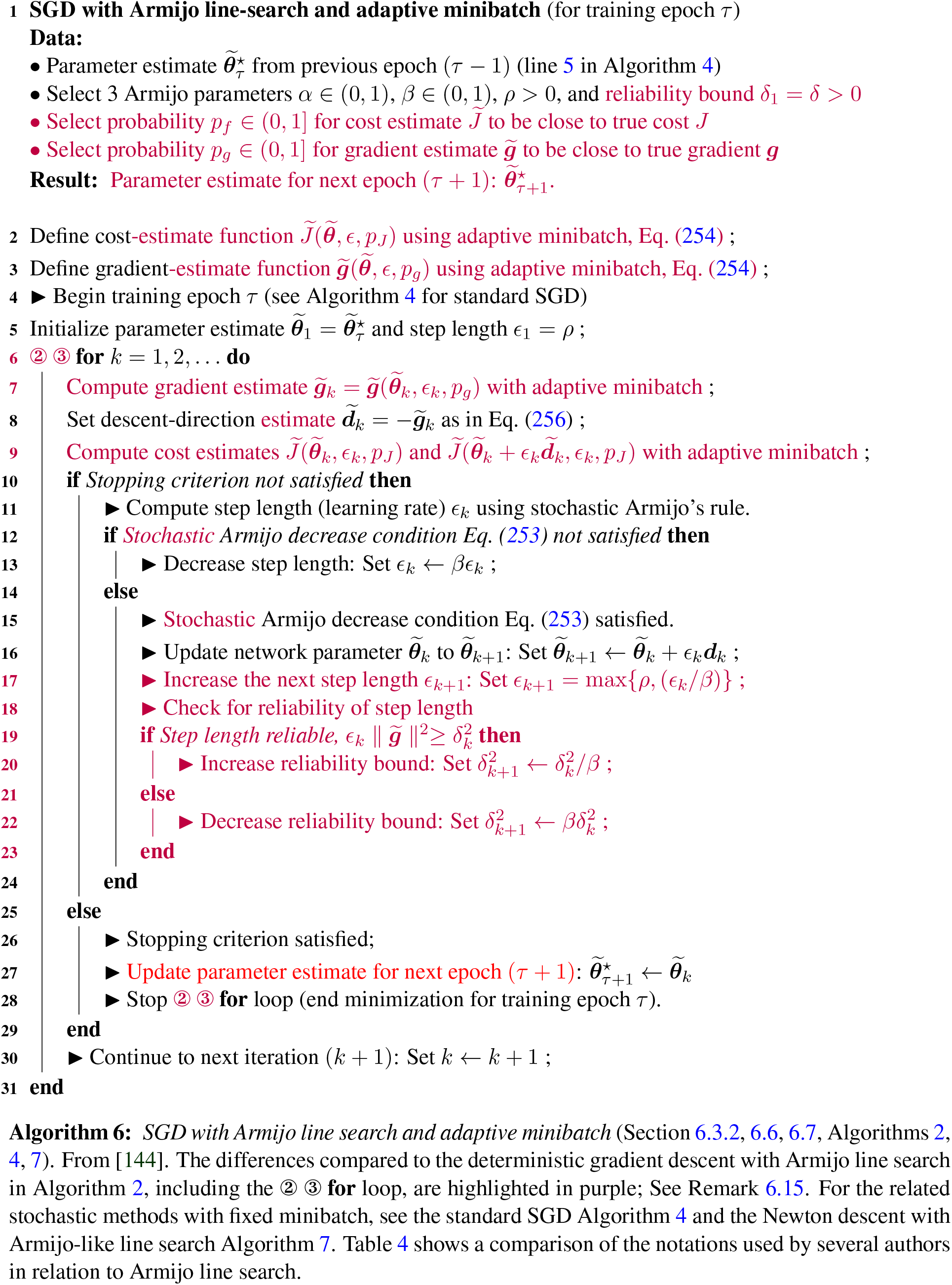
where the overhead tilde of a quantity designates an estimate of that quantity based on a randomly selected minibatch, i.e.,
There is a difference though: The standard SGD in Algorithm 4 uses a fixed minibatch for the computation of the cost estimate and the gradient estimate, whereas Algorithm 6 in [144] uses adaptive subprocedure to adjust the size of the minibatches to achieve a desired (fixed) probability
which are the counterparts to the fixed-minibatch procedures in Eq. (139) and Eq. (140), respectively.
Remark 6.15. Since the appropriate size of the minibatch depends on the gradient estimate, which is not known and which is computed based on the minibatch itself, the adaptive-minibatch subprocedures for cost estimate
In addition, since both the cost estimate
The same relationship between
For SGD, the descent-direction estimate
For Newton-type algorithms, such as in [145] [146], the descent direction estimate
Remark 6.16. In the SGD with Armijo line search and adaptive minibatch Algorithm 6, the reliability parameter
The authors of [144] provided a rigorous convergence analysis of their proposed Algorithm 6, but had not implemented their method, and thus had no numerical results at the time of this writing.204 Without empirical evidence that the algorithm works and is competitive compared to SGD (see adaptive methods and their criticism in Section 6.5.9), there would be no adoption.
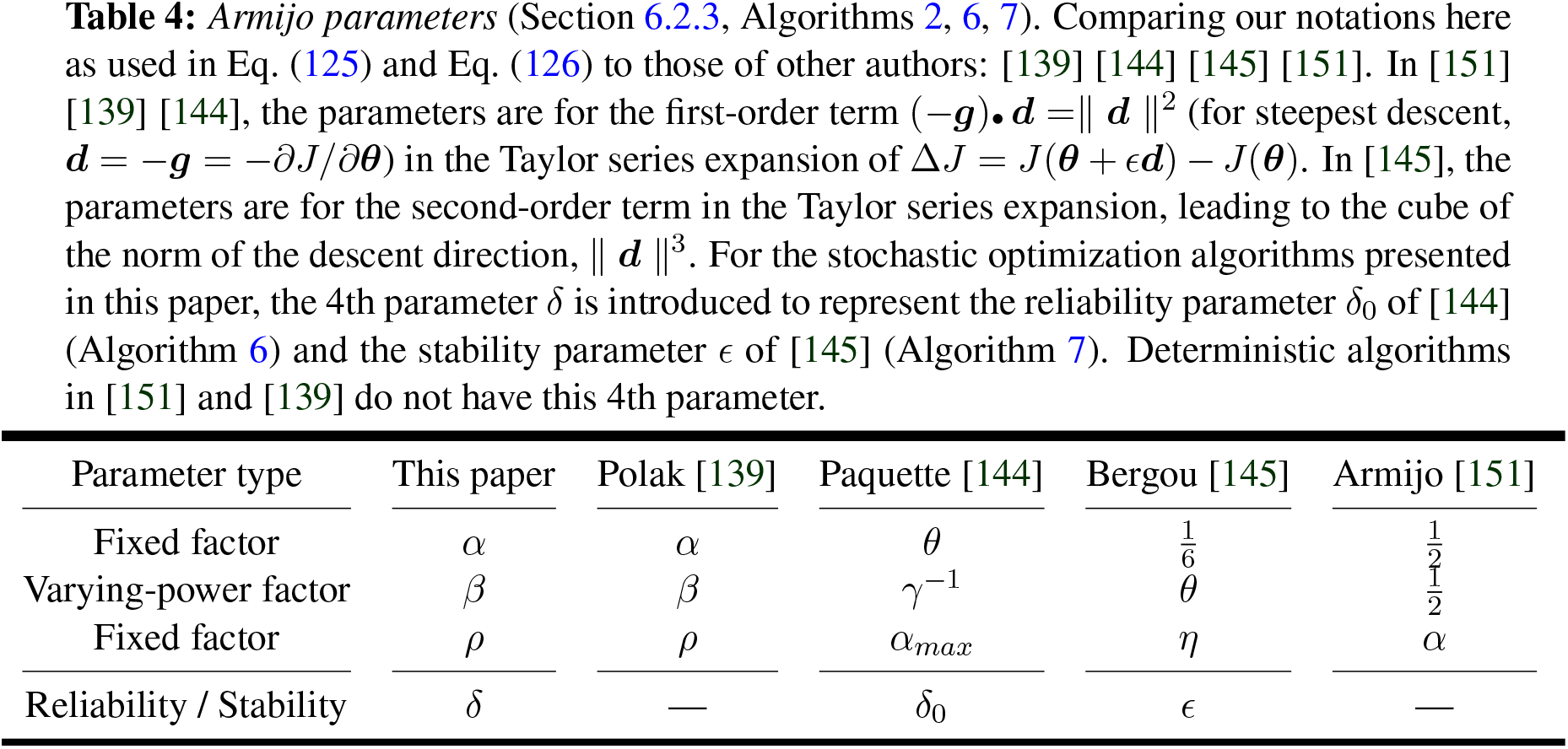
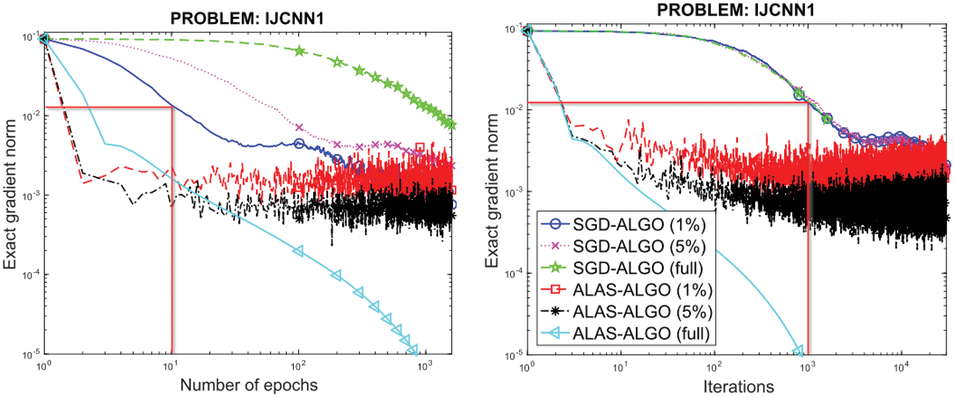
Figure 78: Stochastic Newton with Armijo-like 2nd order line search (Section 6.7). IJCNN1 dataset from the LIBSVM library. Three batch sizes were used (1%, 5%, 100%) for both SGD and ALAS (stochastic Newton Algorithm 7). The exact gradient norm for each of these six cases was plotted against the training epochs on the left, and against the iteration numbers on the right. An epoch is the number of non-overlapping minibatches (and thus iterations) to cover the whole training set. One epoch for a minibatch size of s% (respectively 1%, 5%, 100%) of the training set is equivalent to 100/s (respectively 100, 20, 1) iterations. Thus, for SGD-ALGO (1%), as shown, 10 epochs is equivalent to 1,000 iterations, with the same gradient norm. The markers on the curves were placed every 100 epochs (left) and 800 iterations (right). For the same number of epochs, say 10, SGD with smaller minibatches yielded lower gradient norm. The same was true for Algorithm 7 for number of epochs less than 10, but the gradient norm plateaued out after that with a lot of noise. Second-order Algorithm 7 converged faster than 1st-order SGD. See [145]. (Figure reproduced with permission of the authors.)
6.7 Stochastic Newton method with 2nd-order line search
The stochastic Newton method in Algorithm 7, described in [145], is a generalization of the deterministic Newton method in Algorithm 3 to add stochasticity via random selection of minibatches and Armijo-like 2nd-order line search.205
Upon a random selection of a minibatch as in Eq. (137), the computation of the estimates for the cost function
In the above computation, the minibatch in Algorithm 7 is fixed, not adaptive such as in Algorithm 6.
If the current iterate
where
If the current iterate
then find the eigenvector
When the iterate
The remaining case is when the iterate
If the stopping criterion is not met, use Armijo’s rule to find the step length
From Eq. (125), the deterministic 1st-order Armijo’s rule for steepest descent can be written as:
with
with
Figure 78 shows the numerical results of Algorithm 7 on the IJCNN1 dataset ([211]) from the Library for Vector Support Machine (LIBSVM) library by [212]. It is not often to see plots versus epochs side by side with plots versus iterations. Some papers may have only plots versus iterations (e.g., [182]); other papers may rely only on plots versus epochs to draw conclusions (e.g., [56]). Thus Figure 78 provides a good example to see the differences, as noted in Remark 6.17.
Remark 6.17. Epoch counter vs global iteration counter in plots. When plotted gradient norm versus epochs (left of Figure 78), the three curves for SGD were separated, with faster convergence for smaller minibatch sizes Eq. (135), but the corresponding three curves fell on top of each other when plotted versus iterations (right of Figure 78). The reason was the scale on the horizontal axis was different for each curve, e.g., 1 iteration for full batch was equivalent to 100 iterations for minibatch size at 1% of full batch. While the plot versus iterations was the zoom-in view, but for each curve separately. To compare the rates of convergence among different algorithms and different minibatch sizes, look at the plots versus epochs, since each epoch covers the whole training set. It is just an optical illusion to think that SGD with different minibatch sizes had the same rate of convergence. ■
The authors of [145] planned to test their Algorithm 7 on large datasets such as the CIFAR-10, and report the results in 2020.207
Another algorithm along the same line as Algorithm 6 and Algorithm 7 is the stochastic quasi-Newton method proposed in [146], where the stochastic Wolfe line search of [143] was employed, but with no numerical experiments on large datasets such as CIFAR-10, etc.
At the time of this writing, due to lack of numerical results with large datasets commonly used in the deep-learning community such as CIFAR-10, CIFAR-100 and the likes, for testing, and thus lack of comparison of performance in terns of cost and accuracy against Adam and its variants, our assessment is that SGD and its variants, or Adam and its better variants, particularly AdamW, continue to be the prevalent methods for training.
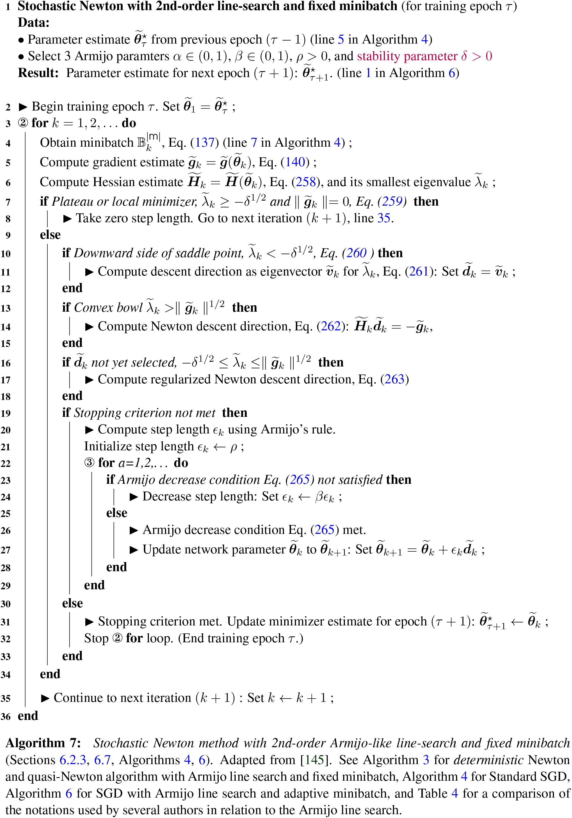
Time constraint did not allow us to review other stochastic optimization methods such as that with the gradient-only line search in [142] and [179] could not be reviewed here.
7 Dynamics, sequential data, sequence modeling
7.1 Recurrent Neural Networks (RNNs)
In many fields of physics, the respective governing equations that describe the response of a system to (external) stimuli follow a common pattern. The temporal and/or spatial change of some quantity of a system is balanced by sources that cause the change, which is why we refer to equations of this kind as balance relations. The balance of linear momentum in mechanics, for instance, establishes a relationship between the temporal change of a body’s linear momentum and the forces acting on the body. Along with kinematic relations and constitutive laws, the balance equations provide the foundation to derive the equations of motion of some mechanical system. For linear problems, the equations of motion constitute a system of second-order ODEs in appropriate (generalized) coordinates
In the above equation,
In control theory,
we obtain a compact representation of the equations of motion, which relates the temporal change of the system’s state
We found similar relations in neuroscience,209 where the dynamics of neurons was accounted for, e.g., in the pioneering work [214], whose author modeled a neuron as electrical circuit with capacitances. Time-continuous RNNs were considered in a paper on back-propagation [215]. The temporal change of an RNN’s state is related to the current state
where
Returning to mechanics, we are confronted with the problem that the equations of motion do not admit closed-form solutions in general. To construct approximate solution, time-integration schemes need to be resorted to, where we mention a few examples such as Newmark’s method [216], the Hilber-Hughes-Taylor (HHT) method [217], and the generalized-
Rearranging the above relation for the new state gives the update equation for the state vector,
which determines the next state
which allows us to rewrite Eq. (272) as
The update equation of time-discrete RNNs is similar to the discretized equations of motion Eq. (274). Unlike feed-forward neural networks, the state
Remark 7.1. In [78], there is a distinction between the “hidden state” of an RNN cell at the
The above relation is illustrated as a circular graph in Figure 79 (left), where the delay is explicit in the superscript of
Continuing this unfolding process repeatedly until we reach the beginning of a sequence, the recurrence can be expressed as a function
which takes the entire sequence up to the current step
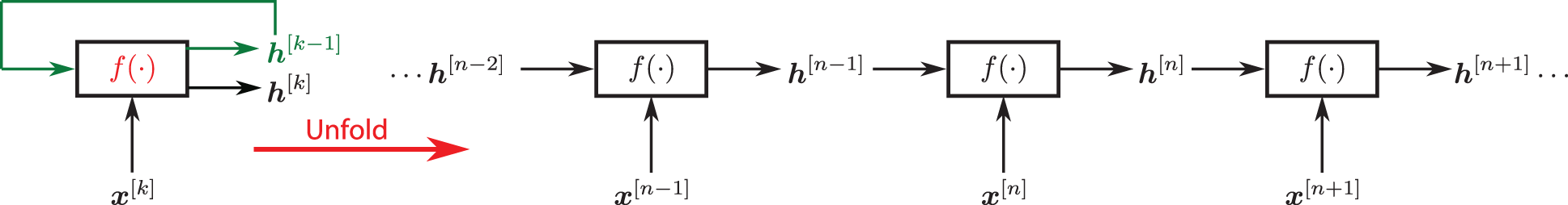
Figure 79: Folded and unfolded discrete RNN (Section 7.1, 13.2.2). Left: Folded discrete RNN at configuration (or state) number
As an example, consider the default (“vanilla”) single-layer RNN provided by PyTorch214 and TensorFlow215, which is also described in [78], p. 370:
First,
A common design pattern of RNNs adds a linear output layer to the simplistic example in Figure 79, i.e., the RNN has a recurrent connection between its hidden units, which represent the state
and the second layer forms a linear combination of the first layer’s output
which was given in Eq. (84); see [78], p. 369. The parameters of the network are the weight matrices
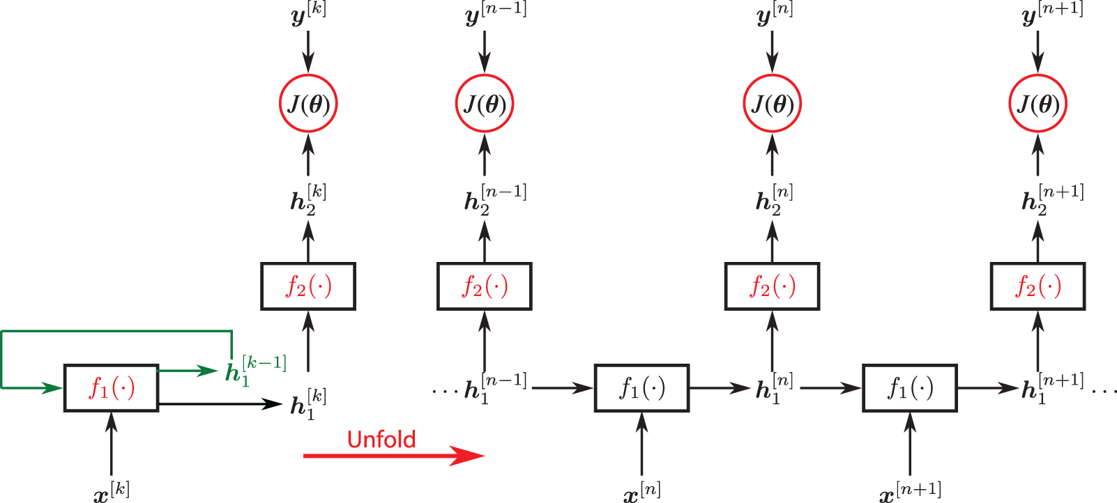
Figure 80: RNN with two multilayer neural networks (MLNs), (Section 7.1) denoted by
Irrespective of the number of layers, the hidden state
Other design patterns for RNNs show, e.g., recurrent connections between the hidden units but produce a single output only. RNNs may also have recurrent connections from the output at one time step to the hidden unit of next time step.
Comparing the recurrence relation in Eq. (277) and its unfolded representation in Eq. (278), we can make the following observations:
• The unfolded representation after
• The same transition function
• A state
Remark 7.2. Depth of RNNs. For the above reasons and Figures 79-80, “RNNs, once unfolded in time, can be seen as very deep feedforward networks in which all the layers share the same weights” [13]. See Section 4.6.1 on network depth and Remark 4.5. ■
By nature, RNNs are typically employed for the processing of sequential data
Comparing the update equations Eq. (274) and Eq. (279), we note the close resemblance of dynamic systems and RNNs. Let aside the non-linearity of the activation function and the presence of the bias vector, both have state vectors with recurrent connections to the previous states. Employing the trapezoidal rule for the time-discretization, we find a recurrence in the input, which is not present in the type of RNNs described above. The concept of parameter sharing in RNNs translates into the notion of time-invariant systems in dynamics, i.e., the state matrix
The crucial challenge in RNNs is to learn long-term dependencies, i.e., relations among distant elements in input sequences. For long sequences, we face the problem of vanishing or exploding gradients when training the network by means of back-propagation. To understand vanishing (or exploding) gradients, we can draw analogies between RNNs and dynamic systems once again. For this purpose, we consider an RNN without inputs whose activation function is the identity function:
From the dynamics point of view, the above update equation corresponds to a linear autonomous system, whose time-discrete representation is given by
Clearly, the equilibrium state of the above system is the trivial state
If eigenvalues of
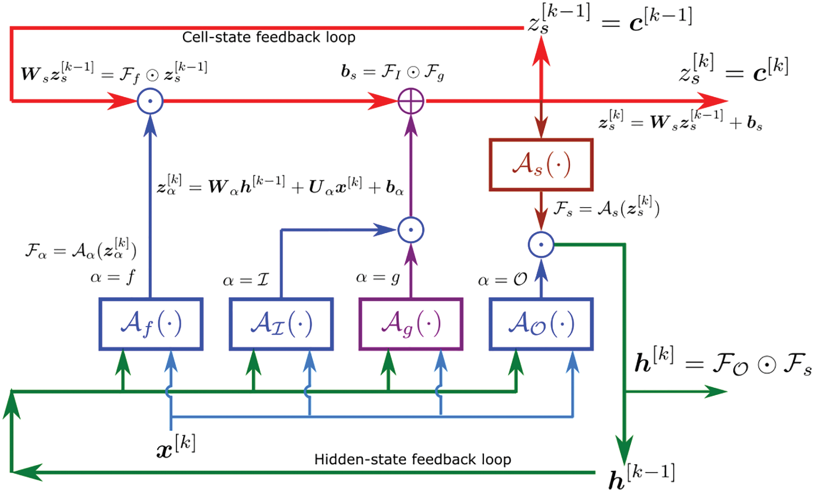
Figure 81: Folded Recurrent Neural Network (RNN) with Long Short-Term Memory (LSTM) cell (Section 7.2, 11.3.3). The cell state at
7.2 Long Short-Term Memory (LSTM) unit
The vanishing (exploding) gradient problem prevents us from effectively learning long-term dependencies in long input sequences by means of conventional RNNs. Gated RNNs as the long short-term memory (LSTM) and networks based on the gated recurrent unit (GRU) have proven to successfully overcome the vanishing gradient problem in diverse applications. The common idea of gated RNNs is to create paths through time along which gradients neither vanish nor explode. Gated RNNs can accumulate information in their state over many time steps, but, once the information has been used, they are capable to forget their state by, figuratively speaking, “closing gates” to stop the information flow. This concept bears a resemblance to residual networks, which introduce skip connections to circumvent vanishing gradients in deep feed-forward networks; see Section 4.6.2 on network “Architecture”.
Remark 7.3. What is “short-term” memory? The vanishing gradient at the earlier states of an RNN (or layers in the case of a multilayer neural network) makes it that information in these earlier states (or layers) did not propagate forward to contribute to adjust the predicted outputs to track the labeled outputs, so to decrease the loss. A state
In their pioneering work on LSTM, the authors of [24] presented a mechanism that allows information (inputs, gradients) to flow over a long duration by introducing additional states, paths and self-loops. The additional components are encapsulated in so-called LSTM cells. LSTM cells are the building blocks for LSTM networks, where they are connected recurrently to each other analogously to hidden neurons in conventional RNNs. The introduction of a cell state219
Another way to explain that could contribute to elucidate the concept is: Since information in RNN cannot be stored for a long time, over many subsequent steps, LSTM cell corrected this short-term memory problem by remembering the inputs for a long time:
“A special unit called the memory cell acts like an accumulator or a gated leaky neuron: it has a connection to itself at the next time step that has a weight of one, so it copies its own real-valued state and accumulates the external signal, but this self-connection is multiplicatively gated by another unit that learns to decide when to clear the content of the memory.” [13].
In a unified manner, the various relations in the original LSTM unit depicted in Figure 81 can be expressed in a single key generic recurring-relation that is more easily remembered:
where
In Figure 81, two types of squashing functions are used: One type (three blue boxes with
Remark 7.4.The activation function
There are two feedback loops, each with a delay by one step. The cell-state feedback loop (red) at the top involves the LSTM cell state
In the hidden-state feedback loop (green) at the bottom, the combination
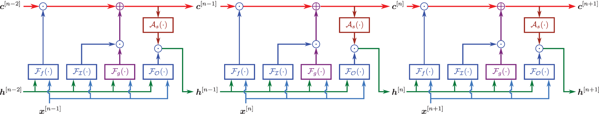
Figure 82: Unfolded RNN with LSTM cells (Sections 2.3.2, 7.2, 12.1): In this unfolded RNN, the cell states are centered at the LSTM cell
As the term suggests, the presence of gates that control the information flow are a further key concept in gated RNNs and LSTM, in particular. Gates are constructed from a linear layer with a sigmoidal function (logistic sigmoid or hyperbolic tangent) as activation function that squashes the components of a vector into the range
To understand the function of LSTM, we follow the paths information is routed through an LSTM cell. At time
The weights associated with the hidden state and the cell state are
Again,
The actual updates are determined by a component-wise multiplication of the candidate values
The new cell state
where the component-wise multiplication of matrices, which is also known by the name Hadamard product, is indicated by a “
Remark 7.5.The path of the cell state
Finally, the hidden state of the LSTM cell is computed from the cell state
before the result
Hence, the output, i.e., the new hidden state
For the LSTM cell, we get an intuition for respective choice of the activation function. The hyperbolic tangent is used to normalize and center information that is to be incorporated into the cell state or the hidden state. The forget gate, input gate and output gate make use of the sigmoid function, which takes values between 0 and 1, to either discard information or allow information to pass by.
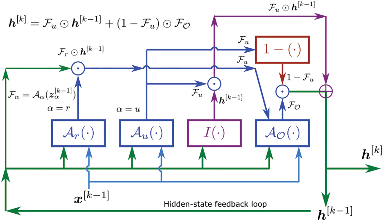
Figure 83: Folded RNN with Gated Recurrent Unit (GRU) (Section 7.3). The cell state at
7.3 Gated Recurrent Unit (GRU)
In a unified manner, the various relations in the GRU depicted in Figure 83 can be expressed in a single key generic recurring-relation similar to the LSTM Eq. (286):
where
To facilitate a direct comparison between the GRU cell and the LSTM cell, the locations of the boxes (gates) in the GRU cell in Figure 83 are identical to those in the LSTM in Figure 81. It can be observed that in the GRU cell (1) There is no feedback loop for the cell state, (2) The input is
The GRU was introduced in [220], and tested against LSTM and tanh-RNN in [221], with concise GRU schematics, and thus not easy to follow, unlike Figure 83. The GRU relations below follow [78], p. 400.
The hidden variable
For the GRU update-gate effect
For the GRU output-gate effect
For the GRU reset-gate effect
Remark 7.6.GRU has fewer activation functions compared to LSTM, and is thus likely to be more efficient, even though it was stated in [221] that no concrete conclusion could be made as to “which of the two gating units was better.” See Remark 7.7 on the use of GRU to solve hyperbolic problems with shock waves. ■
7.4 Sequence modeling, attention mechanisms, Transformer
RNN and LSTM have been well-established for use in sequence modeling and “transduction” problems such as language modeling and machine translation. Attention mechanism, introduced in [57] [222], allowed for “modeling of dependencies without regard to their distance in the input and output sequences,” and has been used together with RNNs [31]. Transformer is a much more efficient architecture that only uses an attention mechanism, but without the RNN architecture, to “draw global dependencies between input and output.” Each of these concepts is discussed in detail below.
7.4.1 Sequence modeling, encoder-decoder
The term neural machine translation describes the approach of using a single neural network to translate a sentence.220 Machine translation is a special kind of sequence-to-sequence modeling problem, in which a source sequence is “translated” into a target sequence. Neural machine translation typically relies on encoder–decoder architectures.221
The encoder network converts (encodes) the essential information of the input sequence
To make things clearer, we briefly sketch the structure of a typical RNN encoder-decoder model following [57]. The encoder
In Section 7.1, we referred to
Note that
From a probabilistic point of view, the joint probability of the entire output sequence (i.e., the “translation”)
Accordingly, the decoder is trained to predict the next item (word, character) in the output sequence
To predict the conditional probability of the next item
We have various choices of how the context vector
As the authors of [57] emphasized, the encoder “needs to be able to compress all the necessary information of a source sentence into fixed-length vector”. For this reason, long sentences pose a challenge in neural machine translation, in particular, as sentences to be translated are longer than the sentences networks have seen during training, which was confirmed by the observations in [223]. To cope with long sentences, an encoder–decoder architecture, “which learns to align and translate jointly,” was proposed in [57]. Their approach is motivated by the observation that individual items of the target sequence correspond to different parts of the source sequence. To account for the fact that only a subset of the source sequence is relevant when generating a new item of the target sequence, two key ingredients (alignment and translation) to the conventional encoder–decoder architecture described above were introduced in [57], and will be presented below.
☛ The first key ingredient to their concept of “alignment” is the idea of using a distinct context vector
as is the conditional probability of the output items, Eq. (303),
i.e., it is conditioned on distinct context vectors
The
The
For this reason, using a bidirectional RNN225 as encoder was proposed in [57]. A bidirectional RNN combines two RNNs, i.e., a forward RNN and backward RNN, which independently process the source sequence in the original and in reverse order, respectively. The two RNNs generate corresponding sequences of forward and backward hidden states,
In each step, these vectors are concatenated to a single hidden state vector
They mentioned “the tendency of RNNs to better represent recent inputs” as reason why the annotation
☛ As the second key ingredient, the authors of [57] proposed a so-called “alignment model”, i.e., a function
which is meant to quantify (“score”) the relation, i.e., the alignment, between the
The alignment model is represented by a feedforward neural network, which is jointly trained along with all other components of the encoder–decoder architecture. The weights of the annotations, in turn, follow from the alignment scores upon exponentiation and normalization (through
The weighting in Eq. (306) is interpreted as a way “to compute an expected annotation, where the expectation is over possible alignments" [57]. From this perspective,
In neural machine translation it was possible to show that the attention model in [57] significantly outperformed conventional encoder–decoder architectures, which encoded the entire source sequence into a single fixed-length vector. In particular, this proposed approach turned out to perform better in translating long sentences, where it could achieve performance on par with phrase-based statistical machine translation approaches of that time.
7.4.3 Transformer architecture
Despite improvements, the attention model in [57] shared the fundamental drawback intrinsic to all RNN-based models: The sequential nature of RNNs is adverse to parallel computing making training less efficient as with, e.g., feed-forward or convolutional neural networks, which lend themselves to massive parallelization. To overcome this drawback, a novel model architecture, which entirely dispenses with recurrence, was proposed in [31]. As the title “Attention Is All You Need” already reveals, their approach to neural machine translation is exclusively based on the concept of attention (and some feedforward-layers), which is repeatedly used in the proposed architecture referred to as “Transformer”.
In what follows, we describe the individual components of the Transformer architecture, see Figure 85. Among those, the scaled dot-product attention, see Figure 84, is a fundamental building block. Scaled-dot product attention, which is represented by a function
Let
Scaling with the square root of the query/key dimension is supposed to prevent pushing the
Note that
Based on the concept of scaled dot-product attention, the idea of using multiple attention functions in parallel rather than just a single one was proposed in [31], see Figure 84. In their concept of “Multi-Head Attention”, each “head” represents a separate context
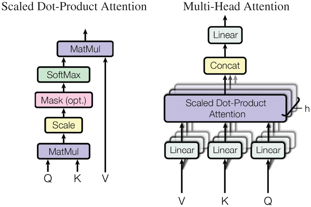
Figure 84: Scaled dot-product attention and multi-head attention (Section 7.4.3). Scaled-dot product attention (left) is the elementary building block of the Transformer model. It compares query vectors (Q) against a set of key vectors (K) to produce a context vector by weighting to value vectors (V) that correspond to the keys. For this purpose,
Multi-head attention combines the individual “heads”
where
To understand why the projection is essential in the Transformer architecture, we shift our attention (no pun intended) to the encoder-structure illustrated in Figure 85. The encoder combines a stack of
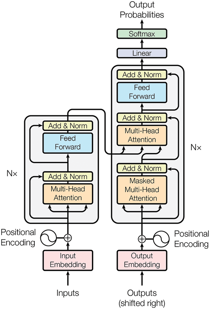
Figure 85: Transformer architecture (Section 7.4.3). The Transformer is a sequence-to-sequence model without recurrent connections. Encoder and decoder are entirely built upon scaled dot-product attention. Items of source and target sequences are numerically represented as vectors, i.e., embeddings. Positional encodings furnish embeddings with information on their positions within the respective sequences. The encoder stack comprises
In the context of multi-head attention, self-attention implies that one and the same sequence multiply serves as queries, keys and values, respectively. Let
The authors of [31] introduced a residual connection around the self-attention (sub-)layer, which, in view of the same dimensions of heads and queries, reduces to a simple addition.
To prevent values from growing upon summation, the residual connection is followed by layer normalization as proposed in [225], which scales the input to zero mean and unit variance:
where
The output of the first sub-layer is the input to the second sub-layer within the encoder stack, i.e., a “position-wise feed-forward network.” Position-wise means that a fully connected feedforward network (see Section 4 on “Static, feedforward networks”), which is subsequently represented by the function
where
As for the first sub-layer, the authors of [31] introduced a residual connection followed by layer normalization around the feedforward network. The ouput of the encoder’s second sublayer, which, at the same time, is the output of the encoder layer, is given by
Within the transformer architecture (Figure 85), the encoder is composed from
or, alternatively, using a step-wise representation,
Note that inputs and outputs of all components of an encoder layer share the same dimensions, which facilitates several layers to be stacked without additional projections in between.
The decoder’s structure within the transformer architecture is similar to that of the encoder, see the right part in Figure 85. As the encoder, it is composed from
Let
The second sub-layer relates items of the source and the target sequences by means of multi-head attention:
The third sub-layer is a fully-connected feed-forward network (with a single hidden layer) that is applied to each element of the sequence (position-wisely)
The output of the last (
A Transformer-model is trained on the complete source and target sequences, which are input to the encoder and the decoder, respectively. The target sequence is shifted right by one position, such that a special token indicating the start of a new sequence can be placed at the beginning, see Fig. 85. To prevent the decoder from attending to future items of the output sequence, the (multi-headed) self-attention sub-layer needs to be “masked”. The masking is realized by setting those inputs to the
As the transformer architecture does not have recurrent connections, positional encodings were added to the inputs of both encoder and decoder [31], see Figure 85. The positional encodings supply the individual items of the inputs to the encoder and the decoder with information about their positions within the respective sequences. For this purpose, the authors of [31] proposed to add vector-valued positional encodings
The trained Transformer-model produces one item of the output sequence at a time. Given the input sequence and all outputs already generated in previous steps, the Transformer predicts probabilities for the next item in the output sequence. Models of this kind are referred to as “auto-regressive”.
The authors of [31] varied parameters of the Transformer model to study the importance of individual components. Their “base model” used
As of 2022, the Generative Pre-trained Transformer 3 (GPT-3) model [226], which is based on the Transformer architecture, belongs to the most powerful language models. GPT-3 is an autoregressive model that produces text from a given (initial) text prompt, whereby it can deal with different tasks as translation, question-answering, cloze-tests228 and word-unscrambling, for instance. The impressive capabilities of GPT-3 are enabled by its huge capacity of 175 billion parameters, which is 10 times more than preceding language models.
Remark 7.7. Attention mechanism, kernel machines, physics-informed neural networks (PINNs). In [227], a new attention architecture (mechanism) was proposed by using kernel machines discussed in Section 8, whereas in [228], the gated recurrent units (GRU, Section 7.3) and the attention mechanism (Section 7.4.1) were used in conjunction with Physics-Informed Neural Networks (PINNs, Section 9.5) to solve hyperbolic problems with shock waves; Remark 9.5 and Remark 11.11. ■
8 Kernel machines (methods, learning)
Researchers have observed that as the number of parameters increased beyond the interpolation threshold, or as the number of hidden units in a layer (i.e., layer width) increased, the test error decreased, i.e., such network generalized well; see Figures 60 and 61. So, as a first step to try to understand why deep-learning networks work (Section 14.2 on “Lack of understanding”), it is natural to study the limniting case of infinite layer width first, since it would be relatively easier than the case of finite layer width [229]; see Figure 148.
In doing so, a connection between networks with infinite width and the kernel machines or kernel methods, was revealed [230] [231] [232]. See also the connection between kernel methods and Support Vector Machines (SVM) in Footnote 31.
“A neural network is a little bit like a Rube Goldberg machine. You don’t know which part of it is really important. ... reducing [them] to kernel methods–because kernel methods don’t have all this complexity–somehow allows us to isolate the engine of what’s going on” [230].
Quanta Magazine described the discovery of such connection as the 2021 breakthrough in computer science [233].
Covariance functions, or covariance matrices, are kernels in Gaussian processes (Section 8.3), an important class of methods in machine learning [234] [130]. A kernel method in terms of the time variable was discussed in Section 13.2.2 in connection with the continuous temperal summation in neuroscience. Our aim here is only to provide first-time learners background material on kernel methods in terms of space variables (specifically the “Setup” in [235]) in preparation to read more advanced references mentioned in this section, such as [235] [232] [236] etc.
8.1 Reproducing kernel: General theory
A kernel
where the subscript
Let
The scalar product of two functions
where
is the Gram matrix,229 which is strictly positive definite, with its inverse (also strictly positive definite) denoted by
Then a reproducing kernel can be written as [237]230
Remark 8.1. It is easy to verify that the function
From Eq. (334), the norm of a function
where
When the basis functions in
where
Let
which is a “ridge” penalty method232 with
where
Remark 8.2. Finite-dimensional solution to infinite-dimentional problem. Since
following the same argument as in Remark 8.1. As a result,
Thus
which is equivalent to the matrix
A goal now is to show that the solution to the infinite-dimensional regularized minimization problem Eq. (344) is finite dimensional, for which the coefficients
For notation compactness, let the objective function (loss plus penalty) in Eq. (344) be written as
and set the derivative of
where the last expression in Eq. (353) came from using the kernel expression in Eq. (343)2, and the end result is Eq. (345), i.e., the solution (minimizer)
For the squared-error loss,
the coefficients
It is then clear from the above that the “Setup” section in [235] simply corresponded to the particular case where the penalty parameter was zero:
i.e.,
For technical jargon such as Reproducing Kernel Hilbert Space (RKHS), Riesz Representation Theorem,
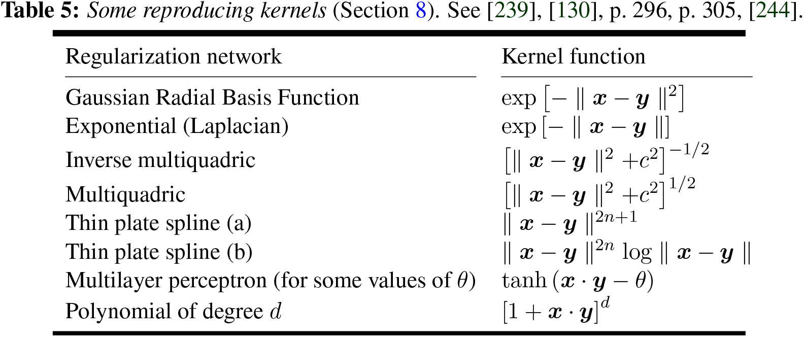
8.2 Exponential functions as reproducing kernels
A list of reproducing kernels is given in, e.g., [241] [239], such as those in Table 5. Two reproducing kernels with exponential function were used to understand how deep learning works [235], and are listed in Eq. (358): (1) the popular smooth Gaussian kernel
where σ is the standard deviation. The method in Remark 8.1 is not suitable to show that these exponential functions are reproducing kernels. We provide a verificatrion of the reproducing property of the Laplacian kernel in Eq. (358)2.
Remark 8.3. Laplacian kernel is reproducing. Consider the Laplacian kernel in Eq. (358)2 for the scalar case
The method is by using integration by parts and by using a function norm different from that in Eq. (332)2; see [240], p. 8. Now start with the integral in Eq. (332)2, and do integration by parts:
where
together with Eq. (363), and
The Kalman filter, well-known in engineering, is an example of a Gaussian-process model. See also Remark 9.6 in Section 9.5 on the 2021 US patent on Physics-Informed Learning Machine that was based on Gaussian processes (GPs),239 which possess the “most pleasant resolution imaginable” to the question of how to computationally deal with infinite-dimensional objects like functions [234], p. 2:
“If you ask only for the properties of the function at a finite number of points, then the inference from the Gaussian process will give you the same answer if you ignore the infinitely many other points, as if you would have taken them into account! And these answers are consistent with any other finite queries you may have. One of the main attractions of the Gaussian process framework is precisely that it unites a sophisticated and consistent view with computational tractability.”
A simple example of a Gaussian process is the linear model
with random coefficients
More generally,
Formally, a Gaussian process is a probability distribution over the functions
and the design matrix
Another way to put it succinctly, a Gaussian process describes a distribution over functions, and is defined as a collection of random variables (representing the values of the function
The multivariate (joint probability) Gaussian distribution for an
where
In the case of an isotropic covariance matrix
The Gaussian (normal) probability distribution
Remark 8.4. Zero mean. In a Gaussian process, the joint distribution Eq. (368) over the outputs, i.e., the
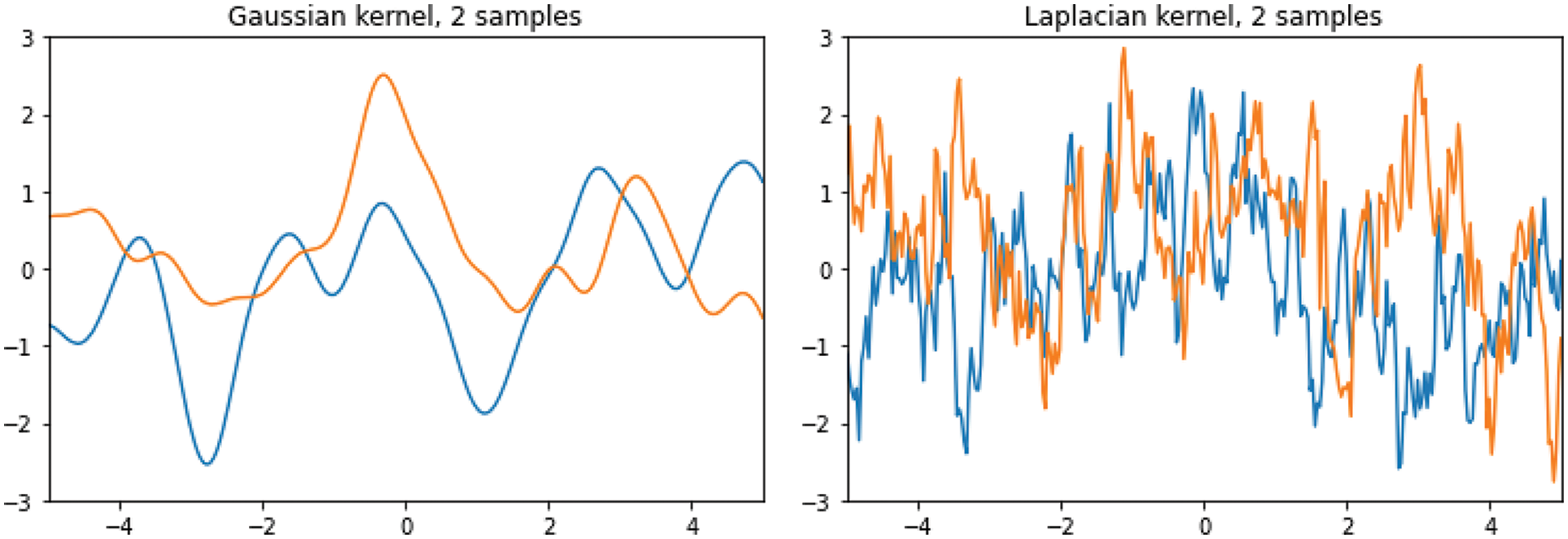
Figure 86: Gaussian process priors (Section 8.3). Left: Two samples with Gaussian kernel. Right: Two samples with Laplacian kernel. Parameters for both kernels: Kernel precision (inverse of variance)
8.3.1 Gaussian-process priors and sampling
Instead of defining the kernel function
In other words, the GP prior samples in Figure 86 were drawn from the Gaussian distribution with zero mean and covariance matrix
where
It can be observed from Figure 86 that samples obtained with the Gaussian kernel were smooth, with slow variations, whereas samples obtained with the Laplacian kernel had high jiggling with rapid variations, appropriate to model Brownian motion; see Footnote 237.
8.3.2 Gaussian-process posteriors and sampling
Let
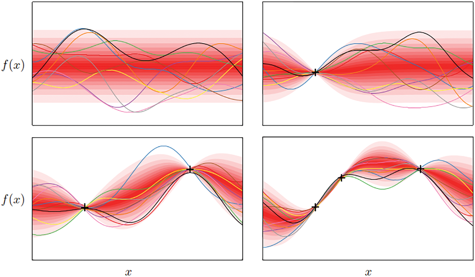
Figure 87: Gaussian process prior and posterior samplings, Gaussian kernel (Section 8.3). Top left: Gaussian-prior samples (Section 8.3.1). The shaded red zones represent the predictive density of at each input location. Top right: Gaussian-posterior samples with 1 data point. Bottom left: Gaussian-posterior samples with 2 data points. Bottom right: Gaussian-posterior samples with 3 data points [247]. See Figure 88 for the noise effects and Figure 89 for animation of GP priors and posteriors. (Figure reproduced with permission of the authors.)
The Gaussian-process posterior distribution, i.e., the conditional Gaussian distribution for the test output
where the mean was set to zero by Remark 8.4. In Figure 87, the number
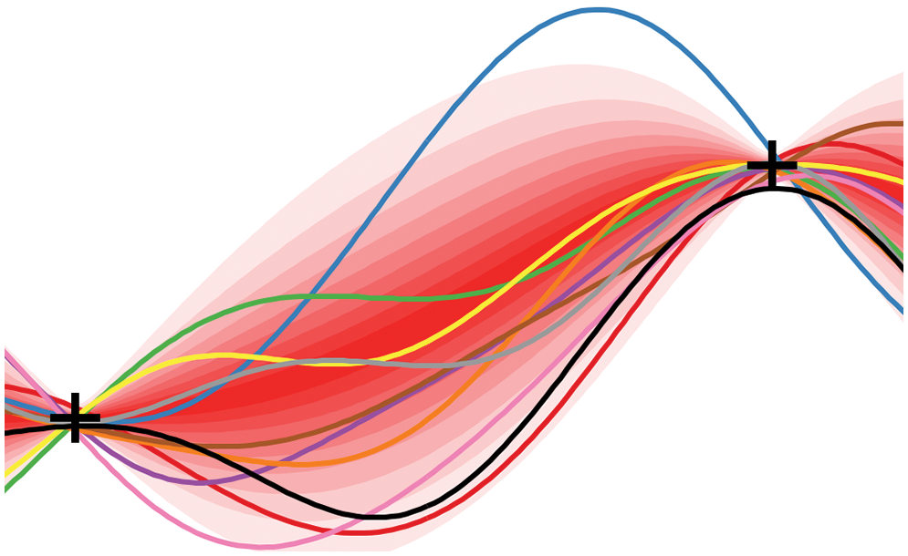
Figure 88: Gaussian process posterior samplings, noise effects (Section 8.3). Not all sampled curves in Figure 87 went through the data points, such as the black line in the present zoomed-in view of the bottom-left subfigure [247]. It is easy to make the sampled curves passing closer to the data points simply by reducing the noise variance
9 Deep-learning libraries, frameworks, platforms
Among factors that drove the resurgence of AI, see Section 2, the availability of effective computing hardware and libraries that facilitate leveraging that hardware for DL-purposes have played and continue to play an important role in terms of both expansion of research efforts and dissemination in applications. Both commercial software, but primarily open-source libraries, which are backed by major players in software industry and academia, have emerged over the last decade, see, e.g., Wikipedia’s “Comparison of deep learning software” version 12:51, 18 August 2022.
Figure 90 compares the popularity (as of 2018) of various software frameworks of the DL-realm by means of their “Power Scores”.244 The “Power Score” metric was computed from the occurrences of the respective libraries on 11 different websites, which range from scientific ones, e.g., as world’s largest storage for research articles and preprints arXiv to social media outlets as, e.g., Linkedin.
The impressive pace at which DL research and applications progress is also reflected in changes the software landscape has been subjected to. As of 2018, TensorFlow was clearly dominant, see Figure 90, whereas Theano was the only library around among those only five years earlier according to the author of the 2018 study.
As of August 2022, the picture has once again changed quite a bit. Using Google Trends as metric,245 PyTorch, which was in third place in 2018, has taken the leading position from TensorFlow as most popular DL-related software framework, see Figure 91.
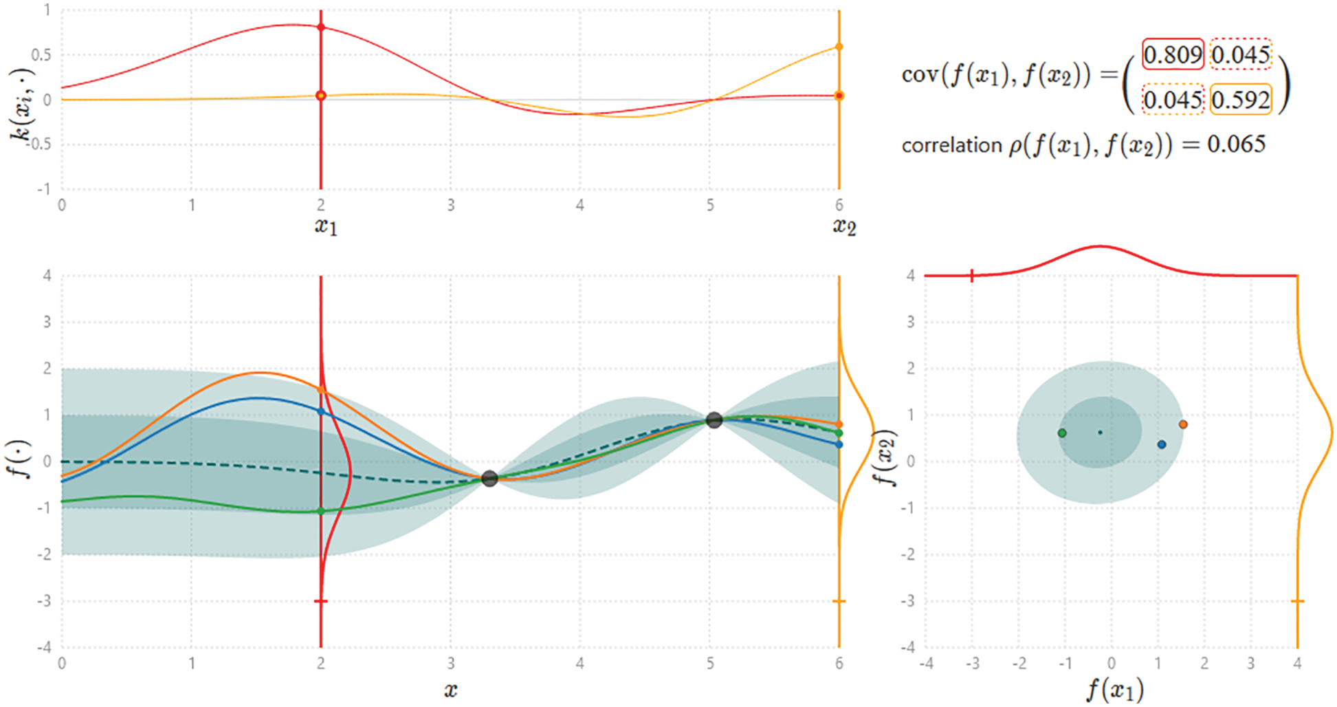
Figure 89: Gaussian process posterior samplings, animation (Section 8.3). Interactive Gaussian Process Visualization, Infinite curiosity. Click on the plot area to specify data points. See Figures 87 and 88.
Although the individual software frameworks do differ in terms of functionality, scope and internals, their overall purpose are clearly the same, i.e., to facilitate creation and training of neural networks and to harness the computational power of parallel computing hardware as, e.g., GPUs. For this reason, libraries share the following ingredients, which are essentially similar but come in different styles:
• Linear algebra: In essence, DL boils down to algebraic operations on large sets of data arranged in multi-dimensional arrays, which are supported by all software frameworks, see Section 4.4.246
• Back-propagation: Gradient-based optimization relies on efficient evaluation of derivatives of loss functions with respect to network parameters. The representation of algebraic operations as computational graphs allows for automatic differentiation, which is typically performed in reverse-mode, hence, back-propagation, see Section 5.
• Optimization: DL-libraries provide a variety of optimization algorithms that have proven effective in training of neural networks, see Section 6.
• Hardware-acceleration: Training deep neural networks is computationally intensive and requires adequate hardware, which allows algebraic computations to be performed in parallel. DL-software frameworks support various kinds of parallel/distributed hardware ranging from multi-threaded CPUs to GPUs to DL-specific hardware as TPUs. Parallelism is not restricted to algebraic computations only, but data also has to be efficiently loaded from storage and transferred to computing units.
• Frontend and API: Popular DL-frameworks provide an intuitive API, which supports accessibility for first-time learners and dissemination of novel methods to scientific fields beyond computer science. Python has become the prevailing programming language in DL, since it is more approachable for less-proficient developers as compared to languages traditionally popular in computational science as, e.g., C++ or Fortran. High-level APIs provide all essential building blocks (layers, activations, loss functions, optimizers, etc.) for both construction and training of complex network topologies and fully abstract the underlying algebraic operations from users.
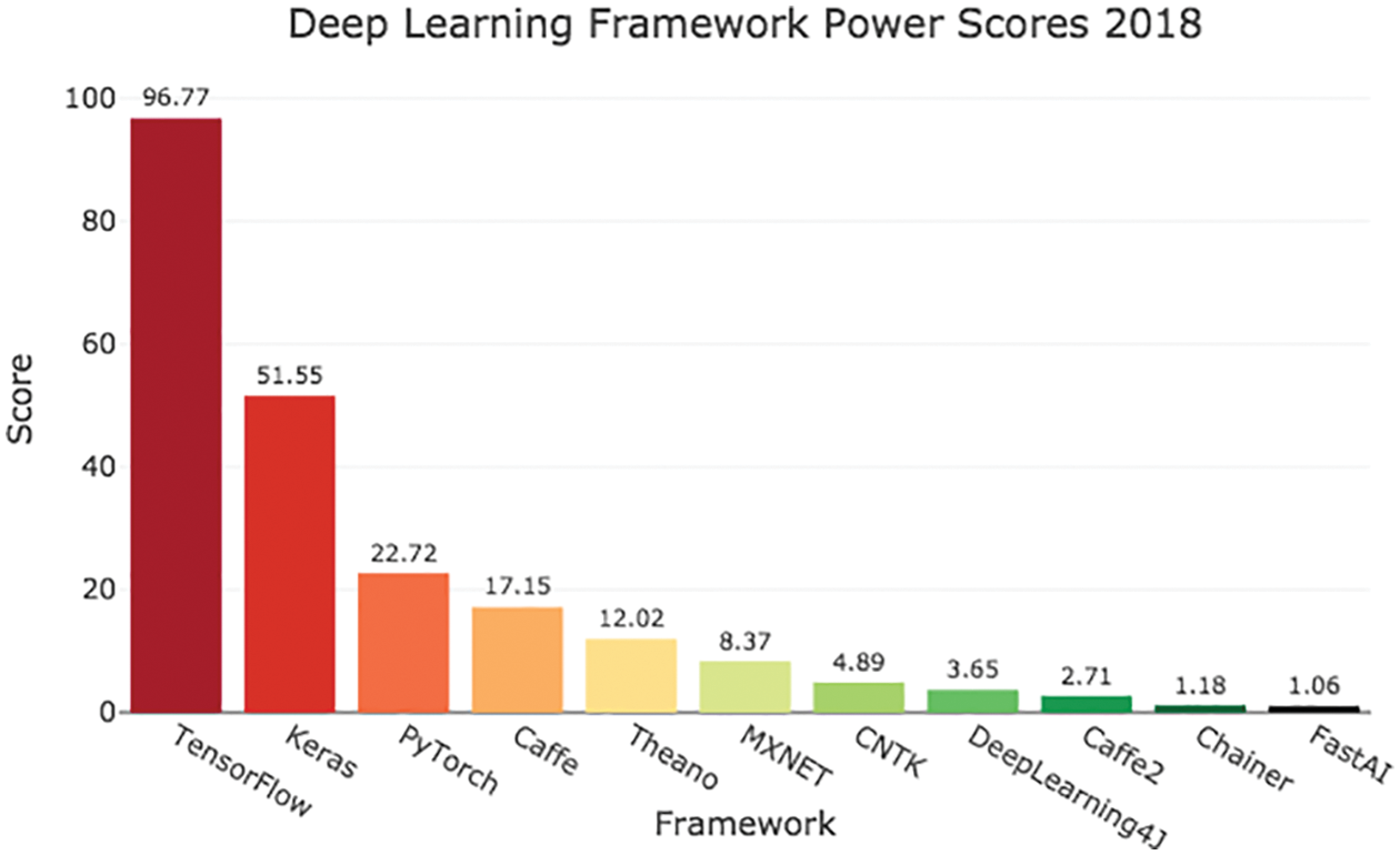
Figure 90: Top deep-learning libraries in 2018 by the “Power Score” in [249]. By 2022, using Google Trends, the popularity of different frameworks is significantly different; see Figure 91.
In what follows, a brief description of some of the most popular software frameworks is given.
TensorFlow [250] is a free and open-source software library which is being developed by the Google Brain research team, which, in turn, is part of Google’s AI division. TensorFlow emerged from Google’s proprietary predecessor “DistBelief” and was released to public in November 2015. Ever since its release, TensorFlow has rapidly become the most popular software framework in the field of deep-learning and maintains a leading position as of 2022, although it has been outgrown in popularity by its main competitor PyTorch particularly in research.
In 2016, Google presented its own AI accelerator hardware for TensorFlow called “Tensor Processing Unit” (TPU), which is built around an application-specific integrated circuited (ASIC) tailored to computations needed in training and evaluation of neural networks. DeepMind’s grandmaster-beating software AlphaGo, see Section 2.3 and Figure 2, was trained using TPUs.247 TPUs were made available to the public as part of “Google Cloud” in 2018. A single fourth-generation TPU device has a peak computing power of 275 teraflops for 16 bit floating point numbers (bfloat16) and 8 bit integers (int8). A fourth-generation cloud TPU “pod”, which comprises 4096 TPUs offers a peak computing power of 1.1 exaflops.248
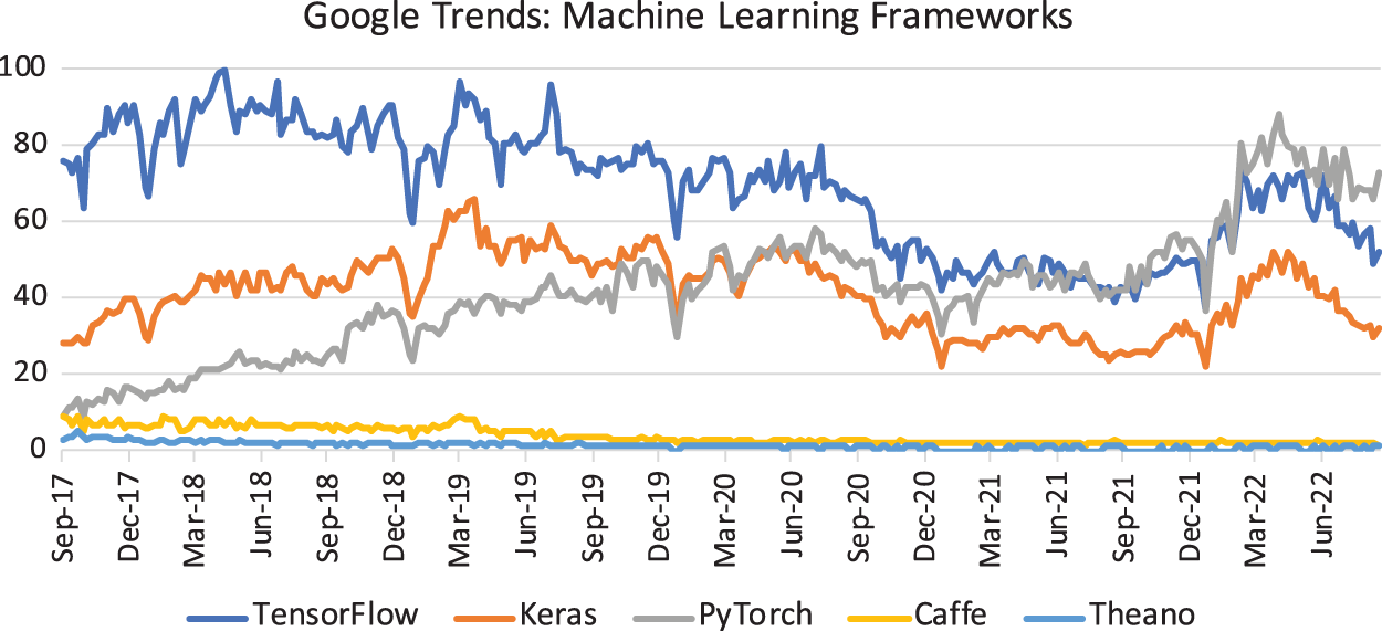
Figure 91: Google Trends of deep-learning software libraries (Section 9). The chart shows the popularity of five DL-related software libraries most “powerful” in 2018 over the last 5 years (as of July 2022). See also Figure 90 for the rankings of DL frameworks in 2018.
Keras [252] plays a special role among the software frameworks discussed here. As a matter of fact, it is not a full-featured DL-library, much rather Keras can be considered as an interface to other libraries providing a high-level API, which was originally built for various backends including TensorFlow, Theano and the (now deprecated) Microsoft Cognitive Toolkit (CNTK). As of version 2.4, TensorFlow is the only supported framework. Keras, which is free and also open-source, is meant to further simplify experimentation with neural networks as compared to TensorFlow’s lower level API.
PyTorch [253], which is a free and open-source library, which was originally released to public in January 2017.249 As of 2022, PyTorch has evolved from a research-oriented DL-framework to a fully fledged environment for both scientific work and industrial applications, which, as of 2022 has caught up with, if not surpassed, TensorFlow in popularity. Primarily addressing researchers in its early days, PyTorch saw a rapid growth not least for the–at that time–unique feature of dynamic computational graphs, which allows for great flexibility and simplifies creation of complex network architectures. As opposed to its competitors as, e.g., TensorFlow, computational graphs, which represent compositions of mathematical operations and allow for automatic differentiation of complex expressions, are created on the fly, i.e., at the very same time as operations are performed. Static graphs, on the other hand, need to be created in a first step, before they can be evaluated and automatically differentiated. Some examples of applying PyTorch to computational mechanics are provided in the next two remarks.
Remark 9.1. Reinforcement Learning (RL) is a branch of machine-learning, in which computational methods and DL-methods naturally come together. Owing to the progress in DL, reinforcement learning, which has its roots in the early days of cybernetics and machine learning, see, e.g., the survey [256], has gained attention in the fields of automatic control and robotics again. In their opening to a more recent review, the authors of [257] expect no less than “deep reinforcement-learning is poised to revolutionize artificial intelligence and represents a step toward building autonomous systems with a higher level understanding of the visual world.” RL is based on the concept that an autonomous agent learns complex tasks by trial-and-error. Interacting with its environment, the agent receives a reward if it succeeds in solving a given tasks. Not least to speed up training by means of the parallelization, simulation has become are key ingredient to modern RL, where agents are typically trained in virtual environments, i.e., simulation models of the physical world. Though (computer) games are classical benchmarks, in which DeepMind’s AlphaGo and AlphaZero models excelled humans (see Section 1, Figure 2), deep RL has proven capable of dealing with real-world applications in the field of control and robotics, see, e.g., [258]. Based on the PyTorch’s introductory tutorial (see Original website) of a the classic cart-pole problem, i.e., an inverted pendulum (pole) mounted to a moving base (cart), we developed a RL-model for the control of large-deformable beams, see Figure 92 and the video illustrating the training progress. For some large-deformable beam formulations, see, e.g., [259], [260], [261], [262]. ■
Figure 92: Positioning and pointing control of large deformable beam (Section 9, Remark 9.1). Reinforcement learning. The agent is trained to align the tip of the flexible beam with the target position (red ball). For this purpose, the agent can move the base of the cantilever; the environment returns the negative Euclidean distance of the beam’s tip to the target position as “reward” in each time-step of the simulation. Simulation video. See also GitLab repository for code and video.
JAX [263] is a free and open-source research project driven by Google. Released to the public in 2018, JAX is one of the more recent software frameworks that have emerged during the current wave of AI. It is being described as being “Autograd and XLA” and as “a language for expressing and composing transformations of numerical programs”, i.e., JAX focuses on accelerating evaluations of algebraic expression and, in particular, gradient computations. As a matter of fact, its core API, which provides a mostly NumPy-compatible interface to many mathematical operations, is rather trimmed-down in terms of DL-specific functions as compared to the broad scope of functionality offered by TensorFlow and PyTorch, for instance, which, for this reason, are often referred to as end-to-end frameworks. JAX, on the other hand, considers itself as system that facilitates “transformations” like gradient computation, just-in-time compilation and automatic vectorization of compositions of functions on parallel hardware as GPUs and TPUs. A higher-level interface to JAX’ functionality, which is specifically made for ML-purposes, is available through the FLAX framework [264]. FLAX rovides many fundamental building blocks essential for creation and training of neural networks.
9.4 Leveraging DL-frameworks for scientific computing
Software frameworks for deep-learning as, e.g., PyTorch, TensorFlow and JAX share several features which are also essential in scientific computing, in general, and finite-element analysis, in particular. These DL-frameworks are highly optimized in terms of vectorization and parallelization of algebraic operations. Within finite-element methods, parallel evaluations can be exploited in several respects: First and foremost, residual vectors and (tangent) stiffness matrices need to be repeatedly evaluated for all elements of finite-element mesh, into which the domain of interest is discretized. Secondly, the computation of each of these vectors and matrices is based upon numerical quadrature (see Section 10.3.2 for a DL-based approach to improve quadrature), which, from an algorithmic point of view, is computed as a weighted sum of integrands evaluated at a finite set of points. A further key component that proves advantages in complex FE-problems is automatic differentiation, which, in the form of backpropagation (i.e., reverse-mode automatic differentiation), is the backbone of gradient-based training of neural networks, see Section 5. In the context of FE-problems in solid mechanics, automatic differentiation saves us from deriving and implementing derivatives of potentials, whose variation and linearization with respect to (generalized) coordinates give force vectors and tangent-stiffness matrices.250
The potential of modern DL-software frameworks in conventional finite-element problems was studied in [266], where Netgen/NGSolve, which is a highly-optimized, OpenMP-parallel finite-element code written in C++, was compared against PyTorch and JAX implementations. In particular, the computational efficiency of the computing and assembling vectors of internal forces and tangent stiffness matrices of a hyperelastic solid was investigated. On the same (virtual) machine, it turned out that both PyTorch and JAX can compete with Netgen/NGSolve when computations are performed on CPU, see the timings shown in Figure 93. Moving computations to a GPU, the Python-based DL-frameworks outperformed Netgen/NGSolve in the evaluation of residual vectors. Regarding tangent-stiffness matrices, which are obtained through (automatic) second derivatives of the strain-energy function with respect to nodal coordinates, both PyTorch and JAX showed (different) bottlenecks, which, however, are likely to be sorted out in future releases.
9.5 Physics-Informed Neural Network (PINN) frameworks
In laying out the roadmap for “Simulation Intelligence” (SI) the authors of [267] considered PINN as a key player in the first of the nine SI “motifs,” called “Multi-physics & multi-scale modeling.”
The PINN method to solve differential equations (ODEs, PDEs) aims at training a neural network to minimize the total weighted loss
where
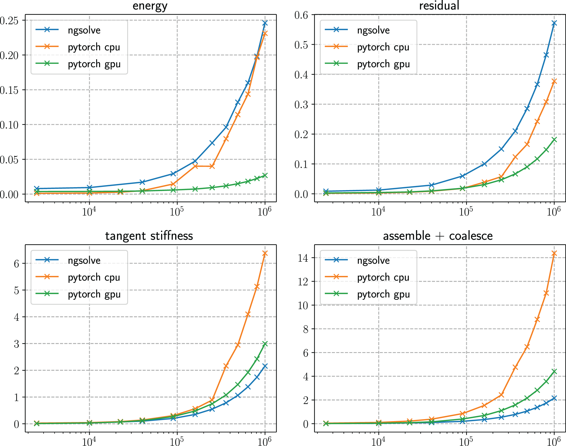
Figure 93: DL-frameworks in nonlinear finite-element problems (Section 9.4). The computational efficiency of a PyTorch-based (Version 1.8) finite-element code implemented was compared against the state-of-the-art general purpose Netgen/NGSolve [265] for a problem of nonlinear elasticity, see the slides of the presentation and the corresponding video. The figures show timings (in seconds) for evaluations of the strain energy (top left), the internal forces (residual, top right) and element-stiffness matrices (bottom left) and the global stiffness matrix (bottom right) against the number of elements. Owing to PyTorch’s parallel computation capacity, the simple Python implementation could compete with the highly-optimized finite-element code, in particular, as computations were moved to a GPU (NVIDIA Tesla V100).
Some review papers on PINN are [269] [270], with the latter being more general than [268], which was restricted to fluid mechanics, and touching on many different fields. Table 6 lists PINN frameworks that are currently actively developed, and a few selected solvers among which are summarized below.
☛ DeepXDE [271], one of the first PINN framework and a solver (Table 6) was developed in Python, with a TensorFlow backend, for both teaching and research. This framework can solve both forward problems (“given initial and boundary conditions”) and inverse problems (“given some extra measures”), with domains having complex geometry. According to the authors, DeepXDE is user-friendly, with compact user code resembling the problem mathematical formulation, customizable to different types of mechanics problem. The site contains many published papers with a large number of demo problems: Poisson equation, Burgers equation, diffusion-reaction equation, wave propagation equation, fractional PDEs, etc. In addition, there are demos on inverse problems and operator learning. Three more backends beyond TensorFlow, which was reported in [270], have been added to DeepXDE: PyTorch, JAX, Paddle.252
☛ NeuroDiffEq [274], a solver, was developed about the same time as DeepXDE, with the backend being PyTorch. Even though it was written that the authors were “actively working on extending NeuroDiffEq to support three spatial dimensions,” this feature is not ready, and can be worked around by including the 3D boundary conditions in the loss function.253 Even though in principle, NeuroDiffEq can be used to solve PDEs of interest to engineering (e.g., Navier-Stokes solutions), there were no such examples in the official documentation, except for a 2D Laplace equation and a 1D heat equation. The backend is limited to PyTorch, and the site did not list any papers, either by the developers or by others, using this framework.
☛ NeuralPDE [275], a solver, was developed in a relatively new language Julia, which is 20 years younger than Python, has a speed edge over Python in machine learning, but does not in data science.254 Demos are given for ODEs, generic PDEs, such as the coupled nonlinear hyperbolic PDEs of the form:
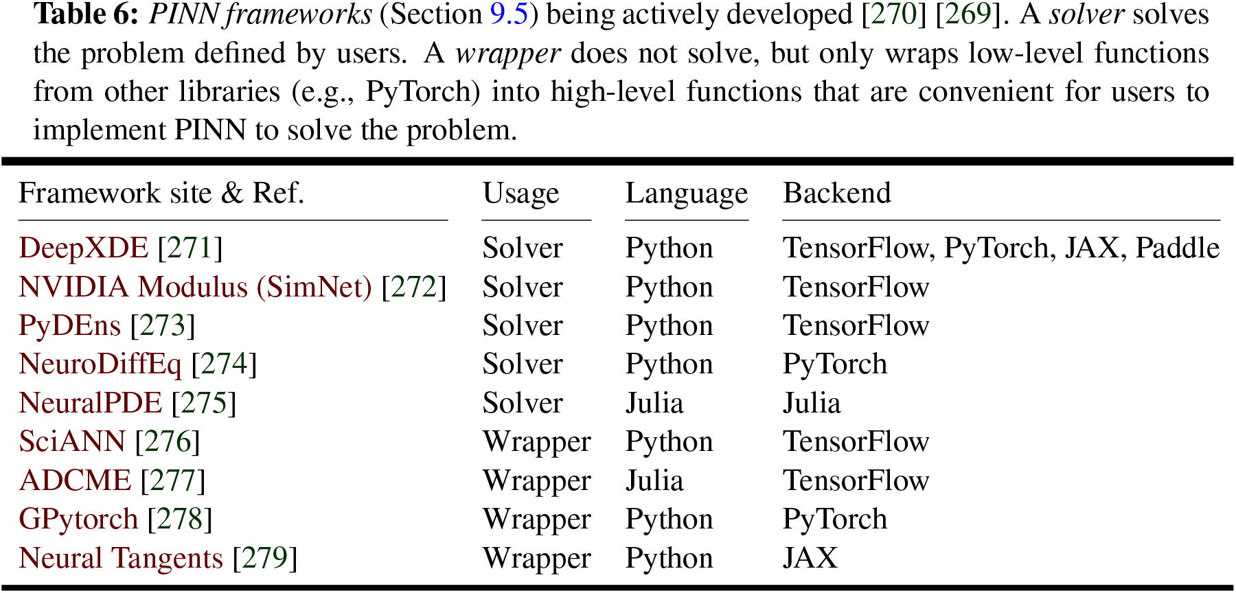
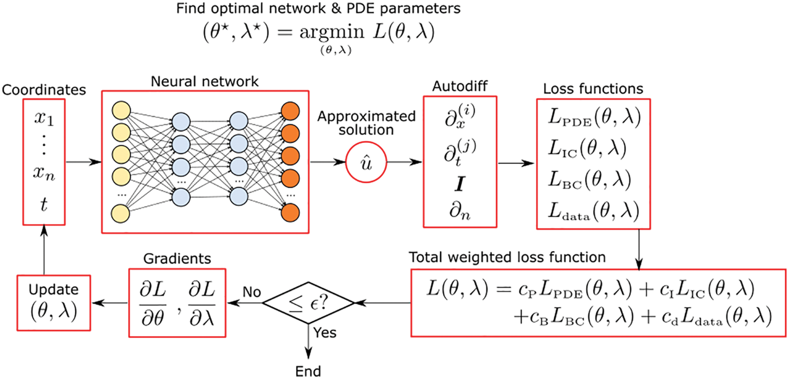
Figure 94: Physics-Informed Neural Networks (PINN) concept (Section 9.5). The goal is to find the optimal network parameters
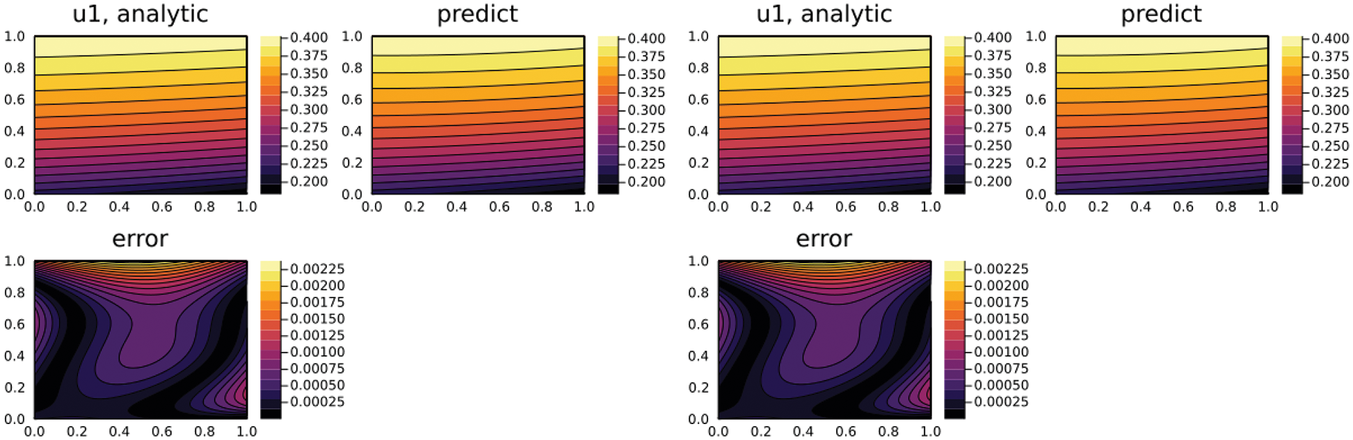
Figure 95: Coupled nonlinear hyperbolic equations (Section 9.5). Analytical solution, predicted solution by NeuralPDE [275] and error for the coupled nonlinear hyperbolic equations in Eq. (383).
with
Additional PINN software packages other than those in Table 6 are listed and summarized in [269].
Remark 9.2. PINN and activation functions. Deep neural networks (DNN), having at least two hidden layers, with ReLU activation function (Figure 24) were shown to correspond to linear finite element interpolation [280], since piecewise linear functions can be written as DNN with ReLU activation functions [281].
But using the strong form such as the PDE in Eq. (383), which has the second partial derivative with respect to
for which the hyperbolic tangent (
Remark 9.3. Variational PINN. Similar to the finite element method, in which the weak form, not the strong form as in Remark 9.2, of the PDE allows for a reduction in the requirement of differentiability of the trial solution, and is discretized with numerical integration used to evaluate the resulting coefficients for various matrices (e.g, mass, stiffness, etc), PINN can be formulated using the weak form, instead of the strong form such as Eq. (385), at the expense of having to perform numerical integration (quadrature) [283] [284] [285].
Examples of 1-D PDEs were given in [283] in which the activation function was a sine function defined over the interval
where
where the familiar symmetric operator A2 in Eq. (389) is the weak form, with the non-symmetric operator A1 in Eq. (388) retaining the second derivation on the solution
which does not satisfy the essential boundary conditions (whereas the solution
where
For a symmetric variational form such as
which is similar to the approach taken in [280], where the ReLU activation function (Figure 24) was used, and where a constraint on the NN parameters was used to satisfy an essential boundary condition. ■
Remark 9.4. PINN, kernel machines, training, convergence problems. There is a relationship between PINN and kernel machines in Section 8. Specifically, the neural tangent kernel [232], which “captures the behavior of fully-connected neural networks in the infinite width limit during training via gradient descent” was used to understand when and why PINN failed to train [286], whose authors found a “remarkable discrepancy in the convergence rate of the different loss components contributing to the total training error,” and proposed a new gradient descent algorithm to fix the problem.
It was often reported that PINN optimization converged to “solutions that lacked physical behaviors,” and “reduced-domain methods improved convergence behavior of PINNs”; see [287], where a dynamical system of the form below was studied:
with
See also [288] for incorporating the Lyapunov stability concept into PINN formulation for CFD to “improve the generalization error and reduce the prediction uncertainty.” ■
Remark 9.5. PINN and attention architecture. In [228], PIANN, Physics-Informed Attention-based Neural Network, was proposed to connect PINN to attention architecture, discussed in Section 7.4.3 to solve hyperbolic PDE with shock wave. See Remark 7.7 and Remark 11.11. ■
Remark 9.6. “Physics-Informed Learning Machine” (PILM) 2021 US Patent [289]. First note that the patent title used the phrase “learning machine,” instead of “machine learning,” indicating that the emphasis of the patent appeared to be on “machine,” instead of on “learning” [289]. PINN was not mentioned, as it was first invented in [290] [291], which were cited by the patent authors in their original PINN paper [282].255 The abstract of this 2021 PILM US Patent [289] reads as follows:
“A method for analyzing an object includes modeling the object with a differential equation, such as a linear partial differential equation (PDE), and sampling data associated with the differential equation. The method uses a probability distribution device to obtain the solution to the differential equation. The method eliminates use of discretization of the differential equation.”
The first sentence is nothing new to the readers. In the second sentence, a “probability distribution device” could be replaced by a neural network, which would make PILM into PINN. This patent mainly focused on the Gaussian processes (Section 8.3), as an exemple of probability distribution (see Figure 4 in [289]). The third sentence would be the claim-to-fame of PILM, and also of PINN. ■
Remark 9.7. Using PINN frameworks. While undergraduates with limited knowledge on the theory of the Finite Element Method could run FE Analysis of complicated structures and complex domain geometries on a laptop using commercial FE codes, solving problems with exceedingly simple domain geometry using a PINN framework such as DeepXDE does require knowledge of governing PDEs, initial and boundary conditions, artificial neural networks and frameworks (such as PyTorch, TensorFlow, etc.), the Python language, and having a more powerful computer. In addition, because there are many parameters to fiddle with, beyond the sample problems posted on the DeepXDE website, first-time users could encounter disappointment and doubt when trying to solve a new problem. It is not clear when the PINN methods would reach the level of FE commercial codes that undergraduates could use, or would they just fade away after an initial period of excitement like the meshless methods before them. ■
10 Application 1: Enhanced numerical quadrature for finite elements
The results and deep-learning concepts used in [38] were presented in Section 2.3.1 above. In this section, we discuss some details of the formulation.
The finite element method (FEM) has become the most important numerical method for the approximation of solutions to partial differential equations, in particular, the governing equations in solid mechanics. As for any mesh-based method, the discretization of a continuous (spatial, temporal) domain into a finite-element mesh, i.e., a disjoint set of finite elements, is a vital ingredient that affects the quality of the results and therefore has emerged as a field of research on its own. Being based on the weak formulation of the governing balance equations, numerical integration is a second key ingredient of FEM, in which integrals over the physical domain of interest are approximated by the sum of integrals over the individual finite elements. In real-world problems, regularly shaped elements, e.g., triangles and rectangles in 2-D, tetrahedra and hexahedra in 3-D, typically no longer suffice to represent the complex shape of bodies or physical domains. By distorting basic element shapes, finite elements of more arbitrary shapes are obtained, while the interpolation functions of the “parent” elements can be retained.256 The mapping represents a coordinate transformation by which the coordinates of a “parent” or “reference” element are mapped onto distorted, possibly curvilinear, physical coordinates of the actual elements in the mesh. Conventional finite element formulations use polynomials as interpolation functions, for which Gauss-Legendre quadrature is the most efficient way to integrate numerically. Efficiency in numerical quadrature is immediately related the (finite) number of integration points that is required to exactly integrate a polynomial of a given degree.257 For distorted elements, the Jacobian of the transformation describing the distortion of the parent element renders the integrand of, e.g., the element stiffness matrix non-polynomial. Therefore, the integrals generally are not integrated exactly using Gauss-Legendre quadrature, but the accuracy depends, roughly speaking, on the degree of distortion.
10.1 Two methods of quadrature, 1-D example
To motivate their approaches, the authors of [38] presented an illustrative 1-D example of a simple integral, which was analytically integrated as
Using 2 integration points, Gauss-Legendre quadrature yields significant error
which is owed to the insufficient number of integration points.
Method 1 to improve accuracy, which is reflected in Application 1.1 (see Section 10.2), is to increase the number of integration points. In the above example, 6 integration points are required to obtain the exact value of the integral. By increasing the accuracy, however, we sacrifice computational efficiency due the need for 6 evaluations of the integrand instead of the original 2 evaluations.
Method 2 is to retain 2 integration points, and to adjust the quadrature weights at the integration points instead. If the same quadrature weights of
By adjusting the quadrature weights rather than the number of integration points, which is the key concept of Application 1.2 (see Section 10.3), the computational efficiency of the original approach Eq. (398) is retained.
In this study [38], hexahedral elements with linear shape functions were considered. To exactly integrate the element stiffness matrix of an undistorted element
To train the neural networks involved in their approaches, a large set of distorted elements was created by randomly displacing seven nodes of a regular cube [38],
where
Figure 96: Normalization procedure for hexahedra (Section 10.1). Numerical integration is performed in local element coordinates. The accuracy of Gauss-Legendre quadrature only depends on the element shape, i.e., it is invariant with respect to rigid-body motion and uniform stretching deformation. For this reason, a normalization procedure was introduced involving one translation and three rotations (second from left to right) for linear hexahedral elements, whose nodes are labelled as shown for the regular hexahedron (left) [38]. (1) The element is displaced such that node A coincides with the origin O of the global frame. (2) The hexahedron is rotated about the z-axis of the global frame to place node B in the xz-plane, and then (3) rotated about the y-axis such that node B lies on the x-axis. (4) A third rotation about the x-axis relocates node D to the xy-plane of the global frame. (5) Finally (not shown), the element is scaled by a factor of
To quantify the quadrature error, the authors of [38] introduced
where
10.2 Application 1.1: Method 1, Optimal number of integration points
The details of this particular deep-learning application, mentioned briefly in Section 2.3 on motivation via applications of deep learning–specifically Section 2.3.1, item (1)–are provided here. The idea is to have a neural network predict, for each element (particularly distorted elements), the number of integration points that provides accurate integration within a given error tolerance
10.2.1 Method 1, feasibility study
In the example in [38], the quadrature error is required to be smaller than
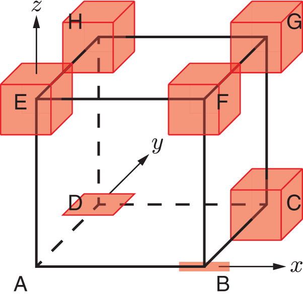
Figure 97: Creation of randomly distorted elements (Section 10). Hexahedra forming the training and validation sets are created by randomly displacing the nodes of a regular hexahedral. To comply with the normalization procedure, node A remains fixed, node B is shifted along the
10.2.2 Method 1, training phase
To train the network, 2000 randomly distorted elements were generated for each of the five degrees of maximum distortion,
The whole dataset was partitioned262 into a training set
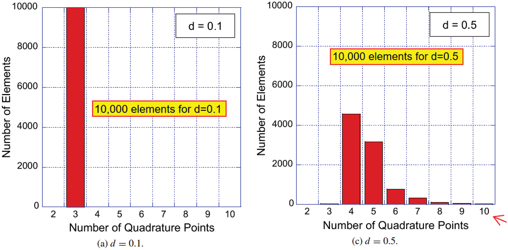
Figure 98: Method 1, Optimal number of integration points, feasibility (Section 10.2.1). Distribution of minimum numbers of integration points on a local coordinate axes for a maximum error of etol = 10−3 among 10,000 elements generated randomly using the method in Figure 97. For d = 0:1, all elements were only slightly distorted, and required 3 integration points each. For d = 0:5, close to 5,000 elements required 4 integration points each; very few elements required 3 or 10 integration points [38]. (Figure reproduced with permission of the authors.)
10.2.3 Method 1, application phase
The correct number of quadrature points and the corresponding number of points predicted by the neural network are illustrated in Figure 100 for both the training set (“patterns”) in Table (a) and the validation set (“test patterns”) in Table (b).
Both the training set and the validation set, each had 5000 distorted element shapes. As an example to interpret these tables, take Table (a), Row 2 (red underline, labeled “3” in red circle) of the matrix (blue box): Out of a Total of 1562 element shapes (last column) in the training set that were ideally integrated using 3 quadrature points (in red circle), the neural network correctly estimated a need of 3 quadrature points (Column 2, labeled “3” in red circle) for 1553 element shapes, and 4 quadrature points (Column 3, labeled “4” in red circle) for 9 element shapes. That’s an accuracy of 99.4% for Row 2. The accuracy varies, however, by row, 0% for Row 1 (2 integration points), 99.6% for Row 3,..., 71.4% for Row 7, 0% for Row 8 (9 integration points). The numbers in column “Total” add up to 5 + 1562 + 2557 + 636 + 162 + 55 + 21 + 2 = 5000 elements in the training set. The diagonal coefficients add up to 1553 + 2548 + 616 + 153 + 46 + 15 = 4931 elements with correctly predicted number of integration points, yielding the overall accuracy of 4931 / 5000 = 98.6% in training, Figure 99.
Figure 99: Method 1, Optimal network architecture for training (Section 10.2.2). The number of hidden layers varies from 1 to 5, keeping the number of neurons per hidden layer constant at 50. The network with 3 hidden layers provided the highest accuracy for both the training set (“patterns”) at 98.6% and for the validation set (“test patterns”) at 81.6%. Increase the network depth does not necessarily increase the accuracy [38]. (Table reproduced with permission of the authors.)
For Table (b) in Figure 100, the numbers in column “Total” add up to 5 + 1553 + 2574 + 656 + 135 + 56 + 21 + 5 = 5005 elements in the validation set, which should have 5000, as written by [38]. Was there a misprint ? The diagonal coefficients add up to 1430 + 2222 + 386 + 36 + 6 = 4080 elements with correctly predicted number of integration points, yielding the accuracy of 4080 / 5000 = 81.6%, which agrees with Row 3 in Figure 99. As a result of this agreement, the number of elements in the validation set (“test patterns”) should be 5000, and not 5005, i.e., there was a misprint in column “Total”.
10.3 Application 1.2: Method 2, optimal quadrature weights
The details of this particular deep-learning application, mentioned briefly in Section 2.3 on motivation via applications of deep learning, Section 2.3.1, item (2), are provided here. As an alternative to increasing the number of quadrature points, the authors of [38] proposed to compensate for the quadrature error introduced by the element distortion by adjusting the quadrature weights at a fixed number of quadrature points. For this purpose, they introduced correction factors
The data preparation here was similar to that in Method 1, Section 10.2, except that 20,000 randomly distorted elements were generated, with 4000 elements in each of the five groups, each group having a different degree of maximum distortion
10.3.1 Method 2, feasibility study
Using the above 20,000 elements, the feasibility of improving integration accuracy by quadrature weight correction was established in Figure 101. To obtain these results, a brute-force search was used: For each of the 20000 elements, 1 million sets of random correction factors
i.e., the ratio between the quadrature error defined in Eq. (401) obtained using the optimal (“opt”) corrected quadrature weights and the quadrature error obtained using the standard quadrature weights of Gauss-Legendre quadrature. Accordingly, a ratio
Figure 100: Method 1, application phase (Section 10.2.3). The numbers of quadrature points predicted by the neural network was compared to the minimum numbers of quadrature points for maximum error
were retained as target values for training, and identified with the superscript “opt”, standing for “optimal”. The corresponding optimally integrated coefficients in the element stiffness matrix are denoted by
It turns out that a reduction of the quadrature error by correcting the quadrature weights is not feasible for all element shapes. Undistorted elements, for instance, which are already integrated exactly using standard quadrature weights, naturally do not admit improvements. These 20,000 elements were classified into two categories A and B [38], Figure 101. Quadrature weight correction was not effective for Category A (
10.3.2 Method 2, training phase
Because the effectiveness of the quadrature weight correction strongly depends on the degree of maximum distortion,
In the first stage, a first neural network, a binary classifier, was trained to predict whether an element shape admits improved accuracy by quadrature weight correction (Category B) or not (Category A). The neural network to perform the classification task took the 18 non-trivial nodal coordinates obtained upon the proposed normalization procedure for linear hexahedra as inputs, i.e.,
Figure 101: Method 2, Quadrature weight correction, feasibility (Section 10.3.1). Each element was tested 1 million times with randomly generated sets of quadrature weights. There were 4000 elements in each of the 5 groups with different degrees of maximum distortion,
Out of the 20000 elements generated, 10000 elements were selected to train the classifier network, for which both the training set and the validation set comprised 5000 elements each [38].266 The optimal neural network in terms of classification accuracy for this application had 4 hidden layers with 30 neurons per layer; see Figure 102. The trained neural network succeeded in predicting the correct category for 98 %, & 92 % of the elements in the training set and in the validation set, respectively.
In the second stage, a second neural network was trained to predict the corrections to the quadrature weights for all those elements, which allowed a reduction of the quadrature error. Again, the 18 non-trivial nodal coordinates of a normalized hexahedron were input to the neural network, i.e.,
10.3.3 Method 2, application phase
The effectiveness of the numerical quadrature with corrected quadrature weights was already presented in Figure 10 in Section 2.3.1, with the distribution of the error-reduction ratio
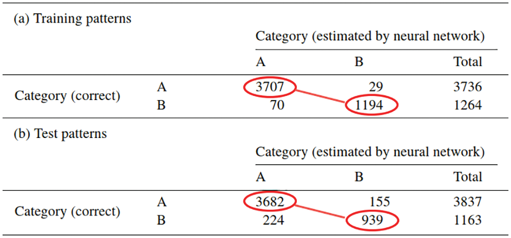
Figure 102: Method 2, training phase, classifier network (Section 10.3.2). The training and validation sets comprised 5000 elements each, of which 3707 and 3682, respectively, belonged to Category A (no improvements upon weight correction). A first neural network with 4 hidden layers of 30 neurons correctly classified
The red bars (“Optimized”) in Figure 10 represent the distribution of the error-reduction ratio
The blue bars (“Estimated by Neuro”) correspond to the error reduction ratios achieved with the corrected quadrature weights that were predicted by the trained neural network.
The error-reduction ratios
There were no red bars (optimal weights) with
The authors of [38] concluded their paper with a discussion on the computational efforts, and in particular the evaluation of trained neural networks in the application phase. As opposed to computational mechanics, where we are used to double precision floating-point arithmetics, deep neural networks have proven to perform well with reduced numerical precision.270 To speed up the evaluation of the trained networks, the least significant bits from all parameters (weights, biases) and the inputs were simply removed [38]. In both the estimation of the number of quadrature points and the prediction of the weight correction factors, half precision floating-point numbers (16 bit) turn out to show sufficient accuracy almost on par with single precision floats (32 bit).
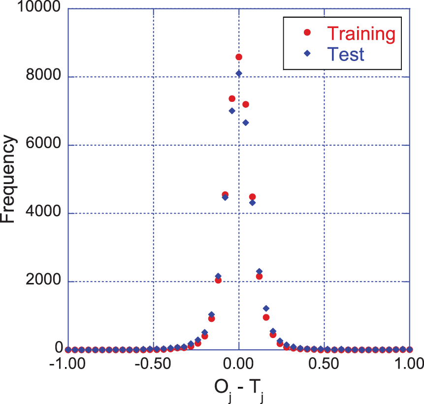
Figure 103: Method 2, training phase, regression network (Section 10.3.2). A second neural network estimated 8 correction factors
11 Application 2: Solid mechanics, multi-scale, multi-physics
The results and deep-learning concepts used in [25] were presented in Section 2.3.2 further above. In this section, we discuss some details of the formulation.
Multiscale problems are characterized by the fact that couplings of physical processes occurring on different scales of length and/or time needs to be considered. In the field of computational mechanics, multiscale models are often used to accurately capture the constitutive behavior on a macroscopic length scale, since resolving the entire domain under consideration on the smallest relevant scale if often intractable. To reduce the computational costs, multiscale techniques as, e.g., coupled DEM-FEM or coupled FEM-FEM (known as FEM
The multiscale problem in the mechanics of porous media tackled in [25] is represented in Figure 104, where the relative orientations among the three models at microscale, mesoscale, and macroscale in Figure 14 are indicated. The method of analysis (DEM or FEM) in each scale is also indicated in the figure.
11.2 Data-driven constitutive modeling, deep learning
Despite the diverse approaches proposed, multiscale problems remain a computationally challenging task, which was tackled in [25] by means of a hybrid data-driven method by combining deep neural networks and conventional constitutive models. To illustrate the hierarchy among the relations of models and to identify, the authors of [25] used directed graphs, which also indicated the nature of the individual relations by the colors of the graph edges. Black edges correspond to “universal principles” whereas red edges represent phenomenological relations, see, e.g., the classical problem in solid mechanics shown in Figure 105. Within classical mechanics, the balance of linear momentum is axiomatic in nature, i.e., it represents a well-accepted premise that is taken to be true. The relation between the displacement field and the strain tensor represents a definition. The constitutive law describing the stress response, which, in the elastic case, is an algebraic relation among stresses and strains, is the only phenomenological part in the “single-physics” solid mechanics problem and, therefore, highlighted in red.
Figure 104: Three scales in data-driven fault-reactivation simulations (Sections 2.3.2, 11.1, 11.3.5). Relative orientation of Representative Volume Elements (RVEs). Left: Microscale (

Figure 105: Single-physics block diagram (Section 11.2). Single physics is an easiest way to see the role of deep learning in modeling complex nonlinear constitutive behavior (stress-strain relation, red arrow), as first realized in [23], where balance of linear momentum and strain-displacement relation are definitions or accepted “universal principles” (black arrows) [25]. (Figure reproduced with permission of the authors.)
In many engineering problems, stress-strain relations of, possibly nonlinear, elasticity, which are parameterized by a set of elastic moduli, can be used in the modeling. For heterogeneous materials as, e.g., in composite structures, even the “single physics” problem of elastic solid mechanics may necessitate multiscale approaches, in which constitutive laws are replaced by RVE simulations and homogenization. This approach was extended to multiphysics models of porous media, in which multiple scales needed to be considered [25]. The counterpart of Figure 105 for the mechanics of porous media is complex, could be confusing for readers not familiar with the field, does not add much to the understanding of the use of deep learning in this study, and therefore not included here; see [25].
The hybrid approach in [25], which was described as graph-based machine learning model, retained those parts of the model which represented universal principles or definitions (black arrows). Phenomenological relations (red arrows), which, in conventional multiscale approaches, followed from microscale models, were replaced by computationally efficient data-driven models. In view of the path-dependency of the constitutive behavior in the poromechanics problem considered, it was proposed in [25] to use recurrent neural networks (RNNs), Section 7.1, constructed with Long Short-Term Memory (LSTM) cells, Section 7.2.
11.3 Multiscale multiphysics problem: Porous media
The problem of hydro-mechanical coupling in deformable porous media with multiple permeabilities is characterized by the presence of two or more pore systems with different typical sizes or geometrical features of the host matrix [25]. The individual pore systems may exchange fluid depending on whether the pores are connected or not. If the (macroscopic) deformation of the solid skeleton is large, plastic deformation and cracks may occur, which result in anisotropic evolution of the effective permeability. As a consequence, problems of this kind are not characterized by a single effective permeability, and, to identify the material parameters on the macroscopic scale, micro-structural models need to be incorporated.
The authors of [25] considered a saturated porous medium, which features two dominant pore scales: The regular solid matrix was characterized by micropores, whereas macropores may result, e.g., from cracks and fissures. Both the volume and the partial densities of each constituent in the mixture of solid, micropores, macropores and voids were characterized by the porosity, i.e., the (local) ratio of pores and the total volume, as well as the fractions of the respective pore systems.
11.3.1 Recurrent neural networks for scale bridging
Recurrent neural networks (RNNs, Section 7.1), which are equivalent to “very deep feedforward networks” (Remark 7.2), were used in [25] as a scale-bridging method to efficiently simulate multiscale problems of poroplasticity. In Figure 14, Section 2.3.2, three scales were considered: Microscale (
At the microscale, Discrete Element Method (DEM) is used to simulate a mesoscale Representative Volume Element (RVE) that consists of a cubic pack of microscale particles, with different loading conditions to generate a training set for a mesoscale RNN with LSTM architecture to model mesoscale constitutive response to produce loading histories
At the mesocale, Finite Element Method (FEM), combined with mesoscale loading histories
At the macroscale, Finite Element Method (FEM), combined with macroscale loading histories
11.3.2 Microstructure and principal direction data
To train the mesoscale RNN with LSTM units (which was called the “Mesoscale data-driven constitutive model” in [25]), incorporating microstucture data–such as the fabric tensor
Figure 106: Microscale RVE (Sections 11.3.2, 11.3.3, 11.3.5). A
where
Remark 11.1. Even though in Figure 14 (row 1) in Section 2.3.2, the microscale RVE was indicated to be of micron size, but the microscale RVE in Figure 106 was of size
Other microstructure data such as the porosity and the coordination number (or number of contact point), being scalars and did not incorporate directional data like the fabric tensor, did not help to improve the accuracy of the network prediction, as noted in the caption of Figure 17.
To enforce objectivity of constitutive models realized as neural networks, (the history of) principal strains and incremental rotation parameters that describe the orientation of principal directions served as inputs to the network. Accordingly, principal stresses and incremental rotations for the principal directions were outputs of what was referred to as Spectral RNNs [25], which preserved objectivity of constitutive models.
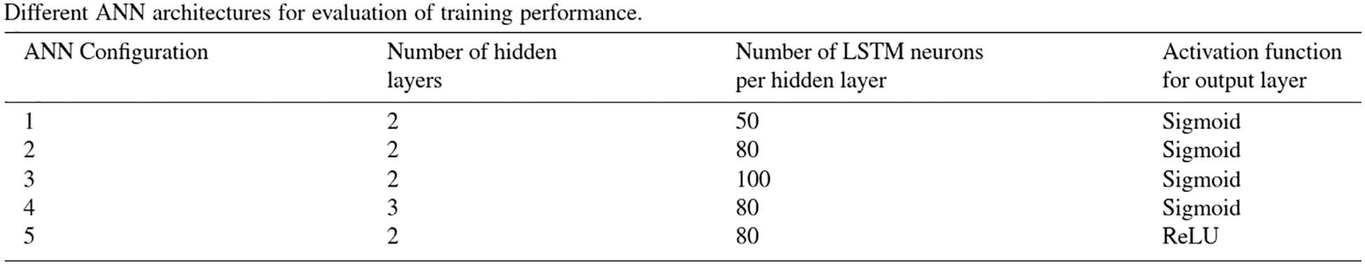
Figure 107: Optimal RNN-LSTM architecture (Section 11.3.3). 5 different configurations of RNNs with LSTM units [25]. (Table reproduced with permission of the authors.)
11.3.3 Optimal RNN-LSTM architecture
Using the same discrete element assembly of microscale RVE in Figure 106 to generate data, the authors of [25] tried out 5 different configurations of RNNs with LSTM units, with 2 or 3 hidden layers, 50 to 100 LSTM units (Figure 15, Section 2.3.2, and Figure 81 for the detailed original LSTM cell), and either logistic sigmoid or ReLU as activation function, Figure 107.
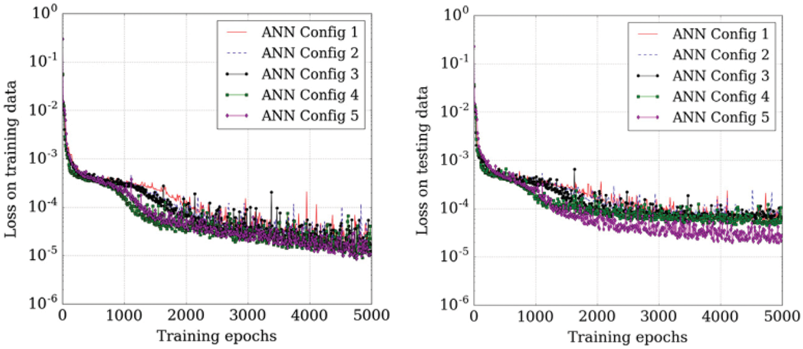
Figure 108: Optimal RNN-LSTM architecture (Section 11.3.3). Training error and test errors for 5 different configurations of RNN with LSTM units, see Figure 107 [25] (Figure reproduced with permission of the authors.)
Configuration 1 has 2 hidden layers with 50 LSTM units each, and with the logistic sigmoid as activation function. Config 2 is similar, but with 80 LSTM units per hidden layer. Config 3 is similar, but with 100 LSTM units per hidden layer. Config 4 is similar to Config 2, but with 3 hidden layers. Config 5 is similar to Config 4, but with ReLU activation function.
The training error and test error obtained from using these 5 configurations are shown in Figure 108. The zoomed-in views of the training error and test error from epoch 3000 to epoch 5000 in Figure 109 show that Config 5 was the optimal with smaller errors, and since ReLU would be computationally more efficient than the logistic sigmoid. But Config 2 was, however, selected in [25], whose authors cited that the discrepancy was “not significant”, and that Config 2 gave “good training and prediction performances”.
Remark 11.2. The above search for an optimal network architecture is similar to searching for an appropriate degree of a polynomial function for a best fit, avoiding overfit and underfit, over a given set of data points in a least-square curve fittings. See Figure 72 in Section 6.5.9 for an explanation of underfit and overfit, and Figure 99 in Section 10 for a similar search of an optimal network for numerical integration by ANN. ■
Remark 11.3. Referring to Remark 4.3 and the neural network in Figure 14 and to our definition of action depth as total number of action layers
Remark 11.4. The same selected architecture of RNN with LSTM units on both the microscale RVE (Figure 106, Figure 110) and the mesoscale RVE (Figure 112, Figure 113) was used to produce the mesoscale RNN with LSTM units (“Mesoscale data-driven constitutive model”) and the macroscale RNN with LSTM units (“Macroscale data-driven constitutive model”), respectively [25]. ■
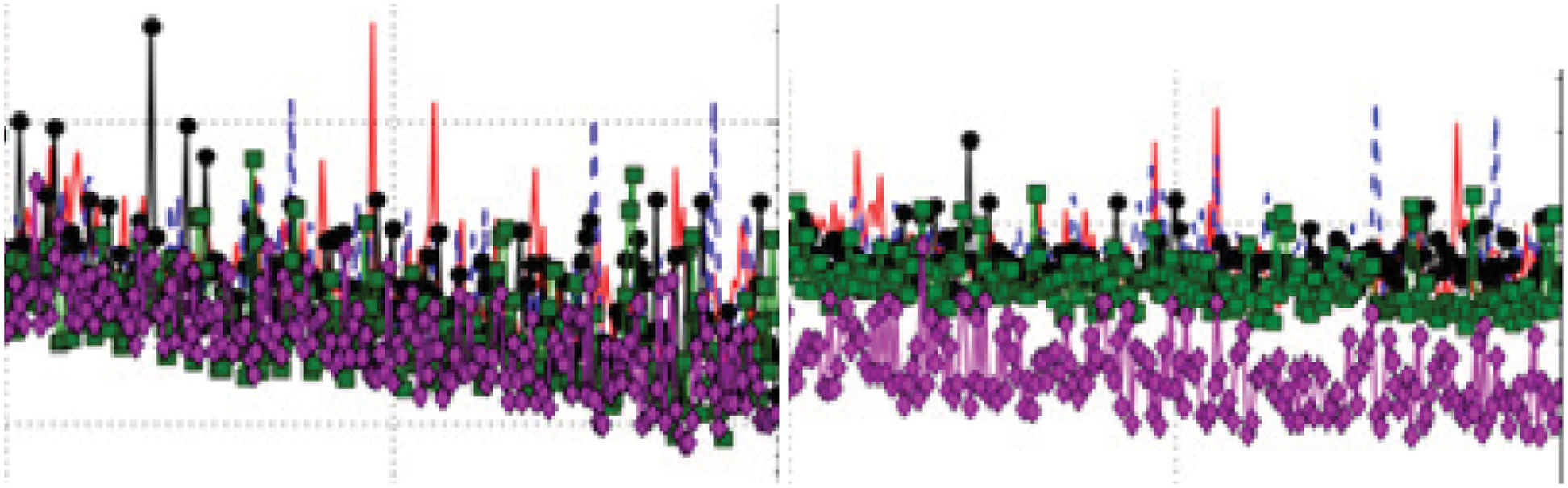
Figure 109: Optimal RNN-LSTM architecture (Section 11.3.3). Training error (a) and testing error (b), close-up views of Figure 108 from epoch 3000 to epoch 5000: Config 5 (purple line with dots) was optimal, with smaller errors than those of Config 2 (blue dashed line). See Figure 107 for config details [25]. (Figure reproduced with permission of the authors.)
11.3.4 Dual-porosity dual-permeability governing equations
The governing equations for media with dual-porosity dual-permeability in this section are only applied to macroscale (field-size) simulations, i.e., not for simulations with the microscale RVE (Figure 106, Figure 110) and with the mesoscale RVE (Figure 112, Figure 113).
For field-size simulations, assuming stationary conditions, small deformations, incompressibility, no mass exchange among solid and fluid constituents, the problem is governed by the balance of linear momentum and the balance of fluid mass in micropores and macropores, respectively. The displacement field of the solid
where
The balance of linear momemtum equation is written as
where
where
with
In the 1-D case, Darcy’s law is written as
where
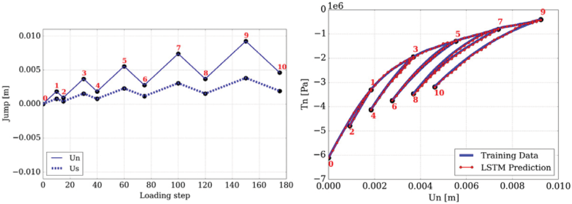
Figure 110: Mesoscale RNN with LSTM units. Traction-separation law (Sections 11.3.3, 11.3.5). Left: Sequence of imposed displacement jumps on microscale RVE (Figure 106), normal (solid line) and tangential (dotted line, with
Remark 11.5. Dimension of
Another way to verify is to identify the right-hand side of Eq. (406) with the usual inertia force per unit volume:
The empirical relation Eq. (408) adopted in [25] implies that the dimension of
i.e., mass density, whereas permeability has the dimension of area (
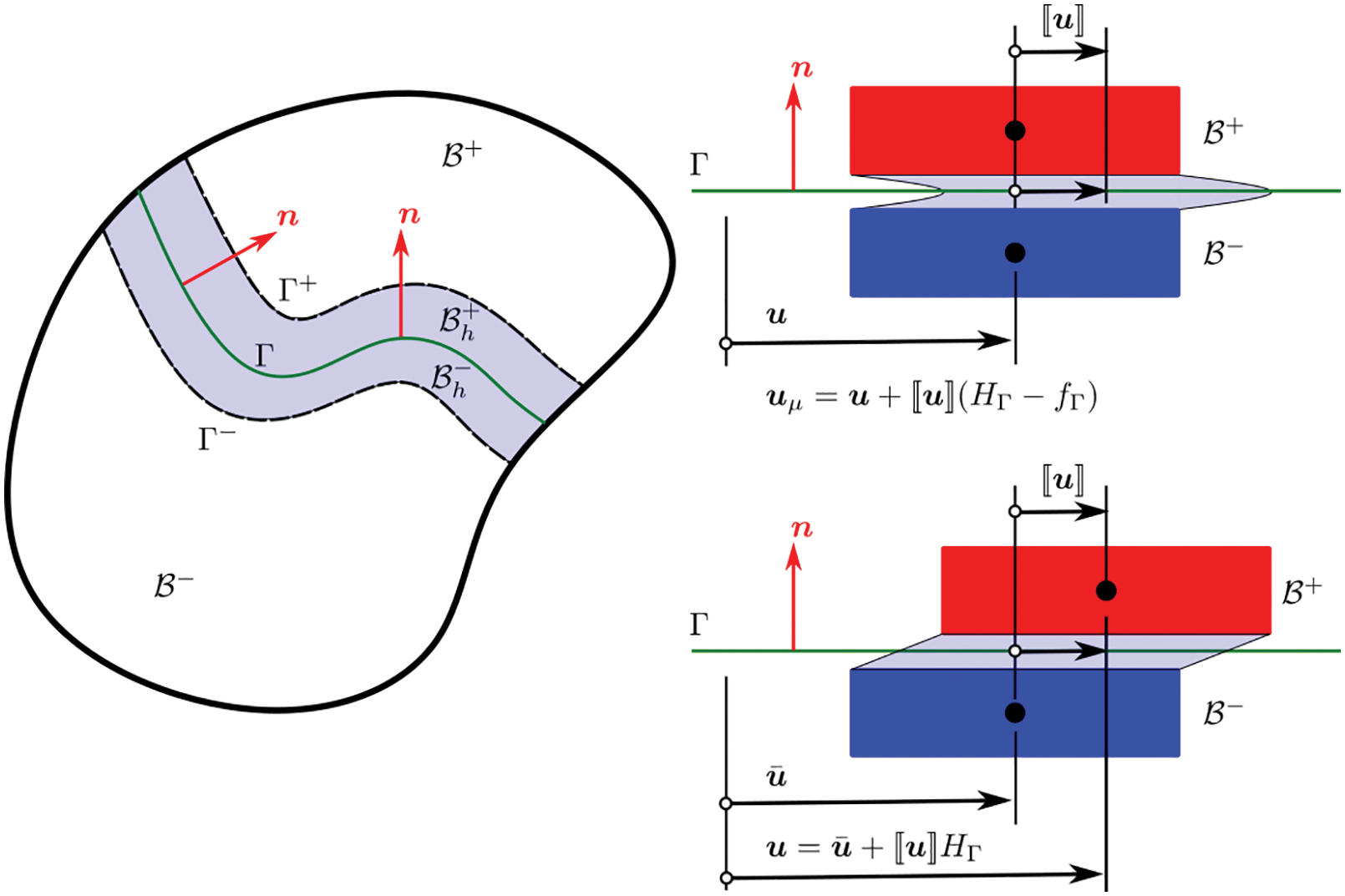
Figure 111: Continuum with embedded strong discontinuity (Section 11.3.5). Domain
The (local) porosity
The absolute macropore flux
There is a conservation of fluid transfer between the macropores and the micropores across any closed surface
Generalizing Eq. (409) to 3-D, Darcy’s law in tensor form governs the fluid mass fluxes
where
From Eq. (415), assuming that
where
agreeing with [25].
Remark 11.6. It can be verified from Eq. (417) that the dimension of
agreeing with Eq. (411). In view of Remark 11.5, for all three governing Eq. (406), Eqs. (418)-(419) to be dimensionally consistent,
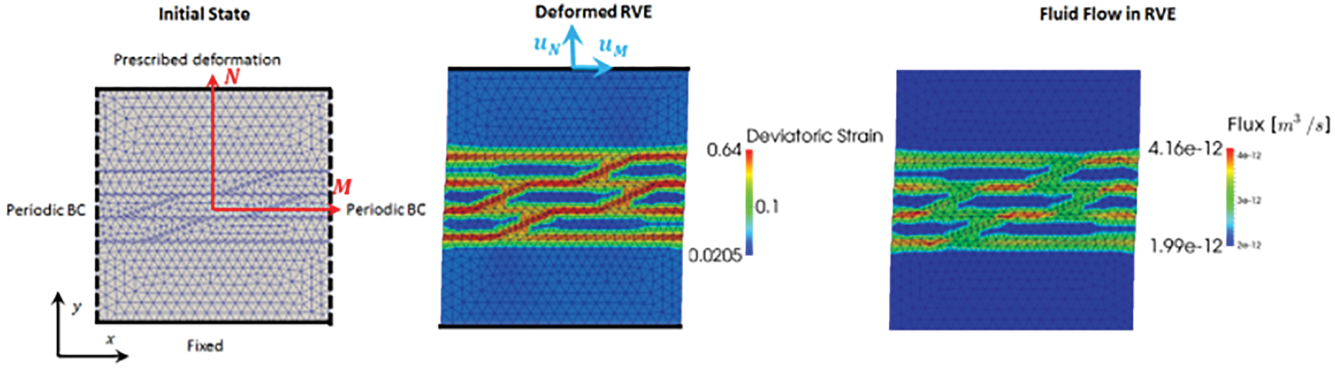
Figure 112: Mesoscale RVE (Sections 11.3.3, 11.3.5). A 2-D domain of size
Remark 11.7. For field-size simulations, the above equations do not include the changing size of the pores, which were assumed to be of constant size, and thus constant porosity, in [25]. As a result, the collapse of the pores that leads to nonlinearity in the stress-strain relation observed in experiments (Figure 13) is not modelled in [25], where the nonlinearity essentially came from the embedded strong discontinuities (displacement jumps) and the associated traction-separation law obtained from DEM simulations using the micro RVE in Figure 106 to train the meso RNN with LSTM; see Section 11.3.5. See also Remark 11.10. ■
11.3.5 Embedded strong discontinuities, traction-separation law
Strong discontinuities are embedded at both the mesocale and the macroscale. Once a fault is formed through cracks in rocks, it could become inactive (no further slip) due to surrounding stresses, friction between the two surfaces of a fault, cohesive bond, and low fluid pore pressure. A fault can be reactivated (onset of renewed fault slip) due to changing stress state, loosened fault cohesion, high fluid pore-pressure. Conventional models for fault reactivation are based on effective stresses and Coulomb law [298]:
where
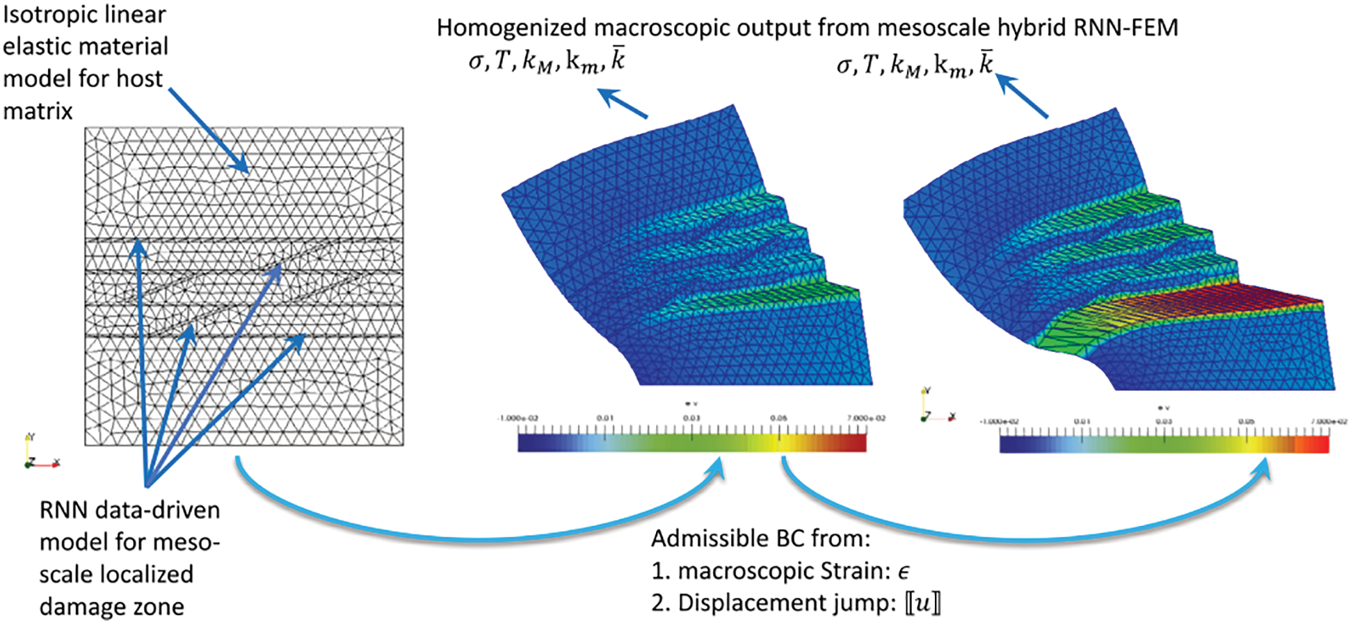
Figure 113: Mesoscale RVE (Section 11.3.3). Strains and displacement jumps [25]. (Figure reproduced with permission of the authors.)
But criterion Eq. (421) involves only stresses, with no displacement, and thus cannot be used to quantify the amount of fault slip. To allow for quantitative modeling of fault slip, or displacement jump, in a displacement-driven FEM environment, the so-called “cohesive traction-separation laws,” expressing traction (stress) vector on fault surface as a function of fault slip, similar to those used in modeling cohesive zone in nonlinear fracture mechanics [301], is needed. But these classical “cohesive traction-separation law” are not appropriate for handling loading-unloading cycles.
To model a continuum with displacement jumps, i.e., embedded strong discontinuities, the traction-separation law was represented in [25] as
where
It was assumed in [25] that cracks were pre-existing and did not propagate (see the mesoscale RVE in Figure 113), then set out to use the microscale RVE in Figure 106 to generate training data and test data for the mesocale RNN with LSTM units, called the “Mesoscale data-driven constitutive model”, to represent the traction-separation law for porous media. Their results are shown in Figure 110.
Remark 11.8. The microscale RVE in Figure 106 did not represent any real-world porous rock sample such the Majella limestone with macroporosity
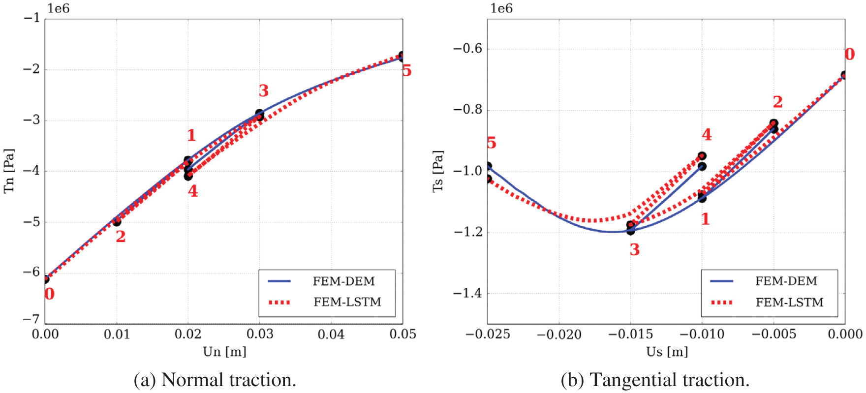
Figure 114: Mesoscale RVE (Section 11.3.5). Validation of coupled FEM and RNN with LSTM units (FEM-LSTM, red dotted line) against coupled FEM and DEM (FEM-DEM, blue line) to analyze the mesoscale RVE in Figure 113 under a sequence of imposed displacement jumps at the top (represented by numbers). (a) Normal traction (Tn) vs normal displacement (Un). (b) Tangential traction (Ts) vs tangential displacement (Us) [25]. (Figure reproduced with permission of the authors.)
Remark 11.9. Even though in Figure 14 (row 2) in Section 2.3.2, the mesoscale RVE was indicated to be of centimeter size, but the mesoscale RVE in Figure 113 was of size
To analyze the mesoscale RVE in Figure 113 (Figure 104, center) and the macroscale (field-size) model (Figure 104, right) by finite elements, both with embedded strong discontinuities (Figure 111), the authors of [25] adopted a formulation that looked similar to [297] to represent strong discontinuities, which could result from fractures or shear bands, by the local displacement field
which differs from the global smooth displacement field
Eq. (423)3 was the starting point in [297], but without using the definition of
with
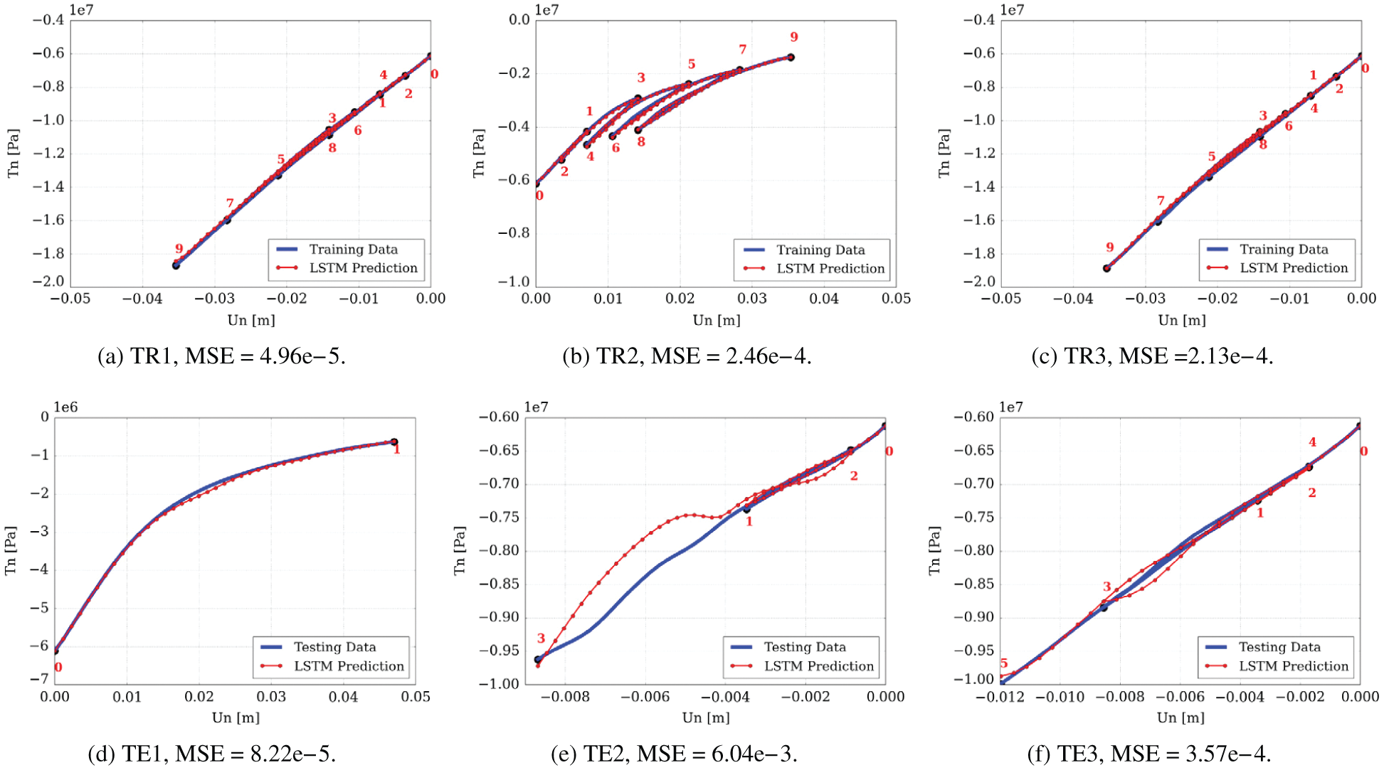
Figure 115: Macroscale RNN with LSTM units (Section 11.3.5). Normal traction (Tn) vs imposed displacement jumps (Un) on mesoscale RVE (Figure 112, Figure 113). Blue: Training data (TR1-TR3) and test data (TE1-TE3) from the mesoscale FEM-LSTM model, where numbers indicate the sequence of loading-unloading steps similar to those in Figure 110 for the mesoscale RNN with LSTM units. Red: Corresponding predictions of the trained macroscale RNN with LSTM units. The mean squared error (MSE) was used as loss function [25]. (Figure reproduced with permission of the authors.)
Later in [297], an equation that looked similar to Eq. (423)1, but in rate form, was introduced:276
where
which, when removing the overhead dot, is similar to, but different from, the small strain expression in [25], written as
where the first term was
Typically, in this type of formulation [297], once the traction-separation law
At this point, it is no longer necessary to review further this continuum formulation for displacement jumps to return to the training of the macroscale RNN with LSTM units, which the authors of [25] called the “Macroscale data-driven constitutive model” (Figure 14, row 3, right), using the data generated from the simulations using the mesoscale RVE (Figure 113) and the mesoscale RNN with LSTM units, called the “Mesoscale data-driven constitutive model” (Figure 14, row 2, right), obtained earlier.
The mesoscale RNN with LSTM units (“mesoscale data-driven constitutive model”) was first validated using the mesoscale RVE with embedded discontinuities (Figure 113), discretized into finite elements, and subjected to imposed displacements at the top. This combined FEM and RNN with LSTM units on the mesoscale RVE is denoted FEM-LSTM, with results compared well with those obtained from the coupled FEM and DEM (denoted as FEM-DEM), as shown in Figure 114.
Once validated, the FEM-LSTM model for the mesocale RVE was used to generate data to train the macroscale RNN with LSTM units (called “Macroscale data-driven constitutive model”) by imposing displacement jumps at the top of the mesoscale RVE (Figure 112), very much like what was done with the microscale RVE (Figure 106, Figure 110), just at a larger scale.
The accuracy of the macroscale RNN with LSTM units (“Macroscale data-driven constitutive model”) is illustrated in Figure 115, where the normal tractions under displacement loading were compared to results obtained with the mesoscale RVE (Figure 112, Figure 113), which was used for generating the training data. Once established, the macroscale RNN with LSTM units is used in field-size macroscale simulations. Since there is no further interesting insights into the use of deep learning, we stop of review of [25] here.
Remark 11.10. No non-linear stress-strain relation. In the end, the authors of [25] only used Figure 12 to motivate the double porosity (in Majella limestone) in their macroscale modeling and simulations, which did not include the characteristic non-linear stress-strain relation found experimentally in Majella limestone as shown in Figure 13. All nonlinear responses considered in [25] came from the nonlinear traction-separation law obtained from DEM simulations in which the particles themselves were elastic, even though the Hertz contact force-displacement relation was nonlinear [303] [304] [302]. See Remark 11.7. ■
Remark 11.11. Physics-Informed Neural Networks (PINNs) applied to solid mechanics. The PINN method discussed in Section 9.5 has been applied to problems in solid mechanics [305]: Linear elasticity (square plate, plane strain, trigonometric body force, with exact solution), nonlinear elasto-plasticity (perforated plate with circular hole, under plane-strain condition and von-Mises elastoplasticity, subjected to uniform extension, showing localized shear band). Less accuracy was encountered for solutions that presented discontinuiies (localized high gradients) in the materials properties or at the boundary conditions; see Remark 7.7 and Remark 9.5. ■
12 Application 3: Fluids, turbulence, reduced-order models
The general ideas behind the work in [26] were presented in Section 2.3.3 further above. In this section, we discuss some details of the formulation, starting with a brief primer on Proper Orthogonal Decomposition (POD) for unfamiliar readers.
12.1 Proper orthogonal decomposition (POD)
The presentation of the continuous formulation of POD in this section follows [306]. Consider the separation of variables of a time-dependent function
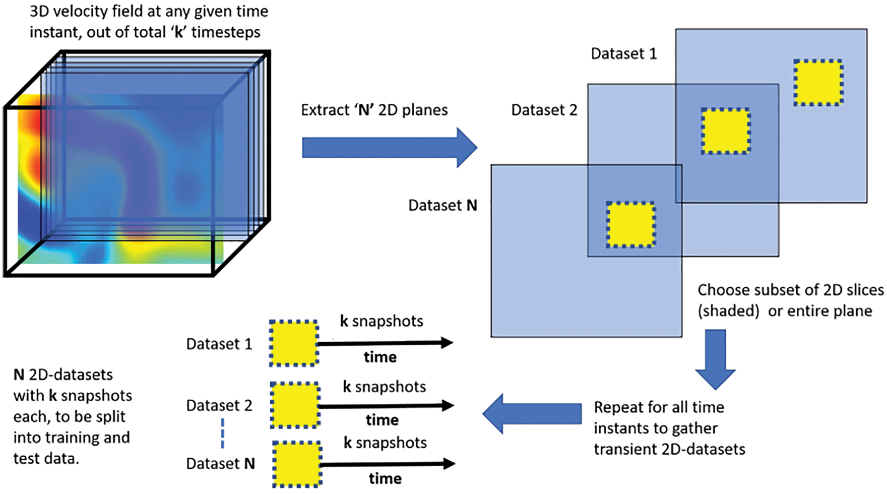
Figure 116: 2-D datasets for training neural networks (Sections 2.3.3, 12.1). Extract 2-D datasets from 3-D turbulent flow field evolving in time. From the 3-D flow field, extract
where
i.e., if
where
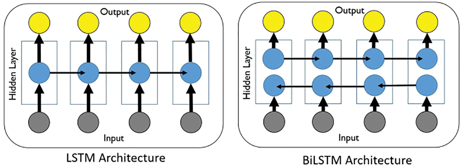
Figure 117: LSTM unit and BiLSTM unit (Sections 2.3.2, 2.3.3, 7.2, 12.2). Each blue dot is an original LSTM unit (in folded form Figure 81 in Section 7.2, without peepholes as shown in Figure 15), thus a single hidden layer. The above LSTM architecture (left) in unfolded form corresponds to Figure 82, with the inputs at state
which is equivalent to maximizing the amplitude
so that λ is the component (or projection) of the term in square brackets in Eq. (434) along the direction
which is a continuous eigenvalue problem with the eigenpair being
The coherent structure
As a result of the discrete nature of Eq. (436) and Eq. (437), the eigenvalue problem in Eq. (435) is discretized into
where the matrix
which is called a proper orthogonal decomposition of
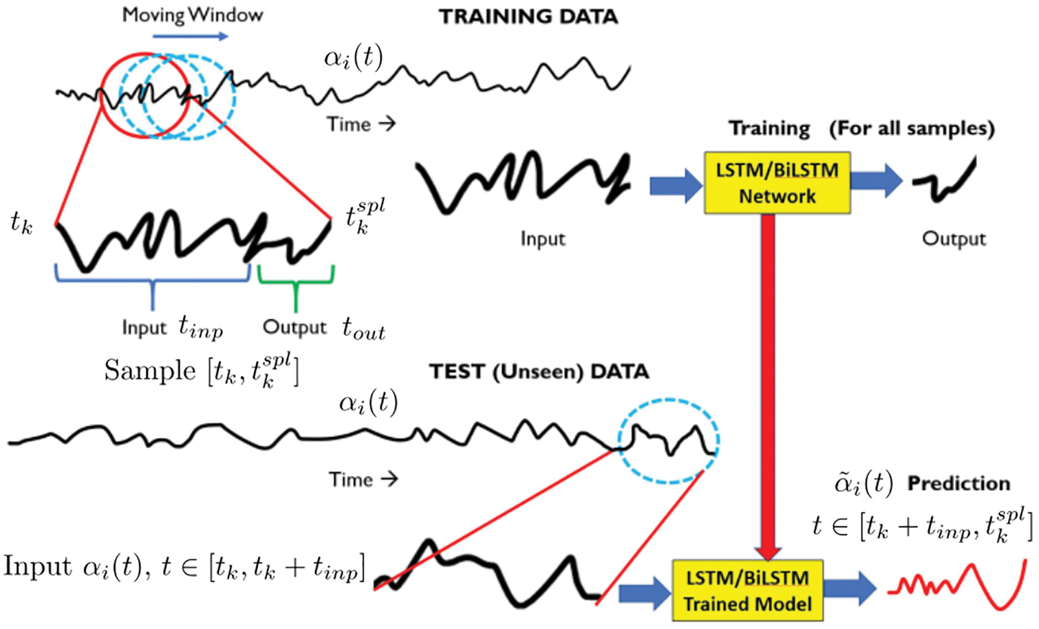
Figure 118: LSTM/BiLSTM training strategy (Sections 12.2.1, 12.2.2). From the 1-D time series
Usually, a subset of
One way is to select the POD modes corresponding to the highest eigenvalues (or energies) in Eq. (435); see Step (2) in Section 12.2.2.
Remark 12.1. Reduced-order POD. Data for two physical problems were available from numerical simulations: (1) the Force Isotropic Turbulence (ISO) dataset, and (2) the Magnetohydrodynamic Turbulence (MHD) dataset [105]. For each physical problem, the authors of [26] employed
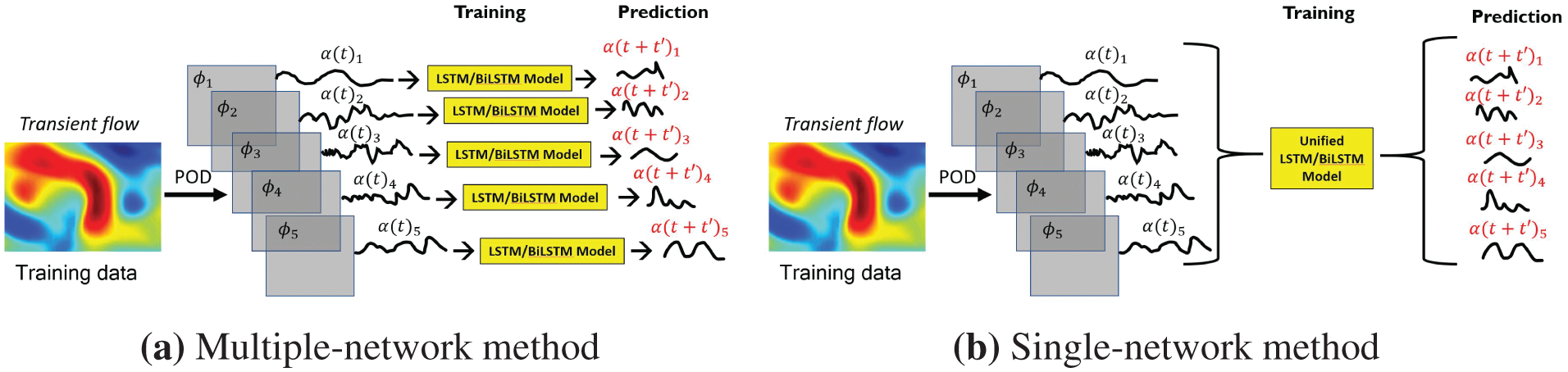
Figure 119: Two methods of developing LSTM-ROM (Section 2.3.3, 12.2.2). For each physical problem (ISO or MHD): (a) Each dominant POD mode has a network to predict
Remark 12.2. Another method of finding the POD modes without forming the symmetric matrix
12.2 POD with LSTM-Reduced-Order-Model
Typically, once the dominant POD modes of a physical problem (ISO or MHD) were identified, a reduced-order model (ROM) can be obtained by projecting the governing partial differential equations (PDEs) onto the basis of the dominant POD modes using, e.g., Galerkin projection (GP). Using this method, the authors of [306] employed full-order simulations of the governing electro-magnetic PDE with certain input excitation to generate POD modes, which were then used to project similar PDE with different parameters and solved for the coefficients
12.2.1 Goal for using neural network
Instead of using GP on the dominant POD modes of a physical problem to solve for the coefficients
To achive this goal, LSTM/BiLSTM networks (Figure 117) were trained using thousands of paired short input / output signals obtained by segmenting the time-dependent signal
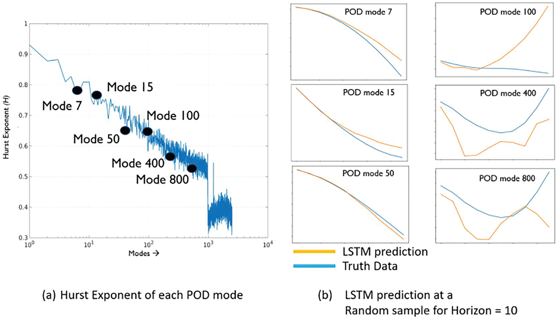
Figure 120: Hurst exponent vs POD-mode rank for Isotropic Turbulence (ISO) (Sections 12.3). POD modes with larger eigenvalues (Eq. (438)) are higher ranked, and have lower rank number, e.g., POD mode rank 7 has larger eigenvalue, and thus more dominant, than POD mode rank 50. The Hurst exponent, even though fluctuating, trends downward with the POD mode rank, but not monotonically, i.e., for two POD modes sufficiently far apart (e.g., mode 7 and mode 50), a POD mode with lower rank generally has a lower Hurst exponent. The first 800 POD modes for the ISO problem have the Hurst exponents higher than 0.5, and are thus persistent [26]. (Adapted with permission of the author.)
12.2.2 Data generation, training and testing procedure
The following procedure was adopted in [26] to develop their LSTM-ROM for two physical problems, ISO and MHD; see Remark 12.1. For each of the two physical problems (ISO and MHD), the following steps were used:
(1) From the 3-D computational domain of a physical problem (ISO or MHD), select
(2) For each of the training datasets and test datasets, extract from
(3) The time series of the coefficient
(4) Use the input/output pairs generated from the training datasets in Step (3) to train LSTM/BiLSTM-ROM networks. Two methods were considered in [26]:
(a) Multiple-network method: Use a separate RNN for each of the
(b) Single-network method: Use the same RNN to predict the coefficients
The single-network method better captures the inter-modal interactions that describe the energy transfer from larger to smaller scales. Vortices that spread over multiple dominant POD modes also support the single-network method, which does not artificially constrain flow features to separate POD modes.
(5) Validation: Input/output pairs similar to those for training in Step (3) were generated from the test dataset for validation.279 With a short time series of the coefficient
(6) At time
12.3 Memory effects of POD coefficients on LSTM models
The results and deep-learning concepts used in [26] were presented in the motivational Section 2.3.3 above, Figure 20. In this section, we discuss some details of the formulation.
Remark 12.3. Even though the value of
The “U-velocity field for all results” was mentioned in [26], but without a definition of “U-velocity”, which was possibly the
The BiLSTM networks in the numerical examples were not as accurate as the LSTM networks for both physical problems (ISO and MHD), despite having more computations; see Figure 117 above and Figure 20 in Section 2.3.3. The authors of [26] conjectured that a reason could be due to the randomness nature of turbulent flows, as opposed to the high long-term correlation found in natural human languages, for which BiLSTM was designed to address.
Since LSTM architecture was designed specifically for sequential data with memory, it was sought in [26] to quantify whether there was “memory” (or persistence) in the time series of the coefficients
where
A Hurst coefficient of
The effects of prediction horizon and persistence on the prediction accuracy of LSTM network were studied in [26]. Horizon is the number of steps after the input sample that a LSTM model would predict the values of
To this end, they selected one dataset (training or testing), and followed the multiple-network method in Step (4) of Section 12.2.2 to develop a different LSTM network model for each POD mode with “non-negligible eigenvalue”. For both the ISO (Figure 120) and MHD problems, the 800 highest ranked POD modes were used.
A baseline horizon of 10 steps were used, for which the prediction errors were
Another expected result was that for the same POD mode rank lower than 50, the error increased dramatically with the prediction horizon. For example, for POD rank 7, the errors were
A final note is whether the above trained LSTM-ROM networks could produce accurate prediction for flow dynamics with different parameters such as Reynolds number, mass density, viscosity, geometry, initial conditions, etc., particularly that both the ISO and MHD datasets were created for a single Reynolds number, which was not mentioned in [26], who mentioned that their method (and POD in general) would work for a “narrow range of Reynolds numbers” for which the flow dynamics is qualitatively similar, and for “simplified flow fields and geometries”.
Remark 12.4. Use of POD-ROM for different systems. The authors of [306] studied The flexibility of POD reduced-order models to solve nonlinear electromagnetic problems by varying the excitation form (e.g., square wave instead of sine wave) and by using the undamped (without the first-order time derivative term) snapshots in the simulation of the damped case (with the first-order time derivative term). They demonstrated via numerical examples involving nonlinear power-magnetic-component simulations that the reduced-order models by POD are quite flexible and robust. See also Remark 12.2. ■
Remark 12.5. pyMOR - Model Order Reduction with Python. Finally, we mention the software pyMOR,281 which is “a software library for building model order reduction applications with the Python programming language. Implemented algorithms include reduced basis methods for parametric linear and non-linear problems, as well as system-theoretic methods such as balanced truncation or IRKA (Iterative Rational Krylov Algorithm). All algorithms in pyMOR are formulated in terms of abstract interfaces for seamless integration with external PDE (Partial Differential Equation) solver packages. Moreover, pure Python implementations of FEM (Finite Element Method) and FVM (Finite Volume Method) discretizations using the NumPy/SciPy scientific computing stack are provided for getting started quickly.” It is noted that pyMOR includes POD and “Model order reduction with artificial neural networks”, among many other methods; see the documentation of pyMOR. Clearly, this software tool would be applicable to many physical problems, e.g., solids, structures, fluids, electromagnetics, coupled electro-thermal simulation, etc. ■
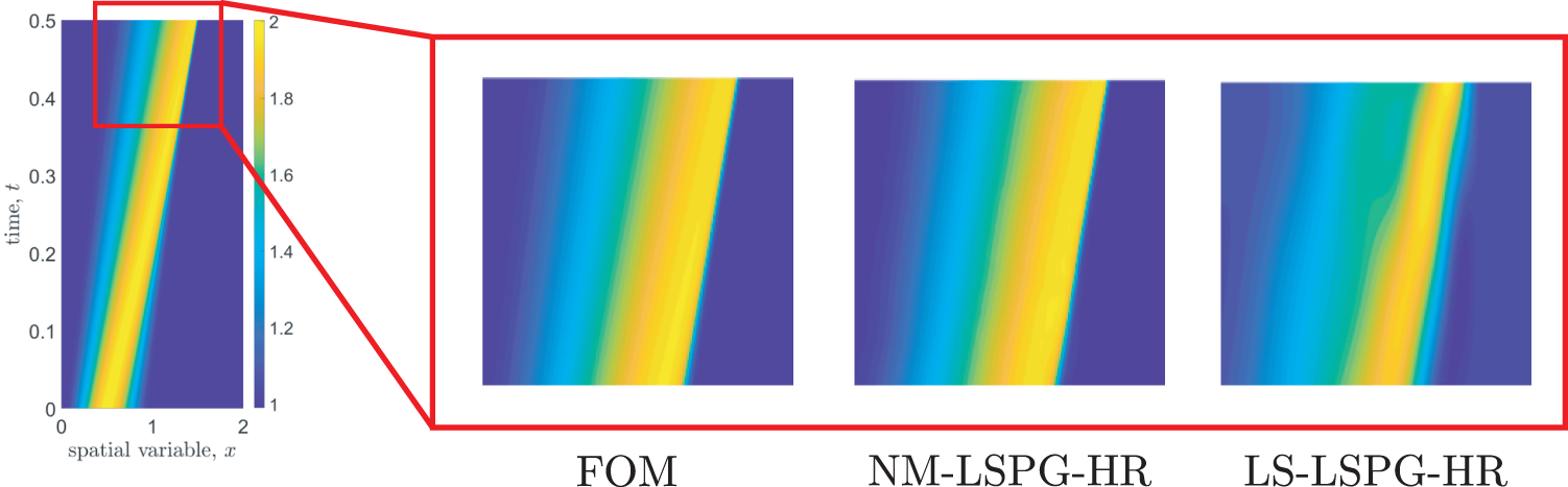
Figure 121: Space-time solution of inviscid 1D-Burgers’ equation (Section 12.4.1). The solution shows a characteristic steep spatial gradient, which shifts and further steepens in the course of time. The FOM solution (left) and the solution of the proposed hyper-reduced ROM (center), in which the solution subspace is represented by a nonlinear manifold in the form of a feedforward neural network (Section 4) (NM-LSPG-HR), show an excellent agreement, whereas the spatial gradient is significantly blurred in the solution obtained with a hyper-reduced ROM based on a linear subspace (LS-LSPG-HR) (right). The FOM is a obtained upon a finite-difference approximation in the spatial domain with
12.4 Reduced order models and hyper-reduction
Reduction of computational expense also is the main aim of nonlinear manifold reduced-order models (NM-ROMs), which have recently been proposed in [47],282 where the approach belongs to the class of projection-based methods. Projection-based methods rely on the idea that solutions to physical simulations lie in a subspace of small dimensionality as compared to the dimensionality of high-fidelity models, which we obtain upon discretization (e.g., by finite elements) of the governing equations. In classical projection-based methods, such “intrinsic solution subspaces” are spanned by a set of appropriate basis vectors that capture the essential features of the full-order model (FOM), i.e., the subspace is assumed to be linear. We refer to [307] for a survey on projection-based linear subspace methods for parametric systems.283
12.4.1 Motivating example: 1D Burger’s equation
The effectiveness of linear subspace methods is directly related to the dimensionality of the basis to represent solutions with sufficient accuracy. Advection-dominated problems and problems with solutions that exhibit large (“sharp”) gradients, however, are characterized by a large Kolmogorov
Burger’s equation serves as a common prototype problem in numerical methods for nonlinear partial differential equations (PDEs) and MOR, in particular. The inviscid Burgers’ equation in one spatial dimension is given by
Burgers’ equation is a first-order hyperbolic equation which admits the formation of shock waves, i.e., regions with steep gradients in field variables, which propagate in the domain of interest. Its left-hand side corresponds to material time-derivatives in Eulerian descriptions of continuum mechanics. In the balance of linear momentum, for instance, the field
The above initial conditions are governed by a scalar parameter
Figure 121 shows a zoomed view of solutions to the above problem obtained with the FOM (left), the proposed nonlinear manifold-based ROM (NM-LSPG-HR, center) and a conventional ROM, in which the full-order solution is represented by a linear subspace. The initial solution is characterized by a “bump” in the left half of the domain, which is centered at
The ROM based on a linear subspace of the full-order solution (LS-LSPG-HR) fails to accurately reproduce the steep spatial gradient that develops over time, see Figure 121, right Instead, the bump is substantially blurred in the linear subspace-based ROM as compared to the FOM’s solution (left). The maximum error over all time steps
where
The solution manifold can be represented by means of a shallow, sparsely connected feed-forward neural network [47] (see Statics, feedforward networks, Sections 4, 4.6). The network is trained in an unsupervised manner using the concept of autoencoders (see Autoencoder, Section 12.4.3).
12.4.2 Nonlinear manifold-based (hyper-)reduction
The NM-ROM approach proposed in [47] addressed nonlinear dynamical systems, whose evolution was governed by a set of nonlinear ODEs, which had been obtained by a semi-discretization of the spatial domain, e.g., by means of finite elements:
In the above relation,
The fundamental idea of any projection-based ROM is to approximate the original solution space of the FOM by a comparatively low-dimensional space
Using the nonlinear function
where
where the Jacobian
Note that linear subspace methods are included in the above relations as the special case where
As opposed to the nonlinear manifold Eq. (449), the tangent space of the (linear) solution manifold is constant, i.e.,
The authors of [47] defined a residual function
As
Requiring the derivative of the (squared) residual to vanish, we obtain the following set of equations,287
which can be rearranged for the rate of the reduced vector of generalized coordinates as:
The above system of ODEs, in which
An alternative approach was also presented in [47] for the construction of ROMs, in which time-discretization was performed prior to the projection onto the low-dimensional solution subspace. For this purpose a uniform time-discretization with a step size
The above integration rule implies that span of rate
For the backward Euler scheme Eq. (455), a residual function was defined in [47] as the difference
Just as in the time-continuous domain, the system of equations
To solve the least-squares problem, the Gauss-Newton method with starting point
Unlike the time-continuous case, the Gauss-Newton method results in a projection involving not only the Jacobian
Within the NS-ROM approach, it was proposed in [47] to construct
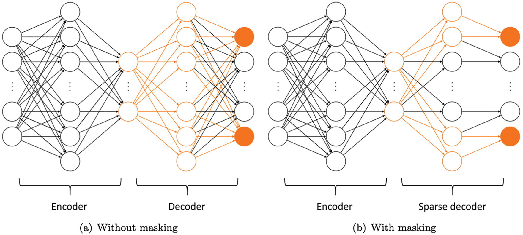
Figure 122: Dense vs. shallow decoder networks (Section 12.4.3). Contributing neurons (orange “nodes”) and connections (orange “edges”) lie in the “active” paths arriving at the selected outputs (solid orange “nodes”) from the decoder’s inputs. In dense networks as the one in (a), each neuron in a layer is connected to all other neurons in both the preceeding layer (if it exists) and in the succeeding layer (if it exists). Fully-connected networks are characterized by dense weight matrices, see Section 4.4. In sparse networks as the decoder in (b), several connections among successive layers are dropped, resulting in sparsely populated weight matrices. (Figure reproduced with permission of the authors.)
As the above relation reveals, autoencoders are typically composed from two parts, i.e.,
The input data, which was formed by the snapshots of solutions
is such that each component of the normalized input ranges from
The decoder reconstructs the high-dimensional solution
where the operator ⊘ denotes the element-wise division. The composition of encoder and decoder give the autoencoder, i.e.,
which is trained in an unsupervised way to (approximately) reproduce states
Both the encoder and the decoder are feed-forward neural networks with a single hidden layer. As activation function, it was proposed in [47] to use the sigmoid function (see Figure 30 and Section 13.3.1) or the swish function (see Figure 139). It remains unspecified, however, which of the two were used in the numerical examples in [47]. Though the representational capacity of neural networks increases with depth, which is what ‘deep learning’ is all about, the authors of [47] deliberately used shallow networks to minimize the (computational) complexity of computing the decoder’s Jacobian
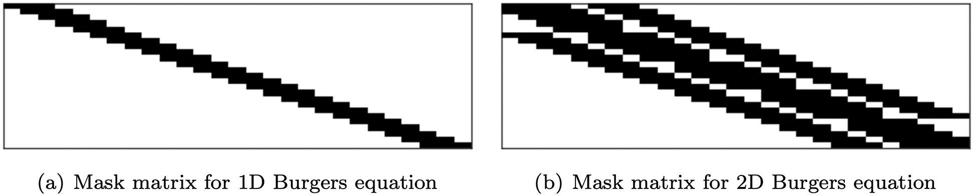
Figure 123: Sparsity masks (Section 12.4.3) used to realize sparse decoders in one- and two-dimensional problems. The structure of the respective binary-valued mask matrices
Using our notation for feedforward networks and activation functions introduced in Section 4.4, the encoder network has the following structure:
where
The structure of the sparsity mask
Irrespective of how small the dimensionality of the ROM’s solution subspace
In [47], a variant of GNAT relying on solution snapshots for the approximation of the nonlinear residual term
In DEIM methods, the residual
The matrix
The matrix
Substituting the above result in Eq. (467), the FOM’s residual can be interpolated using an oblique projection matrix
The above representation in terms of the projection matrix
Several methods have been proposed to efficiently construct a suitable set of sampling indices
The reduced-order vector
The key idea of the greedy algorithm is to select additional indices to minimize the error of the gappy reconstruction. Therefore, the component of the reconstructed mode that differs most (in terms of magnitude) from the original mode defines the
A pseudocode representation of the greedy approach for selecting sampling indices is given in Algorithm 8. To start the algorithm, the first sampling index is chosen according to the largest (in terms of magnitude) component of the first POD-mode, i.e.,
The authors of [47] substituted the residual vector
From the above minimization problem, the ROM’s ODEs were determined in [47] by taking the derivative with respect to the reduced vector of generalized velocities

where the definition of the residual vector
which, using the notion of the pseudo-inverse, is resolved for
Remark 12.6. Equivalent minimization problems. Note the subtle difference between the minimization problems that govern the ROMs with and without hyper-reduction, see Eqs. (452) and (474), respectively: For the case without hyper-reduction, see Eq. (452), the minimum is sought for the approximate full-dimensional residual
Repeating the steps of the derivation in Eq. (475) then gives
i.e., using the identity
Remark 12.7. Further reduction of the system operator? At first glance, the operator in the ROM’s governing equations in Eq. (477) appears to be further reducible:
Note that the product
We first consider linear subspace methods, for which the Jacobian
Note that, in linear subspace methods, the operator
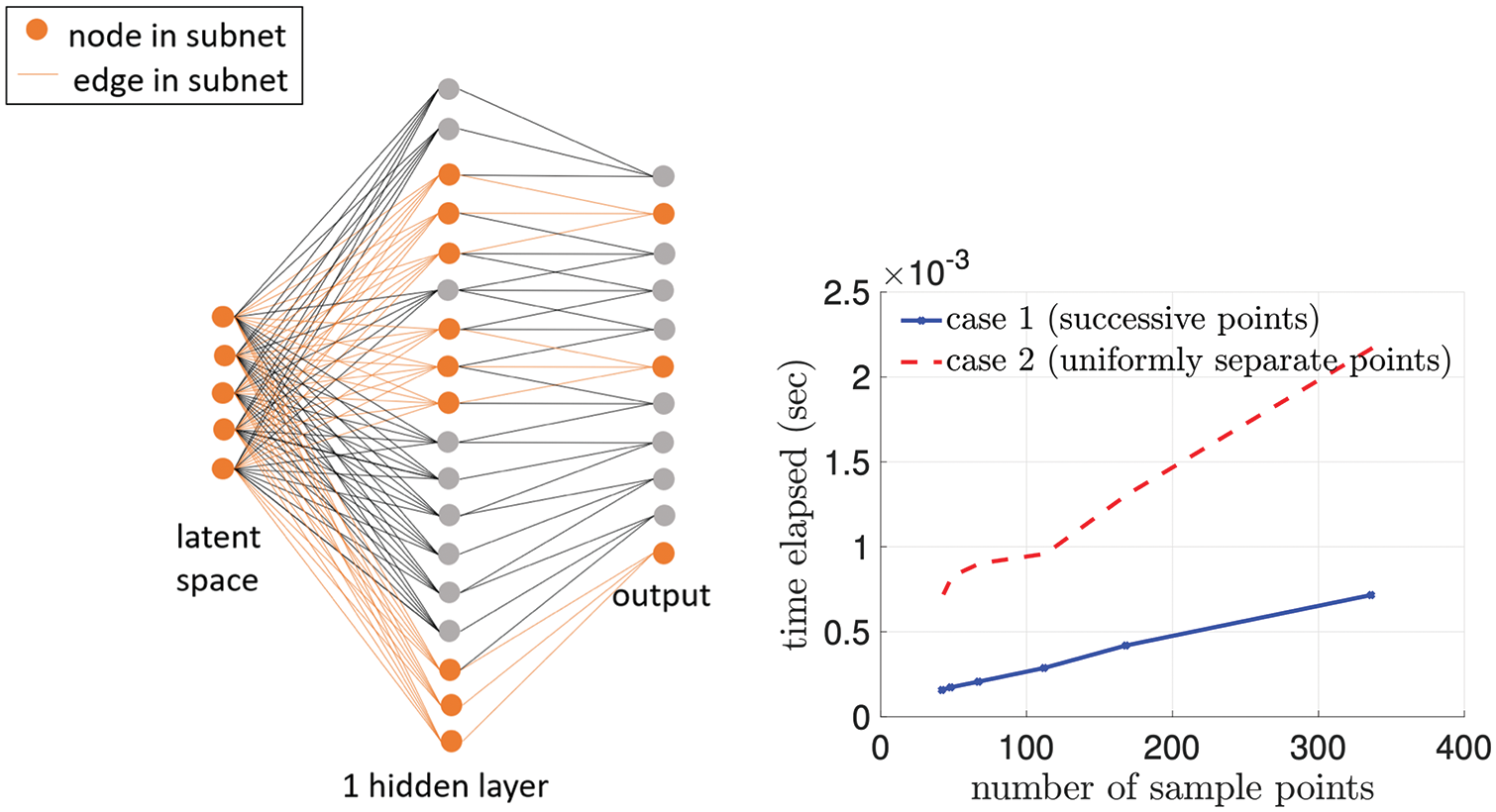
Figure 124: Subnet construction (Section 12.4.4). To reduce computational cost, a subnet representing the set of active paths, which comprise all neurons and connections needed for the evaluation of selected outputs (highlighted in orange), i.e., the reduced residual
Instead, only those rows of
By keeping track of which components of full-order solution
To explain this discrepancy, assume the full-order model to be obtained upon a finite-element discretization. Given some particular nodal point, all finite elements sharing the node contribute to the corresponding components of the nonlinear function
For nonlinear manifold methods, we cannot expect much improvement in computational efficiency by the hyper-reduction. As a matter of fact, the ‘nonlinearity’ becomes twofold if the reduced subspace is a nonlinear manifold: We do not only have to compute selected components of the nonlinear term
For Petrov-Galerkin-type variants of ROMs, hyper-reduction works in exactly the same way as with their Galerkin counterparts. The residual in the minimization problem in Eq. (458) is approximated by a gappy reconstruction, i.e.,
From a computational point of view, the same implications apply to Petrov-Galerkin ROMs as for Galerkin-type ROMs, which is why we focus on the latter in our review.
In the approach of [47], the nonlinear manifold
The computational cost of evaluating the decoder and its Jacobian scales with the number of parameters of the neural network. Both shallowness and sparsity of the decoder network already account for computational efficiency in regard of the number of parameters.
Additionally, the authors of [47] traced “active paths” when evaluating selected components of the decoder and its Jacobian of the hyper-reduced model. The set of active paths comprises all those connections and neurons of the decoder network which are involved in evaluations of its outputs. Figure 124 (left) highlights the active paths for the computations of the components of the reduced residual
Given all active paths, a subnet of the decoder network is constructed to only evaluate those components of the full-order state which are required to compute the hyper-reduced residual. The computational costs to compute the residual and its Jacobian depends on the size of the subnet. As both input and output dimension are given, size translates into width of the (single) hidden layer. The size of the hidden layer, in turn, depends on the distribution of the sampling indices
For the sparsity patterns assumed, successive output components show the largest overlap in terms of the number of neurons in the hidden layer involved in the evaluation, whereas the overlap is minimal in case of equally spaced outputs.
The cases of successive and equally distributed sampling indices constitute extremal cases, for which the computational time for the evaluation of both the residual and its Jacobian of the 2D-example (Section 12.4.5) are illustrated as a function of the dimensionality of the reduced residual (“number of sampling points”) in Figure 124 (right).
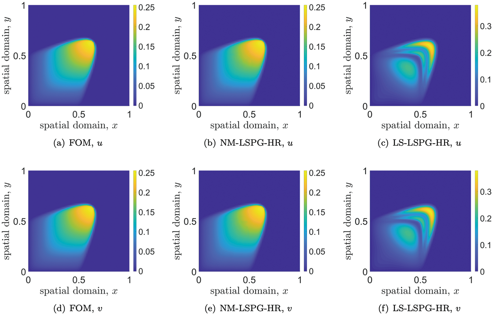
Figure 125: 2-D Burger’s equation. Solution snapshots of full and reduced-order models (Section 12.4.5). From left to right, the components
12.4.5 Numerical example: 2D Burger’s equation
As a second example, consider now Burgers’ equation in two (spatial) dimensions [47], instead of in one dimension as in Section 12.4.1. Additionally, viscous behavior, which manifests as the Laplace term on the right-hand side of the following equation, was included as opposed to the one-dimensional problem in Eq. (442):
The problem was solved on a square (unit) domain
An inhomogeneous flow profile under 45 ° was prescribed as initial conditions (
where
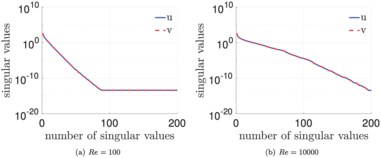
Figure 126: 2-D Burger’s equation. Reynolds number vs. singular values (Section 12.4.5). Performing SVD on FOM solution snapshots, which were partitioned into
The semi-discrete FOM was a finite-difference approximation in the spatial dimension on a uniform
where
For time integration, the backward Euler scheme with a constant step size
Figure 126 shows the influence of the Reynolds number on the singular values obtained from solution snapshots of the FOM. For
Both autoencoders (for
To evaluate the accuracy of the NM-ROMs proposed in [47], the Burgers’ equation was solved for the target parameter
The authors of [47] also studied the impact how the size of the parameter set
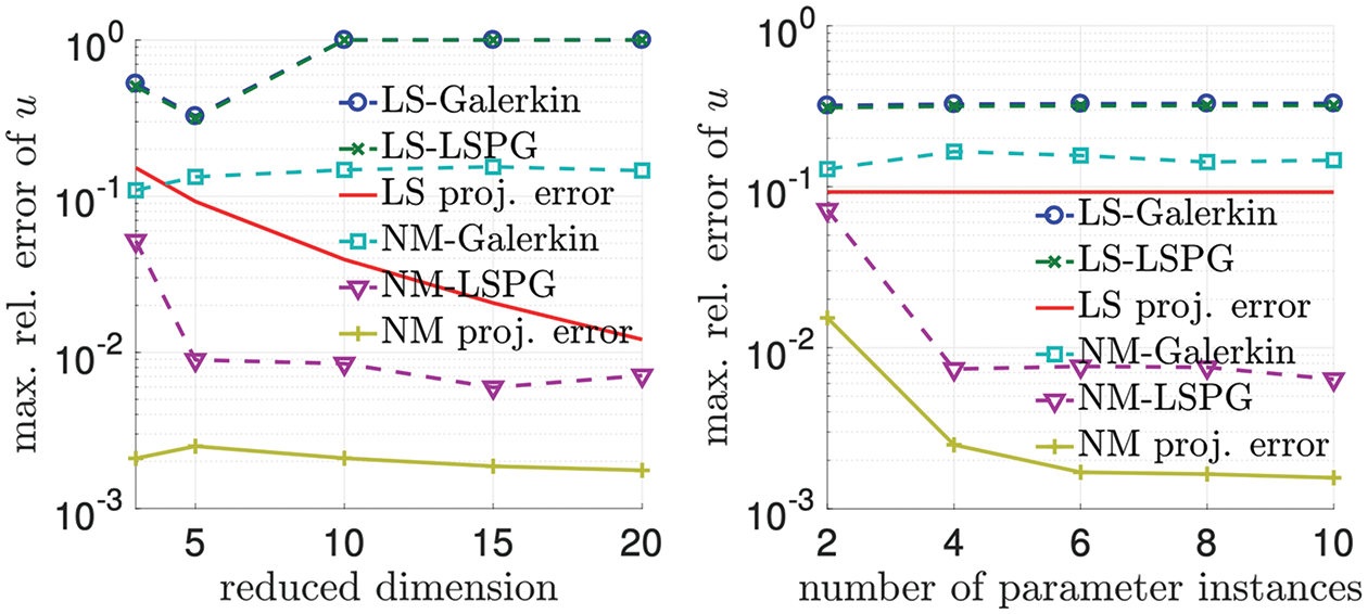
Figure 127: 2D-Burgers’ equation: relative errors of nonlinear manifold and linear subspace ROMs (Section 12.4.5). (Figure reproduced with permission of the authors.)
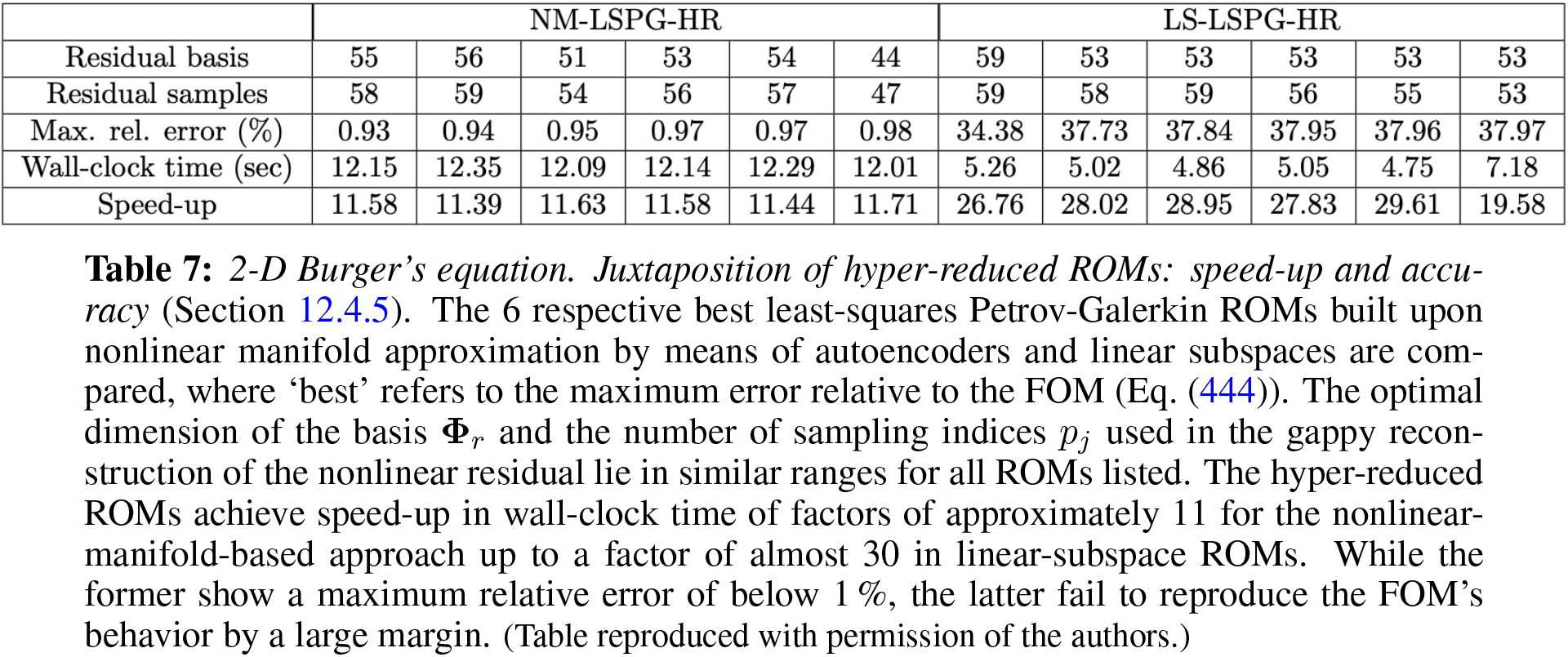
the reduced dimension was set to
Hyper-reduction turned out to be crucial with respect to computational efficiency. For a reduced dimension of
Figure 128: Machine-learning accelerated CFD (Section 12.4.5). Speed-up factor, compared to direct integration, was much higher than those obtained from nonlinear model-order reduction in Table 7 [317]. Permission of NAS.
Figure 129: Machine-learning accelerated CFD (Section 12.4.5). Good accuracy and good generalization, devoiding of non-physical solutions [317]. Permission of NAS.
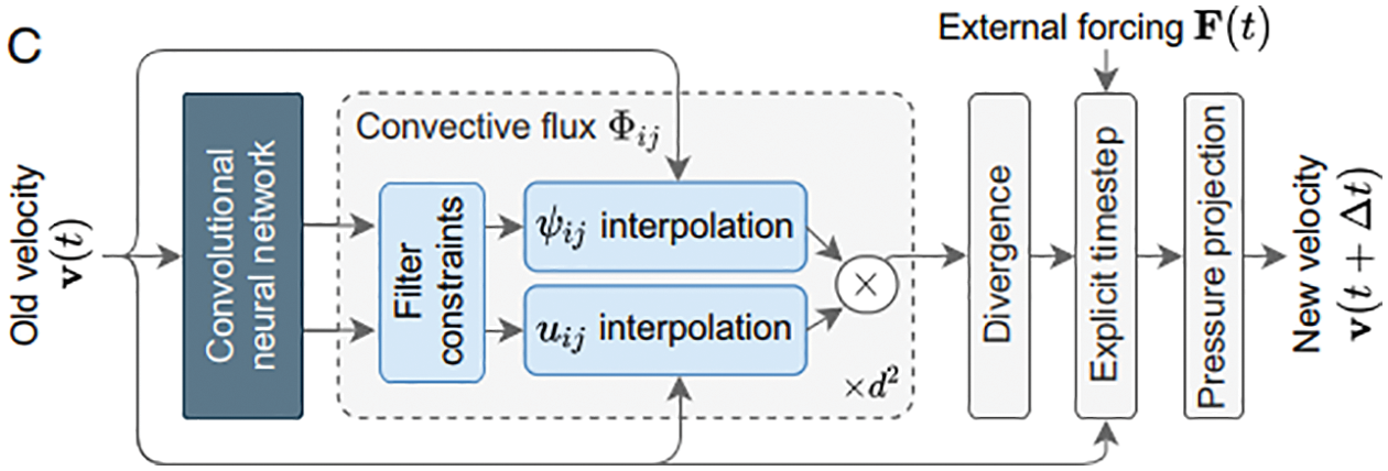
Figure 130: Machine-learning accelerated CFD (Section 12.4.5). The neural network generates interpolation coefficients based on local-flow properties, while ensuring at least first-order accuracy relative to the grid spacing [317]. Permission of NAS.
Remark 12.8. Machine-learning accelerated CFD. A hybrid method between traditional direct integration of the Navier-Stokes equation and machine learning (ML) interpolation was presented in [317] (Figure 130), where a speed-up factor close to 90, many times higher than those in Table 7, was obtained, Figure 128, while generalizing well (Figure 129). Grounded on the traditional direct integration, such hybrid method would avoid non-physical solutions of pure machine-learning methods, such as the physics-inspired machine learning (Section 9.5, Remark 9.4), maintain higher accuracy as obtained with direct integration, and at the same time benefit from an acceleration from the learned interpolation. ■
Remark 12.9. In concluding this section, we mention the 2023 review paper [318], brought to our attention by a reviewer, on “A state-of-the-art review on machine learning-based multiscale modeling, simulation, homogenization and design of materials.” This review paper would nicely complement our present review paper. ■
13.1 Early inspiration from biological neurons
In the early days, many papers on artificial neural networks, particularly for applications in engineering, started to motivate readers with a figure of a biological neuron as in Figure 131 (see, e.g., [23], Figure 1a), before displaying an artificial neuron (e.g, [23], Figure 1b). When artificial neural networks took a foothold in the research community, there was no need to motivate with a biological neuron, e.g., [38] [20], which began directly with an artificial neuron.
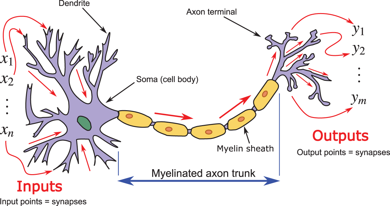
Figure 131: Biological Neuron and signal flow (Sections 4.4.4, 13.1, 13.2.2) along myelinated axon, with inputs at the synapses (input points) in the dendrites and with outputs at the axon terminals (output points,which are also the synapses for the next neuron). Each input current
13.2 Spatial / temporal combination of inputs, weights, biases
Both [21] and [78] referred to Rosenblatt (1958) [119], who first proposed using a linear combination of inputs with weights, and with biases (thresholds). The authors of [78], p. 14, only mentioned the “linear model” defined—using the notation convention in Eq. (16)—as
without the bias. On the other hand, it was written in [21] that “Rosenblatt proposed a simple rule to compute the output. He introduced weights, real numbers expressing the importance of the respective inputs to the output” and “some threshold value,” and attributed the following equation to Rosenblatt
where the threshold is simply the negative of the bias
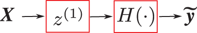
Figure 132: The perceptron network (Sections 4.5, 13.2)—introduced by Rosenblatt (1958) [119], (1962) [120]—has a linear combination with weights and bias as expressed in
Moreover, adding to the confusion for first-time learners, another error and misleading statement about the “Rosenblatt perceptron” in connection with Eq. (488) and Eq. (489)—which represent a single neuron—is in [78], p. 13, where it was stated that the “Rosenblatt perceptron” involved only a “single neuron”:
“The first wave started with cybernetics in the 1940s-1960s, with the development of theories of biological learning (McCulloch and Pitts, 1943; Hebb, 1949) and implementations of the first models, such as the perceptron (Rosenblatt, 1958), enabling the training of a single neuron.” [78], p. 13.
The error of considering the Rosenblatt perceptron as having a “single neuron” is also reported in Figure 42, which is Figure 1.11 in [78], p. 23. But the Rosenblatt perceptron as described in the cited reference Rosenblatt (1958) [119] and in Rosenblatt (1960) [319] was a network, called a “nerve net”:
“Any perceptron, or nerve net, consists of a network of “cells,” or signal generating units, and connections between them.”
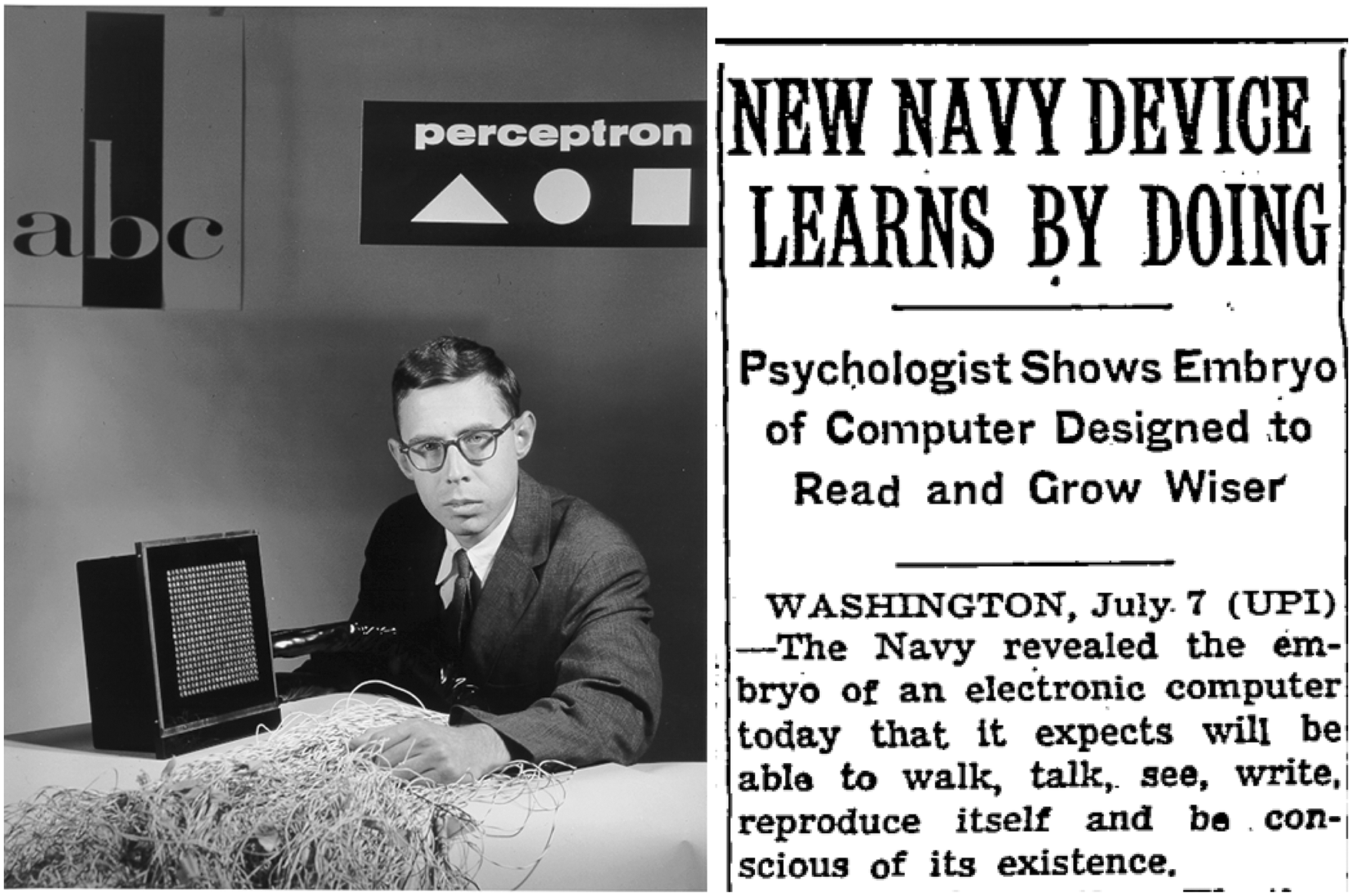
Figure 133: Rosenblatt and the Mark I computer (Sections 4.6.1, 13.2) based on the perceptron, described in the New York Times article titled “New Navy device learns by doing” on 1958 July 8 (Internet archive), as a “computer designed to read and grow wiser”, and would be able to “walk, talk, see, write, reproduce itself and be conscious of its existence. The first perceptron will have about 1,000 electronic “association cells” [A-units] receiving electrical impulses from an eye-like scanning device with 400 photo cells”. See also the Youtube video “Perceptron Research from the 50’s & 60’s, clip”. Sometimes, it is incorrectly thought that Rosenblatt’s network had only one neuron (A-unit); see Figure 42, Section 4.6.1.
Such a “nerve net” would surely not just contain a “single neuron”. Indeed, the report by Rosenblatt (1957) [1] that appeared a year earlier mentioned a network (with one layer) containing as many a thousand neurons, called “association cells” (or A-units):294
“Thus with 1000 A-units connected to each R-unit [response unit or output], and a system in which 1% of the A-units respond to stimuli of a given size (i.e.,
The perceptron with one thousand A-units mentioned in [1] was also reported in the New York Times article “New Navy device learns by doing” on 1958 July 8 (Internet archive); see Figure 133. Even if the report by Rosenblatt (1957) [1] were not immediately accessible, it was stated in no uncertain terms that the perceptron was a machine with many neurons:
“The organization of a typical photo-perceptron (a perceptron responding To optical patterns as stimuli) is shown In Figure1. ... [Rule] 1. Stimuli impinge on a retina of Sensory units (S-points), which are Assumed to respond on an all-or-nothing basis295. [Rule] 2. Impulses are transmitted to a set Of association cells (A-units) [neurons]... If the algebraic sum of excitatory and Inhibitory impulse intensities296 is equal To or greater than the threshold297 (θ) of The A-unit, then the A-unit fires, again On an all-or-nothing basis.” [119]
Figure 1 in [119] described a network (“nerve net”) with many A-units (neurons). Does anyone still read the classics anymore?
Rosenblatt’s (1962) book [2], p. 33, provided the following neuroscientific explanation for using a linear combination (weight sum / voting) of the inputs in both time and space:
“The arrival of a single (excitatory) impulse gives rise to a partial depolarization of the post-synaptic298 membrane surface, which spreads over an appreciable area, and decays exponentially with time. This is called a local excitatory state (l.e.s.). The l.e.s. due to successive impulses is (approximately) additive. Several impulses arriving in sufficiently close succession may thus combine to touch off an impulse in the receiving neuron if the local excitatory state at the base of the axon achieves the threshold level. This phenomenon is called temporal summation. Similarly, impulses which arrive at different points on the cell body or on the dendrites may combine by spatial summation to trigger an impulse if the l.e.s. induced at the base of the axon is strong enough.”
The spatial summation of the input synaptic currents is also consistent with Kirchhoff’s current law of summing the electrical currents at a junction in an electrical network.299 We first look at linear combination in the static case, followed by the dynamic case with Volterra series.
13.2.1 Static, comparing modern to classic literature
“A classic is something that everybody wants to have read and nobody wants to read.”
Mark Twain
Readers not interested in reading the classics can skip this section. Here, we will not review the perceptron algorithm,300 but focus our attention on the historical details not found in many modern references, and connect Eq. (488) and Eq. (489) to the original paper by Rosenblatt (1958) [119]. But the problem is that such task is not directly obvious for readers of modern literature, such as [78] for the following reasons:
• Rosenblatt’s work in [119] was based on neuroscience, which is confusing to those without this background;
• Unfamiliar notations and concepts for readers coming from deep-learning literature, such as [21], [78];
• The word “weight” was not used at all in [119], and thus cannot be used to indirectly search for hints of equations similar to Eq. (488) or Eq. (489);
• The word “threshold” was used several times, such as in the sentence “If the algebraic sum of excitatory and inhibitory impulse intensities is equal to or greater than the threshold (θ)”301 of the A-unit, then the A-unit fires, again on an all-or-nothing basis”. The threshold θ is used in Eq. (2) of [119]:
where
As will be shown below, it was misleading to refer to [119] for equations such as Eq. (488) and Eq. (489), even though [119] contained the seed ideas leading to these equations upon refinement as presented in [120], which was in turn based on the book by Rosenblatt (1962) [2].
Instead of a direct reading of [119], we suggest reading key publications in reverse chronological orders. We also use the original notations to help readers to identify quickly the relevant equations in the classic literature.
The authors of [121] introduced a general class of machines, each known under different names, but decided to call all these machines as “perceptrons” in honor of the pioneering work of Rosenblatt. General perceptrons were defined in [121], p. 10, as follows. Let
Let
A general perceptron was defined as a more complex predicate, denoted by ψ, which was a weighted voting or linear combination of the simple predicates in
with
The next paper to read is [120], which was based on the book by Rosenblatt (1962) [2], and from where the following equation305 can be identified as being similar to Eq. (493) and Eq. (489), again in its original notation as
where
To discriminate between two classes, the input
If the algebraic sum
Eq. (495) in [120] would correspond to Eq. (490) in [119], with the connection strengths
That Eq. (495) was not numbered in [120] indicates that it played a minor role in this paper. The reason is clear, since the author of [120] stated307 that “the connections
Moreover, the very first sentence in [120] was “The perceptron is a self-organizing and adaptive system proposed by Rosenblatt”, and the book by [2] was immediately cited as Ref. 1, whereas only much later in the fourth page of [120] did the author write “With the Perceptron, Rosenblatt offered for the first time a model...”, and cited Rosenblatt’s 1958 report first as Ref. 34, followed by the paper [119] as Ref. 35.
In a major work on AI dedicated to Rosenblatt after his death in a boat accident, the authors of [121], p.xi, in the Prologue of their book, referred to Rosenblatt’s (1962) book [2] and not Rosenblatt’s (1958) paper [119]:
“The 1960s: Connectionists and Symbolists
Interest in connectionist networks revived dramatically in 1962 with the publication of Frank Rosenblatt’s book Principles of Neurodynamics in which he defined the machines he named perceptrons and proved many theories about them.”
In fact, Rosenblatt’s (1958) paper [119] was never referred to in [121], except for a brief mention of the influence of “Rosenblatt’s [1958]” work on p. 19, without the full bibliographic details. The authors of [121] wrote:
“However, it is not our goal here to evaluate these theories [to model brain functioning], but only to sketch a picture of the intellectual stage that was set for the perceptron concept. In this setting, Rosenblatt’s [1958] schemes quickly took root, and soon there were perhaps as many as a hundred groups, large and small, experimenting with the model either as a ‘learnÂing machine’ or in the guise of ‘adaptive’ or ‘self-organizing’ networks or ‘automatic control’ systems.”
So why was [119] often referred to for Eq. (488) or Eq. (489), instead of [120] or [2],308 which would be much better references for these equations? One reason could be that citing [120] would not do justice to [119], which contained the germ of the idea, even though not as refined as four years later in [120] and [2]. Another reason could be the herd effect by following other authors who referred to [119], without actually reading the paper, or without comparing this paper to [120] or [2]. A best approach would be to refer to both [119] and [120], as papers like these would be more accessible than books like [2].
Remark 13.1. The hype on the Rosenblatt perceptron Mark I computer described in the 1958 New York Times article shown in Figure 133, together with the criticism of the Rosenblatt perceptron in [121] for failing to represent the XOR function, led to an early great disappointment on the possibilities of AI when overreached expectations for such device did not pan out, and contributed to the first AI winter that lasted until the 1980s, with a resurgence in interest due to the development of backpropagation and application in psychology as reported in [22]. But some sixty years since the Mark I computer, AI still cannot even think like human babies yet: “Understanding babies and young children may be one key to ensuring that the current “AI spring” continues—despite some chilly autumnal winds in the air” [321]. ■
13.2.2 Dynamic, time dependence, Volterra series
For time-dependent input
where
with the continuous linear combination (weighted sum) appearing in the second term. The convolution integral in Eq. (497) is the basis for convolutional networks for highly effective and efficient image recognition, inspired by mammalian visual system. A review of convolutional networks outside the scope here, despite them being the “greatest success story of biologically inspired artificial intelligence” [78], p. 353.
For biological neuron models, both The input
Eq. (497) is the continuous temporal summation, counterpart of the discrete spatial summation in Eq. (26), with the constant term
where
i.e., the continuous weighted sum
Remark 13.2. The discrete counterpart of the linear part of the Volterra series in Eq. (497) can be found in the exponential-smoothing time series in Eq. (212), with the kernel
In firing-rate models of the brain (see Figure 27), the function
For a neuron with
with
Using the synaptic kernel Eq. (498) in Eq. (500) for the total somatic input
Remark 13.3. The second term in Eq. (501), with time-independent input
As a result, the subscript ∞ is often used to denote as the steady state solution, such as
For constant total somatic input
where
At this stage, there are two possible firing-rate models. The first firing-rate model consists of (1) Eq. (501), the ODE for the total somatic input firing rate
Remark 13.4. The steady-state output
where
The second firing-rate model consists of using Eq. (501) for the total somatic input firing rate
where the activation function
Eq. (507) is a recurring theme that has been frequently used in papers in neuroscience and artificial neural networks. Below are a few relevant papers for this review, particularly the continuous recurrent neural networks (RNNs)—such as Eq. (510), Eq. (512), and Eqs. (515)-(516)—which are the counterparts of the discrete RNNs in Section 7.1.
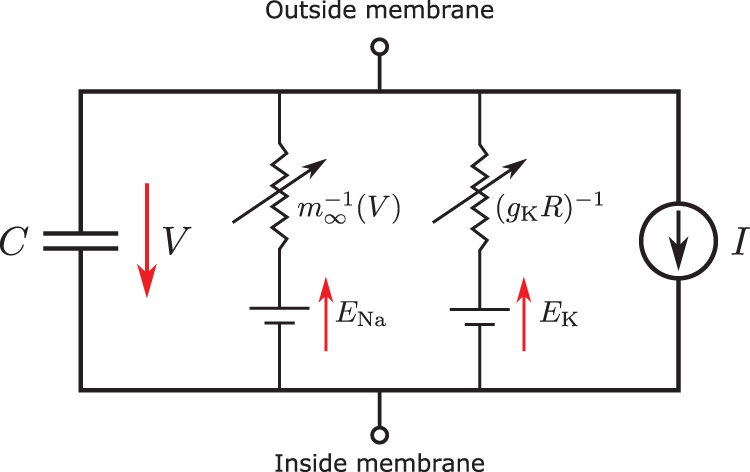
Figure 134: Model of neocortical neurons in [118] as a simplification of the model in [322] (Section 13.2.2): A capacitor
The model for neocortical neurons in [118], a simplification of the model by [322], was employed in [116] as starting point to develop a formulation that produced SubFigure(b) in Figure 28 consists of two coupled ODE’s317
where
To create a continuous recurrent neural network described by ODEs in Eq. (510), the input
The network is called symmetric if the weight matrix is symmetric, i.e.,
The difference between Eq. (510) and Eq. (507) is that Eq. (507) is based on the expression for
A time-dependent time delay
where the diagonal matrix
For discrete RNNs, the delay is a constant integer set to one, i.e.,
as expressed in Eq. (275) in Section 7.1.
Both Eq. (510) and Eq. (512) can be rewritten in the following form:
A densely distributed pre-synaptic input points [see Eq. (500) and Figure 131 of a biological neurons] can be approximated by a continuous distribution in space, represented by
where
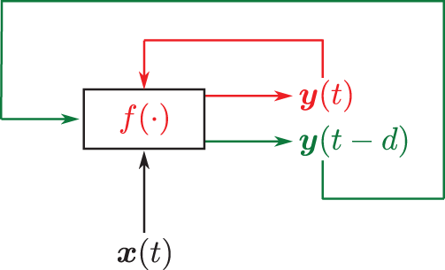
Figure 135: Continuous recurrent neural network with time-dependent delay
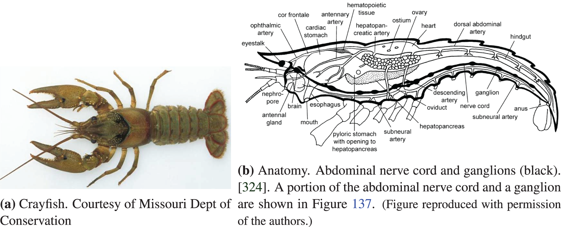
Figure 136: Crayfish (Section 13.3.2), freshwater crustaceans. Anatomy.
The use of the logistic sigmoid function (Figure 30) in neuroscience dates back since the seminal work of Nobel Laureates Hodgkin & Huxley (1952) [322] in the form of an electrical circuit (Figure 134), and since the work reported in [35] in a form closer to today’s network; see also [325] and [37].
The authors of [78], p. 219, remarked: “Despite the early popularity of rectification (see next Section 13.3.2), it was largely replaced by sigmoids in the 1980s, perhaps because sigmoids perform better when neural networks are very small.”
The rectified linear function has, however, made a come back and was a key component responsible for the success of deep learning, and helped inspired a variant that in 2015 surpassed human-level performance in image classification, as “it expedites convergence of the training procedure [16] and leads to better solutions [21, 8, 20, 34] than conventional sigmoid-like units” [61]. See Section 5.3.3 on Parametric Rectified Linear Unit.
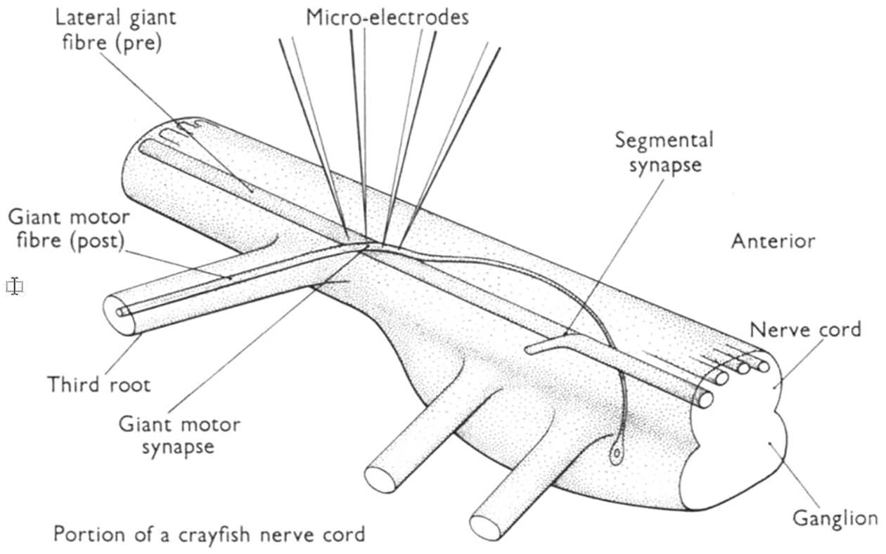
Figure 137: Crayfish giant motor synapse (Section 13.3.2). The (pre-synaptic) lateral giant fiber was connected to the (post-synaptic) giant motor fiber through a synapse where the two fibers cross each other at the location annotated by “Giant motor synapse” in the figure. This synapse was right underneath the giant motor fiber, at the crossing and contact point, and thus could not be seen. The two left electrodes (including the second electrode from left) were inserted in the lateral giant fiber, with the two right electrodes in the giant motor fiber. Currents were injected into the two electrodes indicated by solid red arrows, and electrical outputs recorded from the two electrodes indicated by dashed blue arrows [326]. (Figure reproduced with permission of the publisher Wiley.)
13.3.2 Rectified linear unit (ReLU)
Yoshua Bengio, the senior author of [78] and a Turing Award recipient, recounted the rise in popularity of ReLU in deep learning networks in an interview in [79]:
“The big question was how we could train deeper networks... Then a few years later, we discovered that we didn’t need these approaches [Restricted Boltzmann Machines, autoencoders] to train deep networks, we could just change the nonlinearity. One of my students was working with neuroscientists, and we thought that we should try rectified linear units (ReLUs)—we called them rectifiers in those days—because they were more biologically plausible, and this is an example of actually taking inspiration from the brain. We had previously used a sigmoid function to train neural nets, but it turned out that by using ReLUs we could suddenly train very deep nets much more easily. That was another big change that occurred around 2010 or 2011.”
The student mentioned by Bengio was likely the first author of [113]; see also the earlier Section 4.4.2 on activation functions.
We were aware of Ref. [32] appearing in year 2000—in which a spatially-discrete, temperally-continuous recurrent neural network was used with a rectified linear function, as expressed in Eq. (510)—through Ref. [36]. On the other hand, prior its introduction in deep neural networks, rectified linear unit had been used in neuroscience since at least 1995, but [327] was a book, as cited in [113]. Research results published in papers would appear in book form several years later:
“ The current and third wave, deep learning, started around 2006 (Hinton et al., 2006; Bengio et al., 2007; Ranzato et al., 2007a) and is just now appearing in book form as of 2016. The other two waves [cybernetics and connectionism] similarly appeared in book form much later than the corresponding scientific activity occurred” [78], p. 13.
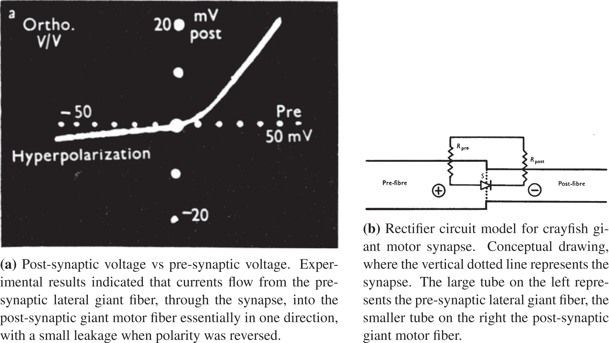
Figure 138: Crayfish Giant Motor Synapse (Section 13.3.2). The response in SubFigure (a) is similar to that of a rectifier circuit with leaky diode in Figure 25 and Figure 29 [red curve (
Another clue that the rectified linear function was a well-known, well accepted concept—similar to the relation
Indeed, more than sixty years ago, in a series of papers [58] [326] [59], Furshpan & Potter established that current flows through a crayfish neuron synapse (Figure 136 and Figure 137) in essentially one direction, thus deducing that the synapse can be modeled as a rectifier, diode in series with resistance, as shown in Figure 138.
“The design of hidden units is an extremely active area of research and does not yet have many definitive guiding theoretical principles,” [78], p. 186. Indeed, the Swish activation function in Figure 139 of the form
with
On the other hand, it would be hard to beat the efficiency of the rectified linear function in both evaluating the weighted combination of inputs
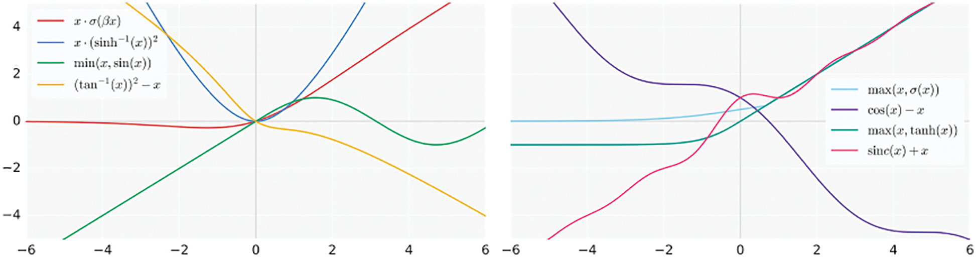
Figure 139: Swish function (Section 13.3.3)
A zoo of activation functions is provided in “Activation function”, Wikipedia, version 22:46, 24 November 2018 and the more recent version 06:30, 20 July 2022, in which several active functions had been removed, e.g., the “Square Nonlinearity (SQNL)”321 listed in the 2018 version of this zoo.
13.4 Back-propagation, automatic differentiation
“At its core, backpropagation [Section 5] is simply an efficient and exact method for calculating all the derivatives of a single target quantity (such as pattern classification error) with respect to a large set of input quantities (such as the parameters or weights in a classification rule)” [328].
In a survey on automatic differentiation in [329], it was stated that: “in simplest terms, backpropagation models learning as gradient descent in neural network weight space, looking for the minima of an objective function.”
Such statement identified back-propagation with an optimization method by gradient descent. But according to the authors of [78], p. 198, “back-propagation is often misunderstood as meaning the whole learning algorithm for multilayer neural networks”, and clearly distinguish back-propagation only as a method to compute the gradient of the cost function with respect to the parameters, while another algorithm, such as stochastic gradient descent, is used to perform the learning using this gradient, where performing “learning” meant network training, i.e., find the parameters that minimize the cost function, which “typically includes a performance measure evaluated on the entire training set as well as additional regularization terms.”322
According to [329], automatic differentiation, or in short “autodiff”, is “a family of techniques similar to but more general than backpropagation for efficiently and accurately evaluating derivatives of numeric functions expressed as computer programs.”
In an interview published in 2018 [79], Hinton confirmed that backpropagation was independently invented by many people before his own 1986 paper [22]. Here we focus on information that is not found in the review of backpropagation in [12].
For example, the success reported in [22] laid not in backpropagation itself, but in its use in psychology:
“Back in the mid-1980s, when computers were very slow, I used a simple example where you would have a family tree, and I would tell you about relationships within that family tree. I would tell you things like Charlotte’s mother is Victoria, so I would say Charlotte and mother, and the correct answer is Victoria. I would also say Charlotte and father, and the correct answer is James. Once I’ve said those two things, because it’s a very regular family tree with no divorces, you could use conventional AI to infer using your knowledge of family relations that Victoria must be the spouse of James because Victoria is Charlotte’s mother and James is Charlotte’s father. The neural net could infer that too, but it didn’t do it by using rules of inference, it did it by learning a bunch of features for each person. Victoria and Charlotte would both be a bunch of separate features, and then by using interactions between those vectors of features, that would cause the output to be the features for the correct person. From the features for Charlotte and from the features for mother, it could derive the features for Victoria, and when you trained it, it would learn to do that. The most exciting thing was that for these different words, it would learn these feature vectors, and it was learning distributed representations of words.” [79]
For psychologists, “a learning algorithm that could learn representations of things was a big breakthrough,” and Hinton’s contribution in [22] was to show that “backpropagation would learn these distributed representations, and that was what was interesting to psychologists, and eventually, to AI people.” But backpropagation lost ground to other technologies in machine learning:
“In the early 1990s, ... the support vector machine did better at recognizing handwritten digits than backpropagation, and handwritten digits had been a classic example of backpropagation doing something really well. Because of that, the machine learning community really lost interest in backpropagation” [79].323
Despite such setback, psychologists still considered backpropagation as an interesting approach, and continued to work with this method:
There is “a distinction between AI and machine learning on the one hand, and psychology on the other hand. Once backpropagation became popular in 1986, a lot of psychologists got interested in it, and they didn’t really lose their interest in it, they kept believing that it was an interesting algorithm, maybe not what the brain did, but an interesting way of developing representations” [79].
The 2015 review paper [12] referred to Werbos’ 1974 PhD dissertation for a preliminary discussion of backpropagation (BP),
“Efficient BP was soon explicitly used to minimize cost functions by adapting control parameters (weights) (Dreyfus, 1973). Compare some preliminary, NN-specific discussion (Werbos, 1974, Section 5.5.1), a method for multilayer threshold NNs (Bobrowski, 1978), and a computer program for automatically deriving and implementing BP for given differentiable systems (Speelpenning, 1980).”
and explicitly attributed to Werbos early applications of backpropagation in neural networks (NN):
“To my knowledge, the first NN-specific application of efficient backpropagation was described in 1981 (Werbos, 1981, 2006). Related work was published several years later (LeCun, 1985, 1988; Parker, 1985). A paper of 1986 significantly contributed to the popularization of BP for NNs (Rumelhart, Hinton, & Williams, 1986), experimentally demonstrating the emergence of useful internal representations in hidden layers.”
See also [112] [328] [330]. The 1986 paper mentioned above was [22].
13.4.2 Automatic differentiation
The authors of [78], p. 214, wrote of backprop as a particular case of automatic differentiation (AD):
“The deep learning community has been somewhat isolated from the broader computer science community and has largely developed its own cultural attitudes concerning how to perform differentiation. More generally, the field of automatic differentiation is concerned with how to compute derivatives algorithmically. The back-propagation algorithm described here is only one approach to automatic differentiation. It is a special case of a broader class of techniques called reverse mode accumulation.”
Let’s decode what was said above. The deep learning community was isolated because it was not in the mainstream of computer science research during the last AI winter, as Hinton described in an interview published in 2018 [79]:
“This was at a time when all of us would have been a bit isolated in a fairly hostile environment—the environment for deep learning was fairly hostile until quite recently—it was very helpful to have this funding that allowed us to spend quite a lot of time with each other in small meetings, where we could really share unpublished ideas.”
If Hinton did not move from Carnegie Mellon University in the US to the University of Toronto in Canada, it would be necessary for him to change research topic to get funding, AI winter would last longer, and he may not get the Turing Award along with LeCun and Bengio [331]:
“The Turing Award, which was introduced in 1966, is often called the Nobel Prize of computing, and it includes a $1 million prize, which the three scientists will share.”
A recent review of AD is given in [329], where backprop was described as a particular case of AD, known as “reverse mode AD”; see also [12].324
13.5 Resurgence of AI and current state
The success of deep neural networks in the ImageNet competitions since 2012, particularly when they surpassed human-level performance in 2015 (See Figure 3 and Section 5.3.3 on Parametric ReLU), was preceded by their success in speech recognition, as recounted by Hinton in a 2018 interview [79]:
“For computer vision, 2012 was the inflection point. For speech, the inflection point was a few years earlier. Two different graduate students at Toronto showed in 2009 that you could make a better speech recognizer using deep learning. They went as interns to IBM and Microsoft, and a third student took their system to Google. The basic system that they had built was developed further, and over the next few years, all these companies’ labs converted to doing speech recognition using neural nets. Many of the best people in speech recognition had switched to believing in neural networks before 2012, but the big public impact was in 2012, when the vision community, almost overnight, got turned on its head and this crazy approach turned out to win.”
The mentioned 2009 breakthrough of applying deep learning to speech recognition did not receive much of the non-technical press as the 2012 breakthrough in computer vision (e.g., [75] [74]), and was thus not popularly known, except inside the deep-learning community.
Deep learning is being developed and used to guide consumers in nutrition [332]:
“Using machine learning, a subtype of artificial intelligence, the billions of data points were analyzed to see what drove the glucose response to specific foods for each individual. In that way, an algorithm was built without the biases of the scientists.
There are other efforts underway in the field as well. In some continuing nutrition studies, smartphone photos of participants’ plates of food are being processed by deep learning, another subtype of A.I., to accurately determine what they are eating. This avoids the hassle of manually logging in the data and the use of unreliable food diaries (as long as participants remember to take the picture).
But that is a single type of data. What we really need to do is pull in multiple types of data—activity, sleep, level of stress, medications, genome, microbiome and glucose—from multiple devices, like skin patches and smartwatches. With advanced algorithms, this is eminently doable. In the next few years, you could have a virtual health coach that is deep learning about your relevant health metrics and providing you with customized dietary recommendations.”
13.5.1 COVID-19 machine-learning diagnostics and prognostics
While it is not possible to review the vast number of papers on deep learning, it would be an important omission if we did not mention a most urgent issue of our times,325 the COVID-19 (COronaVIrus Disease 2019) pandemic, and how deep learning could help in the diagnostics and prognostics of Covid-19.
Some reviews of Covid-19 models and software. The following sweeping assertion was made in a 2021 MIT Technology Review article titled “Hundreds of AI tools have been built to catch covid. None of them helped” [334], based on two 2021 papers that reviewed and appraised the validity and usefulness of Covid-19 models for diagnostics (i.e., detecting Covid-19 infection) and for prognostics (i.e., forecasting the course of Covid-19 in patients) [335] and [336]:
“The clear consensus was that AI tools had made little, if any, impact in the fight against covid.”
A large collection of 37,421 titles (published and preprint reports) on Covid-19 models up to July 2020 were examined in [335], where only 169 studies describing 232 prediction models were selected based on CHARMS (CHecklist for critical Appraisal and data extraction for Systematic Reviews of prediction Modeling Studies) [337] for detailed analysis, with the risk of bias assessed using PROBAST (Pediction model Risk Of Bias ASsessment Tool) [338]. A follow-up study [336] examined 2,215 titles up to Oct 2020, using the same methodology as in [335] with the added requirement of “sufficiently documented methodologies”, to narrow down to 62 titles for review “in most details”. In the words of the lead developer of PROBAST, “unfortunately” journals outside the medical field were not included since it would be a “surprise” that “the reporting and conduct of AI health models is better outside the medical literature”.326
Figure 140: MIT COVID-19 diagnosis by cough recordings. Machine learning architecture. Audio Mel Frequency Cepstrum Coefficients (MFCC) as input. Each cough signal is split into 6 audio chunks, processed by the MFCC package, then passed through the Biomarker 1 to check on muscular degradation. The output of Biomarker 1 is input into each of the three Convolutional Neural Networks (CNNs), representing Biomarker 2 (Vocal cords), Biomarker 3 (Lungs & Respiratory Tract), Biomarker 4 (Sentiment). The outputs of these CNNs are concatenated and “pooled” together to serve as (1) input for “Competing Aggregator Models” to produce a “longitudinal saliency map”, and as (2) input for a deep and dense network with ReLU activation, followed by a “binary dense layer” with sigmoid activation to produce Covid-19 diagnosis. [333]. (CC By 4.0)
Covid-19 diagnosis from cough recordings. MIT researchers developed a cough-test smartphone app that diagnoses Covid-19 from cough recordings [333], and claimed that their app achieved excellent results:327
“When validated with subjects diagnosed using an official test, the model achieves COVID-19 sensitivity of 98.5% with a specificity of 94.2% (AUC: 0.97). For asymptomatic subjects it achieves sensitivity of 100% with a specificity of 83.2%.” [333].
making one wondered why it had not been made available for use by everyone, since “These inventions could help our coronavirus crisis now. But delays mean they may not be adopted until the worst of the pandemic is behind us” [339].328
Unfortunately, we suspected that the model in [333] was also “not fit for clinical use” as described in [334], because it has not been put to use in the real world as of 2022 Jan 12 (we were still spitting saliva into a tube instead of coughing into our phone). In addition, despite being contacted three times regarding the lack of transparency in the description of the model in [333], in particular the “Competing Aggregator Models” in Figure 140, the authors of [333] did not respond to our repeated inquiries, confirming the criticism described in Section 14.7 on “Lack of transparency and irreproducibility of results” of AI models.
Our suspicion was confirmed when we found the critical review paper [340], in which the pitfalls of the model in [333], among other cough audio models, were pointed out, with the single most important question being: Were the audio representations in these machine-learning models, even though correlated with Covid-19 in their respective datasets, the true audio biomarkers originated from Covid-19? The seven grains of salt (pitfalls) listed in [340] were:
(1) Machine-learning models did not detect Covid-19, but only distinguished between healthy people and sick people, a not so useful task.
(2) Surrounding acoustic environment may introduce biases into the cough sound recordings, e.g., Covid-19 positive people tend to stay indoors, and Covid-19 negative people outdoors.
(3) Participants providing coughs for the datasets may know their Covid-19 status, and that knowledge would affect their emotion, and hence the machine learning models.
(4) The machine-learning models can only be as accurate as the cough recording labels, which may not be valid since participants self reported their Covid-19 status.
(5) Most researchers, like the authors of [333], don’t share codes and datasets, or even information on their method as mentioned above; see also Section 14.7 “Lack of transparency”.
(6) The influence of factors such as comorbidity, ethnicity, geography, socio-economics, on Covid-19 is complex and unequal, and could introduce biases in the datasets.
(7) Lack of population control (participant identity not recorded) led to non-disjoint training set, development set, and test set.
Other Covid-19 machine-learning models. A comprehensive review of machine learning for Covid-19 diagnosis based on medical-data collection, preprocessing of medical images, whose features are extracted, and classified is provided in [341], where methods based on cough sound recordings were not included. Seven methods were reviewed in detail: (1) transfer learning, (2) ensemble learning, (3) unsupervised learning and (4) semi-supervised learning, (5) convolutional neural networks, (6) graph neural networks, (7) explainable deep neural networks.
In [342], deep-learning methods together with transfer learning were reviewed for classification and detection of Covid-19 based on chest X-ray, computer-tomography (CT) images, and lung-ultrasound images. Also reviewed were machine-learning methods for selection of vaccine candidates, natural-language-processing methods to analyze public sentiment during the pandemic.
For multi-disease (including Covid-19) prediction, methods based on (1) logistic regression, (2) machine learning, and in particular (3) deep learning were reviewed, with difficulties encountered forming a basis for future developments pointed out, in [343].
Information on the collection of genes, called genotype, related to Covid-19, was predicted by searching and scoring similarities between the seed genes (obtained from prior knowledge) and candidate genes (obtained from the biomedical literature) with the goal to establish the molecular mechanism of Covid-19 [344].
In [345], the proteins associated with Covid-19 were predicted using ligand329 designing and modecular modeling.
In [346], after evaluating various computer-science techniques using Fuzzy-Analytic Hierarchy Process integrated with the Technique for Order Performance by Similar to Ideal Solution, it was recommended to use Blockchain as the most effective technique to be used by healthcare workers to address Covid-19 problems in Saudi Arabia.
Other Covid-19 machine learning models include the use of regression algorithms for real-time analysis of Covid-19 pandemic [347], forecasting the number of infected people using the logistic growth curve and the Gompertz growth curve [348], a generalization of the SEIR330 model and logistic regression for forecasting [349].
13.5.2 Additional applications of deep learning
The use of deep learning as one of several machine-learning techniques for Covid-19 diagnosis was reviewed in [341] [342] [343], as mentioned above.
By growing and pruning deep learning neural networks (DNNs), optimal parameters, such as number of hidden layers, number of neurons, and types of activation functions, were obtained for the diagnosis of Parkinson’s disease, with 99.34% accuracy on test data, compared to previous DNNs using specific or random number of hidden layers and neurons [350].
In [351], a deep residual network, with gridded interpolation and Swish activation function (see Section 13.3.3), was constructed to generate a single high-resolution image from many low-resolution images obtained from Fundus Fluorescein Angiography (FFA),331 resulting in “superior performance metrics and computational time.”
Going beyond the use of Proper Orthogonal Decomposition and Generalized Falk Method [352], a hierarchichal deep-learning neural network was proposed in [353] to be used with the Proper Generalized Decomposition as a model-order-reduction method applied to finite element models.
To develop high precision model to forecast wind speed and wind power, which depend on the conditions of the nearby “atmospheric pressure, temperature, roughness, and obstacles”, the authors of [354] applied “deep learning, reinforcement learning and transfer learning.” The challenges in this area are the randomness, the instantaneity, and the seasonal characteristics of wind and the atmosphere.
Self-driving cars must deal with a large variety of real scenarios and of real behaviors, which deep-learning perception-action models should learn to become robust. But due to a limition of the data, it was proposed in [355] to use a new image style transfer method to generate more varieties in data by modifying texture, contrast ratio and image color, and then extended to scenarios that were unobserved before.
Other applications of deep learning include a real-time maskless-face detector using deep residual networks [356], topology optimization with embedded physical law and physical constraints [357], prediction of stress-strain relations in granular materials from triaxial test results [358], surrogate model for flight-load analysis [359], classification of domestic refuse in medical institutions based on transfer learning and convolutional neural network [360], convolutional neural network for arrhythmia diagnosis [361], e-commerce dynamic pricing by deep reinforcement learning [362], network intrusion detection [363], road pavement distress detection for smart maintenance [364], traffic flow statistics [365], multi-view gait recognition using deep CNN and channel attention mechanism [366], mortality risk assessment of ICU patients [367], stereo matching method based on space-aware network model to reduce the limitation of GPU RAM [368], air quality forecasting in Internet of Things [369], analysis of cardiac disease abnormal ECG signals [370], detection of mechanical parts (nuts, bolts, gaskets, etc.) by machine vision [371], asphalt road crack detection [372], steel commondity selection using bidirectional encoder representations from transformers (BERT) [373], short-term traffic flow prediction using LSTM-XGBoost combination model [374], emotion analysis based on multi-channel CNN in social networks [375].
Figure 141: Tesla Full-Self-Driving (FSD) controversy (Section 14.1). Left: Tesla in FSD mode hit a child-size mannequin, repeatedly in safety tests by The Dawn Project, a software competitor to Tesla, 2022.08.09 [376] [377]. Right: Tesla in FSD mode went around a childsize mannequin at 15 mph in a residential area, 2022.08.14 [378] [379]. Would a prudent driver stop completely, waiting for the kid to move out of the road, before proceeding forward? The driver, a Tesla investor, did not use his own child, indicating that his maneuver was not safe.
14 Closure: Limitations and danger of AI
A goal of the present review paper is to bring first-time learners from the beginning level to as close as possible the research frontier in deep learning, with particular connection to, and application in, computational mechanics.
As concluding remarks, we collect here some known limitations and danger of AI in general, and deep learning in particular. As Hinton pointed out himself a limitation of generalization of deep learning [383]:
“If a neural network is trained on images that show a coffee cup only from a side, for example, it is unlikely to recognize a coffee cup turned upside down.”
14.1 Driverless cars, crewless ships, “not any time soon”
In 2016, the former U.S. secretary of transportation, Anthony Foxx, described a rosy future just five years down the road: “By 2021, we will see autonomous vehicles in operation across the country in ways that we [only] imagine today” [384].
On 2022.06.09, UPI reported that “Automaker Hyundai and South Korean officials launched a trial service of self-driving taxis in the busy Seoul neighborhood of Gangnam,” an event described as “the latest step forward in the country’s efforts to make autonomous vehicles an everyday reality. The new service, called RoboRide, features Hyundai Ioniq 5 electric cars equipped with Level 4 autonomous driving capabilities. The technology allows the taxis to move independently in real-life traffic without the need for human control, although a safety driver will remain in the car” [385]. According to Huyndai, the safety driver “only intervenes under limited conditions,” which were explicitly not specified to the public, whereas the car itself would “perceive, make decisions and control its own driving status.”

Figure 142: Tesla Full-Self-Driving (FSD) controversy (Section 14.1). The Tesla was about to run down the child-size mannequin at 23 mph, hitting it at 24 mph. The driver did not hold on, but only kept his hands close, to the driving wheel for safety, and did not put his foot on the accelerator. There were no cones on both sides of the road, and there was room to go around the mannequin. The weather was clear, sunny. The mannequin wore a bright safety jacket. Visibility was excellent, 2022.08.15 [380] [381].
But what is “Level 4 autonomous driving”? Let’s look at the startup autononous-driving company Waymo. Their Level 4 consists of “mapping the territory in a granular fashion (including lane markers, traffic signs and lights, curbs, and crosswalks). The solution incorporates both GPS signals and real-time sensor data to always determine the vehicle’s exact location. Further, the system relies on more than 20 million miles of real-world driving and more than 20 billion miles in simulation, to allow the Waymo Driver to anticipate what other road users, pedestrians, or other objects might do” [386].
Yet Level 4 is still far from Level 5, for which “vehicles are fully automated with no need for the driver to do anything but set the destination and ride along. They can drive themselves anywhere under any conditions, safely” [387], and would still be many years later away [386].
Indeed, exactly two months after Huyndai’s announcement of their Level 4 test pilot program, on 2022.08.09, The Guardian reported that in a series of safety tests, a “professional test driver using Tesla’s Full Self-Driving mode repeatedly hit a child-sized mannequin in its path” [377]; Figure 141, left. “It’s a lethal threat to all Americans, putting children at great risk in communities across the country,” warned The Dawn Project’s founder, Dan O’Dowd, who described the test results as “deeply disturbing,” as the vehicle tended to “mow down children at crossroads,” and who argued for prohibiting Tesla vehicles from running in the street until Tesla self driving software could be proven safe.
The Dawn Project test results were contested by a Tesla investor, who posted a video on 2022.08.14 to prove that the Tesla Full-Self-Driving (FSD) system worked as advertized (Figure 141, right). The next day, 2022.08.15, Dan O’Dowd posted a video proving that the Tesla under FSD mode ran over a child-size mannequin at 24 mph in clear weather, with excellent visibility, no cones on either side of the Tesla, and without the driver pressing his foot on the accelerator (Figure 142).
Figure 143: Tesla crash (Section 14.1). July 2020. Left: “Less than a half-second after [the Tesla driver] flipped on her turn signal, Autopilot started moving the car into the right lane and gradually slowed, video and sensor data showed.” Right: “Halfway through, the Tesla sensed an obstruction—possibly a truck stopped on the side of the road—and paused its lane change. The car then veered left and decelerated rapidly” [382]. See also Figures 144, 145, 146. (Data and video provided by QuantivRisk.)
“In June [2022], the National Highway Traffic Safety Administration (NHTSA), said it was expanding an investigation into 830,000 Tesla cars across all four current model lines. The expansion came after analysis of a number of accidents revealed patterns in the car’s performance and driver behavior” [377]. “Since 2016, the agency has investigated 30 crashes involving Teslas equipped with automated driving systems, 19 of them fatal. NHTSA’s Office of Defects Investigation is also looking at the company’s autopilot technology in at least 11 crashes where Teslas hit emergency vehicles.”
In 2019, it was reported that several car executives thought that driveless cars were still several years in the future because of the difficulty in anticipating human behavior [388]. The progress of Huyndai’s driveless taxis has not solved the challenge of dealing with human behavior, as there was still a need for a “safety driver.”
“On [2022] May 6, Lyft, the ride-sharing service that competes with Uber sold its Level 5 division, an autonomous-vehicle unit, to Woven Planet, a Toyota subsidiary. After four years of research and development, the company seems to realize that autonomous driving is a tough nut to crack—much tougher than the team had anticipated.
“Uber came to the same conclusion, but even earlier, in December. The company sold Advanced Technologies Group, its self-driving unit, to Aurora Innovation, citing high costs and more than 30 crashes, culminating in a fatality as the reason for cutting its losses.
“Finally, several smaller companies, including Zoox, a robo-taxi company; Ike, an autonomous-trucking startup; and Voyage, a self-driving startup; have also passed the torch to companies with bigger budgets” [384].
“Those startups, like many in the industry, have underestimated the sheer difficulty of “leveling up” vehicle autonomy to the fabled Level 5 (full driving automation, no human required)” [384].
On top of the difficulty in addressing human behavior, there were other problems, perhaps in principle less challenging, so we thought, as reported in [386]: “widespread adoption of autonomous driving is still years away from becoming a reality, largely due to the challenges involved with the development of accurate sensors and cameras, as well as the refinement of algorithms that act upon the data captured by these sensors.
Figure 144: Tesla crash (Section 14.1). July 2020. “Less than a second after the Tesla has slowed to roughly 55 m.p.h. [Left], its rear camera shows a car rapidly approaching [Right]” [382]. There were no moving cars on both lanes in front of the Tesla for a long distance ahead (perhaps a quarter of a mile). See also Figures 143, 145, 146. (Data and video provided by QuantivRisk.)
“This process is extremely data-intensive, given the large variety of potential objects that could be encountered, as well as the near-infinite ways objects can move or react to stimuli (for example, road signs may not be accurately identified due to lighting conditions, glare, or shadows, and animals and people do not all respond the same way when a car is hurtling toward them).
“Algorithms in use still have difficulty identifying objects in real-world scenarios; in one accident involving a Tesla Model X, the vehicle’s sensing cameras failed to identify a truck’s white side against a brightly lit sky.”
In addition to Figure 141, another example was a Tesla crash in July 2020 in clear, sunny weather, with little clouds, as shown in Figures 143, 144, 145, 146. The self-driving system could not detect that a static truck was parked on the side of a highway, and due to the foward and changing-lane motion of the Tesla, the software could have thought that it was running into the truck, and veered left while rapidly decelerating to avoid collision with the truck. As a result, the Tesla was rear-ended by another fast coming car from behind on its left side [382].
“Pony.ai is the latest autonomous car company to make headlines for the wrong reasons. It has just lost its permit to test its fleet of autonomous vehicles in California over concerns about the driving record of the safety drivers it employs. It’s a big blow for the company, and highlights the interesting spot the autonomous car industry is in right now. After a few years of very bad publicity, a number of companies have made real progress in getting self-driving cars on the road” [389].
The 2022 article “I’m the Operator’: The Aftermath of a Self-Driving Tragedy” [390] described these “few years of very bad publicity” in stunning, tragic details about an Uber autonomous-vehicle operator, Rafela Vasquez, who did not take over the control of the vehicle in time, and killed a jaywalking pedestrian.
The classification software of the Uber autonomous driving system could not recognize the pedestrian, but vacillated between a “vehicle”, then “other”, then a “bicycle” [390].
“At 2.6 seconds from the object, the system identified it as ‘bicycle.’ At 1.5 seconds, it switched back to considering it ‘other.’ Then back to ‘bicycle’ again. The system generated a plan to try to steer around whatever it was, but decided it couldn’t. Then, at 0.2 seconds to impact, the car let out a sound to alert Vasquez that the vehicle was going to slow down. At two-hundredths of a second before impact, traveling at 39 mph, Vasquez grabbed the steering wheel, which wrested the car out of autonomy and into manual mode. It was too late. The smashed bike scraped a 25-foot wake on the pavement. A person lay crumpled in the road” [390].
Figure 145: Tesla crash (Section 14.1). July 2020. The fast-coming blue car rear-ended the Tesla, indented its own front bumper, with flying broken glass (or clear plastic) cover shards captured by the Tesla rear camera [382]. See also Figures 143, 144, 146. (Data and video provided by QuantivRisk.)
The operator training program manager said “I felt shame when I heard of a lone frontline employee has been singled out to be charged of negligent homicide with a dangerous instrument. We owed Rafaela better oversight and support. We also put her in a tough position.” Another program manager said “You can’t put the blame on just that one person. I mean, it’s absurd. Uber had to know this would happen. We get distracted in regular driving. It’s not like somebody got into their car and decided to run into someone. They were working within a framework. And that framework created the conditions that allowed that to happen.” [390].
After the above-mentioned fatality caused by an Uber autonomous car with a single operator in it, “many companies temporarily took their cars off the road, and after it was revealed that only one technician was inside the Uber car, most companies resolved to keep two people in their test vehicles at all times” [391]. Having two operators in a car would help to avoid accidents, but the pandemic social-distancing rule often prevented such arrangement from happening.
“Many self-driving car companies have no revenue, and the operating costs are unusually high. Autonomous vehicle start-ups spend $1.6 million a month on average—four times the rate at financial tech or health care companies” [391].
“Companies like Uber and Lyft, worried about blowing through their cash in pursuit of autonomous technology, have tapped out. Only the deepest-pocketed outfits like Waymo, which is a subsidiary of Google’s parent company, Alphabet; auto giants; and a handful of start-ups are managing to stay in the game.
“Late last month, Lyft sold its autonomous vehicle unit to a Toyota subsidiary, Woven Planet, in a deal valued at $550 million. Uber offloaded its autonomous vehicle unit to another competitor in December. And three prominent self-driving start-ups have sold themselves to companies with much bigger budgets over the past year” [392].
Figure 146: Tesla crash (Section 14.1). After hitting the Tesla, the blue car “spun across the highway [Left] and onto the far shoulder [Right],” as another car was coming toward on the right lane (left in photo), but still at a safe distance so not to hit it. [382]. See also Figures 143, 144, 145. (Data and video provided by QuantivRisk.)
Similar problems exist with building autonomous boats to ply the oceans without a need for a crew on board [393]:
“When compared with autonomous cars, ships have the advantage of not having to make split-second decisions in order to avoid catastrophe. The open ocean is also free of jaywalking pedestrians, stoplights and lane boundaries. That said, robot ships share some of the problems that have bedeviled autonomous vehicles on land, namely, that they’re bad at anticipating what humans will do, and have limited ability to communicate with them.
Shipping is a dangerous profession, as there were some 41 large ships lost at sea due to fires, rogue waves, or other accidents, in 2019 alone. But before an autonomous ship can reach the ocean, it must get out of port, and that remains a technical hurdle not yet overcome:
“ ’Technically, it’s not possible yet to make an autonomous ship that operates safely and efficiently in crowded areas and in port areas,’ says Rudy Negenborn, a professor at TU Delft who researches and designs systems for autonomous shipping.
Makers of autonomous ships handle these problems by giving humans remote control. But what happens when the connection is lost? Satisfactory solutions to these problems have yet to arrive, adds Dr. Negenborn.”
The onboard deep-learning computer vision system was trained to recognize “kayaks, canoes, Sea-Doos”, but a person standing on a paddle board would look like someone walking on water to the system [393]. See also Figures 143, 144, 145, 146 on the failure of the Tesla computer vision system in detecting a parked truck on the side of a highway.
Beyond the possible lost of connection in a human remote-control ship, mechanical failure did occur, such as that happened for the Mayflower autonomous ship shown in Figure 147 [394]. Measures would have to be taken when mechanical failure happens to a crewless ship in the middle of a vast ocean.
See also the interview of S.J. Russell in [79] on the need to develop hybrid systems that have classical AI along side with deep learning, which has limitations, even though it is good at classification and perception,332 and Section 14.3 on the barrier of meaning in AI.
Figure 147: Mayflower autonomous ship (Section 14.1) sailing from Plymouth, UK, planning to arrive at Plymouth, MA, U.S., like the original Mayflower 400 years ago, but instead arriving at Halifax, Nova Scotia, Canada, on 2022 Jun 05, due to mechanical problems [394]. (CC BY-SA 4.0, Wikipedia, version 16:43, 17 July 2022.)
14.2 Lack of understanding on why deep learning worked
Such lack of understanding is described in The Guardian’s Editorial on the 2019 New Year Day [67] as follows:
“Compared with conventional computer programs, [AI that teaches itself] acts for reasons incomprehensible to the outside world. It can be trained, as a parrot can, by rewarding the desired behaviour; in fact, this describes the whole of its learning process. But it can’t be consciously designed in all its details, in the way that a passenger jet can be. If an airliner crashes, it is in theory possible to reconstruct all the little steps that led to the catastrophe and to understand why each one happened, and how each led to the next. Conventional computer programs can be debugged that way. This is true even when they interact in baroquely complicated ways. But neural networks, the kind of software used in almost everything we call AI, can’t even in principle be debugged that way. We know they work, and can by training encourage them to work better. But in their natural state it is quite impossible to reconstruct the process by which they reach their (largely correct) conclusions.”
The 2021 breakthough in computer science, as declared by the Quanta Magazine [233], was the discovery of the connection between shallow networks with infinite width (Figure 148) and kernel machines (or methods) as a first step in trying to understand how deep-learning networks work; see Section 8 on “Kernel machines” and Footnote 31.
Deep learning could not think like humans do, and could be easily fooled as reported in [395]:
“ Machine learning algorithms don’t yet understand things the way humans do—with sometimes disastrous consequences.
Even more worrisome are recent demonstrations of the vulnerability of A.I. systems to so-called adversarial examples. In these, a malevolent hacker can make specific changes to images, sound waves or text documents that while imperceptible or irrelevant to humans will cause a program to make potentially catastrophic errors.
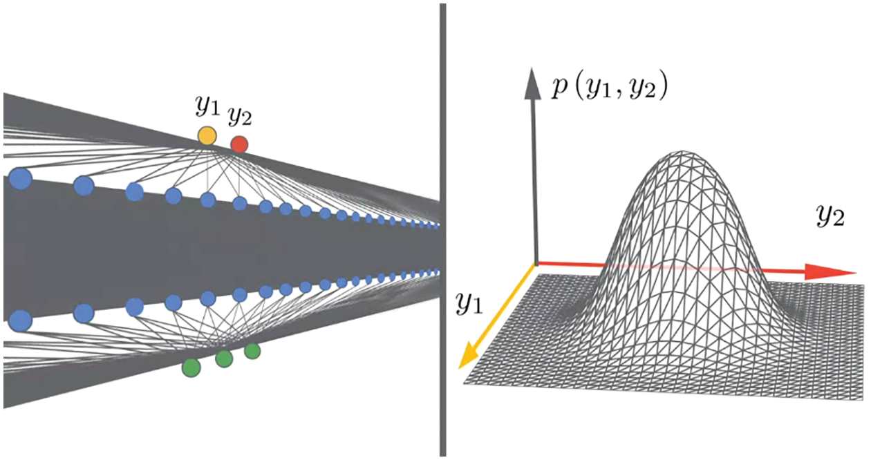
Figure 148: Network with infinite width (left) and Gaussian distribution (Right) (Section 6.1, 14.2). “A number of recent results have shown that DNNs that are allowed to become infinitely wide converge to another, simpler, class of models called Gaussian processes. In this limit, complicated phenomena (like Bayesian inference or gradient descent dynamics of a convolutional neural network) boil down to simple linear algebra equations. Insights from these infinitely wide networks frequently carry over to their finite counterparts. As such, infinite-width networks can be used as a lens to study deep learning, but also as useful models in their own right” [279] [231]. See Figures 60 and 61 for the motivation for networks with infinite width. (CC BY-SA 4.0, Wikipedia, version 03:51, 18 June 2022.)
The possibility of such attacks has been demonstrated in nearly every application domain of A.I., including computer vision, medical image processing, speech recognition and language processing. Numerous studies have demonstrated the ease with which hackers could, in principle, fool face- and object-recognition systems with specific minuscule changes to images, put inconspicuous stickers on a stop sign to make a self-driving car’s vision system mistake it for a yield sign or modify an audio signal so that it sounds like background music to a human but instructs a Siri or Alexa system to perform a silent command.
These potential vulnerabilities illustrate the ways in which current progress in A.I. is stymied by the barrier of meaning. Anyone who works with A.I. systems knows that behind the facade of humanlike visual abilities, linguistic fluency and game-playing prowess, these programs do not—in any humanlike way—understand the inputs they process or the outputs they produce. The lack of such understanding renders these programs susceptible to unexpected errors and undetectable attacks.
As the A.I. researcher Pedro Domingos noted in his book The Master Algorithm, ‘People worry that computers will get too smart and take over the world, but the real problem is that they’re too stupid and they’ve already taken over the world.’
Such barrier of meaning is also a barrier for AI to tackle human controversies; see Section 14.5. See also Section 14.1 on driverless cars not coming any time soon, which is related to the above barrier of meaning.
14.4 Threat to democracy and privacy
On the 2019 new-year day, The Guardian [67] not only reported the most recent breakthrough in AI research on the development of AlphaZero, a software possessing superhuman performance in several “immensely complex” games such as Go (see Section 13.5 on resurgence of AI and current state), they also reported another breakthrough as a more ominous warning on a “Power struggle” to preserve liberal democracies against authoritarian governments and criminals:
“The second great development of the last year makes bad outcomes much more likely. This is the much wider availability of powerful software and hardware. Although vast quantities of data and computing power are needed to train most neural nets, once trained a net can run on very cheap and simple hardware. This is often called the democratisation of technology but it is really the anarchisation of it. Democracies have means of enforcing decisions; anarchies have no means even of making them. The spread of these powers to authoritarian governments on the one hand and criminal networks on the other poses a double challenge to liberal democracies. Technology grants us new and almost unimaginable powers but at the same time it takes away some powers, and perhaps some understanding too, that we thought we would always possess.”
Nearly three years later, a report of a national poll of 2,200 adults in the U.S., released on 2021.11.15, indicated that three in four adults were concerned about the loss of privacy, “loss of trust in elections (57%), in threats to democracy (52%), and in loss of trust in institutions (56%). Additionally, 58% of respondents say it has contributed to the spread of misinformation” [396].

Figure 149: Deepfake images (Section 14.4.1). AI-generated portraits using Generative Adversarial Network (GAN) models. See also [397] [398], Chap. 8, “GAN Fingerprints in Face Image Synthesis.” (Images from ‘This Person Does Not Exist’ site.)
AI software available online helping to create videos that show someone said or did things that the person did not say or do represent a clear danger to democracy, as these deepfake videos could affect the outcome of an election, among other misdeeds, with risk to national security. Advances in machine learning have made deepfakes “ever more realistic and increasingly resistant to detection” [399]; see Figure 149. The authors of [400] concurred:
“Deepfake videos made with artificial intelligence can be a powerful force because they make it appear that someone did or said something that they never did, altering how the viewers see politicians, corporate executives, celebrities and other public figures. The tools necessary to make these videos are available online, with some people making celebrity mashups and one app offering to insert users’ faces into famous movie scenes.”
To be sure, deepfakes do have benefits in education, arts, and individual autonomy [399]. In education, deepfakes could be used to provide information to students in a more interesting manner. For example, deepfakes make it possible to “manufacture videos of historical figures speaking directly to students, giving an otherwise unappealing lecture a new lease on life”. In the arts, deepfake technology allowed to resurrect long dead actors for fresh roles in new movies. An example is a recent Star Wars movie with the deceased actress Carrie Fisher. In helping to maintain some personal autonomy, deepfake audio technology could help restore the ability to speak for a person suffered from some form of paralysis that prevents normal speaking.
On the other hand, the authors of [399] cited a long list of harmful uses of deepfakes, from harm to individuals or organizations (e.g., exploitation, sabotage), to harm to society (e.g., distortion of democratic discourse, manipulation of elections, eroding trust in institutions, exacerbating social division, undermining public safety, undermining diplomacy, jeopardizing national security, undermining journalism, crying deepfake news as liar’s dividend).333 See also [402] [403] [404] [405].
Researchers have been in a race to develop methods to detect deepfakes, a difficult technological challenge [406]. One method is to spot the subtle characteristics of how someone spoke to provide a basis to determine whether a video was true or fake [400]. But that method was not a top-five winner of the DeepFake Detection Challenge (DFDC) [407] organized in the period 2019-2020 by “The Partnership for AI, in collaboration with large companies including Facebook, Microsoft, and Amazon,” with a total prize money of one million dollars, divided among the top five winners, out of more than two thousand teams [408].
Human’s ability to detect of deepfakes compared well with the “leading model,” i.e., the DFCD top winner [408]. The results were “at odds with the commonly held view in media forensics that ordinary people have extremely limited ability to detect media manipulations” [408]; see Figure 150, where the width of a violin plot,334 at a given accuracy, represents the number of participants. In Col. 2 of Figure 150, the area of the blue violin above the leading model accuracy of 65% represents 82% of the participants, represented by the area of the whole violin. A crowd does have a collective accuracy comparable to (or for those who viewed at least 10 videos, better than) the leading model; see Cols. 5, 6, 7 in Figure 150.
While it is difficult to detect AI deepfakes, the MIT Media Lab DeepFake detection project advised to pay attention to the following eight facial features [411]:
(1) “Face. High-end DeepFake manipulations are almost always facial transformations.
(2) “Cheeks and forehead. Does the skin appear too smooth or too wrinkly? Is the agedness of the skin similar to the agedness of the hair and eyes? DeepFakes are often incongruent on some dimensions.
(3) “Eyes and eyebrows. Do shadows appear in places that you would expect? DeepFakes often fail to fully represent the natural physics of a scene.
(4) “Glasses. Is there any glare? Is there too much glare? Does the angle of the glare change when the person moves? Once again, DeepFakes often fail to fully represent the natural physics of lighting.
(5) “Facial hair or lack thereof. Does this facial hair look real? DeepFakes might add or remove a mustache, sideburns, or beard. But, DeepFakes often fail to make facial hair transformations fully natural.
(6) “Facial moles. Does the mole look real?
(7) Eye “blinking. Does the person blink enough or too much?
(8) “Size and color of the lips. Does the size and color match the rest of the person’s face?”
Figure 150: DeepFake detection (Section 14.4.1). Violin plots.
14.4.2 Facial recognition nightmare
“We’re all screwed” as a Clearview AI, startup company, uses deep learning to identify faces against a large database involving more than three billions photos collected from “Facebook, Youtube, Venmo and millions of other websites” [412]. Their software “could end your ability to walk down the street anonymously, and provided it to hundreds of law enforcement agencies”. More than 600 law enforcement agencies have started to use Clearview AI software to “help solve shoplifting, identity theft, credit card fraud, murder and child sexual exploitation cases”. On the other hand, the tool could be abused, such as identifying “activists at a protest or an attractive stranger on the subway, revealing not just their names but where they lived, what they did and whom they knew”. Some large cities such as San Francisco has banned to use of facial recognition by the police.
A breach of Clearview AI database occurred just a few weeks after the article by [412], an unforeseen, but not surprising, event [413]:
“Clearview AI, the controversial and secretive facial recognition company, recently experienced its first major data breach—a scary prospect considering the sheer amount and scope of personal information in its database, as well as the fact that access to it is supposed to be restricted to law enforcement agencies.”
The leaked documents showed that Clearview AI had a large range of customers, ranging from law-enforcement agencies (both domestic and internatinal), to large retail stores (Macy’s, Best Buy, Walmart). Experts describe Clearview AI’s plan to produce a publicly available face recognition app as “dangerous”. So we got screwed again.
There was a documented wrongful arrest by face-recognition algorithm that demonstrated racism, i.e., a bias toward people of color [414]. A detective showed the wrongful-arrest victim a photo that was clearly not the victim, and asked “Is this you?” to which the victim replied “You think all black men look alike?”
It is well known that AI has “propensity to replicate, reinforce or amplify harmful existing social biases” [415], such as racial bias [416] among others: “An early example arose in 2015, when a software engineer pointed out that Google’s image-recognition system had labeled his Black friends as ‘gorillas.’ Another example arose when Joy Buolamwini, an algorithmic fairness researcher at MIT, tried facial recognition on herself—and found that it wouldn’t recognize her, a Black woman, until she put a white mask over her face. These examples highlighted facial recognition’s failure to achieve another type of fairness: representational fairness” [417].335
A legal measure has been taken against gathering data for facial-recognition software. In May 2022, Clearview AI was slapped with a “$10 million for scraping UK faces from the web. That might not be the end of it”; in addition, “the firm was also ordered to delete all of the data it holds on UK citizens” [419].
There were more of such measures: “Earlier this year, Italian data protection authorities fined Clearview AI €20 million ($21 million) for breaching data protection rules. Authorities in Australia, Canada, France, and Germany have reached similar conclusions.
Even in the US, which does not have a federal data protection law, Clearview AI is facing increasing scrutiny. Earlier this month the ACLU won a major settlement that restricts Clearview from selling its database across the US to most businesses. In the state of Illinois, which has a law on biometric data, Clearview AI cannot sell access to its database to anyone, even the police, for five years” [419].
14.5 AI cannot tackle controversial human problems
If there was a barrier of meaning as described in Section 14.3, it is clear that there are many problems that AI could not be trained to solve since even humans do not agree on how to classify certain activities as offending or acceptable. It was written in [420] the following:
“Mr. Schroepfer—or Schrep, as he is known internally—is the person at Facebook leading the efforts to build the automated tools to sort through and erase the millions of [hate-speech] posts. But the task is Sisyphean, he acknowledged over the course of three interviews recently.
That’s because every time Mr. Schroepfer [Facebook’s Chief Technology Officer] and his more than 150 engineering specialists create A.I. solutions that flag and squelch noxious material, new and dubious posts that the A.I. systems have never seen before pop up—and are thus not caught. The task is made more difficult because “bad activity” is often in the eye of the beholder and humans, let alone machines, cannot agree on what that is.
“I don’t think I’m speaking out of turn to say that I’ve seen Schrep cry at work,” said Jocelyn Goldfein, a venture capitalist at Zetta Venture Partners who worked with him at Facebook.”
14.6 So what’s new? Learning to think like babies
Because of AI’s inability to understand (barrier of meaning) and to solve controversial human issues, a idea to tackle such problems is to start with baby steps in trying to teach AI to think like babies, as recounted by [321]:
“The problem is that these new algorithms are beginning to bump up against significant limitations. They need enormous amounts of data, only some kinds of data will do, and they’re not very good at generalizing from that data. Babies seem to learn much more general and powerful kinds of knowledge than AIs do, from much less and much messier data. In fact, human babies are the best learners in the universe. How do they do it? And could we get an AI to do the same?
First, there’s the issue of data. AIs need enormous amounts of it; they have to be trained on hundreds of millions of images or games.
Children, on the other hand, can learn new categories from just a small number of examples. A few storybook pictures can teach them not only about cats and dogs but jaguars and rhinos and unicorns.
AIs also need what computer scientists call “supervision.” In order to learn, they must be given a label for each image they “see” or a score for each move in a game. Baby data, by contrast, is largely unsupervised.
Even with a lot of supervised data, AIs can’t make the same kinds of generalizations that human children can. Their knowledge is much narrower and more limited, and they are easily fooled by what are called “adversarial examples.” For instance, an AI image recognition system will confidently say that a mixed-up jumble of pixels is a dog if the jumble happens to fit the right statistical pattern—a mistake a baby would never make.”
Regarding early stopping and generalization error in network training, see Remark 6.1 in Section 6.1. To make AIs into more robust and resilient learners, researchers are developing methods to build curiosity into AIs, instead of focusing on immediate rewards.
Figure 151: Lack of transparency and irreproducibility (Section 14.7). The table shows many missing pieces of information for the three networks—Lesion, Breast, and Case models—used to detect breast cancer. Learning rate, Section 6.2. Learning-rate schedule, Section 6.3.1, Figure 65 in Section 6.3.5. SGD with momentum, Section 6.3.2 and Remark 6.5. Adam algorithm, Section 6.5.6. Batch size, Sections 6.3.1 and 6.3.5. Epoch, Footnote 145. [421]. (Figure reproduced with permission of the authors).
14.7 Lack of transparency and irreproducibility of results
For “multiple years now”, there have been articles on deep learning that looked more like a promotion/advertisement for newly developed AI technologies, rather than scientific papers in the traditional sense that published results should be replicable and verifiable [422]. But it was only on 2020 Oct 14 that many scientists [421] had enough and protested the lack of transparency in AI research in a “damning” article in Nature, a major scientific journal.
“We couldn’t take it anymore,” says Benjamin Haibe-Kains, the lead author of the response, who studies computational genomics at the University of Toronto. “It’s not about this study in particular—it’s a trend we’ve been witnessing for multiple years now that has started to really bother us.” [422]
The particular contentious study was published by the Google-Health authors of [423] on the use of AI in medical imaging to detect breast cancer. But these authors of [423] provided so little information about their code and how it was tested that their article read more like a “promotion of proprietary tech” than a scientific paper. Figure 151 shows the missing pieces of crucial information to reproduce the results. A question would immediately come to mind: Why would a reputable journal like Nature accept such a paper? Was the review rigorous enough?
“When we saw that paper from Google, we realized that it was yet another example of a very high-profile journal publishing a very exciting study that has nothing to do with science,” Haibe-Kains says. “It’s more an advertisement for cool technology. We can’t really do anything with it.” [422]
According to [421], even though McKinney et al [423] stated that “all experiments and implementation details were described in sufficient detail in the supplementary methods section of their Article to ‘support replication with non-proprietary libraries’,” that was a subjective statement, and replicating their results would be a difficult task, since such textual description can hide a high level of complexity of the code, and nuances in the computer code can have large effects in the training and evaluation results.
“AI is feeling the heat for several reasons. For a start, it is a newcomer. It has only really become an experimental science in the past decade, says Joelle Pineau, a computer scientist at Facebook AI Research and McGill University, who coauthored the complaint. ‘It used to be theoretical, but more and more we are running experiments,’ she says. ‘And our dedication to sound methodology is lagging behind the ambition of our experiments.’ ” [422]
No progress in science could be made if results were not verifiable and replicable by independent researchers.
Oh, one more thing: “A.I. Is Making it Easier to Kill (You). Here’s How,” New York Times Documentaries, 2019.12.13 (Original website) (Youtube).
And getting better at it every day, e.g., by using “a suite of artificial intelligence-driven systems that will be able to control networked ‘loyal wingman’ type drones and fully autonomous unmanned combat air vehicles” [424]; see also “Collaborative Operations in Denied Environment (CODE) Phase 2 Concept Video” (Youtube).
1See also the Midjourney Showcase, Internet archived on 2022.09.07, the video Guide to MidJourney AI Art - How to get started FREE! and several other Midjourney tutorial videos on Youtube.
2Their goal was of course to discover fast multiplication algorithms for matrices of arbitrarily large size. See also “Discovering novel algorithms with AlphaTensor,” DeepMind, 2022.10.05, Internet archive.
3Tensors are not matrices; other concepts are summation convention on repeated indices, chain rule, and matrix index convention for natural conversion from component form to matrix (and then tensor) form. See Section 4.2 on Matrix notation.
4See the review papers on deep learning, e.g., [12] [13] [14] [15] [16] [17] [18], many of which did not provide extensive discussion on applications, particularly on computational mechanics, such as in the present review paper.
5An example of a confusing point for first-time learners with knowledge of electrical circuits, hydraulics, or (biological) computational neuroscience [19] would be the interpretation of the arrows in an artificial neural network such as those in Figure 7 and Figure 8: Would these arrows represent real physical flows (electron flow, fluid flow, etc.)? No, they represent function mapping (or information passing); see Section 4.3.1 on Graphical representation. Even a tutorial such as [20] would follow the same format as many other papers, and while alluding to the human brain in their Figure 2 (which is the equivalent of Figure 8 below), did not explain the meaning of the arrows.
6Particularly the top-down approach for both feedforward network (Section 4) and back propagation (Section 5).
7It took five years from the publication of Rumelhart et al. 1986 [22] to the paper by Ghaboussi et al. 1991 [23], in which backpropagation (Section 5) was applied. It took more than twenty years from the publication of Long Short-Term Memory (LSTM) units in [24] to the two recent papers [25] and [26], which are reviewed in detail here, and where recurrent neural networks (RNNs, Section 7) with LSTM units (Section 7.2) were applied, even though there were some early works on application of RNNs (without LSTM units) in civil / mechanical engineering such as [27] [28] [29] [30]. But already, “fully attentional Transformer” was proposed to render “intricately constructed LSTM” unnecessary [31]. Most modern networks use the default rectified linear function (ReLU)–which was introduced in computational neuroscience since at least before [32] and [19], and then adopted in computer science beginning with [33] and [34]–instead of the traditional sigmoid function dated since the mid 1970s with [35], but yet many newer activation functions continue to appear regularly, aiming at improving accuracy and efficiency over previous activation functions, e.g., [36], [37]. In computational mechanics, by the beginning of 2019, there has not yet widespread use of ReLU activation function, even though ReLU was mentioned in [38], where the sigmoid function was actually employed to obtain the results (Section 10). See also Section 13 on Historical perspective.
8It would be interesting to investigate on how the adjusted integration weights using the method in [38] would affect the stability of an element stiffness matrix with reduced integration (even in the absence of locking) and the superconvergence of the strains / stresses at the Barlow sampling points. See, e.g., [39], p. 499. The optimal locations of these strain / stress sampling points do not depend on the integration weights, but only on the degree of the interpolation polynomials; see [40] [41]. “The Gauss points corresponding to reduced integration are the Barlow points (Barlow, 1976) at which the strains are most accurately predicted if the elements are well-shaped” [42].
9It is only a coincidence that (1) Hochreiter (1997), the first author in [24], which was the original paper on the widely used and highly successful Long Short-Term Memory (LSTM) unit, is on the faculty at Johannes Kepler University (home institution of this paper’s author A.H.), and that (2) Ghaboussi (1991), the first author in [23], who was among the first researchers to apply fully-connected feedforward neural network to constitutive behavior in solid mechanics, was on the faculty at the University of Illinois at Urbana-Champaign (home institution of author L.V.Q.). See also [43], and for early applications of neural networks in other areas of mechanics, see e.g., [44], [45], [46].
10While in the long run an original website may be moved or even deleted, the same website captured on the Internet Archive (also known as Web Archive or Wayback Machine) remains there permanently.
11See also AlphaFold Protein Structure Database Internet archived as of 2022.09.02.
12The number of atoms in the observable universe is estimated at 1080. For a board game such as chess and Go, the number of possible sequences of moves is
13See [69] [6] [70] [71]. See also the film AlphaGo (2017), “an excellent and surprisingly touching documentary about one of the great recent triumphs of artificial intelligence, Google DeepMind’s victory over the champion Go player Lee Sedol” [72], and “AlphaGo versus Lee Sedol,” Wikipedia version 14:59, 3 September 2022.
14“ImageNet is an online database of millions of images, all labelled by hand. For any given word, such as “balloon” or “strawberry”, ImageNet contains several hundred images. The annual ImageNet contest encourages those in the field To compete and measure their progress in getting computers to recognise and label images automatically” [75]. See also [62] and [60], for a history of the development of ImageNet, which played a critical role in the resurgence of interest and research in AI by paving the way for the mentioned 2012 spectacular success in reducing the error rate in image recognition.
15For a report on the human image classification error rate of 5.1%, see [76] and [62], Table 10.
16Actually, the first success of deep learning occurred three years earlier in 2009 in speech recognition; see Section 2 regarding the historical perspective on the resurgence of AI.
18The authors of [13] cited this 2006 breakthrough paper by Hinton, Osindero & Teh in their reference no.32 with the mention “This paper introduced a novel and effective way of training very deep neural networks by pre-training one hidden layer at a time using the unsupervised learning procedure for restricted Boltzmann machines (RBMs).” A few years later, it was found out that RBMs were not necessary to train deep networks, as it was sufficient to use rectified linear units (ReLUs) as active functions ([79], interview with Y. Bengio); see also Section 4.4.2 on active functions. For this reason, we are not reviewing RBMs here.
19Intensive Care Unit.
20Food and Drug Administration.
21At video time 1:51. In less than a year, this 2018 April TED talk had more than two million views as of 2019 March.
22See Footnote 18 for the names of these three scientists.
23“The World Health Organization declares COVID-19 a pandemic” on 2020 Mar 11, CDC Museum COVID-19 Timeline, Internet archive 2022.06.02.
24Krisher T., Teslas with Autopilot a step closer to recall after wrecks, Associated Press, 2022.06.10.
25We thank Kerem Uguz for informing the senior author LVQ about Mathpix.
26Mathpix Snip “misunderstood” that the top horizontal line was part of a fraction, and upon correction of this “misunderstanding” and font-size adjustment yielded the equation image shown in Eq. (2).
27We are only concerned with NNs, not SVMs, in the present paper.
28References to books are accompanied with page numbers for specific information cited here so readers don’t waste time to wade through an 800-page book to look for such information.
29Network depth and size are discussed in Section 4.6.1. An example of a shallow network with one hidden layer can be found in Section 12.4 on nonlinear-manifold model-order reduction applied to fluid mechanics.
30See, e.g., [78], p. 5, p. 8, p. 14.
31For more on Support Vector Machine (SVM), see [78], p. 137. In the early 1990s, SVM displaced neural networks with backpropagation as a better method for the machine-learning community ([79], interview with G. Hinton). The resurgence of AI due to advances in deep learning started with the seminal paper [86], in which the authors demonstrated via numerical experiments that MLN network was better than SVM in terms of error in the handwriting-recognition benchmark test using the MNIST handwritten digit database, which contains “a training set of 60,000 examples, and a test set of 10,000 examples.” But kernel methods studied for the development of SVM have now been used in connection with networks with infinite width to understand how deep learning works; see Section 8 on “Kernel machines” and Section 14.2 on “Lack of understanding.”
33The neurons are the computing units, and the synapses the memory instead of grouping the computing units into a central processing unit (CPU), separated from the memory, and connect the CPU and the memory via a bus, which creates a communication bottleneck, like the brain, each neuron in the TrueNorth chip has its own synapses (local memory).
34In [20], there was only a reference to [87], but not to [88]. It is likely that the authors of [20] were not aware of [88], and thus an intersection between neuromorphic computing and deep learning.
35MLN is also called MultiLayer Perceptron (MLP); see Footnote 32.
36The quadrature weights at integration points are not to be confused with the network weights in a MLN network.
37See Section 6 on “Network training, optimization methods”.
38For the definition of training set and test set, see Section 6.1. Briefly, the training set is used to optimize the network parameters, while the test set is used to see how good the network with these optimized parameters can predict the targets of never-seen-before inputs.
39Information provided by author A. Oishi of [38] through a private communication to the authors on 2018 Nov 16.
40Porosity is the ratio of void volume over total volume. Permeability is a scaling factor, which when multiplied by the negative of the pressure gradient, and divided by the fluid dynamic viscosity, gives the fluid velocity in Darcy’s law, Eq. (409). The expression “dual-porosity dual-permeability poromechanics problem” used in [25], p. 340, could confuse first-time readers—especially those who are familiar with traditional reservoir simulation, e.g., in [92]—since dual porosity (also called “double porosity” in [89]) and dual permeability are two different models of naturally-fractured porous media; these two models for radionuclide transport around nuclear waste repository were studied in [93]. Further added to the confusion is that the dual-porosity model is more precisely called dual-porosity-single permeability model, whereas the dual-permeability model is called dual-porosity dual-permeability model [94], which has a different meaning than the one used in [25].
41See, e.g., [94], p. 295, Chap. 9 on “Advanced Topics: Fluid Flow in Fractured Reservoirs and Compositional Simulation”.
42At least at the beginning of Section 2 in [25].
43The LSTM variant with peephole connections is not the original LSTM cell (Section 7.2); see, e.g, [97]. The equations describing the LSTM unit in [25], whose authors never mentioned the word “peephole”, correspond to the original LSTM without peepholes. It was likely a mistake to use this figure in [25].
44The coordination number (Wikipedia version 20:43, 28 July 2020) is a concept originated from chemistry, signifying the number of bonds from the surrounding atoms to a central atom. In Figure 16 (a), the uranium borohydride U(BH4)4 complex (Wikipedia version 08:38, 12 March 2019) has 12 hydrogen atoms bonded to the central uranium atom.
45Briefly, dropout means to drop or to remove non-output units (neurons) from a base network, thus creating an ensemble of sub-networks (or models) to be trained for each example, and can also be considered as a way to add noise to inputs, particularly of hidden layers, to train the base network, thus making it more robust, since neural networks were known to be not robust to noise. Adding noise is also equivalent to increasing the size of the dataset for training, [78], p. 233, Section 7.4 on “Dataset augmentation”.
46From here on, if Eq. (5) is found a bit abstract at first reading, first-time learners could skip the remaining of this short Section 3 to begin reading Section 4, and come back later after reading through subsequent sections, particularly Section 13.2, to have an overview of the connection among seemingly separate topics.
47Eq. (5) is a reformulated version of Eq. (2.1) in [19], p. 46, and is similar to Eqs. (7.1)-(7.2) in [19], p. 233, Chapter “7 Network Models”.
48There is no physical flow here, only function mappings.
49Figure 2 in[20] is essentially the same as Figure 8.
51See, e.g., [78], p. 31, where a “vector” is a column matrix, and a “tensor” is an array with coefficients (elements) having more than two indices, e.g., Aijk. It is important to know the terminologies used in computer-science literature.
52The inputs x and the target (or labeled) outputs y are the data used to train the network, which produces the predicted (or approximated) output denoted by
53See, e.g., [107] [109] [110].
54See, e.g., [111], Footnote 11. For example,
55For example, the coefficient
56In [78], the column matrix (which is called “vector”)
57Soon, it will be seen in Eq. (26) that the function z is a linear combination of the network inputs
58The gradients of z will be used in the backpropagation algorithm in Section 5 to obtain the gradient of the error (or loss) function E to find the optimal weights that minimize E.
59To alleviate the notation, the predicted output
61In the review paper [12] addressing to computer-science experts, and dense with acronyms and jargon “foreign” to first-time learners, the authors mentioned “It is ironic that artificial NNs [neural networks] (ANNs) can help to better understand biological NNs (BNNs)”, and cited a 2012 paper that won an “image segmentation” contest in helping to construct a 3-D model of the “brain’s neurons and dendrites” from “electron microscopy images of stacks of thin slices of animal brains”.
62See Eq. (497) for the continuous temporal summation, counterpart of the discrete spatial summation in Eq. (26).
63It should be noted that the use of both
64Eq. (26) is a linear (additive) combination of inputs with possibly non-zero biases. An additive combination of inputs with zero bias, and a “multiplicative” combination of inputs of the form
65For the convenience in further reading, wherever possible, we use the same notation as in [78], p.xix.
66“In modern neural networks, The default recommendation is to use the rectified linear unit, or ReLU,” [78], p. 168.
67The notation
68A similar relation can be applied to define the Leaky ReLU in Eq. (40).
69In [78], p. 15, the authors cited the original papers [33] and [34], where ReLU was introduced in the context of image / object recognition, and [113], where the superiority of ReLU over hyperbolic-tangent units and sigmoidal units was demonstrated.
70See, e.g., [78], p. 219, and Section 13.3 on the history of active functions. See also Section 4.6 for a discussion of network size. The reason for less computational effort with ReLU is due to (1) it being an identity map for positive argument, (2) zero for negative argument, and (3) its first derivative being the Step (Heaviside) function as shown in Figure 24, and explained in Section 5 on Backpropagation.
71See, e.g., [19], p. 14, where ReLU was called the “half-wave rectification operation”, the meaning of which is explained above in Figure 26. The logistic sigmoid function (Figure 30) was also used in neuroscience since the 1950s.
72See Section 13.3.1 for a history of the sigmoid function, which dated back at least to 1974 in neuroscience.
73See the definition of image “predicate” or image “feature” in Section 13.2.1, and in particular Footnote 302.
75This one-layer network is not the Rosenblatt perceptron in Figure 132 due to the absence of the Heaviside function as activation function, and thus Section 4.5.1 is not the proof that the Rosenblatt perceptron cannot represent the XOR function. For such proof, see [121].
77See Section 13.2 on the history of the linear combination (weighted sum) of inputs with biases.
78In least-square linear regression, the normal equations are often presented in matrix form, starting from the errors (or residuals) at the data points, gathered in the matrix
79Our presentation is more detailed and more general than in [78], pp. 167-171, where there was no intuitive explanation of how the numbers were obtained, and where only the activation function ReLU was used.
80In general, the Heaviside function is not used as activation function since its gradient is zero, and thus would not work for gradient descent. But for this XOR problem without using gradient descent, the Heaviside function offers a workable solution as the rectified linear function.
81There are two viewpoints on the definition of depth, one based on the computational graph, and one based on the conceptual graph. From the computational-graph viewpoint, depth is the number of sequential instructions that must be executed in an architecture. From the conceptual-graph viewpoint, depth is the number of concept levels, going from simple concepts to more complex concepts. See also [78], p. 163, for the depth of fully-connected feedforward networks as the “length of the chain” in Eq. (18) and Eq. (23), which is the number of layers.
82There are several different network architectures. Convolutional neural networks (CNN) use sparse connections, have achieved great success in image recognition, and contributed to the burst of interest in deep learning since winning the ImageNet competion in 2012 by almost halving the image classification error rate; see [13, 12, 75]. Recurrent neural networks (RNN) are used to process a sequence of inputs to a system with changing states as in a dynamical system, to be discussed in Section 7. there are other networks with skip connections, in which information flows from layer
83A special type of deep network that went out of favor, then now back in favor, among the computer-vision and machine-learning communities after the spectacular success that ConvNet garnered at the 2012 ImageNet competition; see [13] [75] [74]. Since we are reviewing in detail some specific applications of deep networks to computational mechanics, we will not review ConvNet here, but focus on MultiLayer Neural (MLN)—also known as MultiLayer Perceptron (MLP)—networks.
84A network processing “unit” is also called a “neuron”.
86For other types of loss function, see, e.g., (1) Section “Loss functions” in “torch.nn—PyTorch Master Documentation” (Original website, Internet archive), and (2) Jah 2019, A Brief Overview of Loss Functions in Pytorch (Original website, Internet archive).
87There is an inconsistent use of notation in [78] that could cause confusion, e.g., in [78], Chap. 5, p. 104, Eq. (5.4), the notation
88In our notation, m is the dimension of the output array
89The simplified notation
90See, e.g., [78], p. 57. The notation
91A tilde is put on top of
93The normal (Gaussian) distribution of scalar random variable x, mean
96See also [78], p. 179 and p. 78, where the softmax function is used to stabilize against the underflow and overflow problem in numerical computation.
97Since the probability of x and y is
98See also [130], p. 115, version 1 of softmax function, i.e.,
99See [78], Section 6.5.4, p. 206, Algorithm 6.4.
101An epoch is when all examples in the dataset had been used in a training session of the optimization process. For a formal definition of “epoch”, see Section 6.3.1 on stochastic gradient descent (SGD) and Footnote 145.
104According to Google Scholar, [113] (2011) received 3,656 citations on 2019.10.13 and 8,815 citations on 2022.06.23, whereas [131] (2013) received 2,154 and 6,380 citations on these two respective dates.
105A “full batch” is a complete training set of examples; see Footnote 117.
106A minibatch is a random subset of the training set, which is called here the “full batch”; see Footnote 117.
107See “CIFAR-10”, Wikipedia, version 16:44, 14 October 2019.
108See also [78], p. 268, Section 8.1, “How learning differs from pure optimization”; that’s the classical thinking.
109See [134], p. 11, for a classification example using two methods: (1) linear models and least squares and (2) k-nearest neighbors. “The linear model makes huge assumptions about structure [high bias] and yields stable [low variance] but possibly inaccurate predictions [high training error]. The method of k-nearest neighbors makes very mild structural assumptions [low bias]: its predictions are often accurate [low training error] but can be unstable [high variance].” See also [130], p. 151, Figure 3.6.
110Andrew Ng suggested the following partitions. For small datasets having less than
111The word “estimate” is used here for the more general case of stochastic optimization with minibatches; see Section 6.3.1 on stochastic gradient descent and subsequent sections on stochastic algorithms. When deterministic optimization is used with the full batch of dataset, then the cost estimate is the same as the cost, i.e.,
112An epoch is when all examples in the dataset had been used in a training session of the optimization process. For a formal definition of “epoch”, see Section 6.3.1 on stochastic gradient descent (SGD) and Footnote 145.
113See also “Method for early stopping in a neural network”, StackExchange, 2018.03.05, Original website, Internet archive. [78], p. 287, also suggested to monitor the training learning curve to adjust the step length (learning rate).
114See Figure 151 in Section 14.7 on “Lack of transparency and irreproducibility of results” in recent deep-learning papers.
117A full batch contains all examples in the training set. There is a confusion in the use of the word “batch” in terminologies such as “batch optimization” or “batch gradient descent”, which are used to mean the full training set, and not a subset of the training set; see, e.g., [78], p. 271. Hence we explicitly use “full batch” for full training set, and mini-batch for a small subset of the training set.
118See, e.g., [80]. Noise is sometimes referred to as “discontinuities” as in [142]. See also the lecture video “Understanding mini-batch gradient descent,” at time 1:20, by Andrew Ng on Coursera website.
119In [78], a discussion on line search methods, however brief, was completely bypassed to focus on stochastic gradient-descent methods with learning-rate tuning and scheduling, such as AdaGrad, Adam, etc. Ironically, it is disconcerting to see these authors, who made important contributions to deep learning, thus helping thawing the last “AI winter”, regard with skepticism “most guidance” on learning-rate selection; see [78], p. 287, and Section 6.3. Since then, fully automatic stochastic line-search methods, without tuning runs, have been developed, apparently starting with [147]. In the abstract of [142], where an interesting method using only gradients, without function evaluations, was presented, one reads “Due to discontinuities induced by mini-batch sampling, [line searches] have largely fallen out of favor”.
120Or equivalently, the descent direction
121See, e.g., [139], p. 31, for the implementable algorithm, with the assumption that the cost function was convex. Convexity is, however, not needed for this algorithm to work; only unimodality is needed. A unimodal function has a unique minimum, and is decreasing on the left of the minimum, and increasing on the right of the minimum. Convex functions are necessarily unimodal, but not vice versa. Convexity is a particular case of unimodality. See also [148], p. 216, on Golden section search as infinite Fibonacci search and curve fitting line-search methods.
122See [149], p. 29, for this assertion, without examples. An example of non-existent minimizing step length
123The book [154] was cited in [139], p. 33, but not the papers [150] and [154]b, where Goldstein’s rule was explicitly presented in the form: Step length
125See [149], p. 55, and [156], p. 256, where the equality
126See [139], p. 36, Algorithm 36.
127As of 2022.07.09, [151] was cited 2301 times in various publications (books, papers) according to Google Scholar, and 1028 times in archival journal papers according to Web of Science. There are references that mention the name Armijo, but without referring to the original paper [151], such as [157], clearly indicating that Armijo’s rule is a classic, just like there is no need to refer to Newton’s original work for Newton’s method.
128All of these stochastic optimization methods are considered as part of a broader class known as derivative-free optimization methods [160].
129[156], p. 491, called the constructive technique in Eq. (125) to obtain the step length
130See also [157], p. 34, [148], p. 230.
132To satisfy the condition in Eq. (121), the descent direction
133The inequality in Eq. (128) leads to linear convergence in the sense that
134A narrow valley with the minimizer
135See, e.g., [149], p. 35, and [78], p. 302, where both cited the Levenberg-Marquardt algorithm as the first to use regularized Hessian.
136As of 2022.07.09, [152] was cited 1336 times in various publications (books, papers) according to Google Scholar, and 559 times in archival journal papers according to Web of Science.
137The authors of [140] and [141] may not be aware that Goldstein’s rule appeared before Armijo’s rule, as they cited Goldstein’s 1967 book [154], instead of Goldstein’s 1965 paper [150], and referred often to Polak (1971) [139], even though it was written in [139], p. 32, that a “step size rule [Eq. (124)] probably first introduced by Goldstein (1967) [154]” was used in an algorithm. See also Footnote 123.
138An earlier version of the 2017 paper [143] is the 2015 preprint [147].
139See [78], p. 271, about this terminology confusion. The authors of [80] used “stochastic” optimization to mean optimization using random “minibatches” of examples, and “batch” optimization to mean optimization using “full batch” or full training set of examples.
140The authors of [162] only cited [163] for a brief mention of “simulated annealing” as an example of “heuristic optimizers”, with no discussion, and no connection to step length decay. See also Remark 6.10 on “Metaheuristics”.
141The authors of [162] only cited [56] in passing, without reviewing AdamW, which was not even mentioned.
142The authors of [80] only cited Armijo (1966) [151] once for a pseudocode using line search.
143See, e.g., [80]–in which there was a short bio of Robbins, the first author of [167]–and [162] [144].
144As of 2010.04.30, the ImageNet database contained more than 14 million images; see Original website, Internet archive, Figure 3 and Footnote 14. There is a slight inconsistency in notation in [78], where on p. 148, 𝓂 and 𝓂' denote the number of examples in the training set and in the minibatch, respectively, whereas on p. 274, 𝓂 denote the number of examples in a minibatch. In our notation, 𝓂 is the dimension of the output array 𝓎, whereas 𝗆 (in a different font) is the minibatch size; see Footnote 88. In theory, we write
145An epoch, or training session, τ is explicitly defined here as when the minibatches as generated in Eqs. (135)-(137) covered the whole dataset. In [78], the first time the word “epoch” appeared was in Figure 7.3 caption, p. 239, where it was defined as a “training iteration”, but there was no explicit definition of “epoch” (when it started and when it ended), except indirectly as a “training pass through the dataset”, p. 274. See Figure 151 in Section 14.7 on “Lack of transparency and irreproducibility of results” in recent deep-learning papers.
146See also [78], p. 286, Algorigthm 8.1; [80], p. 243, Algorithm 4.1.
147See Figure 151 in Section 14.7 on “Lack of transparency and irreproducibility of results” in recent deep-learning papers.
148Often called by the more colloquial “heavy ball” method; see Remark 6.6.
149Sometimes referred to as Nesterov’s Accelerated Gradient (NAG) in the deep-learning literature.
150A nice animation of various optimizers (SGD, SGD with momentum, AdaGrad, AdaDelta, RMSProp) can be found in S. Ruder, ‘An overview of gradient descent optimization algorithms’, updated on 2018.09.02 (Original website).
151See also Section 6.5.3 on time series and exponential smoothing.
152Polyak (1964) [3]’s English version appeared before 1979, as cited [173], where a similar classical dynamics of a “small heavy sphere” or heavy point mass was used to develop an iterative method to solve nonlinear systems. There, the name Polyak was spelled as “Poljak” as in the Russian version. The earliest citing of the Russian version, with the spelling “Poljak” was in [156] and in [174], but the terminology “small heavy sphere” was not used. See also [171], p. 104 and p. 481, where the Russian version of [3] was cited.
153See [180], p. 159, p. 115, and [171], p. 104, respectively. The name “Polyak” was spelled as “Poljak” before 1990, [171], p. 481, and sometimes as “Polyack”, [169]. See also [181].
154See, e.g., [171], p. 104, [180], p. 115, [169], [181].
155Or the “Times Square Ball”, Wikipedia, version 05:17, 29 December 2019.
156Reference [50] cannot be found from the Web of Science as of 2020.03.18, perhaps because it was in Russian, as indicated in Ref. [35] in [51], p. 582, where Nesterov’s 2004 monograph was Ref. [39].
157A function
158The last two values did not belong to the sequence , with k being integers, since
159The Avant Garde font † is used to avoid confusion with t, the time variable used in relation to recurrent neural networks; see Section 7 on “Dynamics, sequential data, sequence modeling”, and Section 13.2.2 on “Dynamics, time dependence, Volterra series”. Many papers on deep-learning optimizers used t as global iteration counter, which is denoted by j here; see, e.g., [182], [56].
160See [78], p. 287, where it was suggested that †c in Eq. (147) would be “set to the number of iterations required to make a few hundred passes through the training set,” and ∈†c “should be set to roughly 1 percent the value of
161See [182], p. 3, below Algorithm 1 and just below the equation labeled “(Sgd)”. After, say, 400 global iterations, i.e., † = j = 400, then ∈400 = 5%∈0 according to Eq. (149), and
162Eq. (155) are called the “stepsize requirements” in [80], and “sufficient condition for convergence” in [78], p. 287, and in [184]. Robbins & Monro (1951b) [49] were concerned with solving
163See, e.g., [185], p. 36, Eq. (2.8.3).
164Eq. (168) possesses a simplicity elegance compared to the expression
165In [186] and [164], the fluctuation factor was expressed, in original notation, as
166See Figure 151 in Section 14.7 on “Lack of transparency and irreproducibility of results” in recent deep-learning papers.
168“In metallurgy and materials science, annealing is a heat treatment that alters the physical and sometimes chemical properties of a material to increase its ductility and reduce its hardness, making it more workable. It involves heating a material above its recrystallization temperature, maintaining a suitable temperature for a suitable amount of time, and then allow slow cooling.” Wikepedia, ‘Annealing (metallurgy)’, Version 11:06, 26 November 2019. The name “simulated annealing” came from the highly cited paper [163], which received more than 20,000 citations on Web of Science and more than 40,000 citations on Google Scholar as of 2020.01.17. See also Remark 6.10 on “Metaheuristics”.
167See Figure 151 in Section 14.7 on “Lack of transparency and irreproducibility of results” in recent deep-learning papers.
169In original notation used in [185], p. 53, Eq. (3.5.10) reads as
170See also “Langevin equation”, Wikipedia, version 17:40, 3 December 2019.
171For first-time learners, here a guide for further reading on a derivation of Eq. (179). It is better to follow the book [189], rather than Coffey’s 1985 long review paper, cited for equation
173Situations favoring a nonzero initialization of weights are explained in [78], p. 297.
175Reference [170] introduced the Adam algorithm in 2014, received 34,535 citations on 2019.12.11, after 5 years, and a whopping 112,797 citations on 2022.07.11, after an additional period of more than 2.5 years later, according to Google Scholar.
176In lines 12-13 of Algorithm 5, use Eq. (183), but replacing scalar learning rate
177The uppercase letter
180AdaDelta and RMSProp used the first form of Eq. (200), with Δ outside the square root, whereas AdaGrad and Adam used the second part, with Δ inside the square root. AMSGrad, Nostalgic Adam, AdamX did not use Δ, i.e., set
181There are no symbols similar to the Hadamard operator symbol ⊙ for other operations such as square root, addition, and division, as implied in Eq. (200), so there is no need to use the symbol ⊙ just for multiplication.
182As of 2019.11.28, [52] was cited 5,385 times on Google Scholars, and 1,615 times on Web of Science. By 2022.07.11, [52] was cited 10,431 times on Google Scholars, and 3,871 times on Web of Science.
183See [54]. For example, compare the sequence to the sequence . The authors of [78], p. 299, mistakenly stated “The parameters with the largest partial derivative of the loss have a correspondingly rapid decrease in their learning rate, while parameters with small partial derivatives have a relatively small decrease in their learning rate.”
184It was stated in [54]: “progress along each dimension evens out over time. This is very beneficial for training deep neural networks since the scale of the gradients in each layer is often different by several orders of magnitude, so the optimal Learning rate should take that into account.” Such observation made more sense than saying “The net effect is greater progress in the more gently sloped directions of parameter space” as did the authors of [78], p. 299, who referred to AdaDelta in Section 8.5.4, p. 302, through the work of other authors, but might not read [54].
185We thank Lawrence Aitchison for informing us about these references; see also [168].
187Almost all authors, e.g., [80] [55] [162], attributed RMSProp to Ref. [53], except for Ref. [78], where only Hinton’s 2012 Coursera lecture was referred to. Tieleman was Hinton’s student; see the video and the lecture notes in [53], where Tieleman’s contribution was noted as unpublished. The authors of [162] indicated that both RMSProp and AdaDelta (next section) were developed independently at about the same time to fix problems in AdaGrad.
188Neither [162], nor [80], nor [78], p. 299, provided the meaning of the acronym RMSProp, which stands for “Root Mean Square Propagation”.
189In spite of the nice features in AdaDelta, neither [78], nor [80], nor [162], had a review of AdaDelta, except for citing [54], even though the authors of [78], p. 302, wrote: “While the results suggest that the family of algorithms with adaptive learning rates (represented by RMSProp and AdaDelta) performed fairly robustly, no single best algorithm has emerged,” and “Currently, the most popular optimization algorithms actively in use include SGD, SGD with momentum, RMSProp, RMSProp with momentum, AdaDelta, and Adam.” The authors of [80], p. 286, did not follow the historical development, briefly reviewed RMSProp, then cited in passing references for AdaDelta and Adam, and then mentioned the “popular AdaGrad algorithm” as a “member of this family”; readers would lose sight of the gradual progress made starting from AdaGrad, to RMSProp, AdaDelta, then Adam, and to the recent AdamW in [56], among others, alternating with pitfalls revealed and subsequent fixes, and then more pitfalls revealed and more fixes.
190A random process is stationary when its mean and standard deviation stay constant over time.
191Sixth International Conference on Learning Representations (Website).
192The authors of [182] distinguished the step size
193To write this term in the notation used in[182], Theorem 4 and Corollary 1, simply make the following changes in notation:
194The notation “G” is clearly mnemonic for “gradient”, and the uppercase is used to designate upperbound.
195See also [183], p. 4, Lemma 2.4.
196See a description of the NMIST dataset in Section 5.3 on “Vanishing and exploding gradients”. For the difference between logistic regression and neural network, see, e.g., [208], Raschka, “Machine Learning FAQ: What is the relation between Logistic Regression and Neural Networks and when to use which?” Original website, Internet archive. See also [78], p. 200, Figure 6.8b, for the computational graph of Logistic Regression (one-layer network).
198See [55], p. 4, Section 3.3 “Adaptivity can overfit”.
199See [78], p. 107, regarding training error and test (generalization) error. “The ability to perform well on previously unobserved inputs is called generalization.”
200See, e.g., [210], where [55] was not referred to directly, but through a reference to [164], in which there was a reference to [55].
201See [78], p. 107, Section 5.2 on “Capacity, overfitting and underfitting”, and p. 115 provides a good explanation and motivation for regularization, as in Gupta 2017, ‘Deep Learning: Overfitting’, 2017.02.12, Original website, Internet archive.
202It is not until Section 4.7 in [144] that this version is presented for the general descent of nonconvex case, whereas the pseudocode in their Algorithm 1 at the beginning of their paper, and referred to in Section 4.5, was restricted to steepest descent for convex case.
203See [144], p. 7, below Eq. (2.4).
204Based on our private communications with the authors of [144] on 2019.11.16.
205The Armijo line search itself is 1st order; see Section 6.2 on full-batch deterministic optimization.
206See Step 2 of Algorithm 1 in [145].
207Per our private correspondence as of 2019.12.18.
208The state-space representation of time-continuous LTI-systems in control theory, see, e.g., Chapter 3 of [213], “State Variables and the State Space Description of Dynamic Systems” is typically written as
209See Section 13.2.2 on “Dynamic, time dependence, Volterra series”.
210See the general time-continuous neural network with a continuous delay described by Eq. (514).
211We can regard the trapezoidal rule as a combination of Euler’s explicit and implicit methods. The explicit Euler method approximates time-integrals by means of rates (and inputs) at the beginning of a time step. The next state (at the end of a time step) is obtained from previous state and the previous input as
212Though the elements
213cf. [78], p. 371, Figure 10.5.
214See PyTorch documentation: Recurrent layers, Original website (Internet archive)
215See TensorFlow API: TensorFlow Core r1.14: tf.keras.layers.SimpleRNN, Original website (Internet archive)
216For this reason,
217Such neural network is universal, i.e., any function computable by a Turing machine can be computed by an RNN of finite size, see [78], p. 368.
219The cell state is denoted with the variable s in [78], p. 399, Eq. (10.41).
221 Autoencoders are a special kind of encoder-decoder networks, which are trained to reproduce the input sequence, see Section 12.4.3.
222For more details on different types of RNNs, see, e.g., [78], p. 385, Section 10.4 “Encoder-decoder sequence-to-sequence architectures.”
226Unlike the use of notation in [31], we use different symbols for the arguments of the scaled dot-product attention function, Eq. (312), and those of the multi-head attention, Eq. (314), to emphasize their distinct dimensions.
227Eq. (318) is meant to reflect the idea off position-wise computations of the second sub-layer, since single vectors
228A cloze is “a form of written examination in which candidates are required to provide words that have been omitted from sentences, thereby demonstrating their knowledge and comprehension of the text”, see Wiktionary version 11:23, 2 January 2022.
229The stiffness matrix in the displacement finite element method is a Gram matrix.
230See Eq. (6), p. 346, in [237].
231Eq. (342)1, and Eqs. (343)1,2 were given as Eq. (5.46), Eq. (5.47), and Eq. (5.45), respectively, in [238], pp. 168-169, where the basis functions
232See [238], Eq. (3.41), p. 61, which is in Section 3.4.1 on “Ridge regression,” which “shrinks the regression coefficients by imposing a penalty on them.” Here the penalty is imposed on the kernel-induced norm of f, i.e.,
233In classical regularization, the loss function (1st term) in Eq. (344) is called the “empirical risk” and the penalty term (2nd term) the “stabilizer” [239].
235See also [238], p. 169, Eq. (5.50), and p. 185.
236A succinct introduction to Hilbert space and the Riesz Representation theorem, with detailed proofs, starting from the basic definitions, can be found in [243].
237In [130], p. 305, the kernel
238It is possible to define the Laplacian kernel in Eq. (359)
239Non-Gaussian processes, such as in [245] [246], are also important, but more advanced, and thus beyond the scope of the present review. See also the Gaussian-Process Summer-School videos (Youtube) 2019 and 2021. We thank David Duvenaud for noting that we did not review non-Gaussian processes.
240The “precision” is the inverse of the variance, i.e.,
241That the Gram matrix is positive semidefinite should be familiar with practitioners of the finite element method, in which the Gram matrix is the stiffness matrix (for elliptic differential operators), and is positive semidefinite before applying the essential boundary conditions.
242See, e.g., [234], p. 16, [130], p. 87, [247], p. 4. The authors of [234], in their Appendix A.2, p. 200, referred to [248] “sec. 9.3” for the derivation of Eqs. (378)-(379), but there were several sections numbered “9.3” in [248]; the correct referencing should be [248], Chapter XIII “More on distributions,” Sec. 9.3 “Marginal distributions and conditional distributions,” p. 427.
243The Matlab code for generating Figures 87 and 88 was provided courtesy of David Duvenaud. On line 25 of the code, the noise variance
245See this link for the latest Google Trends results corresponding to Figure 91.
246In the context of DL, multi-dimensional arrays are also referred to a tensors, although the data often lacks the defining properties of tensors as algebraic objects. The software framework TensorFlow even reflects that by its name.
247See Google’s announcement of TPUs [251].
248Recall that the ‘exa’-prefix translates into a factor of 1 × 10¹⁸. For comparison, Nvidia’s latest H100 GPU-based accelerator has a half-precision floating point (bfloat16) performance of 1 petaflops.
249See this blog post on the history of PyTorch [254] and the YouTube talk of Yann LeCun, PyTorch co-creator Sousmith Chintala, Meta’s PyTorch lead Lin Qiao and Meta’s CTO Mike Schroepfer [255].
250GPU-computing and automatic differentiation are by no means new to scientific computing not least in the field of computational mechanics. Project Chrono (see Original website), for instance, is well known for its support of GPU-computing in problems of flexible multi-body and particle systems. The general purpose finite-element code Netgen/NGSolve [265] (see Original website) offers a great degree of flexibility owing to its automatic differentiation capabilities. Well-established commercial codes, on the other hand, are often built on a comparatively old codebase, which dates back to times before the advent of GPU-computing.
251For incompressible flow past a cylinder, the computational domain of dimension
252See Section Working with different backends. See also [269].
253“All you need is to import GenericSolver from neurodiffeq.solvers, and Generator3D from neurodiffeq.generators. The catch is that currently there is no reparametrization defined in neurodiffeq.conditions to satisfy 3D boundary conditions,” which can be hacked into the loss function “by either adding another element in your equation system or overwriting the additional_loss method of GenericSolve.” Private communication with a developer of NeuroDiffEq on 2022.10.08.
254There are many comparisons of Julia versus Python on the web; one is Julia vs Python: Which is Best to Learn First?, by By Zulie Rane on 2022.02.05, updated on 2022.10.01.
255The 2019 paper [282] was a merger of a two-part preprint [292] [293].
256See, e.g., [39], p.61, Section “3.5 Isoparametric form” and p.170, Section “6.5 Mapping: Parametric forms.”
257Using Gauss-Legendre quadrature, p integration points integrate polynomials up to a degree of
258Conventional linear hexahedra are known to suffer from locking, see, e.g., [39] Section “10.3.2 Locking,” which can be alleviated by “reduced integration,” i.e., using a single integration point (
259In fact, a somewhat ambiguous description of the random generation of elements was provided in [38]. On the one hand, the authors stated that a “…coordinates of nodes are changed using a uniform random number r …,” and did not distinguish the random numbers in Eq. (400) by subscripts. On the other hand, they noted that exaggerated distortion may occur if nodal coordinates of an element were changed independently, and introduced the constraints on the distortion mentioned above in that context. If the same random number r were used for all nodal coordinates, all elements generated would exhibit the same mode of distortion.
260For example, for a
261The authors of [38] used the squared-error loss function (Section 5.1.1) for the classification task, for which the softmax loss function can also be used, as discussed in Section 5.1.3.
262There was no indication in [38] on how these 5,000 elements were selected from the total of 10,000 elements, perhaps randomly.
263In contrast to the terminology of the present paper, in which “training set” and “validation set” are used (Section 6.1), the terms “training patterns” and “test patterns”, respectively, were used in [38]. The “test patterns” were used in the training process, since the authors of [38] “…terminated the training before the error for test patterns started to increase” (p.331). These “test patterns”, based on their use as stated, correspond to the elements of the validation set in the present paper, Figure 100. Technically, there was no test set in [38]; see Section 6.1.
264The first author of [38] provided the information on the activation function through a private communication to the authors on 2018 Nov 16. Their tests with the ReLU did not show improved performance (in terms of accuracy) as compared to the logistic sigmoid.
265Even though the squared-error loss function (Section 5.1.1) was used in [38], we also discuss the softmax loss function for classification tasks; see Section 5.1.3.
266Even though a reason for not using the entire set of 20000 elements was not given, it could be guessed that the authors of [38] would want the size of the training set and of the validation set to be the same as that in Method 1, Section 10.2. Moreover, even though details were not given, the selection of these 10,000 elements would likely be a random process.
267According to Figure 101, only 4868 out of in total 20000 elements generated belonged to Category B, for which
268No details on the normalization procedure were provided in the paper.
269The caption of Figure 10, if it were in Section 10.3.3, would begin with “Method 2, application phase” in parallel to the caption of Figure 100.
270See, e.g., [294] [295] [296].
271DEM = Discrete Element Method. FEM = Finite Element Method. See references in [25].
272RVEs are also referred to as representative elementary volumes (REVs) or, simply, unit cells.
273The subscript
278Recall that
279The authors of [26] did not have a validation dataset as defined in Section 6.1.
280“Hurst exponent”, Wikipedia, version 22:09, 30 October 2020.
281See pyMOR website https://pymor.org/.
282Note that the authors also published a second condensed, but otherwise similar version of their article, see [48].
283As opposed to the classical non-parametric case, in which all parameters are fixed, parametric methods aim at creating ROMs which account for (certain) parameters of the underlying governing equations to vary in some given range. Optimization of large-scale systems, for which repeated evaluations are computationally intractable, is a classical use-case for methods in parametric MOR, see Benner et al. [307].
284Mathematically, the dimensionality of linear subspace that ‘best’ approximates a nonlinear manifold is described by the Kolmogorov n-width, see, e.g., [308] for a formal definition.
285In solid mechanics, we typically deal with second-order ODEs, which can be converted into a system of first-order ODEs by including velocities in the state space. For this reason, we prefer to use the term ‘rate’ rather than ‘velocity’ of
286The tilde above the symbol for the residual function
287As the authors of [47] omitted a step-by-step derivation, we introduce it here for the sake of completeness.
288See [78], Chapter 14, p.493.
289In fact, linear decoder networks combined with MSE-loss are equivalent to the Principal Components Analysis (PCA) (see [78], p.494), which, in turn, is equivalent to the discrete variant of POD by means of singular value decomposition (see Remark 12.2).
290The authors of [47] did not provide further details.
291Note again that the step-by-step derivations of the ODEs in Eq. (477) were not given by the authors of [47], which is why we provide it in our review paper for the sake of clarity.
292The “Unassembled DEIM” (UDEIM) method proposed in [315] provides a partial remedy for that issue in the context of finite-element problems. In UDEIM, the algorithm is applied to the unassembled residual vector, i.e., the set of element residuals, which restricts the dependency among generalized coordinates to individual elements.
293“The Perceptron’s design was much like that of the modern neural net, except that it had only one layer with adjustable weights and thresholds, sandwiched between input and output layers” [77]. In the neuroscientific terminology that Rosenblatt (1958) [119] used, the input layer contains the sensory units, the middle (hidden) layer contains the “association units,” and the output layer contains the response units. Due to the difference in notation and due to “neurodynamics” as a new field for most readers, we provide here some markers that could help track down where Rosenblatt used linear combination of the inputs. Rosenblatt (1962) [2], p. 82, defined the “transmission function
294We were so thoroughly misled in thinking that the “Rosenblatt perceptron” was a single neuron that we were surprised to learn that Rosenblatt had built the Mark I computer with many neurons.
295Heaviside activation function, see Figure 132 for the case of one neuron.
296Weighted sum / voting (or linear combination) of inputs; see Eq. (488), Eq. (493), Eq. (494).
297The negative of the bias
298Refer to Figure 131. A synapse (meaning “junction”) is “a structure that permits a neuron (or nerve cell) to pass an electrical or chemical signal to another neuron”, and consists of three parts: the presynaptic part (which is an axon terminal of an upstream neuron from which the signal came), the gap called the synaptic cleft, and the postsynaptic part, located on a dendrite or on the neuron cell body (called the soma); [19], p. 6; “Synapse”, Wikipedia, version 16:33, 3 March 2019. A dendrite is a conduit for transmitting the electrochemical signal received from another neuron, and passing through a synapse located on that dendrite; “Dendrite”, Wikipedia, version 23:39, 15 April 2019. A synapse is thus an input point to a neuron in a biological neural network. An axon, or nerve fiber, is a “long, slender projection of a neuron, that conducts electrical impulses known as action potentials” away from the soma to the axon terminals, which are the presynaptic parts; “Axon terminal”, Wikipedia, version 18:13, 27 February 2019.
299See “Kirchhoff’s circuit laws”, Wikipedia, version 14:24, 1 May 2019.
300See, e.g., “Perceptron”, Wikipedia, version 13:11, 10 May 2019, and many other references.
301Of course, the notation
302See [78], p. 3. Another example of a feature is a piece of information about a patient for medical diagnostics. “For many tasks, it is difficult to know which features should be extracted.” For example, to detect cars, we can try to detect the wheels, but “it is difficult to describe exactly what a wheel looks like in terms of pixel values”, due to shadows, glares, objects obscuring parts of a wheel, etc.
306First equation, unnumbered, in [120]. That this equation was unnumbered also indicated that it would not be subsequently referred to (and hence perhaps not considered as important).
307See above Eq. (1) in [120].
308A search on the Web of Science on 2019.07.04 indicated that [119] received 2,346 citations, whereas [120] received 168 citations. A search on Google Books on the same day indicated that [2] received 21 citations.
309[19], p. 46. “The Volterra series is a model for non-linear behavior similar to the Taylor series. It differs from the Taylor series in its ability to capture ’memory’ effects. The Taylor series can be used for approximating the response of a nonlinear system to a given input if the output of this system depends strictly on the input at that particular time. In the Volterra series the output of the nonlinear system depends on the input to the system at all other times. This provides the ability to capture the ’memory’ effect of devices like capacitors and inductors. It has been applied in the fields of medicine (biomedical engineering) and biology, especially neuroscience. In mathematics, a Volterra series denotes a functional expansion of a dynamic, nonlinear, time-invariant functional,” in “Volterra series”, Wikipedia, version 12:49, 13 August 2018.
310Since the first two terms in the Volterra series coincide with the first two terms in the Wiener series; see [19], p. 46.
312See [19], p. 234, below Eq. (7.3).
313The negative of the bias
314In general, for
315See [19], p. 234, in original notation as
316See [19], p. 234, subsection “The Firing Rate”.
317Eq. (1) and Eq. (2) in [116].
318In original notation, Eq. (510) was written as
319In original notation, Eq. (512) was written as
321The “Square Nonlinearity (SQNL)” activation, having a shape similar to that of the hyperbolic tangent function, appeared in the article “Activation function” for the last time in version 22:00, 17 March 2021, and was was removed from the table of activation functions starting from version 18:13, 11 April 2021 with the comment “Remove SQLU since it has 0 citations; it needs to be broadly adopted to be in this list; Remove SQNL (also from the same author, and this also does not have broad adoption)”; see the article History.
322See [78], Chap. 8, “Optimization for training deep models”, p. 267.
323See Footnote 31 on how research on kernel methods (Section 8) for Support Vector Machines have been recently used in connection with networks with infinite width to understand how deep learning works (Section 14.2).
324We only want to point out the connection between backprop and AD, together with a recent review paper on AD, but will not review AD itself here.
325As of 2020.12.18, the COVID-19 pandemic was still raging across the entire United States.
326Private communication with Karel (Carl) Moons on 2021 Oct 28. In other words, only medical journals included in PROBAST would report Covid-19 models that cannot be beaten by models reported in non-medical journals, such as in [333], which was indeed not “fit for clinical use” to use the same phrase in [334].
327“In medical diagnosis, test sensitivity is the ability of a test to correctly identify those with the disease (true positive rate), whereas test specificity is the ability of the test to correctly identify those without the disease (true negative rate).” See “Sensitivity and specificity”, Wikipedia version 02:21, 22 February 2021. For the definition of “AUC” (Area Under the ROC Curve), with “ROC” abbreviating for “Receiver Operating characteristic Curve”, see “Classification: ROC Curve and AUC”, in “Machine Learning Crash Course”, Website. Internet archive.
328One author of the present article (LVQ), more than one year after the preprint of [333], still spit into a tube for Covid test instead of coughing into a phone.
329A ligand is “usually a molecule which produces a signal by binding to a site on a target protein,’ see “Ligand (biochemistry)”, Wikipedia, version 11:08, 8 December 2021.
330SEIR = Susceptible, Exposed, Infectious, Recovered; see “Compartmental models in epidemiology”, Wikipedia, version 15:44, 19 February 2022.
331Fundus is “the interior surface of the eye opposite the lens and includes the retina, optic disc, macula, fovea, and posterior pole” (Wikipedia, version 02:49, 7 January 2020). Fluorescein is an organic compound and fluorescent dye (Wikipedia, version 19:51, 6 January 2022). Angiography (angio- “blood vessel” + graphy “write, record”, Wikipedia, version 10:19, 2 February 2022) is a medical procedure to visualize the flow of blood (or other biological fluid) by injecting a dye and by using a special camera.
332S.J. Russell also appeared in the video “AI is making it easier...” mentioned at the end of this closure section.
333Watch also Danielle Citron’s 2019 TED talk “How deepfakes undermine truth and threaten democracy” [401].
334See the classic original paper [409], which was cited 1,554 times on Google Scholar as of 2022.08.24. See also [410] with Python code and resulting images on GitHub.
335See also [418] on a number of relevant AI ethical issues such as: “Who bears responsibility in the event of harm resulting from the use of an AI system; How can AI systems be prevented from reflecting existing discrimination, biases and social injustices based on their training data, thereby exacerbating them; How can the privacy of people be protected, given that personal data can be collected and analysed so easily by many.” Perhaps the toughest question is “Who should get to decide which moral intuitions, which values, should be embedded in algorithms?” [417].
336The landmark paper “Little (1974)” was not listed in the Web of Science database as of Nov 2018, using the search keywords [au=(little) and py=(1974) and ts=(brain)]. On the other hand, [au=(little) and ts=(The existence of persistent states in the brain)], i.e., the author’s last name and the full title of the paper, led to the 1995 collection of Little’s papers edited by Cabrera et al., in which ‘Little (1974)’was found.
337In a rather cryptic manner to outsiders, several computer-science papers refer to papers in the Computing Research Repository (CoRR) such as, e.g., “CoRR abs/1706.03762v5”, which means that the abstract of paper number “1706.03762v5” (version 5) can be accessed by prepending to “abs/1706.03762v5” the CoRR web address https://arxiv.org/ to form https://arxiv.org/abs/1706.03762v5, which can also be obtained via a web search of “abs/1706.03762v5”, and where the PDF of the paper can be downloaded. An equivalent reference is “arXiv preprint arXiv:1706.03762v5”, which may be clearer since more non-computer-science readers would have heard of the arXiv rather than the CoRR. Papers such as [31] use both types of references, which are also used in the present review paper so readers become familiar with both. To refer to the specific version 5, use “CoRR abs/1706.03762v5”; to refer to the latest version (which may be different from version 5), remove “v5” to use only “CoRR abs/1706.03762”.
338MLP = MultiLayer Perceptron.
341The total number of papers on the topic “cyberneti*” was 7,962 on 2020.04.15–as shown in Figure 154 obtained upon clicking on the “Citation Report” button in the Web of Science–and 8,991 on 2022.08.08. Since the distribution in Figure 154, the points made in the figure caption and in this section remain the same, there was no need to update the figure to its 2022.08.08 version.
342The number of categories has increased to 244 in the Web of Sciecne search on 2022.08.08, mentioned in Footnote 341, with the number of papers in Computer Science Cybernetics at 2,952, representing 32% of the 8,991 papers in this topic.
343These cybernetics conferences were called the Macy conferences, held during a short period from 1946 to 1953, and involved researchers from diverse fields: not just mathematics, physics, engineering, but also anthropology and physiology, [431], pp.2-3.
References
1. Rosenblatt, F. (1957). The perceptron: A perceiving and recognizing automaton. Technical report, Cornell University. Cornell University, Report No. 85-460-1. Project PARA, January. Internet archive. 1070, 1079, 1123, 1279, 1339 [Google Scholar]
2. Rosenblatt, F. (1962). Principles of neurodynamics: Perceptrons and the theory of brain mechanisms. Spartan Books. 1070, 1079, 1114, 1123, 1278, 1280, 1281, 1282, 1283, 1339 [Google Scholar]
3. Polyak, B. (1964). Some methods of speeding up the convergence of iteration methods. USSR Computational Mathematics and Mathematical Physics, 4(51–17. DOI 10.1016/0041-5553(64)90137-5. 1070, 1078, 1079, 1153, 1157, 1158, 1159 [Google Scholar] [CrossRef]
4. Roose, K. (2022). An A.I.-Generated PictureWon an Art Prize. Artists Aren’t Happy. New York Times, (Sep 2). Original website. 1074, 1075 [Google Scholar]
5. Jumper, J., Evans, R., Pritzel, A., Green, T., Figurnov, M., et al. (2021). Highly accurate protein structure prediction with AlphaFold. Nature, 596(7873583–589. 1076 [Google Scholar] [PubMed]
6. Silver, D., Huang, A., Maddison, C. J., Guez, A., Sifre, L., et al. (2016). Mastering the game of Go with deep neural networks and tree search. Nature, 529(7587484+. Original website. 1076, 1080, 1081 [Google Scholar] [PubMed]
7. Moyer, C. How Google’s AlphaGo Beat a GoWorld Champion. 2016 Mar 28, Original website. 1076 [Google Scholar]
8. Edwards, B. (2022). DeepMind breaks 50-year math record using AI; new record falls a week later. Ars Technica, (Oct 13). Original website, Internet archive. 1074 [Google Scholar]
9. Vu-Quoc, L., Humer, A. (2022). Deep learning applied to computational mechanics: A comprehensive review, state of the art, and the classics. arXiv:2212.08989. 1074 [Google Scholar]
10. Roose, K. (2023). Bing (Yes, Bing) Just Made Search Interesting Again. New York Times, (Feb 8). Original website. 1074 [Google Scholar]
11. Knight, W. (2023). Meet Bard, Google’s Answer to ChatGPT. WIRED, (Feb 6). Original website. 1074 [Google Scholar]
12. Schmidhuber, J. (2015). Deep learning in neural networks: An overview. Neural Networks, 61, 87–117. 1075, 1104, 1106, 1120, 1291, 1292, 1293, 1340 [Google Scholar]
13. LeCun, Y., Bengio, Y., Hinton, G. (2015). Deep learning. Nature, 521(7553436–444. 1075, 1080, 1082, 1106, 1120, 1121, 1122, 1197, 1199 [Google Scholar] [PubMed]
14. Khan, S., Yairi, T. (2018). A review on the application of deep learning in system health management. Mechanical Systems and Signal Processing, 107, 241–265. 1075 [Google Scholar]
15. Sanchez-Lengeling, B., Aspuru-Guzik, A. (2018). Inverse molecular design using machine learning: Generative models for matter engineering. Science, 361(6400, SI360–365. 1075 [Google Scholar] [PubMed]
16. Ching, T., Himmelstein, D. S., Beaulieu-Jones, B. K., Kalinin, A. A., Do, B. T., et al. (2018). Opportunities and obstacles for deep learning in biology and medicine. Journal of the Royal Society Interface, 15 (141). 1075 [Google Scholar]
17. Quinn, J. A., Nyhan, M. M., Navarro, C., Coluccia, D., Bromley, L., et al. (2018). Humanitarian applications of machine learning with remote-sensing data: review and case study in refugee settlement mapping. Philosophical Transactions of the Royal Society A-Mathematical Physical and Engineering Sciences, 376 (2128). 1075 [Google Scholar]
18. Higham, C. F., Higham, D. J. (2019). Deep learning: An introduction for applied mathematicians. SIAM Review, 61(4860–891. 1075 [Google Scholar]
19. Dayan, P., Abbott, L. (2001). Theoretical Neuroscience: Computational and Mathematical Modeling of Neural Systems. MIT Press. 1075, 1077, 1079, 1098, 1099, 1106, 1107, 1108, 1109, 1111, 1280, 1283, 1284, 1285, 1287 [Google Scholar]
20. Sze, V., Chen, Y. H., Yang, T. J., Emer, J. S. (2017). Efficient Processing of Deep Neural Networks: A Tutorial and Survey. Proceedings of the IEEE, 105(122295–2329. 1075, 1085, 1100, 1106, 1277 [Google Scholar]
21. Nielsen, M. (2015). Neural Networks and Deep Learning. Determination Press. Original website. Internet archive. 1076, 1100, 1106, 1134, 1135, 1277, 1278, 1281 [Google Scholar]
22. Rumelhart, D., Hinton, G., Williams, R. (1986). Learning representations by back-propagating errors. Nature, 323(6088533–536. 1076, 1158, 1283, 1291, 1292, 1293, 1339 [Google Scholar]
23. Ghaboussi, J., Garrett, J., Wu, X. (1991). Knowledge-based modeling of material behavior with neural networks. Journal of Engineering Mechanics-ASCE, 117(1132–153. 1076, 1077, 1094, 1100, 1241, 1277, 1340 [Google Scholar]
24. Hochreiter, S., Schmidhuber, J. (1997). Long short-term memory. Neural Computation, 9(81735–1780. 1077, 1097, 1199 [Google Scholar] [PubMed]
25. Wang, K., Sun, W. C. (2018). A multiscale multi-permeability poroplasticity model linked by recursive homogenizations and deep learning. Computer Methods in Applied Mechanics and Engineering, 334, 337–380. 1077, 1079, 1090, 1092, 1093, 1094, 1095, 1096, 1240, 1241, 1242, 1243, 1244, 1245, 1246, 1247, 1248, 1249, 1250, 1251, 1252 [Google Scholar]
26. Mohan, A., Gaitonde, D. (2018). A deep learning based approach to reduced order modeling for turbulent flow control using LSTM neural networks. arXiv:1804.09269 [physics.comp-ph]. Apr 24. 1077, 1078, 1079, 1096, 1097, 1098, 1252, 1253, 1254, 1255, 1256, 1257, 1258, 1259, 1260 [Google Scholar]
27. Zaman, M., Zhu, J. (1998). A neural network model for a cohesionless soilIn AttohOkine, NO. Artificial Intelligence and Mathematical Methods in Pavement and Geomechanical Systems. International Workshop on Artificial Intelligence and Mathematical Methods in Pavement and Geomechanical Systems, Miami, FL, Nov 05-06, 1998. 1077 [Google Scholar]
28. Su, H., Fan, L., Schlup, J. (1998). Monitoring the process of curing of epoxy/graphite fiber composites with a recurrent neural network as a soft sensor. Engineering Applications of Artificial Intelligence, 11(2293–306. 1077 [Google Scholar]
29. Li, C., Huang, T. (1999). Automatic structure and parameter training methods for modeling of mechanical systems by recurrent neural networks. Applied Mathematical Modelling, 23(12933–944. 1077 [Google Scholar]
30. Waszczyszyn, Z. (2000). Neural networks in structural engineering: Some recent results and prospects for applications. In topping, bhv. Computational Mechanics for the Twenty-First Century. 5th International Conference on Computational Structures Technology/2nd International Conference on Engineering Computational Technology, Leuven, Belgium, Sep 06-08, 2000. 1077 [Google Scholar]
31. Vaswani, A., Shazeer, N., Parmar, N., Uszkoreit, J., Jones, L., et al. (2017). Attention Is All You Need. CoRR, abs/1706.03762v5. arXiv:1706.03762v5. See Footnote 337. 1077, 1079, 1203, 1206, 1207, 1208, 1209, 1210, 1211, 1316 [Google Scholar]
32. Hahnloser, R., Sarpeshkar, R., Mahowald, M., Douglas, R., Seung, S. (2000). Digital selection and analogue amplification coexist in a cortex-inspired silicon circuit (vol 405, pg 947, 2000). Nature, 408(68151012–U24. 1077, 1107, 1287, 1289, 1290 [Google Scholar]
33. Jarrett, K., Kavukcuoglu, K., Ranzato, M., LeCun, Y. What is the Best Multi-Stage Architecture for Object Recognition? 2009 IEEE 12th International Conference on Computer Vision (ICCV). 1077, 1107 [Google Scholar]
34. Nair, V., Hinton, G. (2010). Rectified linear units improve restricted boltzmann machines. Proceedings of the 27th International Conference on Machine Learning, Haifa, Israel. 1077, 1107 [Google Scholar]
35. Little, W. (1974). The existence of persistent states in the brain. Mathematical Biosciences, 19, 101–120. In Cabrera, B and Gutfreund, H and Kresin, V (eds.From High-Temperature Superconductivity to Microminiature Refrigeration, William Little Symposium on From High-Temperature Superconductivity to Microminiature Refrigeration, Stanford Univ, Stanford, CA, Sep 30, 1995.336. 1077, 1288 [Google Scholar]
36. Ramachandran, P., Barret, Z., Le, Q. (2017). Searching for Activation Functions. CoRR (Computing Research Repositoryabs/1710.05941v2. arXiv:1710.05941v2. See Footnote 337. 1077, 1120, 1287, 1289, 1290, 1291 [Google Scholar]
37. Wuraola, A., Patel, N. SQNL: A New Computationally Efficient Activation Function. In 2018 International Joint Conference on Neural Networks (IJCNN). 1077, 1288 [Google Scholar]
38. Oishi, A., Yagawa, G. (2017). Computational mechanics enhanced by deep learning. Computer Methods in Applied Mechanics and Engineering, 327, 327–351. 1077, 1079, 1086, 1087, 1088, 1089, 1100, 1114, 1121, 1128, 1231, 1232, 1233, 1234, 1235, 1236, 1237, 1238, 1239, 1240, 1277 [Google Scholar]
39. Zienkiewicz, O., Taylor, R., Zhu, J. (2013). The Finite Element Method: Its Basis and Fundamentals. Oxford: Butterworth-Heineman. 7th edition. 1077, 1103, 1231, 1232 [Google Scholar]
40. Barlow, J. (1976). Optimal stress locations in finite-element models. International Journal for Numerical Methods in Engineering, 10(2243–251. 1077 [Google Scholar]
41. Barlow, J. (1977). Optimal stress locations in finite-element models - reply. International Journal for Numerical Methods in Engineering, 11(3604. 1077 [Google Scholar]
42. Abaqus 6.14. Theory Guide. Simulia Systems, Dassault Systèmes. Subsection 3.2.4 Solid isoparametric quadrilaterals and hexahedra. (Website, go to Section Reference, Abaqus Theory Guide, Section 3 Elements, Section 3.2 Continuum elements, then Section 3.2.4.). 1077 [Google Scholar]
43. Ghaboussi, J., Garrett, J., Wu, X. (1990). Material Modeling with Neural NetworksIn Pande, GN and Middleton, J. Numerical Methods in Engineering: Theory and Applications, Vol 2. 3rd International Conf on Numerical Methods in Engineering: Theory and Applications ( NUMETA 90 ), Univ Coll Swansea, Swansea, Wales, Jan 07-11, 1990. 1077 [Google Scholar]
44. Chen, C. (1989). Applying and validating neural network technology for nondestructive evaluation of materials In 1989 IEEE International Conference on Systems, Man, and Cybernetics, Vols 1-3: Conference Proceedings. 1989 IEEE International Conf on Systems, Man, and Cybernetics : Decision-Making in Large-Scale Systems, Cambridge, MA, Nov 14-17, 1989. 1077 [Google Scholar]
45. Sayeh, M., Viswanathan, R., Dhali, S. (1990). Neural networks for assessment of impact and stress relief on composite-materialsIn Genisio, M. Sixth Annual Conference on Materials Technology: Composite Technology. 6th Annual Conf on Materials Technology: Composite Technology, Southern Illinois Univ Carbondale, Carbondale, IL, Apr 10-11, 1990. 1077 [Google Scholar]
46. Chen, C., Leclair, S. (1991). A probability neural network (pnn) estimator for improved reliability of noisy sensor data. Journal of Reinforced Plastics and Composites, 10(4379–390. 1077 [Google Scholar]
47. Kim, Y., Choi, Y., Widemann, D., Zohdi, T. (2020). A fast and accurate physics-informed neural network reduced order model with shallow masked autoencoderer. (Sep 28). Version 2, 2020.09.28: arXiv:2009.11990v2, 2009.11990. 1077, 1078, 1079, 1261, 1262, 1263, 1264, 1265, 1266, 1267, 1268, 1269, 1271, 1273, 1274, 1275 [Google Scholar]
48. Kim, Y., Choi, Y., Widemann, D., Zohdi, T. (2020). Efficient nonlinear manifold reduced order model. (Nov 13). arXiv:2011.07727, 2011.07727. 1077, 1078, 1079, 1261 [Google Scholar]
49. Robbins, H., Monro, S. (1951b). Stochastic approximation. Annals of Mathematical Statistics, 22(2316. 1078, 1155, 1161, 1185 [Google Scholar]
50. Nesterov, I. (1983). A method of the solution of the convex-programming problem with a speed of convergence O(1/k2). Doklady Akademii Nauk SSSR, 269(3543–547. In Russian. 1078, 1157, 1159 [Google Scholar]
51. Nesterov, Y. (2018). Lecture on Convex Optimization. 2nd edition. Switzerland: Springer Nature. 1078, 1157, 1159 [Google Scholar]
52. Duchi, J., Hazan, E., Singer, Y. (2011). Adaptive Subgradient Methods for Online Learning and Stochastic Optimization. Journal of Machine Learning Research, 12, 2121–2159. 1078, 1173 [Google Scholar]
53. Tieleman, T., Hinton, G. (2012). Lecture 6e, rmsprop: Divide the gradient by a running average of its recent magnitude. Youtube video, time 5:54. Lecture notes, p.29: Original website, Internet archive. 1078, 1176 [Google Scholar]
54. Zeiler, M. D. (2012). ADADELTA: An adaptive learning rate method. (Dec 22). arXiv:1212.5701. 1078, 1174, 1176, 1177 [Google Scholar]
55. Wilson, A. C., Roelofs, R., Stern, M., Srebro, N., Recht, B. (2018). The marginal value of adaptive gradient methods in machine learning. (May 22). arXiv:1705.08292v2. Version 1 appeared in 2017, see also the Reviews for NIPS 2017. 1078, 1141, 1153, 1155, 1158, 1159, 1160, 1176, 1178, 1182, 1183, 1185 [Google Scholar]
56. Loshchilov, I., Hutter, F. (2019). Decoupled weight decay regularization. (Jan 4). arXiv:1711.05101v3. OpenReview. 1078, 1153, 1155, 1160, 1161, 1167, 1174, 1177, 1183, 1184, 1185, 1191 [Google Scholar]
57. Bahdanau, D., Cho, K., Bengio, Y. (2015). Neural machine translation by jointly learning to align and translate. CoRR, abs/1409.0473. arXiv:1409.0473. 1079, 1203, 1204, 1205, 1206 [Google Scholar]
58. Furshpan, E., Potter, D. (1957). Mechanism of nerve-impulse transmission at a crayfish synapse. Nature, 180(4581342–343. 1079, 1290 [Google Scholar] [PubMed]
59. Furshpan, E., Potter, D. (1959b). Slow post-synaptic potentials recorded from the giant motor fibre of the crayfish. Journal of Physiology-London, 145(2326–335. 1079, 1290 [Google Scholar]
60. Gershgorn, D. (2017). The data that transformed AI research—and possibly the world. Quartz, (Jul 26). Original website. Internet archive (blurry images). 1079, 1081 [Google Scholar]
61. He, K., Zhang, X., Ren, S., Sun, J. (2015). Delving Deep into Rectifiers: Surpassing Human-Level Performance on ImageNet Classification. CoRR, abs/1502.01852. arXiv:1502.01852, 1502.01852. 1080, 1108, 1138, 1274, 1288 [Google Scholar]
62. Russakovsky, O., Deng, J., Su, H., Krause, J., Satheesh, S., et al. (2015). ImageNet Large Scale Visual Recognition Challenge. International Journal of Computer Vision, 115(3211–252. 1080, 1081 [Google Scholar]
63. Park, E., Liu, W., Russakovsky, O., Deng, J., Li, F., et al. (2017). ImageNet Large scale visual recognition challenge (ILSVRC) 2017, Overview. ILSVRC 2017, (Jul 26). Original website Internet archive. 1080, 1081 [Google Scholar]
64. Beckwith, W. Science’s 2021 Breakthrough: AI-powered Protein Prediction. 2022 Dec 17, Original website. 1079, 1080 [Google Scholar]
65. AlphaFold reveals the structure of the protein universe. DeepMind, 2022 Jul 28, Original website, Internet archive. 1080 [Google Scholar]
66. Callaway, E. DeepMind’s AI predicts structures for a vast trove of proteins. 2021 Jul 21, Original website. 1080 [Google Scholar]
67. Editorial (2019). The Guardian view on the future of AI: Great power, great irresponsibility. The Guardian, (Jan 01). Original website. Internet archive. 1080, 1304, 1305 [Google Scholar]
68. Silver, D., Hubert, T., Schrittwieser, J., Antonoglou, I., Lai, M., et al. (2018). A general reinforcement learning algorithm that masters chess, shogi, and Go through self-play. Science, 362(64191140+. 1080 [Google Scholar] [PubMed]
69. Mnih, V., Kavukcuoglu, K., Silver, D., Rusu, A. A., Veness, J., et al. (2015). Human-level control through deep reinforcement learning. Nature, 518(7540529–533. 1081 [Google Scholar] [PubMed]
70. Racaniere, S., Weber, T., Reichert, D. P., Buesing, L., Guez, A., et al. (2017). Imagination-Augmented Agents for Deep Reinforcement Learning. In Guyon, I and Luxburg, UV and Bengio, S and Wallach, H and Fergus, R and Vishwanathan, S and Garnett, R, editor, Advances in Neural Information Processing Systems 30 (NIPS 2017), volume 30 of Advances in Neural Information Processing Systems. 1081 [Google Scholar]
71. Silver, D., Schrittwieser, J., Simonyan, K., Antonoglou, I., Huang, A., et al. (2017). Mastering the game of Go without human knowledge. Nature, 550(7676354+. 1081 [Google Scholar] [PubMed]
72. Cellan-Jones, Rory (2017). Artificial intelligence - hype, hope and fear. BBC, (Oct 16). Original website. Internet archive. 1081 [Google Scholar]
73. Campbell, M. (2018). Mastering board games. A single algorithm can learn to play three hard board games. Science, 362(64191118. 1081 [Google Scholar] [PubMed]
74. The Economist (2016). Why artificial intelligence is enjoying a renaissance. (Jul 15). (https://goo.gl/Grkofq). 1081, 1122, 1294 [Google Scholar]
75. The Economist (2016). From not working to neural networking. (Jun 25). (https://goo.gl/z1c9pc). 1081, 1120, 1122, 1294 [Google Scholar]
76. Dodge, S., Karam, L. (2017). A Study and Comparison of Human and Deep Learning Recognition Performance Under Visual Distortions. (May 6). CoRR (Computing Research Repositoryabs/1705.02498.337 arXiv:1705.02498. 1081 [Google Scholar]
77. Hardesty, L. (2017). Explained: Neural networks. MIT News, (Apr 14). Original website. Internet archive. 1081, 1278 [Google Scholar]
78. Goodfellow, I., Bengio, Y., Courville, A. (2016). Deep Learning. Cambridge, MA: The MIT Press. 1082, 1084, 1085, 1095, 1100, 1102, 1103, 1104, 1105, 1106, 1107, 1108, 1112, 1114, 1115, 1116, 1117, 1120, 1121, 1122, 1123, 1124, 1125, 1126, 1127, 1128, 1129, 1130, 1133, 1135, 1137, 1138, 1140, 1141, 1143, 1144, 1145, 1146, 1152, 1153, 1154, 1155, 1157, 1158, 1159, 1160, 1161, 1167, 1168, 1170, 1172, 1174, 1176, 1177, 1180, 1182, 1183, 1194, 1195, 1196, 1197, 1199, 1202, 1203, 1204, 1265, 1277, 1278, 1280, 1281, 1284, 1288, 1289, 1290, 1291, 1293, 1334, 1335, 1336, 1339, 1340, 1343 [Google Scholar]
79. Ford, K. (2018). Architects of Intelligence: The truth about AI from the people building it. Packt Publishing. 1082, 1084, 1289, 1291, 1292, 1293, 1303 [Google Scholar]
80. Bottou, L., Curtis, F. E., Nocedal, J. (2018). OptimizationMethods for Large-Scale Machine Learning. SIAM Review, 60(2223–311. 1082, 1144, 1146, 1152, 1153, 1155, 1161, 1174, 1176, 1177 [Google Scholar]
81. Khullar, D. (2019). A.I. Could Worsen Health Disparities. New York Times, (Jan 31). Original website. 1082 [Google Scholar]
82. Kornfield, M., Firozi, P. (2020). Artificial intelligence use is growing in the U.S. healthcare system. Washington Post, (Feb 24). Original website. 1082 [Google Scholar]
83. Lee, K. (2018a). AI Superpowers: China, Silicon Valley, and the New World Order. Houghton Mifflin Harcourt. 1082 [Google Scholar]
84. Lee, K. (2018b). How AI can save our humanity. TED2018, (Apr). Original website. 1082 [Google Scholar]
85. Dunjko, V., Briegel, H. J. (2018). Machine learning & artificial intelligence in the quantum domain: a review of recent progress. Reports on Progress in Physics, 81(7074001. 1084, 1085 [Google Scholar] [PubMed]
86. Hinton, G. E., Osindero, S., Teh, Y. W. (2006). A fast learning algorithm for deep belief nets. Neural Computation, 18(71527–1554. 1084 [Google Scholar] [PubMed]
87. Merolla, P. A., Arthur, J. V., Alvarez-Icaza, R., Cassidy, A. S., Sawada, J., et al. (2014). A million spiking-neuron integrated circuit with a scalable communication network and interface. Science, 345(6197668–673. 1085 [Google Scholar] [PubMed]
88. Esser, S. K., Merolla, P. A., Arthur, J. V., Cassidy, A. S., Appuswamy, R., et al. (2016). Convolutional networks for fast, energy-efficient neuromorphic computing. Proceedings of the National Academy of Sciences of the United States of America, 113(4111441–11446. 1085 [Google Scholar] [PubMed]
89. Warren, J., Root, P. (1963). The behavior of naturally fractured reservoirs. Society of Petroleum Engineers Journal, 3(03245–255. 1090 [Google Scholar]
90. Ji, Y., Hall, S. A., Baud, P., Wong, T. F. (2015). Characterization of pore structure and strain localization in Majella limestone by X-ray computed tomography and digital image correlation. Geophysical Journal International, 200(2701–719. 1091, 1092 [Google Scholar]
91. Christensen, R. (2013). The Theory of Materials Failure. 1st edition. Oxford University Press. 1090 [Google Scholar]
92. Balogun, A. S., Kazemi, H., Ozkan, E., Al-Kobaisi, M., Ramirez, B. A., et al. (2007). Verification and proper use of water-oil transfer function for dual-porosity and dual-permeability reservoirs. In SPE Middle East Oil and Gas Show and Conference. Society of Petroleum Engineers. 1090 [Google Scholar]
93. Ho, C. K. (2000). Dual porosity vs. dual permeability models of matrix diffusion in fractured rock. Technical report. International High-Level Radioactive Waste Conference, Las Vegas, NV (US04/29/2001-05/03/2001. Sandia National Laboratories, Albuquerque, NM (USReport No. SAND2000-2336C. Office of Scientific & Technical Information Report Number 763324. PDF archived at the International Atomic Energy Agency. 1090, 1091 [Google Scholar]
94. Datta-Gupta, A., King, M. J. (2007). Streamline simulation: Theory and practice, volume 11. Society of Petroleum Engineers Richardson. 1090, 1091, 1092 [Google Scholar]
95. Croizé, D., Renard, F., Gratier, J. P. (2013). Chapter 3 - compaction and porosity reduction in carbonates: A review of observations, theory, and experiments. In R. Dmowska, editor, Advances in Geophysics, volume 54 of Advances in Geophysics. Elsevier, 181–238. 1091, 1092 [Google Scholar]
96. Lu, J., Qu, J., Rahman, M. M. (2019). A new dual-permeability model for naturally fractured reservoirs. Special Topics & Reviews in Porous Media: An International Journal, 10 (5). 1091 [Google Scholar]
97. Gers, F. A., Schmidhuber, J. (2000). Recurrent nets that time and countIn Proceedings of the IEEE-INNS-ENNS International Joint Conference on Neural Networks. IEEE. 1092 [Google Scholar]
98. Santamarina, J. C. (2003). Soil behavior at the microscale: particle forces. In Soil behavior and soft ground construction. 25–56. Proc. of the Symposium in honor of Charles C. Ladd, October 2001, MIT. 1095 [Google Scholar]
99. Alam, M. F., Haque, A., Ranjith, P. G. (2018). A study of the particle-level fabric and morphology of granular soils under one-dimensional compression using insitu x-ray ct imaging. Materials, 11(6919. 1094 [Google Scholar] [PubMed]
100. Karatza, Z., Andò, E., Papanicolopulos, S. A., Viggiani, G., Ooi, J. Y. (2019). Effect of particle morphology and contacts on particle breakage in a granular assembly studied using x-ray tomography. Granular Matter, 21(344. 1094 [Google Scholar]
101. Shire, T., O’Sullivan, C., Hanley, K., Fannin, R. J. (2014). Fabric and effective stress distribution in internally unstable soils. Journal of Geotechnical and Geoenvironmental Engineering, 140(1204014072. 1094 [Google Scholar]
102. Kanatani, K. I. (1984). Distribution of directional data and fabric tensors. International Journal of Engineering Science, 22(2149–164. 1094, 1242 [Google Scholar]
103. Fu, P., Dafalias, Y. F. (2015). Relationship between void-and contact normal-based fabric tensors for 2d idealized granular materials. International Journal of Solids and Structures, 63, 68–81. 1094 [Google Scholar]
104. Graves, A., Schmidhuber, J. (2005). Framewise phoneme classification with bidirectional LSTM and other neural network architectures. Neural Networks, 18(5–6602–610. 1097 [Google Scholar] [PubMed]
105. Graham, J., Kanov, K., Yang, X., Lee, M., Malaya, N., et al. (2016). A web services accessible database of turbulent channel flow and its use for testing a new integral wall model for les. Journal of Turbulence, 17(2181–215. 1097, 1256 [Google Scholar]
106. Rossant, C., Goodman, D. F. M., Fontaine, B., Platkiewicz, J., Magnusson, A. K., et al. (2011). Fitting neuron models to spike trains. Frontiers in Neuroscience, Feb 23. 1099 [Google Scholar]
107. Brillouin, L. (1964). Tensors in Mechanics and Elasticity. New York: Academic Press. 1100, 1102 [Google Scholar]
108. Misner, C., Thorne, K., Wheeler, J. (1973). Gravitation. New York: W.H. Freeman and Company. 1100 [Google Scholar]
109. Malvern, L. (1969). Introduction to the Mechanics of a Continuous Medium. Englewood Cliffs, New Jersey: Prentice Hall. 1102 [Google Scholar]
110. Marsden, J., Hughes, T. (1994). Mathematical Foundation of Elasticity. New York: Dover. 1102 [Google Scholar]
111. Vu-Quoc, L., Li, S. (1995). Dynamics of sliding geometrically-exact beams - large-angle maneuver and parametric resonance. Computer Methods in Applied Mechanics and Engineering, 120(1-265–118. 1102 [Google Scholar]
112. Werbos, P. (1988). Backpropagation: Past and future. IEEE 1988 International Conference on Neural Networks, San Diego, 24-27 July 1988. 1106, 1293 [Google Scholar]
113. Glorot, X., Bordes, A., Bengio, Y. (2011). Deep Sparse Rectifier Neural Networks. Proceedings of Machine Learning Research (PMLRVol.15, Fourteenth International Conference on Artificial Intelligence and Statistics (AISTATS11-13 April 2011, Fort Lauderdale, FL, USA. PMLR Vol.15, AISTATS 2011 Paper pdf. 1107, 1109, 1111, 1112, 1137, 1138, 1289 [Google Scholar]
114. Drion, G., O’Leary, T., Marder, E. (2015). Ion channel degeneracy enables robust and tunable neuronal firing rates. Proceedings of the National Academy of Sciences of the United States of America, 112(38E5361–E5370. 1108, 1110 [Google Scholar] [PubMed]
115. van Welie, I., van Hooft, J., Wadman, W. (2004). Homeostatic scaling of neuronal excitability by synaptic modulation of somatic hyperpolarization-activated I-h channels. Proceedings of the National Academy of Sciences of the United States of America, 101(145123–5128. 1111 [Google Scholar] [PubMed]
116. Steyn-Ross, M. L., Steyn-Ross, D. A. (2016). From individual spiking neurons to population behavior: Systematic elimination of short-wavelength spatial modes. Physical Review E, 93 (2). 1111, 1286 [Google Scholar]
117. Dutta, S., Kumar, V., Shukla, A., Mohapatra, N. R., Ganguly, U. (2017). Leaky Integrate and Fire Neuron by Charge-Discharge Dynamics in Floating-Body MOSFET. Scientific Reports, 7. 1111 [Google Scholar]
118. Wilson, H. (1999). Simplified dynamics of human and mammalian neocortical neurons. Journal of Theoretical Biology, 200(4375–388. 1111, 1285, 1286 [Google Scholar] [PubMed]
119. Rosenblatt, F. (1958). The perceptron - A probabilistic model for information-storage and organization in the brain. Psychological Review, 65(6386–408. 1113, 1114, 1116, 1117, 1122, 1123, 1277, 1278, 1280, 1281, 1282, 1283 [Google Scholar] [PubMed]
120. Block, H. (1962a). Perceptron - A model for brain functioning .1. Reviews of Modern Physics, 34(1123–135. 1113, 1114, 1278, 1281, 1282, 1283 [Google Scholar]
121. Minsky, M., Papert, S. (1969). Perceptrons: An introduction to computational geometry. MIT Press. 1988 expanded edition. 2017 edition with foreword by Leon Bottou, Facebook AI. 1114, 1115, 1281, 1282, 1283 [Google Scholar]
122. Herzberger, M. (1949). The normal equations of the method of least squares and their solution. Quarterly of Applied Mathematics, 7(2217–223. (pdf). 1116 [Google Scholar]
123. Weisstein, E. W. Normal equation. From MathWorld–A Wolfram Web Resource. URL: http://mathworld.wolfram.com/NormalEquation.html. 1116 [Google Scholar]
124. Dyson, F. (2004). A meeting with Enrico Fermi - How one intuitive physicist rescued a team from fruitless research. Nature, 427(6972297. (pdf). 1120 [Google Scholar] [PubMed]
125. Mayer, J., Khairy, K., Howard, J. (2010). Drawing an elephant with four complex parameters. American Journal of Physics, 78(6648–649. 1120 [Google Scholar]
126. Hsu, J. (2015). Biggest Neural Network Ever Pushes AI Deep Learning. IEEE Spectrum. 1122 [Google Scholar]
127. He, K., Zhang, X., Ren, S., Sun, J. (2015). Deep Residual Learning for Image Recognition. CoRR (Computing Research Repositoryabs/1512.03385v1. arXiv:1512.03385v1. See Footnote, 337. 1123, 1124, 1125, 1135, 1168, 1170 [Google Scholar]
128. Huang, G., Sun, Y., Liu, Z., Sedra, D., Weinberger, K. (2016). Deep Networks with Stochastic Depth. CoRR (Computing Research Repositoryabs/1603.09382v3. https://arxiv.org/abs/1603.09382v3. See Footnote 337. 1124 [Google Scholar]
129. Zagoruyko, S., Komodakis, N. (2017). Wide residual networks. (Jun 17). CoRR (Computing Research Repository), arXiv:1605.07146v4. 1124 [Google Scholar]
130. Bishop, C. M. (2006). Pattern Recognition and Machine Learning. New York: Springer Science+ Business Media. 1127, 1128, 1129, 1130, 1140, 1211, 1215, 1216, 1217, 1218, 1219, 1337, 1338, 1339 [Google Scholar]
131. Maas, A., Hannun, A., Ng, A. (2013). Rectifier nonlinearities improve neural network acoustic models. ICML Workshop on Deep Learning for Audio, Speech, and Language Processing (WDLASL 2013), Accepted papers. See also leakyReluLayer, Leaky Rectified Linear Unit (ReLU) layer, MathWorks. 1138 [Google Scholar]
132. Li, H., Xu, Z., Taylor, G., Studer, C., Goldstein, T. (2018). Visualizing the loss landscape of neural nets. (Nov 7). arXiv:1712.09913v3. 1139 [Google Scholar]
133. Geman, S., Bienenstock, E., Doursat, R. (1992). Neural networks and the bias/variance dilemma. Neural computation, 4(11–58. pdf, pdf. 1140, 1142 [Google Scholar]
134. Hastie, T., Tibshirani, R., Friedman, J. H. (2001). The elements of statistical learning: Data mining, inference, prediction. 1st edition. Springer. 2nd edition, corrected, 12 printing, 2017 Jan 13. 1140 [Google Scholar]
135. Prechelt, L. (1998). Early Stopping—But When? In G. Orr, K. Muller. Neural Networds: Tricks of the Trade. Springer. LLCS State-of-the-Art Survey. Paper pdf, Internet archive. 1141, 1142, 1143 [Google Scholar]
136. Belkin, M., Hsu, D., Ma, S., Mandal, S. (2019). Reconciling modern machine-learning practice and the classical bias–variance trade-off. Proceedings of the National Academy of Sciences, 116(3215849–15854. Original website, arXiv:1812.11118. 1143, 1144, 1145 [Google Scholar]
137. Geiger, M., Jacot, A., Spigler, S., Gabriel, F., Sagun, L., et al. (2020). Scaling description of generalization with number of parameters in deep learning. Journal of Statistical Mechanics: Theory and Experiment, 2020(2023401. Original website, arXiv:1901.01608. 1143, 1145 [Google Scholar]
138. Sampaio, P.R. (2020). Deft-funnel: an open-source global optimization solver for constrained greybox and black-box problems. (Jan 2020). arXiv:1912.12637. 1144 [Google Scholar]
139. Polak, E. (1971). Computational Methods in Optimization: A Unified Approach. Academic Press. 1146, 1147, 1148, 1149, 1150, 1151, 1152, 1158, 1189 [Google Scholar]
140. Lewis, R., Torczon, V., Trosset, M. (2000). Direct search methods: then and now. Journal of Computational and Applied Mathematics, 124 (1-2191–207. 1146, 1152 [Google Scholar]
141. Kolda, T., Lewis, R., Torczon, V. (2003). Optimization by direct search: New perspectives on some classical and modern methods. SIAM Review, 45(3385–482. 1146, 1152 [Google Scholar]
142. Kafka, D., Wilke, D. (2018). Gradient-only line searches: An alternative to probabilistic line searches. (Mar 22). arXiv:1903.09383. 1146, 1193 [Google Scholar]
143. Mahsereci, M., Hennig, P. (2017). Probabilistic line searches for stochastic optimization. Journal of Machine Learning Research, 18. Article No.1. Also, CoRR, abs/1703.10034v2, Jun 30. arXiv:1703.10034v2, 1703.10034. 1146, 1152, 1153, 1191 [Google Scholar]
144. Paquette, C., Scheinberg, K. (2018). A stochastic line search method with convergence rate analysis. (Jul 20). arXiv:1807.07994v1. 1146, 1149, 1150, 1151, 1153, 1155, 1185, 1187, 1188, 1189 [Google Scholar]
145. Bergou, E., Diouane, Y., Kungurtsev, V., Royer, C. W. (2018). A subsampling line-search method with second-order results. (Nov 21). arXiv:1810.07211v2. 1146, 1149, 1150, 1151, 1153, 1155, 1185, 1188, 1189, 1190, 1191, 1192 [Google Scholar]
146. Wills, A., Schön, T. (2018). Stochastic quasi-newton with adaptive step lengths for large-scale problems. (Feb 22). arXiv:1802.04310v1. 1146, 1188, 1191 [Google Scholar]
147. Mahsereci, M., Hennig, P. (2015). Probabilistic line searches for stochastic optimization. CoRR, (Feb 10). Abs/1502.02846. arXiv:1502.02846. 1146, 1152 [Google Scholar]
148. Luenberger, D., Ye, Y. (2016). Linear and Nonlinear Programming. 4th edition. Springer. 1147, 1149, 1158 [Google Scholar]
149. Polak, E. (1997). Optimization: Algorithms and Consistent Approximations. Springer Verlag. 1147, 1148, 1149, 1152, 1158 [Google Scholar]
150. Goldstein, A. (1965). On steepest descent. SIAM Journal of Control, Series A, 3(1147–151. 1147, 1148, 1149, 1152, 1153 [Google Scholar]
151. Armijo, L. (1966). Minimization of functions having lipschitz continuous partial derivatives. Pacific Journal of Mathematics, 16(11–3. 1147, 1148, 1149, 1153, 1189 [Google Scholar]
152. Wolfe, P. (1969). Convergence conditions for ascent methods. SIAM Review, 11(2226–235. 1147, 1149, 1152, 1153 [Google Scholar]
153. Wolfe, P. (1971). Convergence conditions for ascent methods. II: Some corrections. SIAM Review, 13. 1147, 1152 [Google Scholar]
154. Goldstein, A. (1967). Constructive Real Analysis. New York: Harper. 1147, 1152 [Google Scholar]
155. Goldstein, A., Price, J. (1967). An effective algorithm for minimization. Numerische Mathematik, 10, 184–189. 1147, 1148, 1149 [Google Scholar]
156. Ortega, J., Rheinboldt, W. (1970). Iterative Solution of Nonlinear Equations in Several Variables. New York: Academic Press. Republished in 2000 by SIAM, Classics in Applied Mathematics, Vol.30. 1147, 1148, 1149, 1158 [Google Scholar]
157. Nocedal, J., Wright, S. (2006). Numerical Optimization. Springer. 2nd edition. 1149, 1158 [Google Scholar]
158. Bollapragada, R., Byrd, R. H., Nocedal, J. (2019). Exact and inexact subsampled Newton methods for optimization. IMA Journal of Numerical Analysis, 39(2545–578. 1149 [Google Scholar]
159. Berahas, A. S., Byrd, R. H., Nocedal, J. (2019). Derivative-free optimization of noisy functions via quasi-newton methods. SIAM Journal on Optimization, 29(2965–993. 1149 [Google Scholar]
160. Larson, J., Menickelly, M., Wild, S. M. (2019). Derivative-free optimization methods. (Jun 25). arXiv:1904.11585v2. 1149 [Google Scholar]
161. Shi, Z., Shen, J. (2005). Step-size estimation for unconstrained optimization methods. Computational and Applied Mathematics, 24(3399–416. 1152 [Google Scholar]
162. Sun, S., Cao, Z., Zhu, H., Zhao, J. (2019). A survey of optimization methods from a machine learning perspective. (Oct 23). arXiv:1906.06821v2. 1153, 1174, 1176, 1177 [Google Scholar]
163. Kirkpatrick, S., Gelatt, C., Vecchi, M. (1983). Optimization by simulated annealing. Science, 220(4598671–680. 1153, 1164, 1167 [Google Scholar] [PubMed]
164. Smith, S. L., Kindermans, P. J., Ying, C., Le, Q. V. (2018). Don’t decay the learning rate, increase the batch size. (Feb 2018). arXiv:1711.00489v2. OpenReview. 1153, 1161, 1163, 1164, 1165, 1166, 1182 [Google Scholar]
165. Schraudolph, N. (1998). Centering Neural Network Gradient Factors In G. Orr, K. Muller. Neural Networds: Tricks of the Trade. Springer. LLCS State-of-the-Art Survey. 1153, 1158, 1175 [Google Scholar]
166. Neuneier, R., Zimmermann, H. (1998). How to Train Neural Networks In G.Orr, K. Muller. Neural Networds: Tricks of the Trade. Springer. LLCS State-of-the-Art Survey. 1153, 1175 [Google Scholar]
167. Robbins, H., Monro, S. (1951a). A stochastic approximation method. Annals of Mathematical Statistics, 22(3400–407. 1153 [Google Scholar]
168. Aitchison, L. (2019). Bayesian filtering unifies adaptive and non-adaptive neural network optimization methods. (Jul 31). arXiv:1807.07540v4. 1155, 1175, 1185, 1186 [Google Scholar]
169. Goudou, X., Munier, J. (2009). The gradient and heavy ball with friction dynamical systems: The quasiconvex case. Mathematical Programming, 116(1-2173–191. 7th French-Latin American Congress in Applied Mathematics, Univ Chile, Santiago, CHILE, JAN, 2005. 1157, 1159 [Google Scholar]
170. Kingma, D. P., Ba, J. (2014). Adam: A method for stochastic optimization. (Dec 22). Version 1, 2014.12.22: arXiv:1412.6980v1. Version 9, 2017.01.30: arXiv:1412.6980v9. 1158, 1170, 1173, 1174, 1178, 1179, 1180, 1181 [Google Scholar]
171. Bertsekas, D., Tsitsiklis, J. (1995). Neuro-Dynamic Programming. Athena Scientific. 1158, 1159 [Google Scholar]
172. Hinton, G. (2012). A Practical Guide to Training Restricted Boltzmann Machines In G. Montavon, G. Orr, K. Muller. Neural Networds: Tricks of the Trade. Springer. LLCS State-of-the-Art Survey. 1158 [Google Scholar]
173. Incerti, S., Parisi, V., Zirilli, F. (1979). New method for solving non-linear simultaneous equations. SIAM Journal on Numerical Analysis, 16(5779–789. 1158 [Google Scholar]
174. Voigt, R. (1971). Rates of convergence for a class of iterative procedures. SIAM Journal on Numerical Analysis, 8(1127–134. 1158 [Google Scholar]
175. Plaut, D. C., Nowlan, S. J., Hinton, G. E. (1986). Experiments on learning by back propagation. Technical Report Technical Report CMU-CS-86-126, June. Website. 1158, 1167 [Google Scholar]
176. Jacobs, R. (1988). Increased rates of convergence through learning rate adaptation. Neural Networks, 1(4295–307. 1158 [Google Scholar]
177. Hagiwara, M. (1992). Theoretical derivation of momentum term in back-propagation In Proceedings of the International Joint Conference on Neural Networks (IJCNN’92). volume 1. Piscataway, NJ, IEEE. 1158 [Google Scholar]
178. Gill, P., Murray, W., Wright, M. (1981). Practical Optimization. Academic Press. 1158 [Google Scholar]
179. Snyman, J., Wilke, D. (2018). Practical Mathematical Optimization: Basic optimization theory and gradient-based algorithms. Springer. 1158, 1193 [Google Scholar]
180. Priddy, K., Keller, P. (2005). Artificial neural network: An introduction. SPIE. 1159 [Google Scholar]
181. Sutskever, I., Martens, J., Dahl, G., Hinton, G. (2013). On the importance of initialization and momentum in deep learning. Proceedings of the 30th International Conference on Machine Learning, PMLR, 28 (3). Original website. 1159 [Google Scholar]
182. Reddi, S. J., Kale, S., Kumar, S. (2019). On the convergence of Adam and beyond. (Oct 23). arXiv:1904.09237. OpenReview. paper ICLR 2018. 1160, 1170, 1172, 1174, 1178, 1179, 1180, 1181, 1191 [Google Scholar]
183. Phuong, T. T., Phong, L. T. (2019). On the convergence proof of AMSGrad and a new version. (Oct 31). arXiv:1904.03590v4. 1160, 1180, 1181 [Google Scholar]
184. Li, X., Orabona, F. (2019). On the convergence of stochastic gradient descent with adaptive stepsizes. (Feb 26). arXiv:1805.08114v3. 1161 [Google Scholar]
185. Gardiner, C. (2004). Handbook of Stochastic Methods: for Physics, Chemistry and the Natural Sciences. Synergetics, 3rd edition. Springer. 1162, 1165, 1166 [Google Scholar]
186. Smith, S. L., Le, Q. V. (2018). A bayesian perspective on generalization and stochastic gradient descent. (Feb 2018). arXiv:1710.06451v3. OpenReview. 1163, 1164 [Google Scholar]
187. Li, Q., Tai, C., E, W. (2017). Stochastic modified equations and adaptive stochastic gradient algorithms. (Jun 20). arXiv:1511.06251v3. Proceedings of Machine Learning Research, 70:2101-2110, 2017. 1165 [Google Scholar]
188. Lemons, D., Gythiel, A. (1997). Paul Langevin’s 1908 paper “On the theory of Brownian motion”. American Journal of Physics, 65(111079–1081. 1166, 1167 [Google Scholar]
189. Coffey, W., Kalmikov, Y., Waldron, J. (2004). The Langevin Equation. 2nd edition. World Scientific. 1166 [Google Scholar]
190. Lones, M. A. Metaheuristics in nature-inspired algorithms. In Proceedings of the Companion Publication of the 2014 Annual Conference on Genetic and Evolutionary Computation. 1167 [Google Scholar]
191. Yang, X. S. (2014). Nature-inspired optimization algorithms. Elsevier. 1167 [Google Scholar]
192. Rere, L. R., Fanany, M. I., Arymurthy, A. M. (2015). Simulated annealing algorithm for deep learning. Procedia Computer Science, 72(1137–144. 1167 [Google Scholar]
193. Rere, L., Fanany, M. I., Arymurthy, A. M. (2016). Metaheuristic algorithms for convolution neural network. Computational Intelligence and Neuroscience, 2016. 1167 [Google Scholar]
194. Fong, S., Deb, S., Yang, X. (2018). How meta-heuristic algorithms contribute to deep learning in the hype of big data analytics. In Progress in Intelligent Computing Techniques: Theory, Practice, and Applications. Springer, 3–25. 1167 [Google Scholar]
195. Bozorg-Haddad, O. (2018). Advanced optimization by nature-inspired algorithms. Springer. 1167 [Google Scholar]
196. Al-Obeidat, F., Belacel, N., Spencer, B. (2019). Combining machine learning and metaheuristics algorithms for classification method proaftn. In Enhanced Living Environments. Springer, 53–79. 1167 [Google Scholar]
197. Bui, Q. T. (2019). Metaheuristic algorithms in optimizing neural network: A comparative study for forest fire susceptibility mapping in Dak Nong, Vietnam. Geomatics, Natural Hazards and Risk, 10(1136–150. 1167 [Google Scholar]
198. Devikanniga, D., Vetrivel, K., Badrinath, N. (2019). Review of meta-heuristic optimization based artificial neural networks and its applications. In Journal of Physics: Conference Series. volume 1362. IOP Publishing. 1167 [Google Scholar]
199. Mirjalili, S., Dong, J. S., Lewis, A. (2020). Nature-Inspired Optimizers. Springer. 1167 [Google Scholar]
200. Smith, L. N., Topin, N. (2018). Super-convergence: Very fast training of residual networks using large learning rates. (May 2018). arXiv:1708.07120v3. OpenReview. 1167 [Google Scholar]
201. Rögnvaldsson, T. S. (1998). A Simple Trick for Estimating the Weight Decay ParameterIn G. Orr, K. Muller. Neural Networds: Tricks of the Trade. Springer. LLCS State-of-the-Art Survey. 1167 [Google Scholar]
202. Glorot, X., Bengio, Y. (2010). Understanding the difficulty of training deep feedforward neural networksIn Proceedings of the thirteenth international conference on artificial intelligence and statistics. JMLR Workshop and Conference Proceedings. 1168 [Google Scholar]
203. Bock, S., Goppold, J., Weiss, M. (2018). An improvement of the convergence proof of the ADAMoptimizer. (Apr 27). arXiv:1804.10587v1. 1170, 1180, 1181 [Google Scholar]
204. Huang, H., Wang, C., Dong, B. (2019). Nostalgic Adam: Weighting more of the past gradients when designing the adaptive learning rate. (Feb 23). arXiv:1805.07557v2. 1170, 1181 [Google Scholar]
205. Chen, X., Liu, S., Sun, R., Hong, M. (2019). On the convergence of a class of Adam-type algorithms for non-convex optimization. (Mar 10). arXiv:1808.02941v2. OpenReview. 1174 [Google Scholar]
206. Hyndman, R. J., Koehler, A. B., Ord, J. K., Snyder, R. D. (2008). Forecasting with Exponential Smoothing: A state state approach. Springer. 1174 [Google Scholar]
207. Hyndman, R. J., Athanasopoulos, G. (2018). Forecasting: Principles and Practices. 2nd edition. OTexts: Melbourne, Australia. Original website, open online text. 1175, 1176 [Google Scholar]
208. Dreiseitl, S., Ohno-Machado, L. (2002). Logistic regression and artificial neural network classification models: a methodology review. Journal of Biomedical Informatics, 35, 352–359. 1180 [Google Scholar] [PubMed]
209. Gugger, S., Howard, J. (2018). AdamW and Super-convergence is now the fastest way to train neural nets. Fast.AI, (Jul 02). Original website, Internet Archive. 1181, 1185 [Google Scholar]
210. Xing, C., Arpit, D., Tsirigotis, C., Bengio, Y. (2018). A walk with sgd. Fast.AI, (May 2018). arXiv:1802.08770v4. OpenReview. 1182 [Google Scholar]
211. Prokhorov, D. (2001). IJCNN 2001 neural network competition. Slide presentation in IJCNN’01, Ford Research Laboratory, 2001 Internet Archive. 1191 [Google Scholar]
212. Chang, C. C., Lin, C. J. (2011). LIBSVM: A Library for Support Vector Machines. ACM Transactions on Intelligent Systems and Technology, 2 (3). Article 27, April 2011. Original website for software (Version 3.24 released 2019.09.11Internet Archive. 1191 [Google Scholar]
213. Brogan, W. L. (1990). Modern Control Theory. 3rd edition. Pearson. 1193 [Google Scholar]
214. Hopfield, J. J. (1984). Neurons with graded response have collective computational properties like those of two-state neurons. Proceedings of the National Academy of Sciences, 81(103088–3092. Original website. 1193 [Google Scholar]
215. Pineda, F. J. (1987). Generalization of back-propagation to recurrent neural networks. Physical Review Letters, 59(192229–2232. 1193 [Google Scholar] [PubMed]
216. Newmark, N. M. (1959). A Method of Computation for Structural Dynamics. Number 85 in A Method of Computation for Structural Dynamics. American Society of Civil Engineers. 1194 [Google Scholar]
217. Hilber, H. M., Hughes, T. J., Taylor, R. L. (1977). Improved numerical dissipation for time integration algorithms in structural dynamics. Earthquake Engineering & Structural Dynamics, 5(3283–292. Original website. 1194 [Google Scholar]
218. Chung, J., Hulbert, G. M. (1993). A Time Integration Algorithm for Structural Dynamics With Improved Numerical Dissipation: The Generalized-α Method. Journal of Applied Mechanics, 60(2371. Original website. 1194 [Google Scholar]
219. Olah, C. (2015). Understanding LSTM Networks. colahʼs blog, (Aug 27). Original website. Internet archive. 1199 [Google Scholar]
220. Cho, K., van Merrienboer, B., Bahdanau, D., Bengio, Y. (2014). On the properties of neural machine translation: Encoder-decoder approaches. arXiv:1409.1259. 1202 [Google Scholar]
221. Chung, J., Gulcehre, C., Cho, K., Bengio, Y. (2014). Empirical evaluation of gated recurrent neural networks on sequence modeling. arXiv:1412.3555. 1202, 1203 [Google Scholar]
222. Kim, Y., Denton, C., Hoang, L., Rush, A. M. (2017). Structured attention networks. International Conference on Learning Representations, OpenReview.net, arXiv:1702.00887. 1203 [Google Scholar]
223. Cho, K., van Merriënboer, B., Bahdanau, D., Bengio, Y. Doha, Qatar. 1204 [Google Scholar]
224. Schuster, M., Paliwal, K. K. (1997). Bidirectional recurrent neural networks. IEEE transactions on Signal Processing, 45(112673–2681. 1205 [Google Scholar]
225. Ba, J. L., Kiros, J. R., Hinton, G. E. (2016). Layer normalization. arXiv:1607.06450. 1209 [Google Scholar]
226. Brown, T. B., Mann, B., Ryder, N., Subbiah, M., Kaplan, J., et al. (2020). Language models are few-shot learners. arXiv:2005.14165v4. 1211 [Google Scholar]
227. Tsai, Y. H. H., Bai, S., Yamada, M., Morency, L. P., Salakhutdinov, R. (2019). Transformer dissection: A unified understanding of transformer’s attention via the lens of kernel. arXiv:1908.11775. 1211 [Google Scholar]
228. Rodriguez-Torrado, R., Ruiz, P., Cueto-Felgueroso, L., Green, M. C., Friesen, T., et al. (2022). Physics-informed attention-based neural network for hyperbolic partial differential equations: application to the buckley–leverett problem. Scientific Reports, 12(11–12. Original website. 1211, 1230 [Google Scholar]
229. Bahri, Y. (2019). Towards an Understanding of Wide, Deep Neural Networks. Youtube. 1211 [Google Scholar]
230. Ananthaswamy, A. (2021). A New Link to an Old Model Could Crack the Mystery of Deep Learning. Quanta Magazine, (Oct 11). Original website. 1211 [Google Scholar]
231. Lee, J., Bahri, Y., Novak, R., Schoenholz, S. S., Pennington, J., et al. (2018). Deep neural networks as gaussian processes. arXiv:1711.00165. 1211, 1305 [Google Scholar]
232. Jacot, A., Gabriel, F., Hongler, C. (2018). Neural tangent kernel: Convergence and generalization in neural networks. arXiv:1806.07572. 1211, 1212, 1230 [Google Scholar]
233. 2021’s Biggest Breakthroughs in Math and Computer Science. Quanta Magazine, 2021 Dec 31. Youtube. 1211, 1304 [Google Scholar]
234. Rasmussen, C. E., Williams, C. K. (2006). Gaussian processes for machine learning. MIT press Cambridge, MA. MIT website, GaussianProcess.org. 1211, 1215, 1216, 1217, 1219, 1339 [Google Scholar]
235. Belkin, M., Ma, S., Mandal, S. (2018). To understand deep learning we need to understand kernel learning. arXiv:1802.0139. 1212, 1215 [Google Scholar]
236. Lee, J., Schoenholz, S. S., Pennington, J., Adlam, B., Xiao, L., et al. (2020). Finite versus infinite neural networks: an empirical study. arXiv:2007.15801. 1212 [Google Scholar]
237. Aronszajn, N. (1950). Theory of reproducing kernels. Transactions of the American mathematical society, 68(3337–404. 1212, 1215 [Google Scholar]
238. Hastie, T., Tibshirani, R., Friedman, Friedman, J. H. (2017). The elements of statistical learning: Data mining, inference, and prediction. 2 edition. Springer. Corrected, 12th printing, Jan 13. 1213, 1214, 1215 [Google Scholar]
239. Evgeniou, T., Pontil, M., Poggio, T. (2000). Regularization networks and support vector machines. Advances in computational mathematics, 13(11–50. Semantic Scholar. 1213, 1214, 1215 [Google Scholar]
240. Berlinet, A., Thomas-Agnan, C. (2004). Reproducing kernel Hilbert spaces in probability and statistics. New York: Springer Science & Business Media. 1214, 1215, 1216 [Google Scholar]
241. Girosi, F. (1998). An equivalence between sparse approximation and support vector machines. Neural computation, 10(61455–1480. Original website, Semantic Scholar. 1214, 1215 [Google Scholar] [PubMed]
242. Wahba, G. (1990). Spline Models for Observational Data. Philadelphia, Pennsylvania: SIAM. 4th printing 2002. 1215 [Google Scholar]
243. Adler, B. (2021). Hilbert spaces and the Riesz Representation Theorem. The University of Chicago Mathematics REU 2021, Original website, Internet archive. 1215 [Google Scholar]
244. Schaback, R., Wendland, H. (2006). Kernel techniques: From machine learning to meshless methods. Acta numerica, 15, 543–639. 1215 [Google Scholar]
245. Yaida, S. Non-gaussian processes and neural networks at finite widths. In Mathematical and Scientific Machine Learning. 1216 [Google Scholar]
246. Sendera, M., Tabor, J., Nowak, A., Bedychaj, A., Patacchiola, M., et al. (2021). Non-gaussian gaussian processes for few-shot regression. Advances in Neural Information Processing Systems, 34, 10285–10298. arXiv:2110.13561. 1216 [Google Scholar]
247. Duvenaud, D. (2014). Automatic model construction with Gaussian processes. Ph.D. thesis, University of Cambridge. PhD dissertation. Thesis repository, CC BY-SA 2.0 UK. 1219, 1220 [Google Scholar]
248. von Mises, R. (1964). Mathematical theory of probability and statistics. Elsevier. Book site. 1219, 1339 [Google Scholar]
249. Hale, J. (2018). Deep Learning Framework Power Scores 2018. Towards Data Science, (Sep 19). Original website. Internet archive. 1220, 1222 [Google Scholar]
250. Abadi, M., Agarwal, A., Barham, P., Brevdo, E., Chen, Z., et al. (2015). TensorFlow: Large-scale machine learning on heterogeneous systems. Whitepaper pdf, Software available from tensorflow.org. 1222 [Google Scholar]
251. Jouppi, N. Google supercharges machine learning tasks with TPU custom chip. Original website. 1222 [Google Scholar]
252. Chollet, F., et al. (2015). Keras. Original website. 1223 [Google Scholar]
253. Paszke, A., Gross, S., Massa, F., Lerer, A., Bradbury, J., et al. (2019). Pytorch: An imperative style, high-performance deep learning library. In H. Wallach, H. Larochelle, A. Beygelzimer, F. d’Alché-Buc, E. Fox, R. Garnett, editors, Advances in Neural Information Processing Systems 32. Curran Associates, Inc., 8024–8035. Paper pdf. 1223 [Google Scholar]
254. Chintala, S. (2022). Decisions and pivots on pytorch. 2022 Jan 19, Original website Internet archive. 1223 [Google Scholar]
255. PyTorch Turns 5! 2022 Jan 20, Youtube. 1223 [Google Scholar]
256. Kaelbling, L. P., Littman, M. L., Moore, A. W. (1996). Reinforcement learning: A survey. Journal of Artificial Intelligence Research, 4, 237–285. 1223 [Google Scholar]
257. Arulkumaran, K., Deisenroth, M. P., Brundage, M., Bharath, A. A. (2017). Deep reinforcement learning: A brief survey. IEEE Signal Processing Magazine, 34, 26–38. 1223 [Google Scholar]
258. Sünderhauf, N., Brock, O., Scheirer, W., Hadsell, R., Fox, D., et al. (2018). The limits and potentials of deep learning for robotics. The International Journal of Robotics Research, 37, 405–420. 1224 [Google Scholar]
259. Simo, J. C., Vu-Quoc, L. (1988). On the dynamics in space of rods undergoing large motions–a geometrically exact approach. Computer Methods in Applied Mechanics and Engineering, 66, 125–161. 1224 [Google Scholar]
260. Humer, A. (2013). Dynamic modeling of beams with non-material, deformation-dependent boundary conditions. Journal of Sound and Vibration, 332(3622–641. 1224 [Google Scholar]
261. Steinbrecher, I., Humer, A., Vu-Quoc, L. (2017). On the numerical modeling of sliding beams: A comparison of different approaches. Journal of Sound and Vibration, 408, 270–290. 1224 [Google Scholar]
262. Humer, A., Steinbrecher, I., Vu-Quoc, L. (2020). General sliding-beam formulation: A non-material description for analysis of sliding structures and axially moving beams. Journal of Sound and Vibration, 480, 115341. Original website. 1224 [Google Scholar]
263. Bradbury, J., Frostig, R., Hawkins, P., Johnson, M. J., Leary, C., et al. (2018). JAX: composable transformations of Python+NumPy programs. Original website. 1224 [Google Scholar]
264. Heek, J., Levskaya, A., Oliver, A., Ritter, M., Rondepierre, B., et al. (2020). Flax: A neural network library and ecosystem for JAX. Original website. 1224 [Google Scholar]
265. Schoeberl, J. (2014). C++11 Implementation of Finite Elements in NGSolve. Scientific report. 1225, 1226 [Google Scholar]
266. Weitzhofer, S., Humer, A. (2021). Machine-Learning Frameworks in Scientific Computing: Finite Element Analysis and Multibody Simulation. Talk slides, Video talk. 1225 [Google Scholar]
267. Lavin, A., Zenil, H., Paige, B., Krakauer, D., Gottschlich, J., et al. (2021). Simulation Intelligence: Towards a New Generation of Scientific Methods. arXiv:2112.03235. 1225 [Google Scholar]
268. Cai, S., Mao, Z., Wang, Z., Yin, M., Karniadakis, G. E. (2021). Physics-informed neural networks (PINNs) for fluid mechanics: A review. Acta Mechanica Sinica, 37(121727–1738. Original website, arXiv:2105.09506. 1225, 1226, 1227 [Google Scholar]
269. Cuomo, S., di Cola, V. S., Giampaolo, F., Rozza, G., Raissi, M., et al. (2022). Scientific Machine Learning through Physics-Informed Neural Networks: Where we are and What’s next. Journal of Scientific Computing, 92 (3). Article No. 88, Original website, arXiv:2201.05624. 1226, 1227, 1228 [Google Scholar]
270. Karniadakis, G. E., Kevrekidis, I. G., Lu, L., Perdikaris, P., Wang, S., et al. (2021). Physics-informed machine learning. Nature Reviews Physics, 3(6422–440. Original website. 1226, 1227, 1228 [Google Scholar]
271. Lu, L., Meng, X., Mao, Z., Karniadakis, G. E. (2021). DeepXDE: A deep learning library for solving differential equations. SIAM Review, 63(1208–228. Original website, pdf, arXiv:1907.04502. 1226, 1228 [Google Scholar]
272. Hennigh, O., Narasimhan, S., Nabian, M. A., Subramaniam, A., Tangsali, K., et al. (2020). NVIDIA SimNet (tman AI-accelerated multi-physics simulation framework. arXiv:2012.07938. The software name “SimNet” has been changed to “Modulus”; see NVIDIA Modulus. 1228 [Google Scholar]
273. Koryagin, A., Khudorozkov, R., Tsimfer, S. (2019). PyDEns: a Python Framework for Solving Differential Equations with Neural Networks. arXiv:1909.11544. 1228 [Google Scholar]
274. Chen, F., Sondak, D., Protopapas, P., Mattheakis, M., Liu, S., et al. (2020). NeuroDiffEq: A python package for solving differential equations with neural networks. Journal of Open Source Software, 5(461931. Original website. 1227, 1228 [Google Scholar]
275. Rackauckas, C., Nie, Q. (2017). DifferentialEquations. jl–a performant and feature-rich ecosystem for solving differential equations in Julia. Journal of Open Research Software, 5 (1). Original website. 1227, 1228 [Google Scholar]
276. Haghighat, E., Juanes, R. (2021). SciANN: A keras/tensorflow wrapper for scientific computations and physics-informed deep learning using artificial neural networks. Computer Methods in Applied Mechanics and Engineering, 373, 113552. 1228 [Google Scholar]
277. Xu, K., Darve, E. (2020). ADCME: Learning Spatially-varying Physical Fields using Deep Neural Networks. arXiv:2011.11955. 1228 [Google Scholar]
278. Gardner, J. R., Pleiss, G., Bindel, D., Weinberger, K. Q., Wilson, A. G. (2018). Gpytorch: Blackbox matrix-matrix gaussian process inference with gpu acceleration. [v6] Tue, 29 Jun 2021 arXiv:1809.11165. 1228 [Google Scholar]
279. Schoenholz, S. S., Novak, R. (2020). Fast and Easy Infinitely Wide Networks with Neural Tangents. Google AI Blog, 2020 Mar 13, Original website. 1228, 1305 [Google Scholar]
280. He, J., Li, L., Xu, J., Zheng, C. (2020). ReLU deep neural networks and linear finite elements. Journal of Computational Mathematics, 38(3502–527. arXiv:1807.03973. 1228, 1230 [Google Scholar]
281. Arora, R., Basu, A., Mianjy, P., Mukherjee, A. (2016). Understanding deep neural networks with rectified linear units. arXiv:1611.01491. 1228 [Google Scholar]
282. Raissi, M., Perdikaris, P., Karniadakis, G. E. (2019). Physics-informed neural networks: A deep learning framework for solving forward and inverse problems involving nonlinear partial differential equations. Journal of Computational physics, 378, 686–707. Original website. 1229, 1230 [Google Scholar]
283. Kharazmi, E., Zhang, Z., Karniadakis, G. E. (2019). Variational physics-informed neural networks for solving partial differential equations. arXiv:1912.00873. 1229, 1230 [Google Scholar]
284. Kharazmi, E., Zhang, Z., Karniadakis, G. E. (2021). hp-vpinns: Variational physics-informed neural networks with domain decomposition. Computer Methods in Applied Mechanics and Engineering, 374, 113547. See also arXiv:1912.00873. 1229, 1230 [Google Scholar]
285. Berrone, S., Canuto, C., Pintore, M. (2022). Variational physics informed neural networks: the role of quadratures and test functions. Journal of Scientific Computing, 92(31–27. Original website. 1229 [Google Scholar]
286. Wang, S., Yu, X., Perdikaris, P. (2020). When and why pinns fail to train: A neural tangent kernel perspective. arXiv:2007.14527. 1230 [Google Scholar]
287. Rohrhofer, F. M., Posch, S., Gössnitzer, C., Geiger, B. C. (2022). Understanding the difficulty of training physics-informed neural networks on dynamical systems. arXiv:2203.13648. 1230 [Google Scholar]
288. Erichson, N. B., Muehlebach, M., Mahoney, M. W. (2019). Physics-informed Autoencoders for Lyapunov-stable Fluid Flow Prediction. arXiv:1905.10866. 1230 [Google Scholar]
289. Raissi, M., Perdikaris, P., Karniadakis, G. E. (2021). Physics informed learning machine. US Patent 10,963,540, Mar 30. Google Patents, pdf. 1230, 1231 [Google Scholar]
290. Lagaris, I. E., Likas, A., Fotiadis, D. I. (1998). Artificial neural networks for solving ordinary and partial differential equations. IEEE transactions on neural networks, 9(5987–1000. Original website. 1230 [Google Scholar] [PubMed]
291. Lagaris, I. E., Likas, A. C., Papageorgiou, D. G. (2000). Neural-network methods for boundary value problems with irregular boundaries. IEEE Transactions on Neural Networks, 11(51041–1049. Original website. 1230 [Google Scholar] [PubMed]
292. Raissi, M., Perdikaris, P., Karniadakis, G. E. (2017). Physics Informed Deep Learning (Part IDatadriven Solutions of Nonlinear Partial Differential Equations. arXiv:1711.10561. 1230 [Google Scholar]
293. Raissi, M., Perdikaris, P., Karniadakis, G. E. (2017). Physics Informed Deep Learning (Part IIDatadriven Discovery of Nonlinear Partial Differential Equations. arXiv:1711.10566. 1230 [Google Scholar]
294. Gupta, S., Agrawal, A., Gopalakrishnan, K., Narayanan, P. (2015). Deep learning with limited numerical precisionIn International Conference on Machine Learning. arXiv:1502.02551. 1239 [Google Scholar]
295. Courbariaux, M., Hubara, I., Soudry, D., El-Yaniv, R., Bengio, Y. (2016). Binarized neural networks: Training deep neural networks with weights and activations constrained to+ 1 or-1. arXiv:1602.02830. 1239 [Google Scholar]
296. De Sa, C., Feldman, M., Ré, C., Olukotun, K. Understanding and optimizing asynchronous lowprecision stochastic gradient descent. In Proceedings of the 44th Annual International Symposium on Computer Architecture. 1239 [Google Scholar]
297. Borja, R. I. (2000). A finite element model for strain localization analysis of strongly discontinuous fields based on standard galerkin approximation. Computer Methods in Applied Mechanics and Engineering, 190(11-121529–1549. 1247, 1250, 1251, 1252 [Google Scholar]
298. Sibson, R. H. (1985). A note on fault reactivation. Journal of Structural Geology, 7(6751–754. 1248 [Google Scholar]
299. Passelègue, F. X., Brantut, N., Mitchell, T. M. (2018). Fault reactivation by fluid injection: Controls from stress state and injection rate. Geophysical Research Letters, 45(2312–837. 1249 [Google Scholar]
300. Kuchment, A. (2019). Even if injection of fracking wastewater stops, quakes won’t. Scientific American. Sep 9. 1249 [Google Scholar]
301. Park, K., Paulino, G. H. (2011). Cohesive zone models: a critical review of traction-separation relationships across fracture surfaces. Applied Mechanics Reviews, 64 (6). 1249 [Google Scholar]
302. Zhang, X., Vu-Quoc, L. (2007). An accurate elasto-plastic frictional tangential force–displacement model for granular-flow simulations: Displacement-driven formulation. Journal of Computational Physics, 225(1730–752. 1249, 1252 [Google Scholar]
303. Vu-Quoc, L., Zhang, X. (1999). An accurate and efficient tangential force–displacement model for elastic frictional contact in particle-flow simulations. Mechanics of Materials, 31(4235–269. 1252 [Google Scholar]
304. Vu-Quoc, L., Zhang, X., Lesburg, L. (2001). Normal and tangential force–displacement relations for frictional elasto-plastic contact of spheres. International Journal of Solids and Structures, 38(36-376455–6489. 1252 [Google Scholar]
305. Haghighat, E., Raissi, M., Moure, A., Gomez, H., Juanes, R. (2021). A physics-informed deep learning framework for inversion and surrogate modeling in solid mechanics. Computer Methods in Applied Mechanics and Engineering, 379, 113741. 1252 [Google Scholar]
306. Zhai, Y., Vu-Quoc, L. (2007). Analysis of power magnetic components with nonlinear static hysteresis: Proper orthogonal decomposition and model reduction. IEEE Transactions on Magnetics, 43(51888–1897. 1252, 1256, 1260 [Google Scholar]
307. Benner, P., Gugercin, S., Willcox, K. (2015). A Survey of Projection-Based Model Reduction Methods for Parametric Dynamical Systems. SIAM Review, 57(4483–531. 1261, 1263, 1271 [Google Scholar]
308. Greif, C., Urban, K. (2019). Decay of the Kolmogorov N-width for wave problems. Applied Mathematics Letters, 96, 216–222. Original website. 1261 [Google Scholar]
309. Craig, R. R., Bampton, M. C. C. (1968). Coupling of substructures for dynamic analyses. AIAA Journal, 6(71313–1319. 1263 [Google Scholar]
310. Chaturantabut, S., Sorensen, D. C. (2010). Nonlinear Model Reduction via Discrete Empirical Interpolation. SIAM Journal on Scientific Computing, 32(52737–2764. 1267, 1268 [Google Scholar]
311. Carlberg, K., Bou-Mosleh, C., Farhat, C. (2011). Efficient non-linear model reduction via a leastsquares Petrov-Galerkin projection and compressive tensor approximations. International Journal for Numerical Methods in Engineering, 86(2155–181. 1267, 1268 [Google Scholar]
312. Choi, Y., Coombs, D., Anderson, R. (2020). SNS: A Solution-Based Nonlinear Subspace Method for Time-Dependent Model Order Reduction. SIAM Journal on Scientific Computing, 42(2A1116–A1146. 1267 [Google Scholar]
313. Everson, R., Sirovich, L. (1995). Karhunen-Loève procedure for gappy data. Journal of the Optical Society of America A, 12(81657. 1267 [Google Scholar]
314. Carlberg, K., Farhat, C., Cortial, J., Amsallem, D. (2013). The GNAT method for nonlinear model reduction: Effective implementation and application to computational fluid dynamics and turbulent flows. Journal of Computational Physics, 242, 623–647. 1268 [Google Scholar]
315. Tiso, P., Rixen, D. J. (2013). Discrete empirical interpolation method for finite element structural dynamics. 1271 [Google Scholar]
316. Brooks, A. N., Hughes, T. J. (1982). Streamline upwind/petrov-galerkin formulations for convection dominated flows with particular emphasis on the incompressible navier-stokes equations. Computer Methods in Applied Mechanics and Engineering, 32(1199–259. Original website. 1272 [Google Scholar]
317. Kochkov, D., Smith, J. A., Alieva, A., Wang, Q., Brenner, M. P., et al. (2021). Machine learning–accelerated computational fluid dynamics. Proceedings of the National Academy of Sciences, 118(21e2101784118. 1276 [Google Scholar]
318. Bishara, D., Xie, Y., Liu, W. K., Li, S. (2023). A state-of-the-art review on machine learning-based multiscale modeling, simulation, homogenization and design of materials. Archives of Computational Methods in Engineering, 30(1191–222. 1277 [Google Scholar]
319. Rosenblatt, F. (1960). Perceptron simulation experiments. Proceedings of the Institute of Radio Engineers, 48(3301–309. 1278 [Google Scholar]
320. Block, H., Knight, B., Rosenblatt, F. (1962b). Analysis of a 4-layer series-coupled perceptron .2. Reviews of Modern Physics, 34(1135–142. 1278 [Google Scholar]
321. Gopnik, A. (2019). The ultimate learning machines. The Wall Street Journal, Oct 11. Original website. 1283, 1309 [Google Scholar]
322. Hodgkin, A., Huxley, A. (1952). A quantitative description of membrane current and its application to conduction and excitation in nerve. Journal of Physiology, 117(4500–544. 1286, 1288 [Google Scholar] [PubMed]
323. Dimirovski, G. M., Wang, R., Yang, B. (2017). Delay and recurrent neural networks: Computational cybernetics of systems biology?In 2017 IEEE International Conference on Systems, Man, and Cybernetics (SMC). IEEE. Original website. 1287 [Google Scholar]
324. Gherardi, F., Souty-Grosset, C., Vogt, G., Dieguez-Uribeondo, J., Crandall, K. (2009). Infraorder astacidea latreille, 1802 p.p.: The freshwater crayfish. In F. Schram, C. von Vaupel Klein, editors, Treatise on Zoology - Anatomy, Taxonomy, Biology. The Crustacea, Volume 9 Part A, chapter 67. Leiden, Netherlands: Brill, 269–423. 1288 [Google Scholar]
325. Han, J., Moraga, C. The Influence of the Sigmoid Function Parameters on the Speed of Backpropagation Learning. In IWANN ’96 Proceedings of the InternationalWorkshop on Artificial Neural Networks: From Natural to Artificial Neural Computation, Jun 07-09. 1288 [Google Scholar]
326. Furshpan, E., Potter, D. (1959a). Transmission at the giant motor synapses of the crayfish. Journal of Physiology-London, 145(2289–325. 1289, 1290 [Google Scholar]
327. Bush, P., Sejnowski, T. (1995). The Cortical Neuron. Oxford University Press. 1289 [Google Scholar]
328. Werbos, P. (1990). Backpropagation through time - what it does and how to do it. Proceedings of the IEEE, 78(101550–1560. 1291, 1293 [Google Scholar]
329. Baydin, A. G., Pearlmutter, B. A., Radul, A. A., Siskind, J. M. (2018). Automatic Differentiation in Machine Learning: a Survey. Journal of Machine Learning Research, 18. 1291, 1293 [Google Scholar]
330. Werbos, P. J., Davis, J. J. J. (2016). Regular Cycles of Forward and Backward Signal Propagation in Prefrontal Cortex and in Consciousness. Frontiers in Systems Neuroscience, 10. 1293 [Google Scholar]
331. Metz, C. (2019). Turing Award Won by 3 Pioneers in Artificial Intelligence. New York Times, (Mar 27). Original website. 1293 [Google Scholar]
332. Topol, E. (2019). The A.I. Diet. New York Times, (Mar 02). Original website. 1294 [Google Scholar]
333. Laguarta, J., Hueto, F., Subirana, B. (2020). Covid-19 artificial intelligence diagnosis using only cough recordings. IEEE Open Journal of Engineering in Medicine and Biology. 1295, 1296 [Google Scholar]
334. Heaven, W. (2021). Hundreds of ai tools have been built to catch covid. none of them helped. MIT Technological Review. July 30. 1294, 1295, 1296 [Google Scholar]
335. Wynants, L., Van Calster, B., Collins, G. S., Riley, R. D., Heinze, G., et al. (2021). Prediction models for diagnosis and prognosis of covid-19: systematic review and critical appraisal. BMJ, 369. 1294 [Google Scholar]
336. Roberts, M., Driggs, D., Thorpe, M., Gilbey, J., Yeung, M., et al. (2021). Common pitfalls and recommendations for using machine learning to detect and prognosticate for covid-19 using chest radiographs and ct scans. Nature Machine Intelligence, 3(3199–217. 1294 [Google Scholar]
337. Moons, K. G., de Groot, J. A., Bouwmeester, W., Vergouwe, Y., Mallett, S., et al. (2014). Critical appraisal and data extraction for systematic reviews of prediction modelling studies: the charms checklist. PLoS Medicine, 11(10e1001744. 1294 [Google Scholar] [PubMed]
338. Wolff, R. F., Moons, K. G., Riley, R. D., Whiting, P. F., Westwood, M., et al. (2019). Probast: a tool to assess the risk of bias and applicability of prediction model studies. Annals of Internal Medicine, 170(151–58. 1294 [Google Scholar] [PubMed]
339. Matei, A. (2020). An app could catch 98.5% of all Covid-19 infections. Why isn't it available?. The Guardian, (Dec 16). Original website. 1296 [Google Scholar]
340. Coppock, H., Jones, L., Kiskin, I., Schuller, B. (2021). Covid-19 detection from audio: seven grains of salt. The Lancet Digital Health, 3(9e537–e538. 1296 [Google Scholar] [PubMed]
341. Guo, X., Zhang, Y. D., Lu, S., Lu, Z. (2022). A Survey on Machine Learning in COVID-19 Diagnosis. CMES-Computer Modeling in Engineering & Sciences, 130(123–71. 1296, 1297 [Google Scholar]
342. Li, W., Deng, X., Shao, H., Wang, X. (2021). Deep Learning Applications for COVID-19 Analysis: A State-of-the-Art Survey. CMES-Computer Modeling in Engineering & Sciences, 129(165–98. 1296, 1297 [Google Scholar]
343. Xie, S., Yu, Z., Lv, Z. (2021). Multi-Disease Prediction Based on Deep Learning: A Survey. CMES-Computer Modeling in Engineering & Sciences, 128(2489–522. 1296, 1297 [Google Scholar]
344. Gong, L., Zhang, X., Zhang, L., Gao, Z. (2021). Predicting Genotype Information Related to COVID-19 for Molecular Mechanism Based on Computational Methods. CMES-Computer Modeling in Engineering & Sciences, 129(131–45. 1297 [Google Scholar]
345. Monajjemi, M., Esmkhani, R., Mollaamin, F., Shahriari, S. (2020). Prediction of Proteins Associated with COVID-19 Based Ligand Designing and Molecular Modeling. CMES-Computer Modeling in Engineering & Sciences, 125(3907–926. 1297 [Google Scholar]
346. Attaallah, A., Ahmad, M., Seh, A. H., Agrawal, A., Kumar, R., et al. (2021). Estimating the Impact of COVID-19 Pandemic on the Research Community in the Kingdom of Saudi Arabia. CMES-Computer Modeling in Engineering & Sciences, 126(1419–436. 1297 [Google Scholar]
347. Gupta, M., Jain, R., Gupta, A., Jain, K. (2020). Real-Time Analysis of COVID-19 Pandemic on Most Populated Countries Worldwide. CMES-Computer Modeling in Engineering & Sciences, 125(3943–965. 1297 [Google Scholar]
348. Areepong, Y., Sunthornwat, R. (2020). Predictive Models for Cumulative Confirmed COVID-19 Cases by Day in Southeast Asia. CMES-Computer Modeling in Engineering & Sciences, 125(3927–942. 1297 [Google Scholar]
349. Singh, A., Bajpai, M. K. (2020). SEIHCRD Model for COVID-19 Spread Scenarios, Disease Predictions and Estimates the Basic Reproduction Number, Case Fatality Rate, Hospital, and ICU Beds Requirement. CMES-Computer Modeling in Engineering & Sciences, 125(3991–1031. 1297 [Google Scholar]
350. Akyol, K. (2020). Growing and Pruning Based Deep Neural Networks Modeling for Effective Parkinson’s Disease Diagnosis. CMES-Computer Modeling in Engineering & Sciences, 122(2619–632. 1297 [Google Scholar]
351. Hemalakshmi, G. R., Santhi, D., Mani, V. R. S., Geetha, A., Prakash, N. B. (2020). Deep Residual Network Based on Image Priors for Single Image Super Resolution in FFA Images. CMES-Computer Modeling in Engineering & Sciences, 125(1125–143. 1297 [Google Scholar]
352. Vu-Quoc, L., Zhai, Y., Ngo, K. D. T. (2021). Model reduction by generalized Falk methodx for efficient field-circuit simulations. CMES-Computer Modeling in Engineering & Sciences, 129(31441–1486. DOI: 10.32604/cmes.2021.016784. 1297 [Google Scholar]
353. Lu, Y., Li, H., Saha, S., Mojumder, S., Al Amin, A., et al. (2021). Reduced Order Machine Learning Finite Element Methods: Concept, Implementation, and Future Applications. CMES-Computer Modeling in Engineering & Sciences. DOI: 10.32604/cmes.2021.017719. 1297 [Google Scholar]
354. Deng, X., Shao, H., Hu, C., Jiang, D., Jiang, Y. (2020). Wind Power Forecasting Methods Based on Deep Learning: A Survey. CMES-Computer Modeling in Engineering & Sciences, 122(1273–301. 1297 [Google Scholar]
355. Liu, D., Zhao, J., Xi, A., Wang, C., Huang, X., et al. (2020). Data Augmentation Technology Driven By Image Style Transfer in Self-Driving Car Based on End-to-End Learning. CMES-Computer Modeling in Engineering & Sciences, 122(2593–617. 1297 [Google Scholar]
356. Sethi, S., Kathuria, M., Kaushik, T. (2021). A Real-Time Integrated Face Mask Detector to Curtail Spread of Coronavirus. CMES-Computer Modeling in Engineering & Sciences, 127(2389–409. 1298 [Google Scholar]
357. Luo, J., Li, Y., Zhou, W., Gong, Z., Zhang, Z., et al. (2021). An Improved Data-Driven Topology Optimization Method Using Feature Pyramid Networks with Physical Constraints. CMES-Computer Modeling in Engineering & Sciences, 128(3823–848. 1298 [Google Scholar]
358. Qu, T., Di, S., Feng, Y. T., Wang, M., Zhao, T., et al. (2021). Deep Learning Predicts Stress-Strain Relations of Granular Materials Based on Triaxial Testing Data. CMES-Computer Modeling in Engineering & Sciences, 128(1129–144. 1298 [Google Scholar]
359. Li, H., Zhang, Q., Chen, X. (2021). Deep Learning-Based Surrogate Model for Flight Load Analysis. CMES-Computer Modeling in Engineering & Sciences, 128(2605–621. 1298 [Google Scholar]
360. Guo, D., Yang, Q., Zhang, Y.D., Jiang, T., Yan, H. (2021). Classification of Domestic Refuse in Medical Institutions Based on Transfer Learning and Convolutional Neural Network. CMES-Computer Modeling in Engineering & Sciences, 127(2599–620. 1298 [Google Scholar]
361. Yang, F., Zhang, X., Zhu, Y. (2020). PDNet: A Convolutional Neural Network Has Potential to be Deployed on Small Intelligent Devices for Arrhythmia Diagnosis. CMES-Computer Modeling in Engineering & Sciences, 125(1365–382. 1298 [Google Scholar]
362. Yin, C., Han, J. (2021). Dynamic Pricing Model of E-Commerce Platforms Based on Deep Reinforcement Learning. CMES-Computer Modeling in Engineering & Sciences, 127(1291–307. 1298 [Google Scholar]
363. Zhang, Y., Ran, X. (2021). A Step-Based Deep Learning Approach for Network Intrusion Detection. CMES-Computer Modeling in Engineering & Sciences, 128(31231–1245. 1298 [Google Scholar]
364. Park, J., Lee, J. H., Bang, J. (2021). PotholeEye plus: Deep-Learning Based Pavement Distress Detection System toward Smart Maintenance. CMES-Computer Modeling in Engineering & Sciences, 127(3965–976. 1298 [Google Scholar]
365. Mu, L., Zhao, H., Li, Y., Liu, X., Qiu, J., et al. (2021). Traffic Flow Statistics Method Based on Deep Learning and Multi-Feature Fusion. CMES-Computer Modeling in Engineering & Sciences, 129(2465–483. 1298 [Google Scholar]
366. Wang, J., Peng, K. (2020). A Multi-View Gait Recognition Method Using Deep Convolutional Neural Network and Channel Attention Mechanism. CMES-Computer Modeling in Engineering & Sciences, 125(1345–363. 1298 [Google Scholar]
367. Shi, D., Zheng, H. (2021). A Mortality Risk Assessment Approach on ICU Patients Clinical Medication Events Using Deep Learning. CMES-Computer Modeling in Engineering & Sciences, 128(1161–181. 1298 [Google Scholar]
368. Bian, J., Li, J. (2021). Stereo Matching Method Based on Space-Aware Network Model. CMES-Computer Modeling in Engineering & Sciences, 127(1175–189. 1298 [Google Scholar]
369. Kong, W., Wang, B. (2020). Combining Trend-Based Loss with Neural Network for Air Quality Forecasting in Internet of Things. CMES-Computer Modeling in Engineering & Sciences, 125(2849–863. 1298 [Google Scholar]
370. Jothiramalingam, R., Jude, A., Hemanth, D. J. (2021). Review of Computational Techniques for the Analysis of Abnormal Patterns of ECG Signal Provoked by Cardiac Disease. CMES-Computer Modeling in Engineering & Sciences, 128(3875–906. 1298 [Google Scholar]
371. Yang, J., Xin, L., Huang, H., He, Q. (2021). An Improved Algorithm for the Detection of Fastening Targets Based on Machine Vision. CMES-Computer Modeling in Engineering & Sciences, 128(2779–802. 1298 [Google Scholar]
372. Dong, J., Liu, J., Wang, N., Fang, H., Zhang, J., et al. (2021). Intelligent Segmentation and Measurement Model for Asphalt Road Cracks Based on Modified Mask R-CNN Algorithm. CMES-Computer Modeling in Engineering & Sciences, 128(2541–564. 1298 [Google Scholar]
373. Chen, M., Luo, X., Shen, H., Huang, Z., Peng, Q. (2021). A Novel Named Entity Recognition Scheme for Steel E-Commerce Platforms Using a Lite BERT. CMES-Computer Modeling in Engineering & Sciences, 129(147–63. 1298 [Google Scholar]
374. Zhang, X., Zhang, Q. (2020). Short-Term Traffic Flow Prediction Based on LSTM-XGBoost Combination Model. CMES-Computer Modeling in Engineering & Sciences, 125(195–109. 1298 [Google Scholar]
375. Lu, X., Zhang, H. (2020). An Emotion Analysis Method Using Multi-Channel Convolution Neural Network in Social Networks. CMES-Computer Modeling in Engineering & Sciences, 125(1281–297. 1298 [Google Scholar]
376. Safety Test Reveals Tesla’s Full Self-Driving Software Repeatedly Hits Child-Sized Mannequin. The Dawn Project, 2022.08.09, Original website, Internet archived on 2022.08.17. 1298 [Google Scholar]
377. Helmore, E. (2022). Tesla’s self-driving technology fails to detect children in the road, tests find. The Guardian, (Aug 09). Original website. 1298, 1299, 1300 [Google Scholar]
378. Does Tesla Full Self-Driving Beta really run over kids? Whole Mars Catalog, 2022.08.14, Tweet. 1298 [Google Scholar]
379. Roth, E. (2022). YouTube removes video that tests Tesla’s Full Self-Driving beta against real kids. The Verge, (Aug 20). Original website. 1298 [Google Scholar]
380. Musk’s Full Self-Driving @Tesla ruthlessly mowing down a child mannequin. Dan O’Dowd, The Dawn Project, 2022.08.15, Tweet. 1299 [Google Scholar]
381. Hawkins, A. J. (2022). Tesla wants videos of its cars running over child-sized dummies taken down. The Verge, (Aug 25). Original website. 1299 [Google Scholar]
382. Metz, C., Koeze, E. (2022). Can Tesla Data Help Us Understand Car Crashes? New York Times, (Aug 18). Original website. 1300, 1301, 1302, 1303 [Google Scholar]
383. Metz, C. (2017). A New Way for Machines to See, Taking Shape in Toronto. New York Times, (Nov 28). Original website. 1298 [Google Scholar]
384. Dujmovic, J. (2021). You will not be traveling in a self-driving car anytime soon. Here’s what the future will look like. Market Watch, (June 16 - Updated June 19). Original website. 1298, 1300 [Google Scholar]
385. Maresca, T. (2022). Hyundai’s self-driving taxis roll out on the streets of South Korea. UPI, (Jun 09). Original website. 1299 [Google Scholar]
386. Kirkpatrick, K. (2022). Still Waiting for Self-Driving Cars. Communications of the ACM, (April). Original website. 1299, 1300 [Google Scholar]
387. Bogna, J. (2022). Is Your Car Autonomous? The 6 Levels of Self-Driving Explained. PC Magazine, (June 14). Original website. 1299 [Google Scholar]
388. Boudette, N. (2019). Despite High Hopes, Self-Driving Cars Are ‘Way in the Future’. New York Times, (Jul 07). Original website. 1300 [Google Scholar]
389. Guinness, H. (2022). What’s going on with self-driving cars right now? Popular Science, (May 28). Original website. 1301 [Google Scholar]
390. Smiley, L. (2022). ‘I’m the Operator’: The Aftermath of a Self-Driving Tragedy. WIRED, (Mar 8). Original website. 1301, 1302 [Google Scholar]
391. Metz, C., Griffith, E. (2022). This Was Supposed to Be the Year Driverless Cars Went Mainstream. New York Times, (May 12 - Updated Sep 15). Original website. 1302 [Google Scholar]
392. Metz, C. (2022). The Costly Pursuit of Self-Driving Cars Continues On. And On. And On. New York Times, (May 24 - Updated Sep 15). Original website. 1302 [Google Scholar]
393. Nims, C. (2020). Robot Boats Leave Autonomous Cars in Their Wake—Unmanned ships don’t have to worry about crowded roads. But crossing of the Atlantic is still a challenge. Wall Street Journal, (Aug 29). 1303 [Google Scholar]
394. O’Brien, M. (2022). Autonomous Mayflower reaches American shores—in Canada. ABC News, (Jun 05). Original website. 1303, 1304 [Google Scholar]
395. Mitchell, M. (2018). Artificial intelligence hits the barrier of meaning. The New York Times. 1304 [Google Scholar]
396. New Survey: Americans Think AI Is a Threat to Democracy, Will Become Smarter than Humans and Overtake Jobs, Yet Believe its Benefits Outweigh its Risks. Stevens Institute of Technology, 2021 Nov 15, Website, Internet archive. 1306 [Google Scholar]
397. Hu, S., Li, Y., Lyu, S. (2020). Exposing gan-generated faces using inconsistent corneal specular highlights. arXiv:2009.11924. 1306 [Google Scholar]
398. Sencar, H. T., Verdoliva, L., Memon, N. (2022). Multimedia forensics. 1306 [Google Scholar]
399. Chesney, R., Citron, D. K. (2019). Deep Fakes: A Looming Challenge for Privacy, Democracy, and National Security. 107 California Law Review 1753. Original website U of Texas Law, Public Law Research Paper No. 692. U of Maryland Legal Studies Research Paper No. 2018-21. 1306, 1307 [Google Scholar]
400. Ingram, D.,Ward, J. (2019). How do you spot a deepfake? A clue hides within our voices, researchers say. NBC News, (Dec 16). Original website. 1306, 1307 [Google Scholar]
401. Citron, D. How deepfakes undermine truth and threaten democracy. TEDSummit 2019. Website. 1307 [Google Scholar]
402. Manheim, K., Kaplan, L. (2019). Artificial Intelligence: Risks to Privacy and Democracy. Yale Journal of Law & Technology, 21, 106–188. Original website. 1307 [Google Scholar]
403. Hao, K. (2019). Why AI is a threat to democracy—and what we can do to stop it. MIT Technology Review, (Feb 26). Original website. 1307 [Google Scholar]
404. Feldstein, S. (2019). How Artificial Intelligence Systems Could Threaten Democracy. Carnegie Endowment for International Peace, (Apr 24). Original website. 1307 [Google Scholar]
405. Pearce, G. (2021). Beware the Privacy Violations in Artificial Intelligence Applications. ISACA Now Blog, (May 28). Original website. 1307 [Google Scholar]
406. Harwell, D. (2019). Top AI researchers race to detect ‘deepfake’ videos: ‘We are outgunned’. Washington Post, (Jun 12). Original website. 1307 [Google Scholar]
407. Deepfake Detection Challenge: Identify videos with facial or voice manipulations. 2019-2020, Overview, Leaderboard. 1307 [Google Scholar]
408. Groh, M., Epstein, Z., Firestone, C., Picard, R. (2022). Deepfake detection by human crowds, machines, and machine-informed crowds. Proceedings of the National Academy of Sciences, 119(1e2110013119. Original website. 1307, 1308 [Google Scholar]
409. Hintze, J. L., Nelson, R. D. (1998). Violin plots: a box plot-density trace synergism. The American Statistician, 52(2181–184. JSTOR. 1307 [Google Scholar]
410. Lewinson, E. (2019). Violin plots explained. Toward Data Science, (Oct 21). Original website, GitHub. 1307 [Google Scholar]
411. Detect DeepFakes: How to counteract misinformation created by AI. MIT Media Lab, project contact Matt Groh. Website, Internet archive. 1307 [Google Scholar]
412. Hill, K. (2020). The Secretive Company That Might End Privacy as We Know It. New York Times, (Feb 10, Updated 2021 Nov 2). Original website. 1308 [Google Scholar]
413. Morrison, S. (2020). The world’s scariest facial recognition company is now linked to everybody from ICE to Macy’s. Vox, (Feb 28). Original website. 1308 [Google Scholar]
414. Hill, K. (2020). Wrongfully Accused by an Algorithm. New York Times, (Jun 24, Updated Aug 03). Original website. 1309 [Google Scholar]
415. Raji, I. D., Smart, A., White, R. N., Mitchell, M., Gebru, T., et al. (2020). Closing the AI accountability gap: Defining an end-to-end framework for internal algorithmic auditingIn Proceedings of the 2020 conference on fairness, accountability, and transparency. Original website. 1309 [Google Scholar]
416. Metz, C. (2021). Who Is Making Sure the A.I. Machines Aren’t Racist? New York Times, (Mar 15). Original website. 1309 [Google Scholar]
417. Samuel, S. (2022). Why it’s so damn hard to make AI fair and unbiased. Vox, (Apr 19). Future Perfect, Original website. 1309 [Google Scholar]
418. Heilinger, J. C. (2022). The Ethics of AI Ethics. A Constructive Critique. Philosophy & Technology, 35(31–20. Original website. 1309 [Google Scholar]
419. Heikkilä, M. (2022). The walls are closing in on Clearview AI as data watchdogs get tough. MIT Technology Review, (May 24). Original website. 1309 [Google Scholar]
420. Metz, C., Isaac, M. (2019). Facebook’s A.I. Whiz Now Faces the Task of Cleaning It Up. Sometimes That Brings Him to Tears. New York Times, (May 17). Original website. 1309 [Google Scholar]
421. Haibe-Kains, B., Adam, G. A., Hosny, A., Khodakarami, F., Massive Analysis Quality Control (MAQC) Society Board of Directors, et al. (2020). Transparency and reproducibility in artificial intelligence. Nature. Oct 14. doi.org/10.1038/s41586-020-2766-y. 1310, 1311 [Google Scholar]
422. Heaven, W. D. (2020). AI is wrestling with a replication crisis. MIT Technology Review, (Aug 29). Original website. 1310, 1311 [Google Scholar]
423. McKinney, S. M., Sieniek, M., Godbole, V., Godwin, J., Antropova, N., et al. (2020). International evaluation of an AI system for breast cancer screening. Nature, 577(778889–94. 1311 [Google Scholar]
424. Trevithick, J. (2020). General Atomics Avenger Drone Flew An Autonomous Air-To-Air Mission Using An AI Brain. The Drive, (Dec 4). Original website. Internet Archive. 1311 [Google Scholar]
425. Sepulchre, R. (2020). Cybernetics [From the Editor]. IEEE Control Systems Magazine, 40(23–4. 1339 [Google Scholar]
426. Copeland, A. (1949). A cybernetic model of memory and recognition. Bulletin of the American Mathematical Society, 55(7698. 1340 [Google Scholar]
427. Chavalarias, D. (2020). From inert matter to the global society life as multi-level networks of processes. Philosophical Transactions of the Royal Society B-Biological Sciences, 375 (1796). 1340 [Google Scholar]
428. Togashi, E., Miyata, M., Yamamoto, Y. (2020). The first world championship in cybernetic building optimization. Journal of Building Performance Simulation, 13(3391–408. 1340 [Google Scholar]
429. Jube, S. (2020). Labour and international accounting standards: A question of social justice. International Labour Review. Early Access Date MAR 2020. 1340 [Google Scholar]
430. McCulloch, W., Pitts, W. (1943). A logical calculus of the ideas immanent in nervous activity. Bulletin of Mathematical Biophysics, 5, 115–133. Reprinted in the Bulletin of Mathematical Biology, Vol.52, No.1-2, pp.99-115, 1990. 1340, 1343 [Google Scholar]
431. Kline, R. (2015). The Cybernetic Moment, or why we call our Age the Information Age. Baltimore: Johns Hopkins University Press. 1340, 1341, 1342, 1343 [Google Scholar]
432. Cariani, P. (2017). The Cybernetics Moment: or WhyWe Call Our Age the Information Age. Cognitive Systems Research, 43, 119–124. 1340, 1341 [Google Scholar]
433. Eisenhart, C. (1949). Cybernetics - A new discipline. Science, 109(2834397–399. 1340 [Google Scholar] [PubMed]
434. W. E. H. (1949). Book Review: Cybernetics: Or Control and Communication in the Animal and the Machine. Quarterly Journal of Experimental Psychology, 1(4193–194. https://doi.org/10.1080/17470214908416765. 1341 [Google Scholar]
1 Backprop pseudocodes, notation comparison
To connect the backpropagation Algorithm 1 in Section 5 to Algorithm 6.4 in [78], p.206, Section 6.5.4 on “Back-Propagation Computation in Fully Connected MLP”,338 a different form of Algorithm 1, where the “while” loop is used, is provided in Algorithm 9, where the “for” loop is used. This information would be especially useful for first-time learners. See also Remark 5.4.
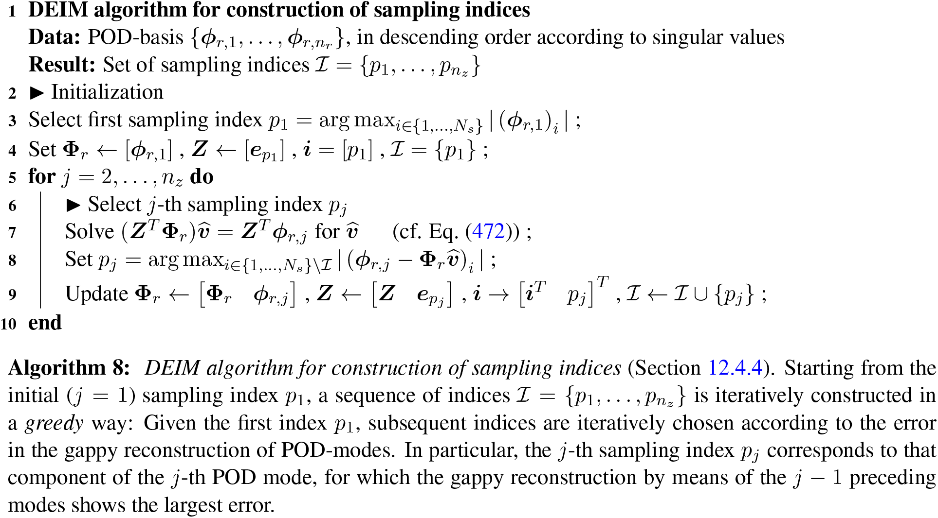
In Algorithm 9, the regularization of the cost function
In Table 8, the correspondence between the notations employed here and those in [78], p.206, is provided.
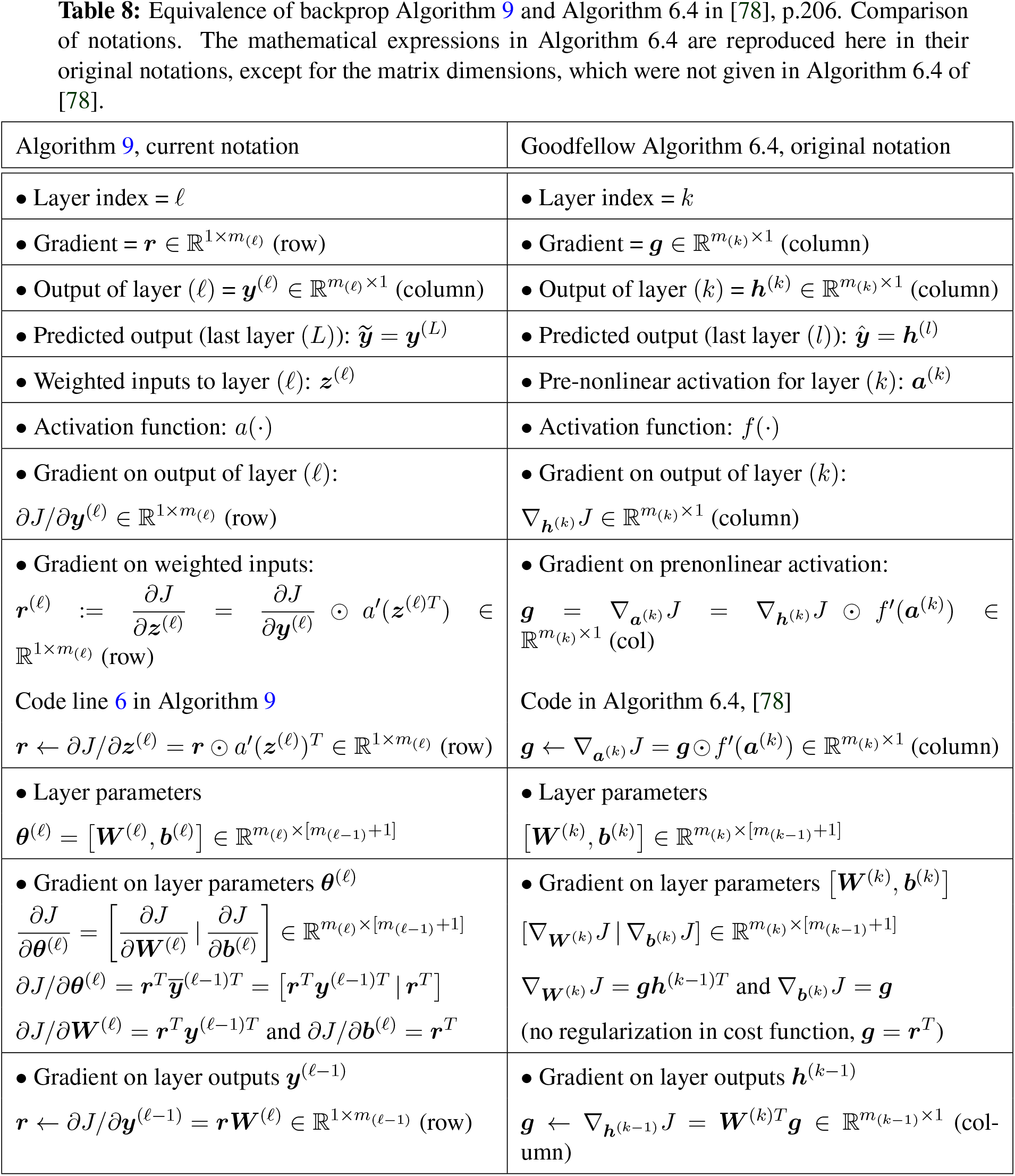
An alternative block diagram for the folded RNN with LSTM cell corresponding to Figure 81 is shown Figure 152 below:
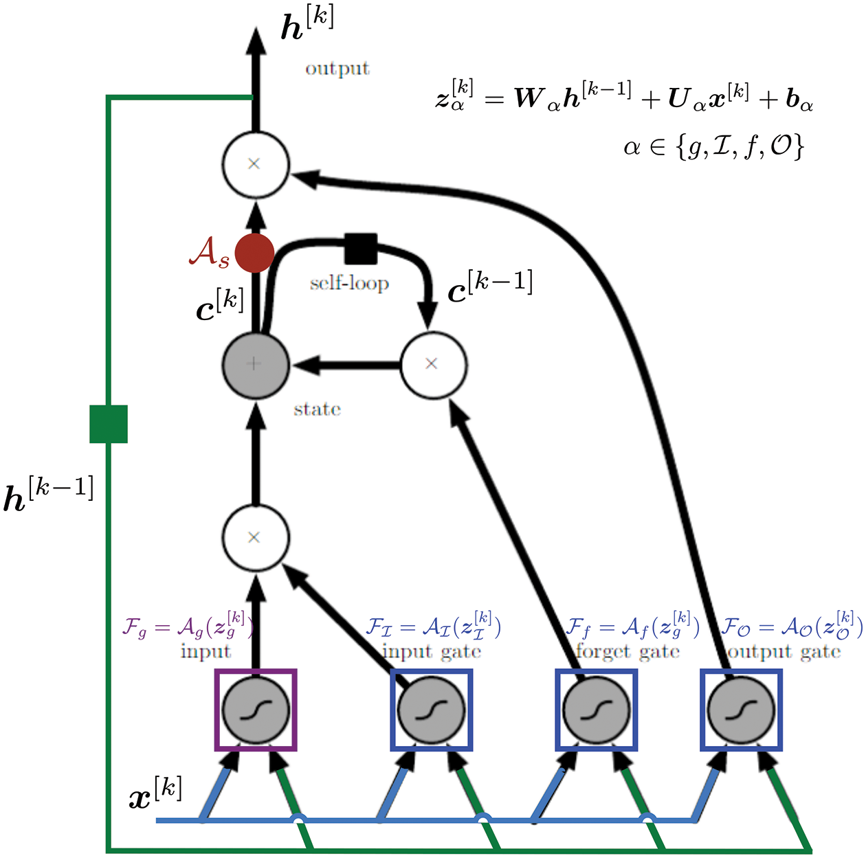
Figure 152: Folded RNN and LSTM cell, two feedback loops with delay, block diagram. Typical state
Figure 10.16 in the online book Deep Learning by Goodfellow et al. (2016), Chap.10, p.405 (referred to here as “DL-A”, or “Deep Learning, version A”), was either incomplete with missing important details. Even the updated Figure 10.16 in [78], p.398 (referred to as “DL-B”), was still incomplete (or incorrect).
The corrected arrows, added annotations, and colors correspond to those in the equivalent Figure 81. The corrections are described below.
Error 1: The cell state
Error 2: The hidden-state feedback loop (green) should start from the hidden state
Error 3: Four pairs of arrows pointing into the four gates
3 Conditional Gaussian distribution
The derivation of Eqs. (377)-(379) is provided here helps develop a better feel for the Gaussian distribution, and facilitates the understanding of the conditional Gaussian process posterior described in Section 8.3.2.
If two sets of variables have a joint Gaussian distribution, i.e., these two sets are jointly Gaussian, then the conditional probability distribution of one set given the other set is also Gaussian.339 The two sets of variables considered here is the observed values in
then expand the exponent in the Gaussian joint probability Eq. (368), with
which is also a quadratic form in terms of
where the constant is independent of
and compare to Eq. (521), then for the conditional distribution
in which Eq. (523)2 had been used.
At this point, the submatrices
the 2nd row gives rise to a system of two equations for two unknowns
in which the covariance matrix
from the first equation, and leads to
which, after using Eq. (527) to identify
Remark 3.1. Another way to obtain indirectly Eq. (379) and Eq. (378), without derivation, is to use the identity of the inverse of a partitioned matrix in Eq. (531), as done in [130], p. 87:
This method is less satisfactory since without derivation, there is no feel of where the matrix elements in Eq. (531) came from. In fact, the derivation of the 1st row of Eq. (531) follows exactly the same line as for Eqs.(528)-(530). The 2nd row in Eq. (531) looks complex, but before getting into its derivation, we note that exactly the same line of derivation for the 1st row can be straightforwardly followed to arrive at different, and simpler, expressions of the 2nd-row matrix elements
It can be easily verified that
To derive the 2nd row of Eq. (531), premultiply the 1st row (which had been derived as mentioned above) of Eq. (532) by
To make the right-hand side become
Yet another way to derive Eqs. (378)-(379) is to use the more complex proof in [248], p. 429, which was referred to in [234], p. 200 (see also Footnote 242). ■
In summary, the above derivation is simpler and more direct than in [130], p. 87, and in [248], p. 429.
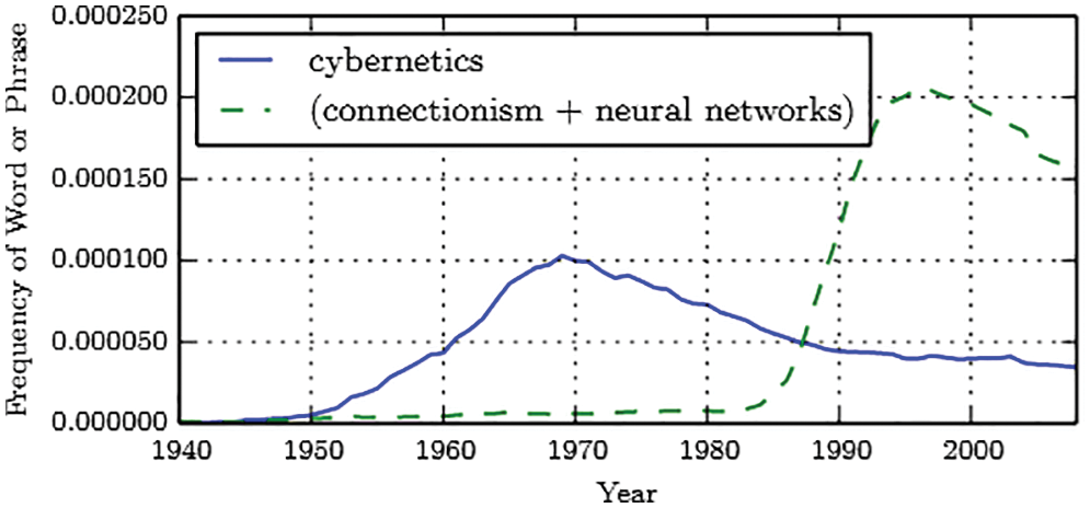
Figure 153: The first two waves of AI, according to [78], p.13, showing the “cybernetics” wave (blue line) started in the 1940s peaked before 1970, then gradually declined toward 2006 and beyond. The results were based on a search for frequency of words in Google Books. It was mentioned, incorrectly, that the work of Rosenblatt (1957-1962) [1]-[2] was limited to one neuron; see Figure 42 and Figure 133. (Figure reproduced with permission of the authors.)
4 The ups and downs of AI, cybernetics
The authors of [78], p.13, divided the wax-and-wane fate of AI into three waves, with the first wave called the “cybernetics” that started in the 1940s, peaked before 1970, then began a gradual descent toward 1986, when the second wave picked up with the publication of [22] on an application of backpropagation to psychology; see Section 13.4.1 on a history of backpropagation. Since Goodfellow (the first author of [78]) worked at Google at the time, and would have access to the scanned books in the Google Books collection to do the search. For a concise historical account of “cybernetics”, see [425].
We had to rely on Web of Science to do the “topic” search for the keyword “cyberneti*”, i.e., using the query ts=(cyberneti*), with “*” being the search wildcard, which can stand for any character that follows. Figure 154 is the result,341 spanning an astoundingly vast and diverse number of more than 100 categories,342 listed in descending order of number of papers in parentheses: Computer Science Cybernetics (2,665 papers), Computer Science Artificial Intelligence (601), Engineering Electrical Electronic (459),..., Philosophy (229),..., Social Sciences Interdisciplinary (225),..., Business (132),..., Psychology Multidisciplinary (128),..., Psychiatry (90),..., Art (66),..., Business Finance (43),..., Music (31),..., Religion (27),..., Cell biology (21),..., Law (21),...
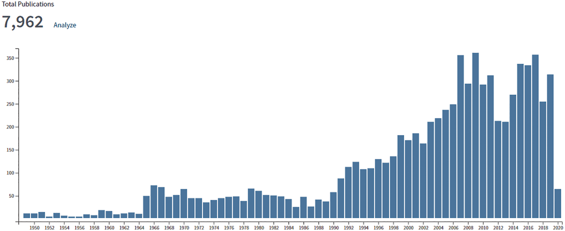
Figure 154: Cybernetics papers, (Appendix 4). Web of Science search on 2020.04.15, having more than 100 Web of Science categories. The first paper was [426]. There was no clear wave that crested before 1970, but actually the number of papers in Cybernetics continue to increase over the years.
The first paper in 1949 [426] was categorized as Mathematics. More recent papers include Biological Science, e.g., [427], Building Construction, e.g., [428], Accounting, e.g., [429].
It is interesting to note that McCulloch who co-authored the well-known paper [430] was part of the original cybernetics movement that started in the 1940s, as noted in [431]:
“Warren McCulloch, the “chronic chairman” and founder of the cybernetics conferences.343 An eccentric physiologist, McCulloch had coauthored a foundational article of cybernetics on the brain’s neural network.”
But McCulloch & Pitt’s 1943 paper [430]–often cited in artificial-neural-network papers (e.g., [23], [12]) and books (e.g., [78]), and dated six years before [426]–was placed in the Web of Science category “Biology; Mathematical & Computational Biology,” and thus did not show up in the search with keyword “cyberneti*” shown in Figure 154. A reason is [430] did not contain the word “cybernetics,” which was not invented until 1948 with the famous book by Wiener, and which was part of the title of [426]. Cybernetics was a “new science” with a “mysterious name and universal aspirations” [431], p.5.
“What exactly is (or was) cybernetics? This has been a perennial ongoing topic of debate within the American Society for Cybernetics throughout its 50-year history.... the word has a much older history reaching back to Plato, Ampère (“Cybernétique = the art of growing”), and others. “Cybernetics” comes from the Greek word for governance, kybernetike, and the related word, kybernetes, steersman or captain” [432].
Steering a ship is controlling its direction. [433] defined cybernetics as
Figure 155: Cybernetics papers, (Appendix 4). Web of Science search on 2020.04.17, ALL Computer-Science categories (3,555 papers): Cybernetics (2,666), Artificial Intelligence (602), Information Systems (432), Theory Methods (300), Interdisciplinary Applications (293), Software Engineering (163). The wave crest was in 2007, with a tiny bump in 1980.
“... (feedback) control and communication theory pertinent to the description, analysis, or construction of systems that involve (1) mechanisms (receptors) for the reception of messages or stimuli, (2) means (circuits) for communication of these to (3) a central control unit that responds by feeding back through the system (4) instructions that (will or tend to) produce specific actions on the part of (5) particular elements (effectors) of the system.... The central concept in cybernetics is a feedback mechanism that, in response to information (stimuli, messages) received through the system, feeds back to the system instructions that modify or otherwise alter the performance of the system.”
Even though [432] did not use the word “control”, the definition is similar:
“The core concepts involved natural and artificial systems organized to attain internal stability (homeostasis), to adjust internal structure and behavior in light of experience (adaptive, self-organizing systems), and to pursue autonomous goal-directed (purposeful, purposive) behavior.” [432]
and is succinctly summarized by [434]:
“If “cybernetics” means “control and communication,” what does it not mean? It would be difficult to think of any process in which nothing is either controlled or communicated.”
which is the reason why cybernetics is found in a large number of different fields. [431], p.4, offered a similar, more detailed explanation of cybernetics as encompassing all fields of knowledge:
“Wiener and Shannon defined the amount of information transmitted in communications systems with a formula mathematically equivalent to entropy (a measure of the degradation of energy). Defining information in terms of one of the pillars of physics convinced many re searchers that information theory could bridge the physical, biological, and social sciences. The allure of cybernetics rested on its promise to model mathematically the purposeful behavior of all organisms, as well as inanimate systems. Because cybernetics included information theory in its purview, its proponents thought it was more universal than Shannon’s theory, that it applied to all fields of knowledge.”
Figure 156: Cybernetics papers, (Appendix 4). Web of Science search on 2020.04.15 (two days before Figure 155), category Computer Science Cybernetics (2,665 papers). The wave crest was in 2007, with a tiny bump in 1980.
Figure 157: Cybernetics papers, (Appendix 4). Web of Science search on 2020.04.15 (two days before Figure 155), category Computer Science Artificial Intelligence (601 papers). Similar to Figure 156, the wave crest was in 2007, but with no tiny bump in 1980, since the first paper was in 1982.
In 1969, the then president of the International Association of Cybernetics asked “But after all what is cybernetics? Or rather what is it not, for paradoxically the more people talk about cybernetics the less they seem to agree on a definition,” then identified several meanings: A mathematical control theory, automation, computerization, communication theory, study of human-machine analogies, philosophy explaining the mysteries of life! [431], p.5.
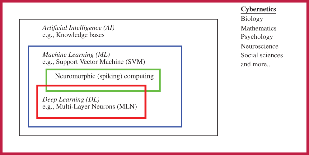
Figure 158: Artificial Intelligence (AI), Machine Learning (ML), and Deep Learning (DL). Cybernetics is broad and encompasses many fields, including AI. See also Figure 6.
So was there a first wave in AI called “cybernetics” ? Back in Oct 2018, we conveyed our search result at that time–which was similar to Figure 154, but clearly did not support the existence of the cybernetics wave shown in Figure 153–to Y. Bengio of [78], who then replied:
“Ian [Goodfellow] did those figures, but my take on your observations is that the later surge in ’new cybernetics’ does not have much more to do with artificial neural networks. I’m not sure why the Google Books search did not catch that usage, though.”
We then selected only the categories that had the words “Computer Science” in their names; there were only six such categories among more than 100 categories, as shown in Figure 155. A similar figure obtained in Oct 2018 was also shared with Bengio, who had no further comment. The wave crest in Figure 155 occurred in 2007, with a tiny bump in 1980, but not before 1970 as in Figure 153.
Figure 156 is the histogram for the largest single category Computer Science Cybernetics with 2,665 papers. In this figure, similar to Figure 155, the wave crest here also occurred in 2007, with a tiny bump in 1980.
Figure 157 is the histogram for the category Computer Science Artificial Intelligence with 601 papers. Again here, similar to Figure 155 and Figure 156, the wave crest here also occurred in 2007, with no bump in 1980. The first document, a 5-year plan report of Latvia, appeared in 1982. There is a large “impulse” of number of papers in 2007, and a smaller “impulse” in 2014, but no smooth bump. There were no papers for 9 years between 1982 and 1992, in which a single paper appeared in the series “Lecture Notes in Artificial Intelligence” on cooperative agents.
Cybernetics, including the original cybernetics moment, as described in [431], encompassed many fields and involved many researchers not working on neural nets, such as Wiener, John von Neumann, Margaret Mead (anthropologist), etc., whereas the physiologist McCulloch co-authored the first “foundational article of cybernetics on the brain’s neural network”. So it is not easy to attribute even the original cybernetic moment to research on neural nets alone. Moreover, many topics of interest to researchers at the time involve natural systems (including [430]), and thus natural intelligence, instead of artificial intelligence.
Cite This Article
 Copyright © 2023 The Author(s). Published by Tech Science Press.
This work is licensed under a Creative Commons Attribution 4.0 International License , which permits unrestricted use, distribution, and reproduction in any medium, provided the original work is properly cited.
 Downloads
 Citation Tools