
 Submit a Paper
 Propose a Special lssue
 Open Access
ARTICLE
Dynamical Analysis of the Stochastic COVID-19 Model Using Piecewise Differential Equation Technique
1
Department of Mathematics, Huzhou University, Huzhou, 313000, China
2
Department of Mathematics, Imam Mohammad Ibn Saud Islamic University, Riyadh, 12211, Saudi Arabia
3
Department of Mathematics, Government College University, Faisalabad, 38000, Pakistan
4
Department of Mathematics and Statistics, College of Science, Taif University, P.O.Box 11099, Taif, 21944, Saudi Arabia
* Corresponding Author: Saima Rashid. Email:
(This article belongs to the Special Issue: Recent Developments on Computational Biology-I)
Computer Modeling in Engineering & Sciences 2023, 137(3), 2427-2464. https://doi.org/10.32604/cmes.2023.028771
Received 06 January 2023; Accepted 20 March 2023; Issue published 03 August 2023
 View Full Text
 Download PDF
Abstract
Various data sets showing the prevalence of numerous viral diseases have demonstrated that the transmission is not truly homogeneous. Two examples are the spread of Spanish flu and COVID-19. The aim of this research is to develop a comprehensive nonlinear stochastic model having six cohorts relying on ordinary differential equations via piecewise fractional differential operators. Firstly, the strength number of the deterministic case is carried out. Then, for the stochastic model, we show that there is a critical number that can predict virus persistence
and infection eradication. Because of the peculiarity of this notion, an interesting way to ensure the existence
and uniqueness of the global positive solution characterized by the stochastic COVID-19 model is established by
creating a sequence of appropriate Lyapunov candidates. A detailed ergodic stationary distribution for the stochastic
COVID-19 model is provided. Our findings demonstrate a piecewise numerical technique to generate simulation
studies for these frameworks. The collected outcomes leave no doubt that this conception is a revolutionary
doorway that will assist mankind in good perspective nature.
that can predict virus persistence
and infection eradication. Because of the peculiarity of this notion, an interesting way to ensure the existence
and uniqueness of the global positive solution characterized by the stochastic COVID-19 model is established by
creating a sequence of appropriate Lyapunov candidates. A detailed ergodic stationary distribution for the stochastic
COVID-19 model is provided. Our findings demonstrate a piecewise numerical technique to generate simulation
studies for these frameworks. The collected outcomes leave no doubt that this conception is a revolutionary
doorway that will assist mankind in good perspective nature. Keywords
Coronavirus disease 2019 is a contagious infection transmitted by the serious acute respiratory syndrome coronavirus 2 (SARS-CoV-2). Headaches, congestion, weariness, muscle aches, breathlessness, diminished appetite, taste and aroma are typical problems. Effects including bronchitis, multi-organ failure, chronic pulmonary disruption phenomenon, septicaemia, tachycardia, cardiogenic shock, thrombosis, cardiac arrest, convulsions, meningitis, dementia and Guillain Barré syndrome may occur in certain people [1]. The implantation phase might last anywhere from two to fourteen days.
The new coronavirus transmits through fluids created by inhaling, breathing or conversing. Liquids emitted by sick individuals are breathed into the trachea of others, developing quality infestations. If individuals contact infected materials and then their faces with unhygienic fingers after the particles tumble on them, they can transmit the disease. Whereas saliva and mucous are key infection transmitters, new evidence indicates that the infection is transferred via faecal contamination pathways. Aerosol-generating methods (AGMs) potentially assist in simpler pathogen propagation than standard pathogen propagation.
SARS-CoV-2 shares characteristics with the severe acute respiratory syndrome coronavirus (SARS-CoV or SARS-CoV1), an encapsulated, newly infected cause that primarily attacks the trachea after entering the host organism and binding to angiotensin-converting-enzyme 2 (ACE2), which is highly prevalent in atelectasis type II (AT2) keratinocytes of the respiratory system [2,3]. It is classified as a congenital illness since it is spread to people via bats as biological transmitters. According to chromosomal investigation, the infection belongs to the Betacoronavirus species and includes two bat-derived viruses [4].
COVID-19 was reported on December 31, 2019, in Wuhan, China’s Hubei region, and has since proliferated globally. On January 30, 2020, the WHO labelled the epidemic a Public Health Emergency of International Concern (PHEIC), and on March 11, 2020, it designated the disease a global epidemic [4,5]. As of August 20, 2020, 217 nations and entities, such as Pakistan, had recorded 30.6 million documented infections and 890,000 fatalities. The very first COVID-19 incidence in Pakistan was detected on February 26, 2020. On September 20, 2020, the government had 306,304 documented favourable patients, 6420 fatalities, and 292,869 recovered [6].
COVID-19 has had a negative impact on the world’s economic development, basic necessities, price volatility, cultural activities and entertainment domains, religious ceremonies, recreation, film, hospitality, academia, care facilities, and democracy. Several specifics about the spread, mitigation, and therapy of this novel ailment are being investigated by mathematicians and virologists [7–9]. Numerous studies using mathematical simulations to understand infection processes and epidemic interventions have been presented [10–14]. Tang et al. [15] developed a cohort system in which the community was classified into nine ordinary differential equations. Considering evidence from scientifically verified COVID-19 occurrences in central China during the month of January, they approximated the virus’s fundamental reproductive rate. It was discovered that prevention strategies can successfully diminish the reproductive capacity. Tang et al. [16] examined a simplified form of their earlier approach, anticipating time-dependent interaction and identification outcomes. This resulted in a lower reproductive rate than had been forecasted in their prior investigation. Li et al. [17] discussed coronavirus dissemination utilizing an SEIR approach for the incidents reported in Wuhan as well as the proportion of exported infections. It is demonstrated that implementing preventive actions, including immigration prohibitions, might be critical in understanding epidemic patterns and the chances of controlling their dissemination. In [18], it seems to be other noteworthy research where the propagation speed is regarded to be a time-dependent variable. The structure is created by adding three additional compartments to the SEIR system. Other significant breakthroughs in innovative coronavirus modelling methodologies can be discovered in [19–24].
Scientists in numerous classifications and scientific disciplines have gravitated toward using fractional systems of differential equations (DEs) in the majority of their novel evidence and investigations as a consequence of the emergence of fractional derivatives [25–27]. In addition, to see this realistically, we can resort to numerical techniques of the proliferation and evolution of numerous infections and communicable conditions, which have emerged as an intriguing issue for scholars in past centuries, employing fractional frameworks of initial value problems. While reviewing the articles, we discovered that various scholars have proposed kernels that can be employed to create fractional differential formulations. The major motivation behind this is that serious challenges exhibit signs of mechanisms that are similar to the behaviours of precise scientific expressions. Fractional calculus incorporating a power law kernel is led by the contributions of Riemann, Liouville, Cauchy, and Abel. Caputo later improved their approach, and this form has been employed in several scientific disciplines owing to its capacity to enable classical initial conditions (ICs) [28]. Prabhakar proposed an appropriate kernel containing three components as a combo of index-law and the generalized Mittag-Leffler (GML) kernel [29–31]. This form has likewise piqued the interest of numerous scholars and investigations into both concepts and implementations have been conducted [32,33].
Furthermore, the various kernels have distinctive features; for instance, index-kernel only aids in the replication of systems that indicate index-kernel tendencies. GML, the combination of the index kernel and the generalized three distinct, has its own applicability domain [34]. Because the phenomenon is multifaceted, Caputo and Fabrizio developed a novel kernel, a particular exponential kernel exhibiting Delta Dirac characteristics. A differential formulation that is becoming increasingly popular because of its capacity to repeat processes after fading memory [35–38]. Furthermore, the notion of fractional derivative having a nonsingular kernel was pioneered by this kernel, marking the inauguration of a revolutionary era in fractional calculus [39]. A scientist’s observation regarding the kernel’s non-fractionality resulted in the creation of a novel kernel, the GML function, including one component. Atangana et al. [40] proposed this formulation, which represents another advancement in the discipline of fractional calculus. The formulations have been employed successfully in a variety of fields of study. Glancing at reality and its intricacies, it is clear that these proposed kernels are insufficient to forecast all of our universe’s complicated characteristics. Following the remark, one will look for a different kernel or modified kernel, or a set of procedures that will be used to add novel differential formulations. Sabatier has proposed various kernel variants that will additionally lead to novel avenues of inquiry [41]. In addition to these remarkable breakthroughs, numerous additional notions were proposed, such as the conception of short memory and the definition of a fractional derivative in the Caputo interpretation for distinct characteristics of fractional orders. Notwithstanding the well-known formulation, which takes a fractional order to be time-dependent, the goal is to achieve a different form of variable order derivative. Wu et al. [42] proposed and implemented this scenario in chaotic theory. However, researchers have discovered that some real-world phenomena demonstrate mechanisms exhibiting varying behaviours as a factor of space and time. A transition from deterministic to stochastic, either from index-law to exponential decay, is an example. Because conventional differential formulations may be incapable of accounting for these tendencies, piecewise differential/integral formulations were devised to cope with issues manifesting crossover phenomena [43]. The primary goal of this article is to present a detailed evaluation, potential implementations, strengths and shortcomings of these two notions.
Mathematical modelling is a critical technique for understanding the transmission of a contagious illness, making predictions, and developing prevention and extinction tactics. Inspired by the aforesaid research, we propose to construct a stochastic framework to examine the impact of quarantine and isolation in reducing the transmission of the coronavirus epidemic in Pakistan via the piecewise differential operators. Pakistan is an emerging nation in the midst of an economic, environmental, and strategic crisis. The region’s health sector is indeed inefficient and faces several issues. Atangana et al. [44] recently proposed the notions of piecewise differential/integral formulations. This revolutionary notion may represent the direction of modelling, as we propose in this work a progressive frontier to analyze epidemiological challenges involving crossover behaviours. A COVID-19 model in Pakistan will be discussed in this presentation stochastically. We will presume that real world propagation reveals waves exhibiting diverse chaotic structures, classical, local/nonlocal, randomness and that a permutation depending on the aforementioned mechanisms can lead to various tendencies. Furthermore, the qualitative characteristics of the aforesaid model are displayed in terms of Brownian motion, such as the existence-uniqueness of the global positive solutions, ergodic stationary distribution, extinction and persistence of the epidemic.
The remainder of the article is organized as follows. Section 2 discusses the preliminaries, framework construction, which is constructed on a variety of assumptions. Then we analyze the strength number of the deterministic COVID-19 model. Section 3 investigates the existence-uniqueness of the global non-negative solution of a stochastic system and calculates the crucial parameter that can readily decide the extermination and permanence of the infection. We additionally show that an ergodic stationary distribution emerges in the stochastic COVID-19 model. Section 4 introduces several simulation studies to illustrate the conceptual framework and illustrate the impacts of environmental white noise. Section 5 describes the results and discussion related to numerical findings. To conclude this work, several findings and appendices are offered.
Taking into account the underlying hypotheses (Fig. 1), we construct a quantitative framework to investigate the behaviors of six classifications of people: susceptible
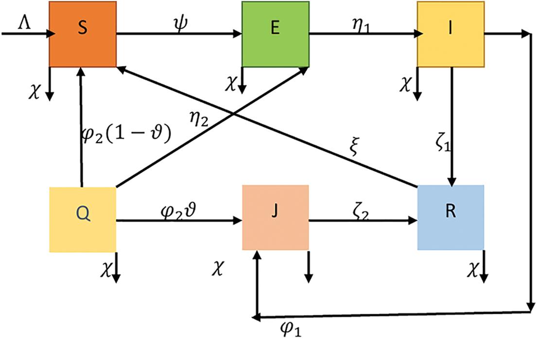
Figure 1: Schematic diagram of COVID-19 epidemic model
The vulnerable group expands by
The vulnerable people who have not yet manifested pathological changes but are susceptible to infection have increased the proportion of people in the
People in the contaminated group acquire COVID-19 indications, resulting in an estimated prevalence. It diminishes at a rate of
The associated dynamic scheme of ordinary DEs COVID-19 propagation mechanism was proposed by [45] as follows:
supplemented to the positive ICs
Furthermore, current outcomes indicate that white noise can disrupt the transmission of contagious diseases, population movement, and the formulation of prevention mechanisms. As a result, an increasing number of researchers have researched the appropriate stochastic models (see [46–48]). In [49], Atangana et al. presented deterministic-stochastic modelling with crossover effects. Rashid et al. [50] proposed the novel dynamics of a stochastic fractal-fractional immune effector response to viral infection via latently infectious tissues. Regarding the epidemiologist’s ideas, we assume that randomized white noise is independent and directly proportional to six cohorts. The stochastic form pertaining to scheme (1) can therefore be represented by the stochastic differential equations shown below:
where
where
The formulation of the Atangana-Baleanu derivative is represented below:
where
3 Qualitative Aspects of COVID-19 Model
In this section, we will discuss some qualitative aspects of the deterministic and stochastic characteristics of the COVID-19 models (1) and (2), respectively.
For COVID-19 model (1), there are two kind of steady states. The first one is disease-free equilibrium point (DFEP)
Notice that if
where
Theorem 3.1. (i)If
(ii)If
Proof. The proof can be followed by [45].
In previous decades, the idea of reproduction has been extensively used in epidemiological modelling since it has been recognized as a valuable mathematical tool for evaluating reproduction in a specific illness. According to the concept proposed by Atangana [52], one will identify two components
will be analyzed to generate reproductive number [53]. The component
and
At disease free equilibrium
Therefore, we have
Then,
gives
Also,
3.3 Dynamic of the Stochastic COVID-19 Model
In this paper, suppose a complete probability space
Next, we will examine at the d-dimensional stochastic DE
subject to intial condition
Now
where
3.4 Existence-Uniqueness of the Global Non-Negative Solution
Theorem 3.2. Suppose there is a unique solution
Proof. Our argument is predicated on the research of Mao et al. [55]. Because the parameters of scheme (2) are Lipschitz continuous locally. As a result, there is a unique local solution
Setting
Introducing a
The positivity of the
implementing Ito’s rule, we can obtain that
where
Therefore, we derive
Furthermore, we have
Implementing expectation gives
For
where
Thus, we find
3.5 Basic Reproduction Number for Stochastic Model
Utilizing fourth compartment of the model (2), we have
Considering Ito’s formulation for a twice differentiable mapping
where
The next generation matrices are
3.6 Extinction and Persistence of the Disease
One of the primary challenges in epidemiological data is how to control infection behaviours so that the infection becomes endangered and persists throughout time. In this part, we attempt to determine the important threshold for pathogen extermination and permanence.
Lemma 3.1. For the initial settings
then
Also, if
Theorem 3.3. Suppose that
(i) If
which means the diseases will be eliminated from a community.
(ii) If
which means the diseases will persist in the community.
Proof. Implementing the Ito’s formula to
Integrating the aforesaid equation from
By the strong law of large numbers for martingales [56], we have
According to the superior limit and considering stochastic comparison theorem, we have
Thus,
As a result, the infection will be exterminated in the community.
(ii) Introducing
Utilizing the fact of
Then,
Assume that
Integrating both sides of (19), we find
where
Utilizing Lemma 3.1, we find from (20)
Thus, if
3.7 Ergodic Stationary Distribution (ESD)
In this subsection, we will discuss several perspectives about the stationary distribution. Despite the fact that there is no EEP of the stochastic process (2), we wish to find the existence of an ESD, which demonstrates the virus’s endurance. Several noteworthy Has’Minskii theory outcomes can be referenced in [57].
Lemma 3.2. ([58]) The Markov technique
(i) A positive number
(ii) there exists a positive
for all
We shall establish assumptions that assure the formation of an ESD relying on Has’minskii’s hypothesis [57].
Theorem 3.4. Suppose that
Proof. Theorem 3.2 proof must meet the criteria of Lemma 3.2. Ensure that (i) satisfies. The associated diffusion matrix of framework (2) appears to be represented by
Because the matrix
where
where
Implementing the generalized Ito’s technique [51] to
Suppose
Then, it follows that
Analogously, we have
where
Also, we have
Utilizing (21)–(24), we then find that
We describe it for simplicity as
and
We can now design a bounded compact region
where
and
For simplicity, we can subdivide
Evidently,
Case I. For each
Case II. For each
Case III. For each
Case IV. For each
Case V. For each
Case VI. For each
Case VII. For each
Case VIII. For each
Case IX. For each
Case X. For each
As a result of (26)–(39), we have
This demonstrates that requirement (ii) is satisfied. As a result of the verification of the requirements in Lemma 3.2, the evidence is fulfilled.
4 Numerical Procedures of COVID-19 Framework for Various Fractional Derivative Operators
4.1 Caputo Fractional Derivative Operator
In this part, we will investigate the dynamical behaviour of COVID-19 transmission, which displays three patterns for a country, involving classical, index-law, and eventually stochastic processes. In this scenario, if we define
Here, we apply the technique described in [44] for the scenario of Caputo’s derivative to analyze quantitatively the piecewise structure (41)–(43). We commence the technique as follows:
It follows that
where
and
4.2 Caputo-Fabrizio Fractional Derivative Operator
In this section, we will examine the system dynamics of COVID-19 propagation, which shows three phases for a particular country, comprising classical, exponential decay law, and finally stochastic mechanisms. If we describe
Here, we apply the technique described in [44] for the scenario of Caputo-Fabrizio derivative to analyze quantitatively the piecewise structure (47)–(49). We commence the technique as follows:
It follows that
4.3 Atangana-Baleanu Fractional Derivative Operator
Here, we will concentrate on the dynamic behavior of COVID-19 spreading in this portion, which demonstrates three main phases for a certain region, including classical, generalized Mittag-Leffler law, and lastly, stochastic causes. If we define
Here, we apply the technique described in [44] for the scenario of Atanagan-Baleanu-Caputo derivative to analyze quantitatively the piecewise structure (52)–(54). We commence the technique as follows:
It follows that
where
In this section, we will first discuss the numerical approach for the fractional model in the context of the piecewise derivatives, which is provided in [44].
As of now, the COVID-19 coronavirus infection remains among the world’s deadliest and most dangerous. There is currently no therapeutic option. In addition, because of the virus’s aggressive propagation and the presence of numerous unpredictable components (people’s interests, mammal activities, transportation, etc.), it includes a significant amount of unpredictability. We constructed a simulation for the new 2019 coronavirus infection using stochastic concepts, and we explored the disease’s propagation features and comprehended its emergence and spread in the context of community and environmental transformation via the piecewise fractional derivative operators (e.g., Caputo, Caputo-Fabrizio and Atangana-Baleanu-Caputo context). Following the implementation of the numerical approach, we will examine the physical characteristics listed in Table 1 using fractional-order

The numerical scheme for the Caputo fractional direction indicated by (41)–(43) is studied, and the findings are schematically represented in Figs. 2–4 with lowest random intensities. Furthermore, on 7 October 2021, we might use the corresponding accurate statistics
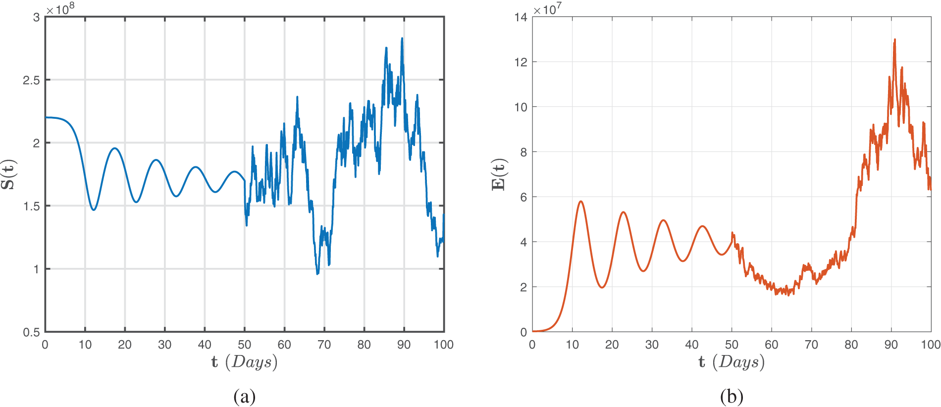
Figure 2: Numerical representations for the model (41)–(43) for the susceptible
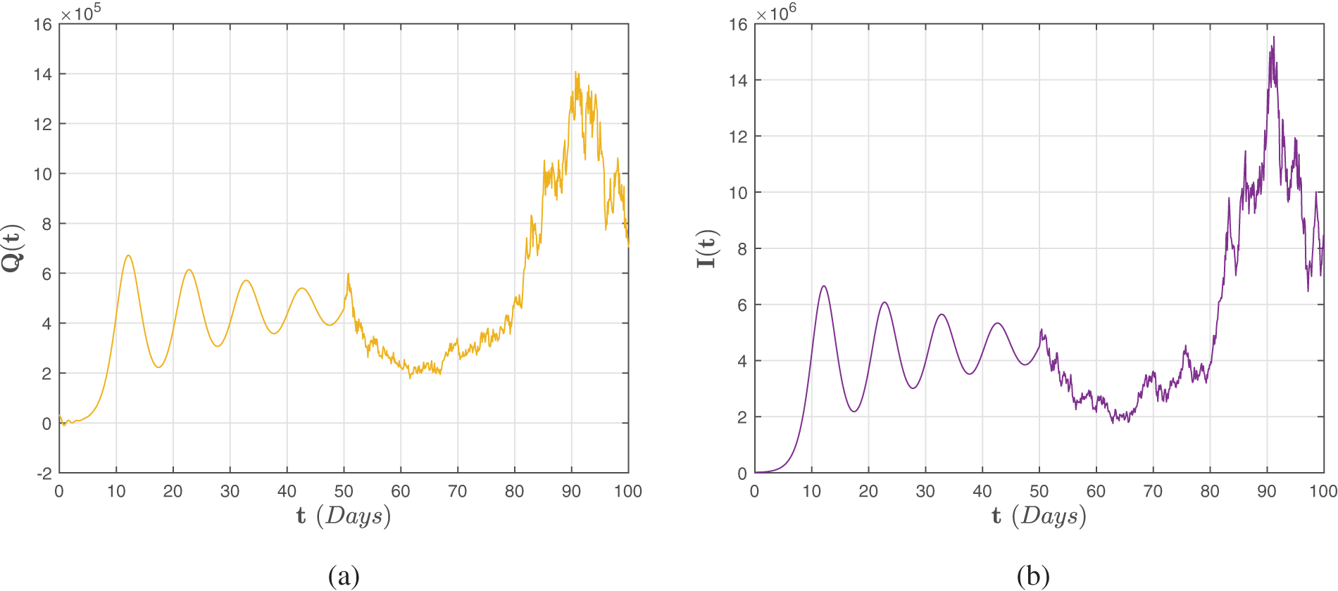
Figure 3: Numerical representations for the model (41)–(43) for the quarantined
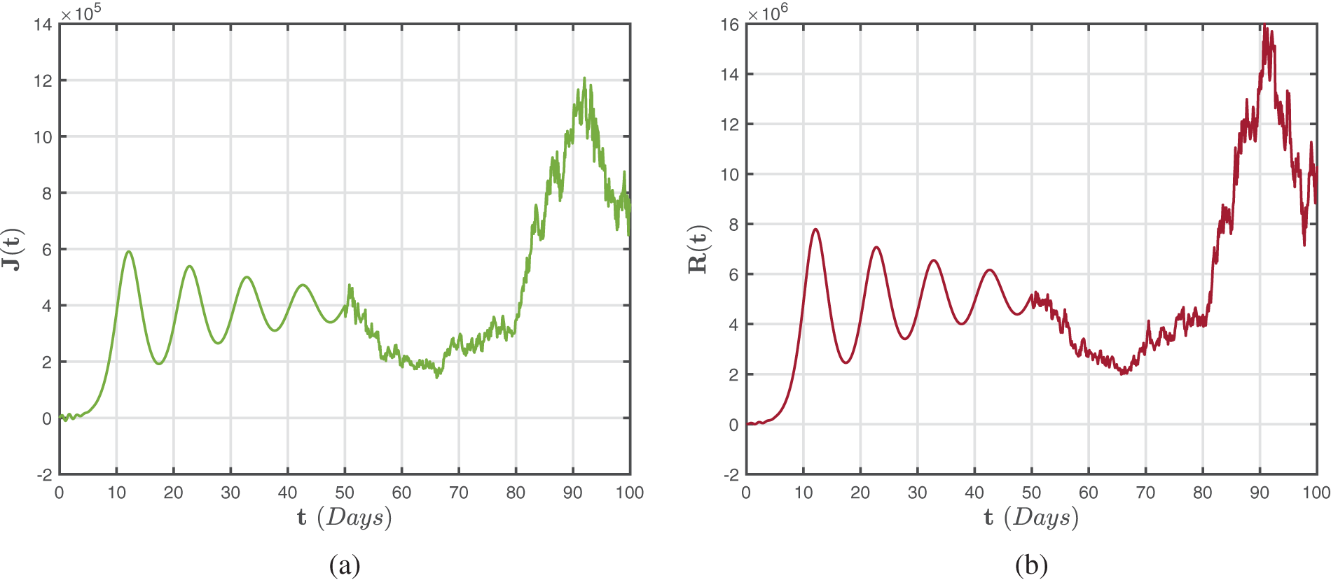
Figure 4: Numerical representations for the model (41)–(43) for the isolated
Figs. 5–7 illustrates numerical findings for the Caputo-Fabrizio sense for (47)–(49) by utilizing environmental noise values. Furthermore, the performance parameters state the biological suitability of the finding. Following that, we shall concentrate on the stochastic simulation analysis (47)–(49). Figs. 5–7 depicts the trajectories of
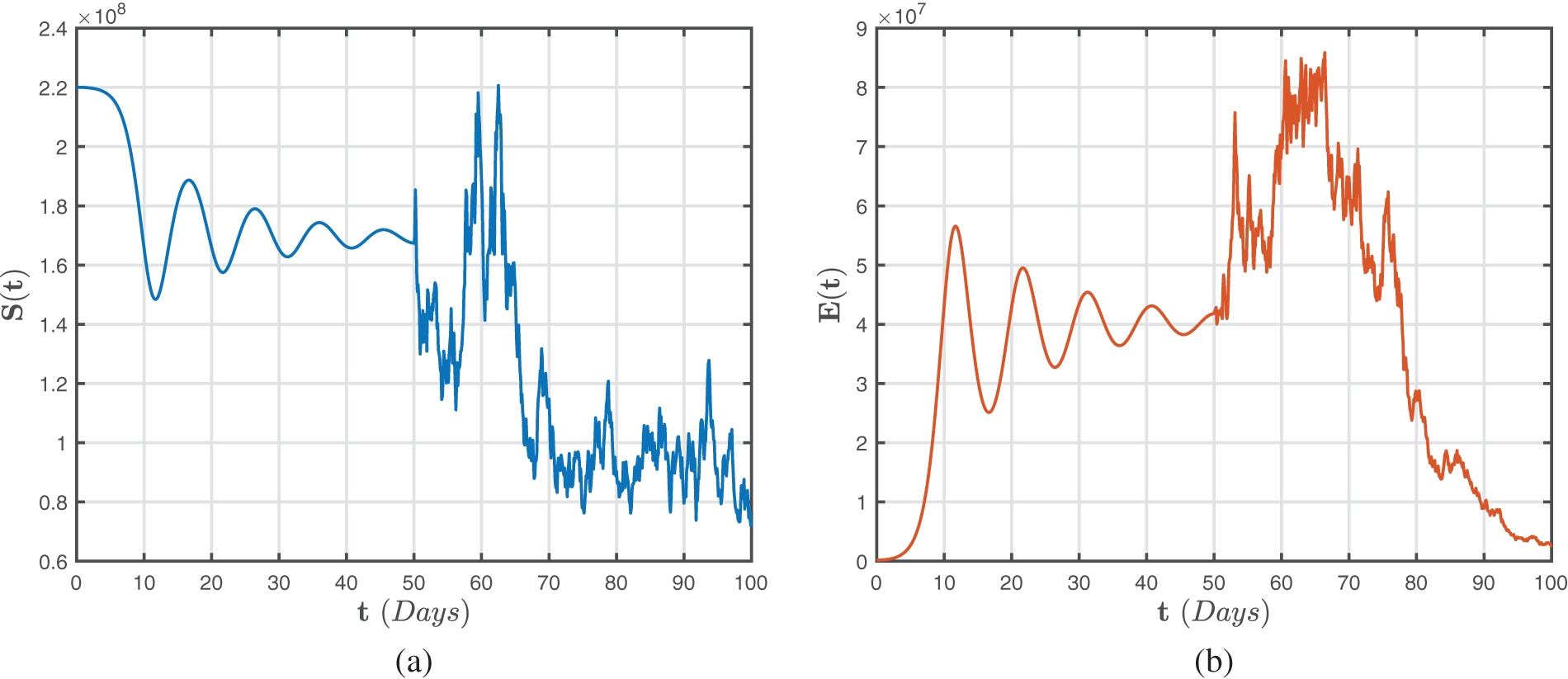
Figure 5: Numerical representations for the model (47)–(49) for the susceptible
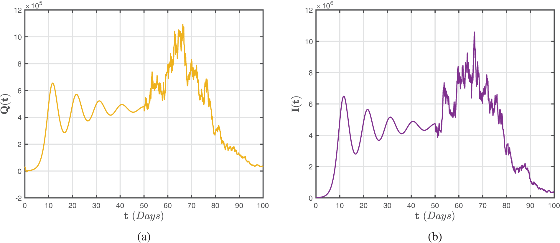
Figure 6: Numerical representations for the model (47)–(49) for the quarantined
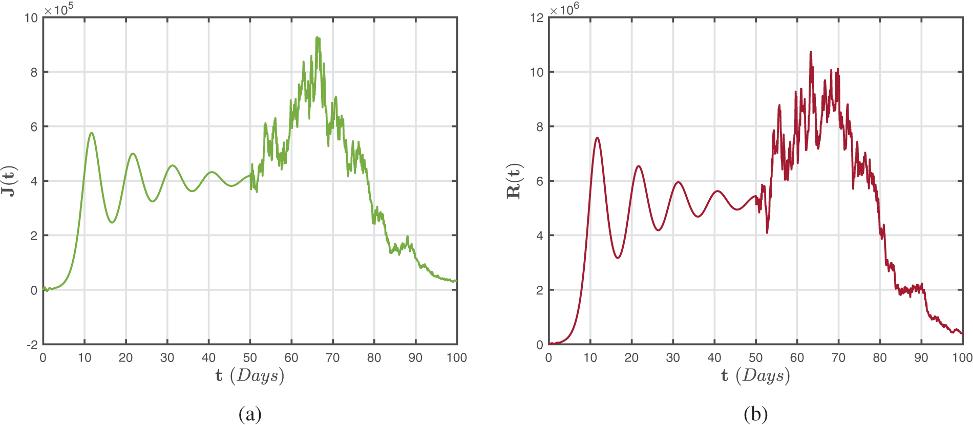
Figure 7: Numerical representations for the model (47)–(49) for the isolated
Analogously, Figs. 8–10 illustrate numerical findings for the Atangana-Baleanu-Caputo sense for (52)–(54) by utilizing environmental noise values. In particular, it may be stated that increased noise
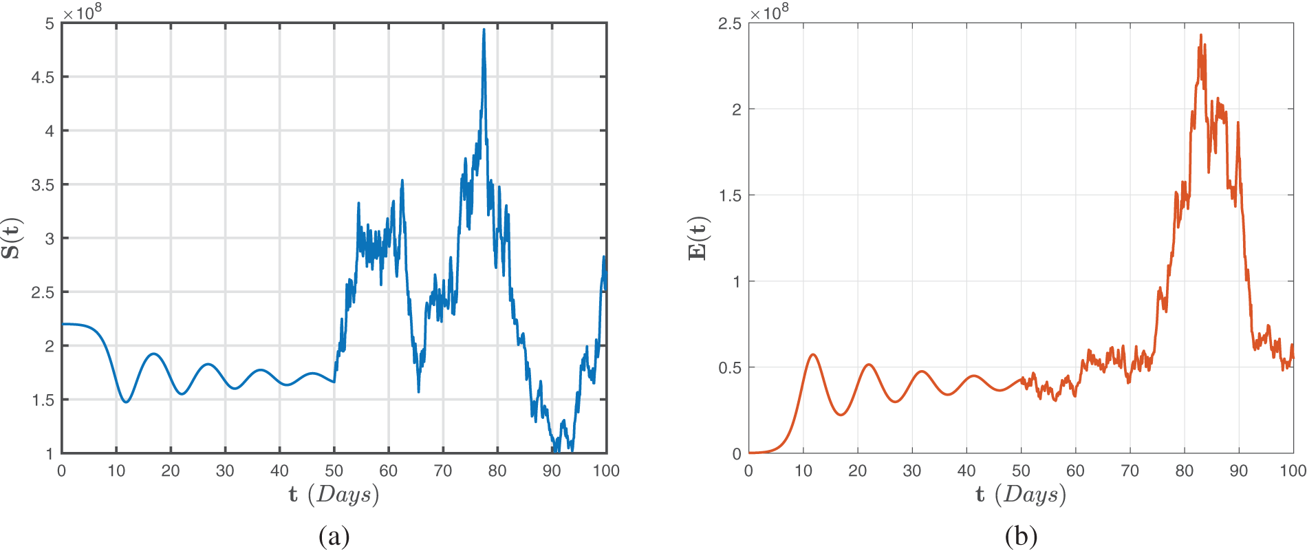
Figure 8: Numerical representations for the model (52)–(54) for the susceptible
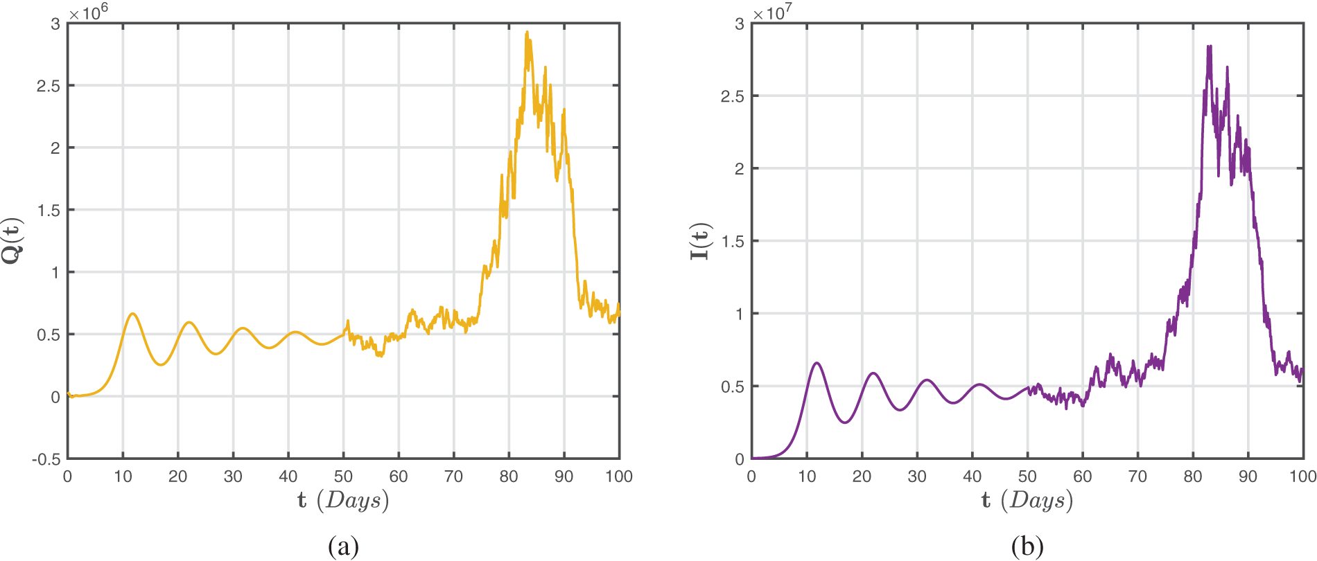
Figure 9: Numerical representations for the model (52)–(54) for the quarantined
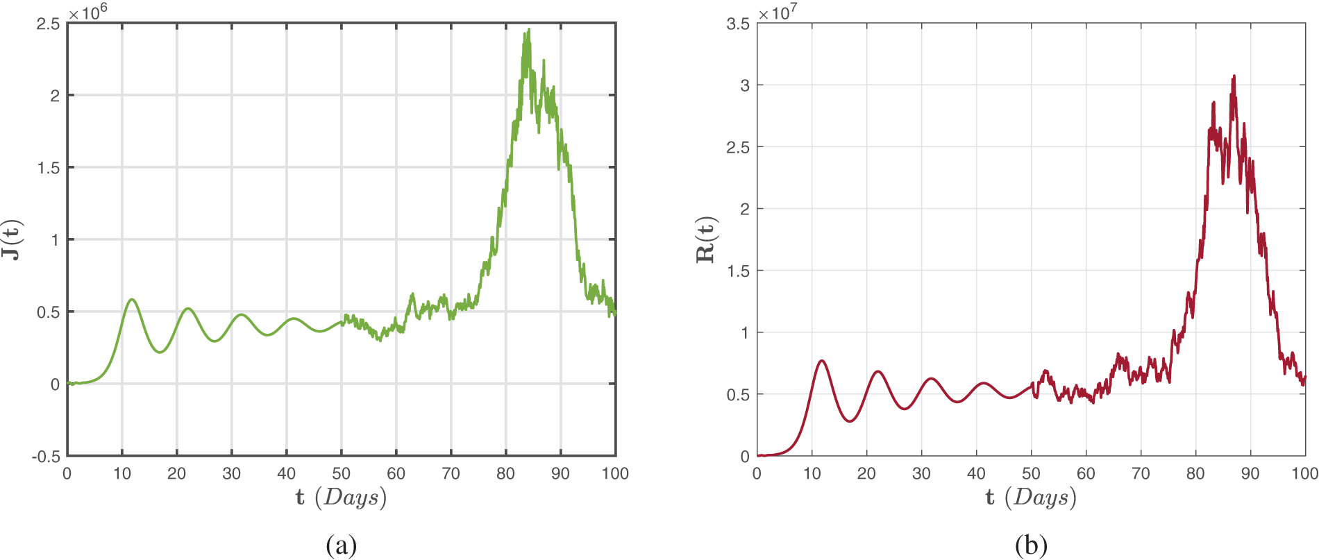
Figure 10: Numerical representations for the model (52)–(54) for the isolated
Figs. 11–13 show the chaotic behaviour of the model (52)–(54) with varying random intensities and fixed fractional-order
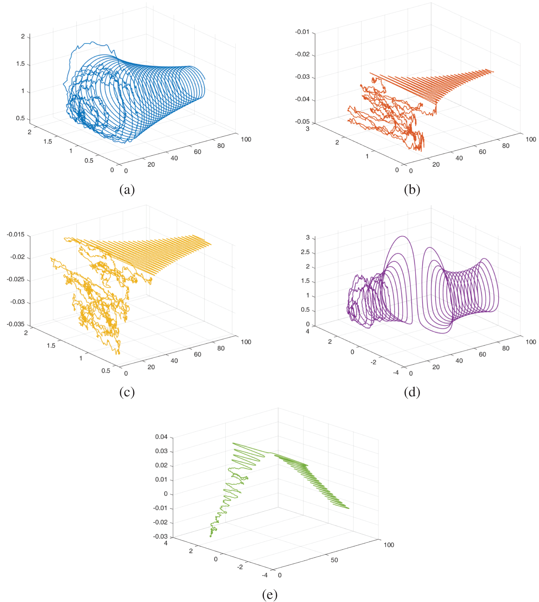
Figure 11: The dynamical behaviour of the model (52)–(54) for various cohorts when random densities
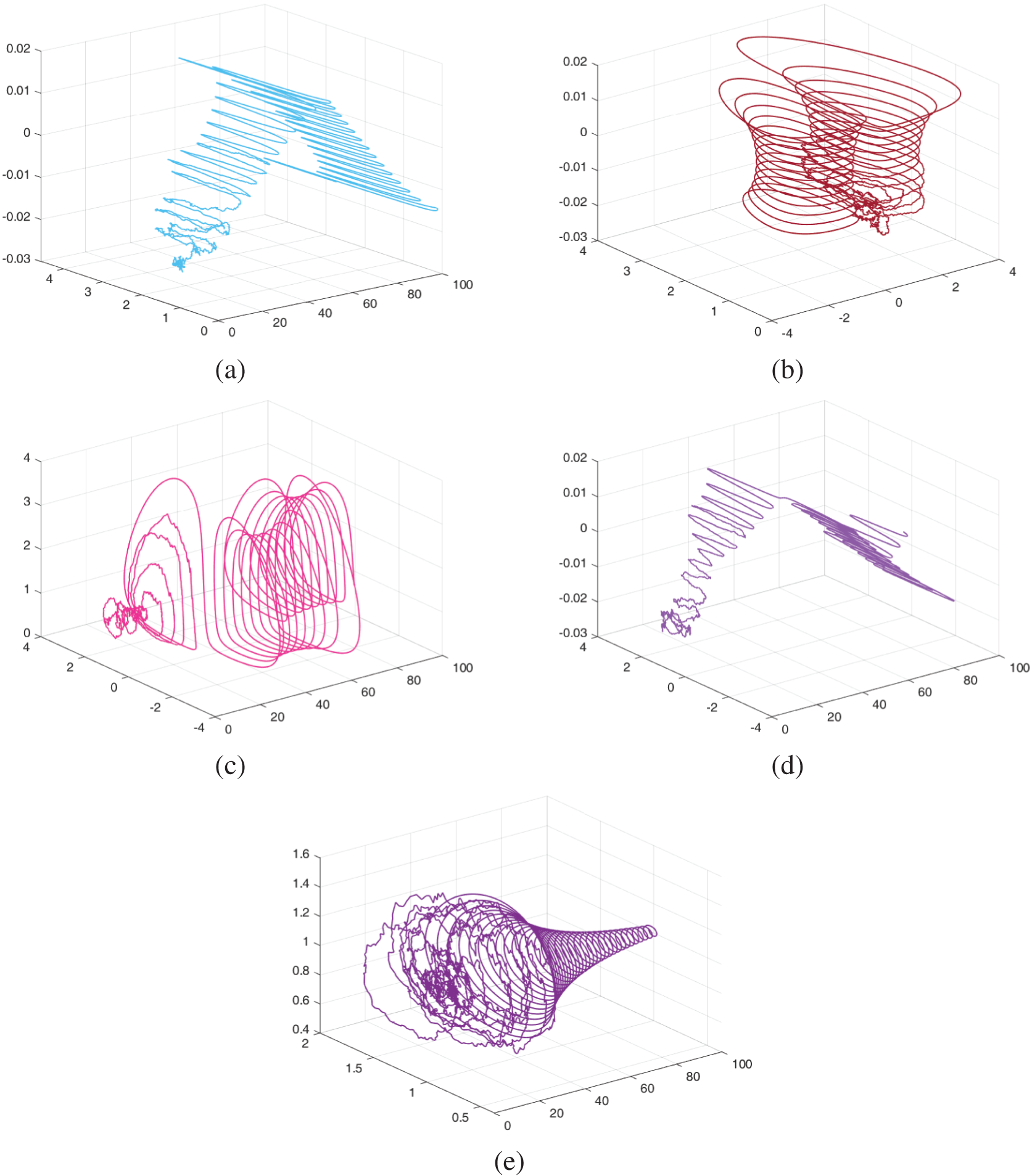
Figure 12: The dynamical behaviour of the model (52)–(54) for various cohorts when random densities
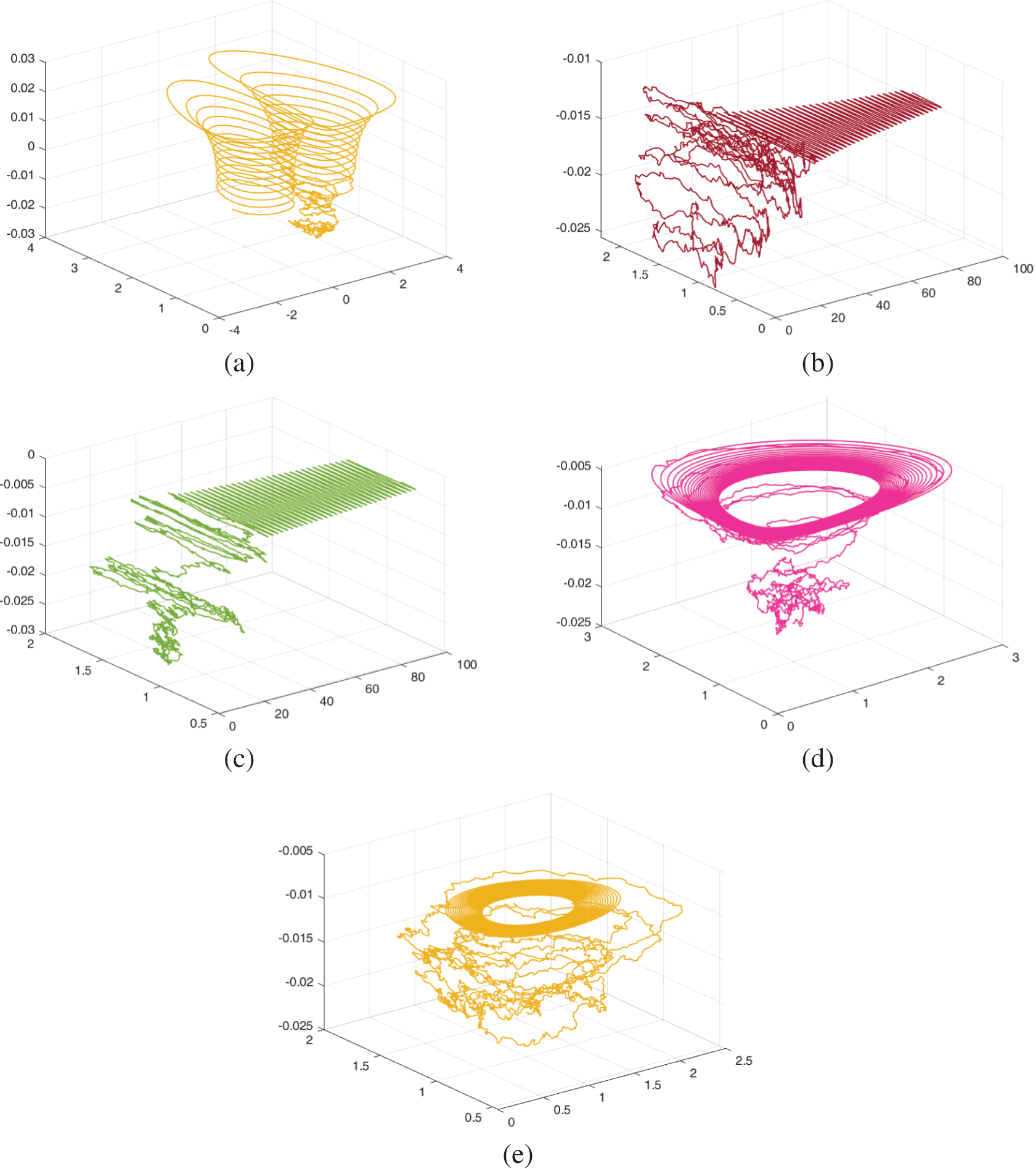
Figure 13: The dynamical behaviour of the model (52)–(54) for various cohorts when random densities
Contemporary research proposes a comprehensive framework for the existing coronavirus epidemic, including a particular emphasis on the interactions of quarantined, infected, and isolated groups via crossover behaviours. For the deterministic system, we establish the strength number. In the associated stochastic process, we first determine the extinction and permanence thresholds, followed by the ergodic stationary distribution. Even though considerable and extremely interesting outcomes have been proposed, when glancing at the transmission of COVID-19, particularly documentation from a country, someone could immediately discover that several of them exemplify crossover behaviours, such as a transition from configurations to deterministic functionalities to structures to stochastic capabilities. Employing the approach of piecewise modelling, we aimed to offer a novel aperture for modelling analogous issues. We include several illustrations to demonstrate our point. The concordance between the piecewise estimates and experimental evidence demonstrates without a dispute that this technique will aid humans in accurately predicting crossover behaviours in evolutionary biology.
Acknowledgement: The researchers would like to acknowledge Deanship of Scientific Research, Taif University for funding this work.
Funding Statement: The authors received no specific funding for this study.
Conflicts of Interest: The authors declare that they have no conflicts of interest to report regarding the present study.
References
1. World Health Organization (2020). Who.int/csr/don/12-january-2020-novelcoronavirus-china [Google Scholar]
2. Kouidere, A., Youssoufi, L. E., Ferjouchia, H., Balatif, O., Rachik, M. (2021). Optimal control of mathematical modeling of the spread of the COVID-19 pandemic with highlighting the negative impact of quarantine on diabetics people with cost-effectiveness. Chaos, Solitons and Fractals, 145(3), 110777 [Google Scholar] [PubMed]
3. Das, M., Samanta, G. (2021). Stability analysis of a fractional ordered COVID-19 model. Computational and Mathematical Biophysics, 9(1), 22–45. [Google Scholar]
4. Pacurar, C. M., Necula, B. R. (2020). An analysis of COVID-19 spread based on fractal interpolation and fractal dimension. Chaos, Solitons and Fractals, 139(3), 8. [Google Scholar]
5. Zhang, Z. (2020). Corrigendum to a novel COVID-19 mathematical model with fractional derivatives: Singular and nonsingular kernels. Chaos, Solitons and Fractals, 139(2), 110128. [Google Scholar]
6. Begum, R., Tunc, O., Khan, H., Gulzar, H., Khan, A. (2021). A fractional order Zika virus model with Mittag-Leffler kernel. Chaos, Solitons and Fractals, 146(2), 11. [Google Scholar]
7. He, Z. Y., Abbes, A., Jahanshahi, H., Alotaibi, N. D., Wang, Y. (2022). Fractional-order discrete-time SIR epidemic model with vaccination: Chaos and complexity. Mathematics, 10(2), 165. https://doi.org/10.3390/math10020165 [Google Scholar] [CrossRef]
8. Jin, F., Qian, Z. S., Chu, Y. M., Rahman, M. (2022). On nonlinear evolution model for drinking behavior under Caputo-Fabrizio derivative. Journal of Applied Analysis & Computation, 12(2), 790–806. [Google Scholar]
9. Wang, F. Z., Khan, M. N., Ahmad, I., Ahmad, H., Abu-Zinadah, H. et al. (2022). Numerical solution of traveling waves in chemical kinetics: Time-fractional Fishers equations. Fractals, 30(2), 22400051. https://doi.org/10.1142/S0218348X22400515 [Google Scholar] [CrossRef]
10. Dehingia, K., Yao, S. W., Sadri, K., Das, A., Kumar, H. S. et al. (2022). A study on cancer-obesity-treatment model with quadratic optimal control approach for better outcomes. Results in Physics, 42(1), 105963. [Google Scholar]
11. Partohaghighi, M., Veeresha, P., Akgül, A., Inc, M., Riaz, M. B. (2022). Fractional study of a novel hyper-chaotic model involving single non-linearity. Results in Physics, 42(1), 105965. [Google Scholar]
12. Zafar, Z. A., Hussain, M. T., Inc, M., Baleanu, D., Almohsenh, B. et al. (2022). Fractional-order dynamics of human papillomavirus. Results in Physics, 34(3), 105281. [Google Scholar]
13. Acay, B., Inc, M., Mustapha, U. T., Yusuf, A. (2021). Fractional dynamics and analysis for a lana fever infectious ailment with Caputo operator. Chaos, Soliton and Fractals, 153(3), 111605. [Google Scholar]
14. Rihan, F. A., Alsakaji, H. J. (2021). Dynamics of a stochastic delay differential model for COVID-19 infection with asymptomatic infected and interacting peoples: A case study in the UAE. Results in Physics, 28(5), 104658. https://doi.org/10.1016/j.rinp.2021.104658 [Google Scholar] [PubMed] [CrossRef]
15. Tang, B., Wang, X., Li, Q., Bragazzi, N. L., Tang, S. et al. (2020). Estimation of the transmission risk of the 2019-nCoVand its implication for public health interventions. Journal of Clinical Medicine, 9(2), 462–474. https://doi.org/10.3390/jcm9020462 [Google Scholar] [PubMed] [CrossRef]
16. Tang, B., Bragazzi, N. L., Li, Q., Tang, S., Xiao, Y. et al. (2020). An updated estimation of the risk of transmission of the novel coronavirus (2019-nCoV). Infectious Diseases Modelling, 5(7), 248–255. https://doi.org/10.1016/j.idm.2020.02.001 [Google Scholar] [PubMed] [CrossRef]
17. Li, Y., Wang, B., Peng, R., Zhou, C., Zhan, Y. et al. (2020). Mathematical modeling and epidemic prediction of COVID-19 and its significance to epidemic prevention and control measures. Journal of Current Scientific Research, 1(1), 19–36. [Google Scholar]
18. Qianying, L., Zhao, S., Gao, D., Lou, Y., Yang, S. et al. (2020). A conceptual model for the coronavirus disease 2019 (COVID-19) outbreak in Wuhan, China with individual reaction and governmental action. International Journal of Infectious Diseases, 93(1766), 211–216. https://doi.org/10.1016/j.ijid.2020.02.058 [Google Scholar] [PubMed] [CrossRef]
19. Khan, M. A., Atangana, A. (2020). Modeling the dynamics of novel coronavirus (2019-nCoV) with fractional derivative. Alexandria Engineering Journal, 59(4), 2379–2389. [Google Scholar]
20. Ivorra, B., Ferrández, M. R., Vela-Pérez, M., Ramos, A. M. (2020). Mathematical modeling of the spread of the coronavirus disease 2019 (COVID-19) considering its particular characteristics. The case of China. Communications in Nonlinear Science and Numerical Simulation, 88(1), 105303. https://doi.org/10.1016/j.cnsns.2020.105303 [Google Scholar] [PubMed] [CrossRef]
21. Alsakaji, H. J., Rihan, F. A., Hashish, A. (2022). Dynamics of a stochastic epidemic model with vaccination and multiple time-delays for COVID-19 in the UAE. Complexity, 2022, 1–15. [Google Scholar]
22. Zhao, T. H., Castillo, O., Jahanshahi, H., Yusuf, A., Alassafi, M. O. et al. (2021). A fuzzy-based strategy to suppress the novel coronavirus (2019-nCoV) massive outbreak. Applied and Computational Mathematics, 20, 160–176. [Google Scholar]
23. Baba, I. A., Rihan, F. A. (2022). A fractional-order model with different strains of COVID-19. Physica A, 603, 127813 [Google Scholar] [PubMed]
24. Fadaei, Y., Rihan, F. A., Rajivganthi, C. (2022). Immunokinetic model for COVID-19 patients. Complexity, 2022(1), 8321848. https://doi.org/10.1155/2022/8321848 [Google Scholar] [CrossRef]
25. Nazeer, M., Hussain, F., Ijaz, K. M., Rehman, A., El-Zahar, E. R. et al. (2021). Theoretical study of MHD electro-osmotically flow of third-grade fluid in micro channel. Applied and Computational Mathematics, 420(2), 126868. https://doi.org/10.1016/j.amc.2021.126868 [Google Scholar] [CrossRef]
26. Chu, Y. M., Shankaralingappa, B. M., Gireesha, B. J., Alzahrani, F., Khan, M. I. et al. (2021). Combined impact of Cattaneo-Christov double diffusion and radiative heat flux on bio-convective flow of Maxwell liquid configured by a stretched nano-material surface. Applied and Computational Mathematics, 419(1), 126883. https://doi.org/10.1016/j.amc.2021.126883 [Google Scholar] [CrossRef]
27. Zhao, T. H., Khan, M. I., Chu, Y. M. (2021). Artificial neural networking (ANN) analysis for heat and entropy generation in flow of non-Newtonian fluid between two rotating disks. Mathematical Methods in Applied Sciences, 46(3), 3012–3030. https://doi.org/10.1002/mma.7310 [Google Scholar] [CrossRef]
28. Caputo, M. (1967). Linear model of dissipation whose Q is almost frequency independent II. Geophysical Journal International, 13(5), 529–539. [Google Scholar]
29. Rashid, S., Abouelmagd, E. I., Sultana, S., Chu, Y. M. (2022). New developments in weighted n-fold type inequalities via discrete generalized ĥ-proportional fractional operators. Fractals, 30(2), 2240056. https://doi.org/10.1142/S0218348X22400564 [Google Scholar] [CrossRef]
30. Rashid, S., Sultana, S., Karaca, Y., Khalid, A., Chu, Y. M. (2022). Some further extensions considering discrete proportional fractional operators. Fractals, 30(1), 2240026. [Google Scholar]
31. Rashid, S., Abouelmagd, E. I., Khalid, A., Farooq, F. B., Chu, Y. M. (2022). Some recent developments on dynamical h-discrete fractional type inequalities in the frame of nonsingular and nonlocal kernels. Fractals, 30(2), 2240110. [Google Scholar]
32. Erturk, V. S., Godweb, E., Baleanu, D., Kumar, P., Asad, J. et al. (2021). Novel fractional-order Lagrangian to describe motion of beam on nanowire. Acta Physica Polonica Series, 140, 265–272. https://doi.org/10.12693/APhysPolA.140.265 [Google Scholar] [CrossRef]
33. Viera-Martin, E., Gómez-Aguilar, J. F., Solís-Pérez, J. E., Hernández-Pérez, J. A., Escobar-Jiménez, R. F. (2022). Artificial neural networks: A practical review of applications involving fractional calculus. The European Physical Journal Special Topics, 231(10), 2059–2095 [Google Scholar] [PubMed]
34. Prabhakar, T. R. (1971). A singular integral equation with a generalized Mittag-Le er function in the kernel. Yokohama Mathematical Journal, 19(1), 171–183. [Google Scholar]
35. Iqbal, M. A., Wang, Y., Miah, M. M., Osman, M. S. (2022). Study on date-Jimbo-Kashiwara-Miwa equation with conformable derivative dependent on time parameter to find the exact dynamic wave solutions. Fractal and Fractional, 6(1), 4. https://doi.org/10.3390/fractalfract6010004 [Google Scholar] [CrossRef]
36. Chu, Y. M., Nazir, U., Sohail, M., Selim, M. M., Lee, J. R. (2021). Enhancement in thermal energy and solute particles using hybrid nanoparticles by engaging activation energy and chemical reaction over a parabolic surface via finite element approach. Fractal and Fractional, 5(3), 119. https://doi.org/10.3390/fractalfract5030119 [Google Scholar] [CrossRef]
37. Karthikeyan, K., Karthikeyan, P., Baskonus, H. M., Venkatachalam, K., Chu, Y. M. (2021). Almost sectorial operators on Ψ‐Hilfer derivative fractional impulsive integro‐differential equations. Mathematical Methods in Applied Sciences, 45(13), 8045–8059. https://doi.org/10.1002/mma.7954 [Google Scholar] [CrossRef]
38. Hajiseyedazizi, S. N., Samei, M. E., Alzabut, J., Chu, Y. M. (2019). On multi-step methods for singular fractional q-integro-differential equations. Open Mathematics, 19(1), 1378–1405. https://doi.org/10.1515/math-2021-0093 [Google Scholar] [CrossRef]
39. Caputo, M., Fabrizio, M. (2015). A new definition of fractional derivative without singular kernel. Progress in Fractional Differentiation and Applications, 1(2), 73–85. [Google Scholar]
40. Atangana, A., Baleanu, D. (2016). New fractional derivatives with non-local and non-singular kernel: Theory and application to heat transfer model. Thermal Science, 2, 763–769. [Google Scholar]
41. Sabatier, J. (2020). Fractional-order derivatives defined by continuous kernels: Are they really too restrictive? Fractal and Fractional, 4(3), 40. [Google Scholar]
42. Wu, G. C., Deng, Z. G., Baleanu, D., Zeng, D. Q. (2019). New variable-order fractional chaotic systems for fast image encryption. Chaos, 29(8), 083103 [Google Scholar] [PubMed]
43. Atangana, A., Igrt, A. S. (2021). New concept in calculus: Piecewise differential and integral operators. Chaos, Soliton and Fractals, 145(2), 110638. [Google Scholar]
44. Atangana, A., Araz, S. I. (2021). Modeling third waves of COVID-19 spread with piecewise differential and integral operators: Turkey, Spain and Czechia. Results in Physics, 29(2), 104694 [Google Scholar] [PubMed]
45. Memona, Z., Qureshi, S., Memon, B. R. (2021). Assessing the role of quarantine and isolation as control strategies for COVID-19 outbreak: A case study. Chaos, Solitons and Fractals, 144, 110655. [Google Scholar]
46. Zeb, A., Alzahrani, E., Erturk, V. S., Zaman, G. (2020). Mathematical model for coronavirus disease 2019 (COVID-19) containing isolation class. Biomedical Research International, 2020, 1–7. https://doi.org/10.1155/2020/3452402 [Google Scholar] [PubMed] [CrossRef]
47. Rihan, F. A., Alsakaji, H. J. (2021). Analysis of a stochastic HBV infection model with delayed immune response. Mathematical Biosciences in Engineering, 18(5), 5194–5220. https://doi.org/10.3934/mbe.2021264 [Google Scholar] [PubMed] [CrossRef]
48. Rashid, S., Iqbal, M. K., Alshehri, A. M., Ashraf, R., Jarad, F. (2022). A comprehensive analysis of the stochastic fractal-fractional tuberculosis model via Mittag-Leffler kernel and white noise. Results in Physics, 39(5), 105764. https://doi.org/10.1016/j.rinp.2022.105764 [Google Scholar] [CrossRef]
49. Atangana, A., Araz, S. I. (2022). Deterministic-Stochastic modeling: A new direction in modeling real world problems with crossover effect. Mathematical Biosciences in Engineering, 19, 3526–3563. https://doi.org/10.3934/mbe.2022163 [Google Scholar] [PubMed] [CrossRef]
50. Rashid, S., Ashraf, R., Asif, Q. A., Jarad, F. (2022). Novel stochastic dynamics of a fractal-fractional immune effector response to viral infection via latently infectious tissues. Mathematical Biosciences in Engineering, 19(11), 11563–11594. https://doi.org/10.3934/mbe.2022539 [Google Scholar] [PubMed] [CrossRef]
51. Oksendal, B. (2003). Stochastic differential equations: An introduction with applications, 6th edition. New York, NY, USA: Springer. [Google Scholar]
52. Atangana, A. (2021). Mathematical model of survival of fractional calculus, critics and their impact: How singular is our world? Advances in Difference Equations, 2021(1), 1–59. https://doi.org/10.1186/s13662-021-03494-7 [Google Scholar] [CrossRef]
53. Driessche, P., Watmough, J. (2002). Reproduction numbers and sub-threshold endemic equilibria for compartmental models of disease transmission. Mathematical Biosciences in Engineering, 180(1–2), 29–48. [Google Scholar]
54. Mao, X. (1997). Stochastic differential equations and applications. Chichester: Horwood Publishing. [Google Scholar]
55. Mao, X., Marion, G., Renshaw, E. (2002). Environmental Brownian noise suppresses explosions in population dynamics. Stochastic Process and Applications, 97(1), 95–110. [Google Scholar]
56. Lipster, R. (1980). A strong law of large numbers for local martingales. Stochastics, 3(1–4), 217–228. [Google Scholar]
57. Hasminiskii, R. (1980). Stochastic stability of differential equations. In: Stochastic Modelling and Applied Probability, vol. 66. https://doi.org/10.1007/978-3-642-23280-0 [Google Scholar] [CrossRef]
58. Ji, C., Jiang, D. (2014). Treshold behaviour of a stochastic SIR model. Applied Mathematical Modelling, 38(21–22), 5067–5079. https://doi.org/10.1016/j.apm.2014.03.037 [Google Scholar] [CrossRef]
Cite This Article
 Copyright © 2023 The Author(s). Published by Tech Science Press.
This work is licensed under a Creative Commons Attribution 4.0 International License , which permits unrestricted use, distribution, and reproduction in any medium, provided the original work is properly cited.
 Downloads
 Citation Tools