
 Submit a Paper
 Propose a Special lssue
 Open Access
ARTICLE
On a New Version of Weibull Model: Statistical Properties, Parameter Estimation and Applications
1
Department of Statistics, Faculty of Science, King Abdulaziz University, Jeddah, 21589, Saudi Arabia
2
Department of Mathematics, Faculty of Science, Al-Azhar University, Nasr City, Cairo, 11884, Egypt
3
Department of Statistics, Faculty of Commerce, Zagazig University, Zagazig, 44519, Egypt
* Corresponding Authors: Mazen Nassar. Email: ;
Computer Modeling in Engineering & Sciences 2023, 137(3), 2219-2241. https://doi.org/10.32604/cmes.2023.028783
Received 07 January 2023; Accepted 05 May 2023; Issue published 03 August 2023
 View Full Text
 Download PDF
Abstract
In this paper, we introduce a new four-parameter version of the traditional Weibull distribution. It is able to provide seven shapes of hazard rate, including constant, decreasing, increasing, unimodal, bathtub, unimodal then bathtub, and bathtub then unimodal shapes. Some basic characteristics of the proposed model are studied, including moments, entropies, mean deviations and order statistics, and its parameters are estimated using the maximum likelihood approach. Based on the asymptotic properties of the estimators, the approximate confidence intervals are also taken into consideration in addition to the point estimators. We examine the effectiveness of the maximum likelihood estimators of the model’s parameters through simulation research. Based on the simulation findings, it can be concluded that the provided estimators are consistent and that asymptotic normality is a good method to get the interval estimates. Three actual data sets for COVID-19, engineering and blood cancer are used to empirically demonstrate the new distribution’s usefulness in modeling real-world data. The analysis demonstrates the proposed distribution’s ability in modeling many forms of data as opposed to some of its well-known sub-models, such as alpha power Weibull distribution.Keywords
In life testing experiments and reliability research, the Weibull (W) distribution is a lifetime distribution that is heavily favoured. It is a widespread distribution that can be used to model the product’s lifetime, including electrical insulation, ball bearings, and automotive parts. Applications in biology and medicine also regularly use it. In place of many well-known distributions including the exponential, gamma, and inverse W distributions, the W distribution is widely used. If the probability density function (PDF) of the random variable X is given by
then the random variable X is said to have a W distribution with scale parameter
However, because the W distribution lacks a bathtub or unimodal hazard rate function (HRF), it cannot be used to represent the lifetime of some systems. Researchers have recently discovered a number of generalizations of the traditional Weibull distribution to address this drawback, see for example the exponentiated W distribution by Mudholkar et al. [1], extended W distribution by Marshall et al. [2], Kumaraswamy W distribution by Cordeiro et al. [3], W-W distribution by Abouelmagd et al. [4], alpha power W (APW) distribution by Nassar et al. [5] and Alpha logarithmic transformed W distribution by Nassar et al. [6], odd Lomax W distribution by Cordeiro et al. [7], the log-normal modified W distribution by Shakhatreh et al. [8], generalized extended exponential-W distribution by [9] and logarithmic transformed W by Nassar et al. [10].
By combining the logarithmic transformed method proposed by Pappas et al. [11] with the alpha power transformation procedure proposed by Mahdavi et al. [12], Alotaibi et al. [13] introduced a new family of continuous distributions which called the logarithmic transformed alpha power (LTAP) family. This family introduces new two-shape parameters to any existing baseline distribution to add more flexibility to its PDF and HRF. The LTAP family of distributions’ CDF and PDF are provided, respectively, as
and
where
In this paper, we offer the LTAPW distribution as a novel four-parameter modification of the W distribution. Numerous lifetime distributions, including the exponential, Rayleigh, W, alpha logarithmic transformed W, and APW distributions, are included in the suggested distribution as special instances. We are encouraged to present the LTAPW distribution because (1) it possesses more than ten lifetime distributions as sub-models. (2) It reveals seven hazard rate shapes, including constant, decreasing, increasing, unimodal, bathtub, unimodal then bathtub, and bathtub then unimodal shapes which causes this distribution to be outstanding when compared with other lifetime models. (3) It is displayed in Section 2 that the PDF of the LTAPW distribution can be presented as a mixture of W distribution and this property is beneficial when deriving its main properties. (4) It can be regarded as a practical model for fitting the skewed data and can also be utilized to model COVID-19, engineering, and blood cancer data sets.
The remainder of this paper is structured as follows. We introduce the LTAPW distribution and go through some of its characteristics in Section 2. The estimation of the unknown parameters is described in Section 3. Section 4 conducts a simulation study to assess the performance of the maximum likelihood estimators (MLEs). In Section 5, three actual data sets are utilized to illustrate how useful the LTAPW distribution is. Some concluding remarks are included in Section 6.
The primary structural characteristics of the LTAPW distribution are explored in this section. By substituting
where
The reliability function (RF) and HRF of the LTAPW distribution are given, respectively, by
and
Numerous sub-models can be obtained directly from the LTAPW distribution. Some important special models are listed in Table 1. Fig. 1 depicts various plots of the PDF of the LTAPW distribution using
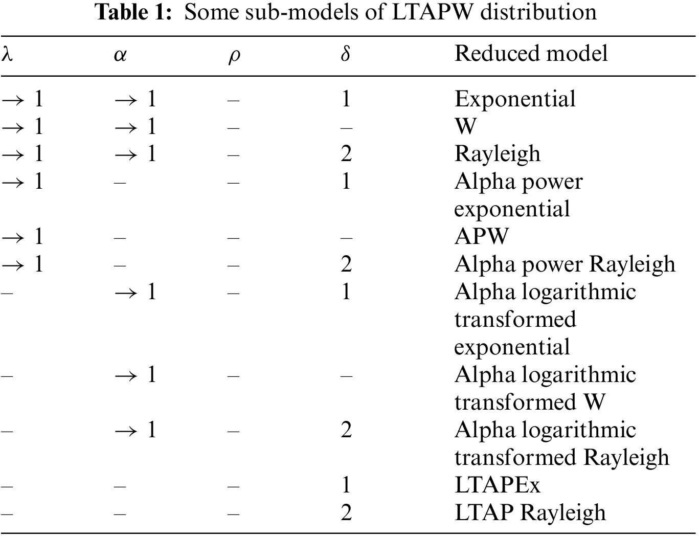
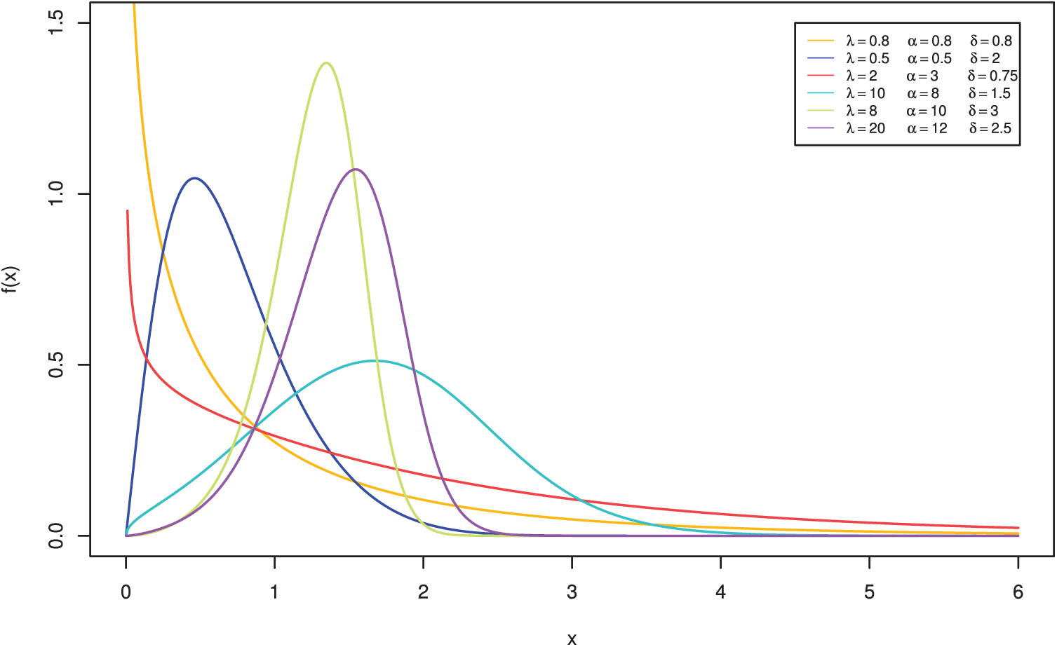
Figure 1: Different plots of the LTAPW distribution’s PDF
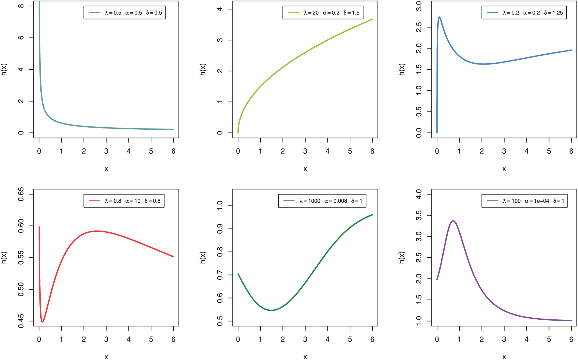
Figure 2: Different plots of the LTAPW distribution’s HRF
Throughout the paper, we will use
For estimation (for instance, quantile estimators) and simulation, quantiles are essential. For the LTAPW distribution, the
By substituting
By putting
In this subsection, we offer some mixture expressions for the PDF and CDF of the LTAPW distribution. Employing the generalized binomial expansion and the power series given, respectively, by
and
Applying (12) and (13) to the PDF in (6), then the following is a useful linear expression for the PDF of the LTAPW distribution:
where
By integrating (14), the linear expression for the CDF of the LTAPW distribution given by (5), can be obtained as
where
Moments are crucial to statistics and the use of statistics. Moments can be utilized to examine a probability distribution’s tendency, variation, and symmetry, among other essential aspects. The
where
and
Incomplete moments (IMs), moment generating functions (MGF), characteristic function (CF), and conditional moments (CMs) are four different forms of moments for the LTAPW distribution which can be expressed according to the following theorem:
Theorem. If
1. The
where
2. The MGF of X is
where
3. The CF of X is
4. The
where
2.4 Mean Deviations, Bonferroni and Lorenz Curves
The mean deviations from the mean and median are applications of the IMs. They are employed to evaluate how far a population has spread from its center. The mean deviations from the mean and the median can be derived, respectively, as follows:
and
where
where
Moreover, Bonferroni and Lorenz curves, denoted by
where
2.5 Entropies of LTAPW Distribution
The amount of information that can be expected from a random variable is called entropy. In many fields, including physics, finance, statistics, chemistry, insurance and biological phenomena, estimating entropy is essential. Less information in a sample is directed to retaining higher entropy. For the LTAPW distribution, the Rényi entropy (RE), denoted by
Using series presented in (12) and (13), the RE in (18) can be written as follows:
where
and
Suppose that
where
where
In this case, the PDF of the
On the other hand, the CDF of the
The residual life (RL) function in reliability and life testing refers to the extra lifetime presumed that a component has stayed until time
Based on (5), (14) and applying the binomial expansion of
where
where
Using (5) and (14), it follows:
where
3 Maximum Likelihood Estimation
The MLEs of the different unknown parameters and the associated approximate confidence intervals (ACIs) using the asymptotic traits of the MLEs are discussed in this section. Let
The log-likelihood function of (23) is expressed as follows:
To get the MLEs of
and
It is clear that
where
and
As a result, the
where
The performance of the MLEs of the unknown parameters is examined in this section using simulation research based on 1000 samples generated from the LTAPW Distribution. The effectiveness of estimates is assessed in terms of various criteria, bias, root mean square error (RMSE) and interval length (IL), computed according to the following formulas:
and
where
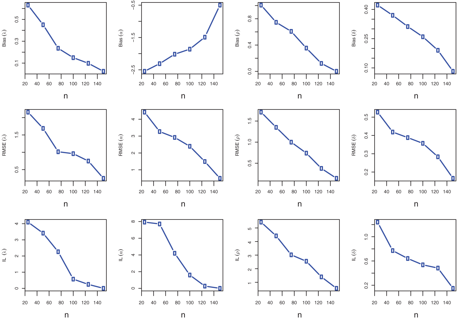
Figure 3: Bias, RMSE and ILs for
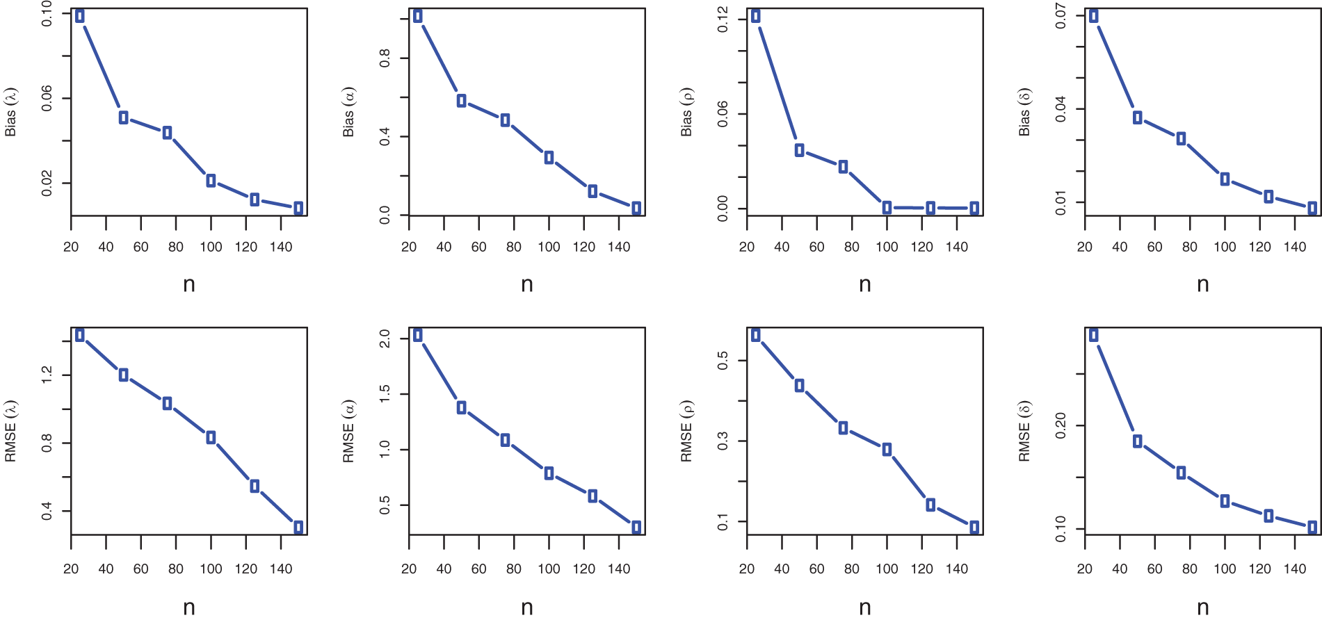
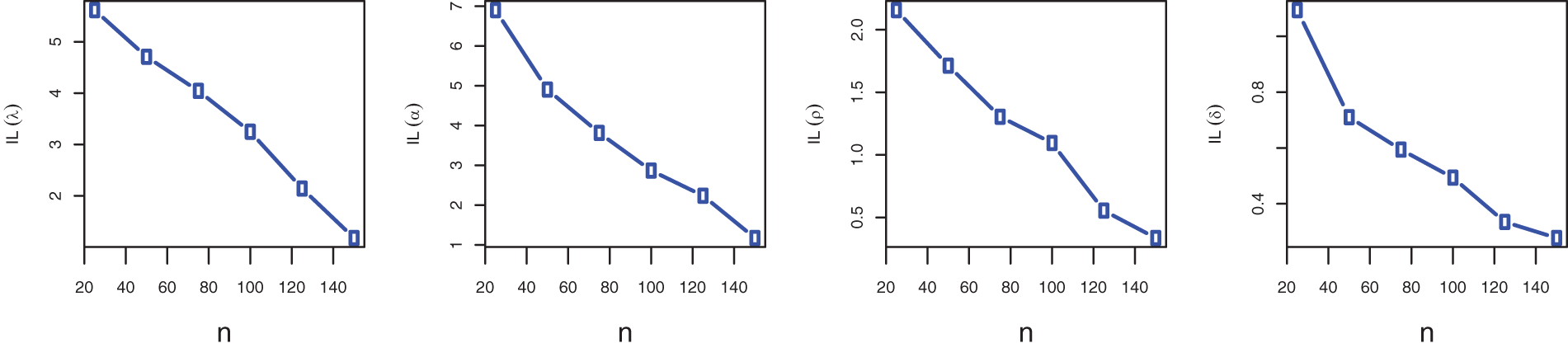
Figure 4: Bias, RMSE and ILs for

Figure 5: Bias, RMSE and IL for
To show the effectiveness of our offered LTAPW distribution, three actual data sets are taken into account in this part. The first set of data (Data I) details the COVID-19 patient fatality rates in Italy for 59 days from 27 February to 27 April 2020. This data set was used by Almongy et al. [15] and analyzed recently by El-Sagheer et al. [16]. The second data set (Data II) comprises 40 observations of the airborne communication transceiver’s active repair time, see for more details in Jorgensen [17] and Alotaibi et al. [18]. The lifespan (in years) of 40 patients with blood cancer (leukemia) from one of the Ministry of Health institutions in Saudi Arabia are included in the third data set (Data III) that was investigated in Al-Saiary et al. [19] and Klakattawi [20]. The actual data sets are displayed in Table 2. The box plots of the different data sets are displayed in Fig. 6. It shows that Data I and III are approximately symmetric, while Data II is positively skewed.
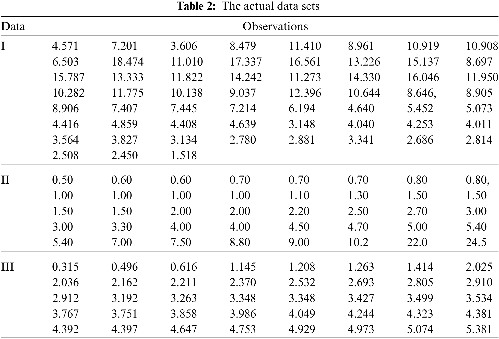

Figure 6: Box plots of various data sets
We compare the results of the proposed model with some of its sub-models namely, LTAPEx distribution proposed by Alotaibi et al. [13], APW distribution by Nassar et al. [5] and the traditional W distribution. The MLEs of the parameters of the LTAPW distribution and the other models for the given data sets along with their standard errors as well as the
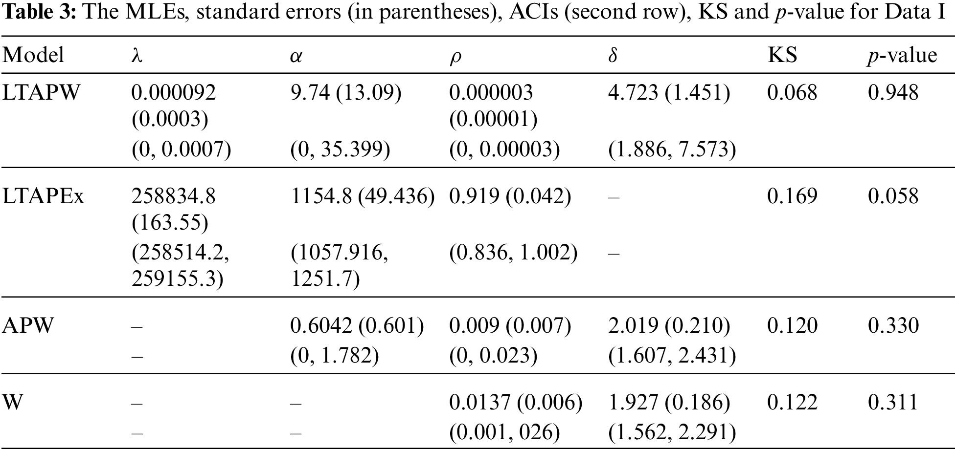


Figure 7: Histogram and fitted PDF, estimated and empirical RF and PP-plot of LTAPW distribution for Data I

Figure 8: Histogram and fitted PDF, estimated and empirical RF and PP-plot of LTAPW distribution for Data II

Figure 9: Histogram and fitted PDF, estimated and empirical RF and PP-plot of LTAPW distribution for Data III
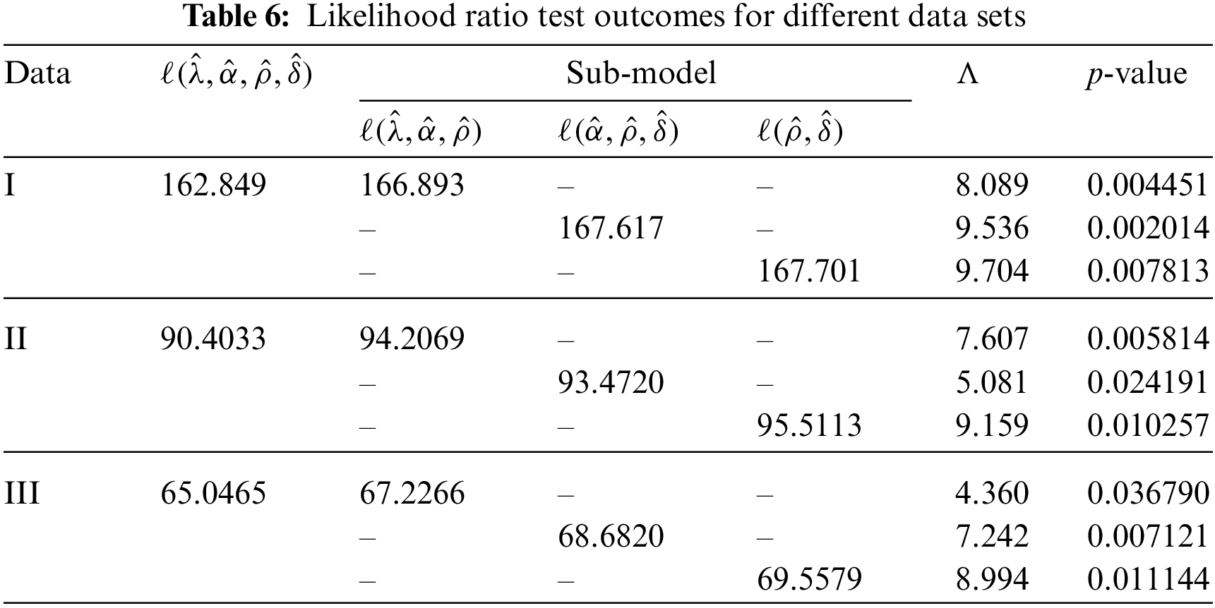
Since the LTAPEx, APW and W distributions can be derived as special cases of the LTAPW distribution, then we propose to consider the likelihood ratio test to examine the suitability of the considered sub-models against the LTAPW distribution. To perform the required tests, we need to obtain
In this paper, we present a new lifetime distribution called the logarithmic transformed alpha power Weibull distribution. The proposed model has one scale and three shape parameters and can model left-skewed, right-skewed, and approximately symmetric data. It contains many special sub-models including Weibull, exponential, and alpha power Weibull distributions. Besides the constant, decreasing, and increasing failure rate shapes as classical forms, it is able also to model the data sets with unimodal, bathtub, unimodal then bathtub, and bathtub then unimodal shapes. The main properties of the offered distribution are derived in detail, including mixture representation, quantile function, moments, entropies, order statistics and moments of residual life. The maximum likelihood procedure is employed to acquire the point and interval estimators of the parameters. Simulation research is conducted to evaluate the functionality of the unknown parameters. The efficiency of the estimates is evaluated based on bias, root mean square error and interval length. The simulation outcomes showed that the proposed estimates perform well in terms of minimum values of the considered criteria. Three applications are considered to demonstrate the usefulness of the suggested distribution in modeling real-world data. Also, the likelihood ratio test is considered to show the superiority of the new model over some of its sub-models, namely Weibull, alpha power Weibull and logarithmic transformed alpha power Weibull distributions. Due to the flexibility of the new distribution in modeling various types of data with different failure rates, we anticipate that the new distribution will find extensive use across a variety of fields. In future work, it is of interest to investigate the estimation problems of the proposed model based on censoring schemes. Also, one may compare the classical estimation methods of the unknown parameters, including least squares and maximum product of spacing methods, with the Bayesian estimation approach.
Acknowledgement: The authors would desire to express their appreciation to the editor and the three anonymous referees for useful guidance and helpful observations.
Funding Statement: The Deanship of Scientific Research (DSR) at King Abdulaziz University, Jeddah, Saudi Arabia has funded this project under Grant No. (G-102-130-1443).
Conflicts of Interest: The authors declare that they have no conflicts of interest to report regarding the present study.
References
1. Mudholkar, G. S., Srivastava, D. K. (1993). Exponentiated Weibull family for analyzing bathtub failure-rate data. IEEE Transactions on Reliability, 42(2), 299–302. [Google Scholar]
2. Marshall, A. W., Olkin, I. (1997). A new method for adding a parameter to a family of distributions with application to the exponential and Weibull families. Biometrika, 84(3), 641–652. [Google Scholar]
3. Cordeiro, G. M., Ortega, E. M., Nadarajah, S. (2010). The Kumaraswamy Weibull distribution with application to failure data. Journal of the Franklin Institute, 347(8), 1399–1429. [Google Scholar]
4. Abouelmagd, T. H. M., Al-mualim, S., Elgarhy, M., Afify, A. Z., Ahmad, M. (2017). Properties of the four-parameter weibull distribution and its applications. Pakistan Journal of Statistics, 33, 449–466. [Google Scholar]
5. Nassar, M., Alzaatreh, A., Mead, M., Abo-Kasem, O. (2017). Alpha power Weibull distribution: Properties and applications. Communications in Statistics-Theory and Methods, 46(20), 10236–10252. [Google Scholar]
6. Nassar, M., Afify, A. Z., Dey, S., Kumar, D. (2018). A new extension of Weibull distribution: Properties and different methods of estimation. Journal of Computational and Applied Mathematics, 336, 439–457. [Google Scholar]
7. Cordeiro, G. M., Afify, A. Z., Ortega, E. M. M., Suzuki, A. K., Mead, M. E. (2019). The odd Lomax generator of distributions: Properties, estimation and applications. Journal of Computational and Applied Mathematics, 347, 222–237. [Google Scholar]
8. Shakhatreh, M. K., Lemonte, A. J., Moreno-Arenas, G. (2019). The log-normal modified Weibull distribution and its reliability implications. Reliability Engineering & System Safety, 188, 6–22. [Google Scholar]
9. Shakhatreh, M. K., Lemonte, A. J., Cordeiro, G. M. (2020). On the generalized extended exponential-Weibull distribution: Properties and different methods of estimation. International Journal of Computer Mathematics, 97(5), 1029–1057. [Google Scholar]
10. Nassar, M., Afify, A. Z., Shakhatreh, M. K., Dey, S. (2020). On a new extension of Weibull distribution: Properties, estimation, and applications to one and two causes of failures. Quality and Reliability Engineering International, 36(6), 2019–2043. [Google Scholar]
11. Pappas, V., Adamidis, K., Loukas, S. (2012). A family of lifetime distributions. International Journal of Quality, Statistics, and Reliability, 2012(1), 1–6. [Google Scholar]
12. Mahdavi, A., Kundu, D. (2017). A new method for generating distributions with an application to exponential distribution. Communications in Statistics-Theory and Methods, 46(13), 6543–6557. [Google Scholar]
13. Alotaibi, R., Nassar, M. (2022). A new exponential distribution to model concrete compressive strength data. Crystals, 12(3), 431. [Google Scholar]
14. Cordeiro, G. M., Lemonte, A. J. (2013). On the Marshall-Olkin extended Weibull distribution. Statistical Papers, 54(2), 333–353. [Google Scholar]
15. Almongy, H. M., Almetwally, E. M., Aljohani, H. M., Alghamdi, A. S., Hafez, E. H. (2021). A new extended Rayleigh distribution with applications of COVID-19 data. Results in Physics, 23(60), 104012 [Google Scholar] [PubMed]
16. El-Sagheer, R. M., Almuqrin, M. A., El-Morshedy, M., Eliwa, M. S., Eissa, F. H. et al. (2022). Bayesian inferential approaches and bootstrap for the reliability and hazard rate functions under progressive first-failure censoring for coronavirus data from asymmetric model. Symmetry, 14(5), 956. [Google Scholar]
17. Jorgensen, B. (1982). Statistical properties of the generalized inverse gaussian distribution. New York, USA: Springer. [Google Scholar]
18. Alotaibi, R., Okasha, H., Nassar, M., Elshahhat, A. (2022). A novel modified alpha power transformed Weibull distribution and its engineering applications. Computer Modeling in Engineering & Sciences, 135(3), 2065–2089. https://doi.org/10.32604/cmes.2023.023408 [Google Scholar] [CrossRef]
19. Al-Saiary, Z. A., Bakoban, R. A. (2020). The Topp-Leone generalized inverted exponential distribution with real data applications. Entropy, 22(10), 1144 [Google Scholar] [PubMed]
20. Klakattawi, H. S. (2022). Survival analysis of cancer patients using a new extended Weibull distribution. PLoS One, 17(2), e0264229 [Google Scholar] [PubMed]
Cite This Article
 Copyright © 2023 The Author(s). Published by Tech Science Press.
This work is licensed under a Creative Commons Attribution 4.0 International License , which permits unrestricted use, distribution, and reproduction in any medium, provided the original work is properly cited.
 Downloads
 Citation Tools