An Efficient Numerical Scheme for Biological Models in the Frame of Bernoulli Wavelets

1  Introduction

The evolution and development of the contemporary world can’t be separated from mathematics. Mathematics is related to nearly all human movement. A mathematical model is a helpful tool for solving real-life problems. Application to determine the blowout of the transmittable disease model in a particular region is one of the finest examples of this. Researchers started studying biological systems over many years. These biological systems are usually in the form of a system of coupled ordinary differential equations. Only a few of these biological models have exact solutions and are typically intricate. Therefore, there is a necessity for a decent approximated solution. Numerical methods are often the best choice for these systems as they will produce nonnegative solutions and describe these systems’ dynamic behavior. In these systems, the specified variables commonly represent nonnegative quantities, such as the size of the population, number of chemical components, concentration, and physical properties.

Due to technological advances in medical research, like vaccination and antibodies to viral diseases, it was predictable that the spread of transmissible diseases would be overcome. But it didn’t. The reason is that most of the developed countries have concentrated their research on cancer and other incurable diseases. Consequently, infectious diseases still cause intense suffering and a high mortality rate. Ebola, Yellow fever, Aids, Malaria, and other names have left a deep scar on the history of humanity forever.

Among all the above viruses, Dengue fever is mainly extensive in Southern Asia. Dengue is a complicated disease transmitted to humans through mosquitoes belonging to the Genus Aedes. They exist in two forms: Dengue Haemorrhagic Fever (DHF) and classical dengue. The furthermost problematic characteristic of dengue is that it can be triggered by four different serotypes known as DEN1, DEN2, DEN3, and DEN4. If the person is infected with any one of the types will never be infected by the same type again, a phenomenon called homologous immunity. Though, once the human is infected by any of the above types, in about 12 weeks, he loses immunity to the other types, known as heterologous immunity.

The mathematical modelling of Dengue fever is [1]:

dS(t)dt=μh(1−S(t))−αS(t)R(t)dI(t)dt=αS(t)R(t)−βI(t)dR(t)dt=γ(1−R(t))I(t)−δ1R(t)}(1)

where S(t) represents the potential victims of the dengue virus (Suspectable), I(t) represents the people who are already infected with dengue (Infected) and R(t) represents the recovered patients from the dengue virus (Recovered), μh is the natural death rate of the human population, βh is the rate of infection in the human population, α is the vaccine efficacy coefficient, γ is the recovery rate, δ1 is the number of death among the susceptible population. Some of the numerical techniques implemented for the SIR Model of Dengue fever are: M. Khalid et al. proposed a new approach called the Perturbation Iteration Algorithm (PIM) [1]. Rangkutti et al. implemented Homotopy Perturbation method and Variational Iteration method [2]. Mungkasi proposed an Improved Variational Iteration method for the SIR Model of Dengue [3]. Umar et al. proposed a Stochastic numerical computing scheme with artificial neural networks [4]. Lede et al proposed Euler and Heun methods [5].

Coronavirus disease (COVID-19) is a new disease generated by a recently recognized virus, Severe Acute Respiratory Syndrome Coronavirus 2 (SARS-CoV-2) was first reported in Wuhan, China, in December 2019 and was declared a pandemic by the World Health Organisation (WHO) on 11th March 2020. The transmission of viruses in human beings from the compartment of S(t) to the I(t) and from the compartment of I(t) to the R(t) can be described by the set of three systems of non-linear ordinary differential equations with only two constraint approximations.

The simple SIR model for COVID-19 virus transmission is [6]:

dS(t)dt=−α0S(t)I(t)dI(t)dt=α0S(t)I(t)−α1I(t)dR(t)dt=α1I(t)}(2)

where S(t) represents the fraction of Susceptible persons, I(t) represents the fraction of Infected persons, R(t) represents the fraction of recovered persons, α0 is the infection rate and α1 is the removal rate. Some numerical techniques implemented for the Coronavirus model are: Suba et al. implemented the current mathematical models and numerical simulation of the SIR Model for coronavirus (COVID-19) [6], Zeb et al. presented the mathematical model for coronavirus disease and a numerical solution is obtained by the nonstandard finite difference (NSFD) scheme [7]. Annas et al. proposed a stability analysis and numerical simulation of the SIR model for the COVID-19 pandemic [8]. ud Din et al. implemented the numerical simulation using the Nonstandard finite difference (NSFD) scheme [9]. Shahrear et al. imposed a mathematical analysis of the coronavirus outbreak [10].

TB (Tuberculosis) is an infectious epidemic usually produced by bacteria named Mycobacteria Tuberculosis which outbreaks human lungs. In some situations, it can also affect the other parts of the body, like the kidney, spine, skin, brain, etc. TB is spread from an infected person to an average person through air droplets that are contaminated with germs. A person will become easily contaminated when they breathe a few microorganism germs. TB-infected individuals can be diagnosed through blood and skin tests. TB creates a high risk for HIV and diabetes patients. The signs of the live TB disease include a cough that tests for more than three weeks, loss in weight, coughing up blood, felt tiredness, exhaustion, chest pain, and night sweats. The World Health Organisation states that Tuberculosis has infected one-third of the world population. In 2018, an estimated 10 million new cases of TB disease were described, and a total of 1.5 million people died from TB worldwide. Apart from this, 1.2 million estimated TB patients died HIV-negative, and 0.25 million died HIV-positive in 2018. A large number of TB patients died in the region of low- and middle-income countries (LMICs), including India (27%), Nigeria (4%), Indonesia (8%), Pakistan (6%), Philippine (6%), Bangladesh (4%) and South Africa (24%). Southeast Asia (44%) has reported most of the occurred cases of TB [11], even though TB is a treatable transferrable disease using drug therapy [12].

The SIR Model of Tuberculosis is as follows [13]:

dS(t)dt=A−μS(t)−rI(t)S(t)NdI(t)dt=rI(t)S(t)N−(μ+a)I(t)dR(t)dt=aI(t)−μR(t)}(3)

where N = S + I + R, S(t) is the number of vulnerable individuals in the population at the time t, I(t) is the number of infected individuals in the population at time t, R(t) is the number of individuals who recovered in the population at time t, r is the rate of transmission of disease from susceptible become infectious (0≤r≤1), a is the rate of recovery from infectious to recovered, A is the initial value, μ is the death rate. Some of the numerical techniques implemented for the Tuberculosis model are: Side et al. proposed a numerical solution for transmission of Tuberculosis by the Runge Kutta method [13]. Kanwal et al. implemented the three numerical techniques, which are the nonstandard finite difference (NSFD), Runge-Kutta method of order 4 (RK4), and forward Euler (FD) scheme [14]. Ibrahim et al. presented Homotopy Analysis method [15]. Das et al. studied the mathematical transmission analysis of the model [16]. Ningsi et al. proposed Variational Iteration method [17]. The epidemic model of childhood disease and the fractional model of vector-borne diseases and tumor invasion and metastasis have been studied in [18–20]. The massive stirring and non-linear liénard differential models have been investigated in [21,22].

The subject of wavelet appeared in the mid-1980s, influenced by ideas from both pure and applied mathematics. In 1807, Joseph Fourier developed a method for representing signals with a series of coefficients based on an analysis function. He laid the mathematical basis from which the wavelet theory was developed. The first to mention wavelets was Alfred Haar in 1909 in his Ph.D. thesis. The wavelet theory is a relatively renewed and emerging theory in mathematical research. wavelet analysis is a great tool that significantly impacts study and engineering. The primary criteria that draw researchers to the wavelet are orthogonality and effective localization. With the help of wavelets that are mathematical operations, data may be divided into several frequency components, each of which can then be analyzed at a different resolution. It is possible to employ wavelets as a mathematical tool to extract information from a variety of data formats. Wavelets are based on the fundamental theory of expressing a complicated function by a set of self-similar functions by super positioning, a principle introduced by Joseph Fourier in the 1800s. They have advantages over traditional Fourier methods in analyzing physical situations where the signal contains discontinuities and sharp spikes. Bernoulli wavelet is one of the continuous basis wavelets with orthogonality, compact support, etc. Due to these properties, wavelet methods yield better accuracy in the solution. Some of the problems tackled by the wavelets collocation method on mathematical models arising in science and technology are Laguerre, Hermite, and Legendre wavelets methods to solve some of the mathematical models [23–31], the Bernoulli wavelets scheme for fractional delay differential equations [32] and Fractional pantograph differential equations [33], Non-linear second-order Lane–Emden pantograph delay differential mode solved by Bernoulli wavelets [34], Fractional Riccati differential equation [35], Fractional order model of novel coronavirus outbreak [36], non-linear singular Lane–Emden type equations arising in astrophysics are successfully tackled by Bernoulli wavelet [37], Designing of Morlet wavelet as a neural network for a novel prevention category in the HIV system [38], Bernstein wavelets for SIR epidemic infectious model [39], Bernstein wavelets for predator-prey dynamical system [40], Bernoulli wavelets collocation method newly applied for different mathematical problems [41–44], Bernoulli wavelets for Glucose-Insulin regulatory dynamical system [45], and Fibonacci wavelets [46]. The results of BWCS are compared with other methods, like the Runge Kutta method and ND Solver. The results obtained in this paper are new and do not exist in the literature. This paper is organized as follows: Section 2 gives the preliminaries of the Bernoulli wavelet, and its properties, Section 3 deals with the functional matrix of the Bernoulli wavelet, and Section 4 reflects the method of solution and application of the proposed method deals with Section 5. Lastly, Section 6 presents conclusions on the new BWCS.

2  Preliminaries of Bernoulli Wavelet and Its Properties

The Bernoulli wavelets are defined as [47]:

θn,m(x)={2k−12bm~(2k−1x−n^),n^2k−1≤x<n^+12k−10,Otherwise

with

bm~(x)={1,m=01(−1)m−1(m !)2(2 m) !a2 mbm(x), m>0

where m=0,1,2,…,M−1,n=1,2,…, 2k−1.

The coefficient 1(−1)m−1(m !)2(2m)!a 2m is intended for normality, the dilation parameter is f=2−(k − 1) and the translation parameter  g=n^ 2−( k−1 ). Here, bm(x) are the well-known Bernoulli polynomials of order m, which can be described as  bm(x)=∑i=0m(mi)am−ixi, where  ai, i=0 , 1 ,…, m are Bernoulli numbers. Those numbers are a sequence of signed rational numbers that rise within the series enlargement of trigonometric capabilities and can be defined by employing the identity,

 xex−1=∑i=0∞a ix ii !

Some initial Bernoulli numbers are:

a0=1,a1=−12,a2=16,a4=−130,a6=142,a8=−130,a10=566,a12=−6912730,a14=76,a16=−3617510,a18=43867798,…

with a2i+1=0, i= 1, 2, 3,…

Some initial Bernoulli polynomials are:

b0=1,b1=−12+x,b2=16 − x+x2,b3=x2−3x2+x3,

b4=−130+x2−2x3+x4,b5=−x6+5x33−5x42+x5,

b6=142−x22+5x42−3x5+x6,b7=x6−7x36+7x52−7x62+x7,

b8=−130+2x23−7x43+14x63−4x7+x8,b9=−3x10+2x3−21x55+6x7−9x82+x9,

b10=566−3x22+5x4−7x6+15x82−5x9+x10,…

Theorem 1 [48]: Let H be a Hilbert space and W be a closed subspace of H such that dim⁡W<∞ and {w1,w2,…,wn} is any basis for W. Let g be an arbitrary element in H and g0 be the unique best approximation to g out of W. Then,

||g−g0||2=Gg, where Gg=(Z(g,w1,w2,…wn)Z(g,w1,w2,…wn))12 and Z is introduced inas below:

Z(g,w1,w2,…wn)=|<g,g><g,w1>…<g,wn><w1,g><w1,w1>…<w1,wn>…………<wn,g><wn,w1>…<wn,wn>|

Theorem 2 [48,49]: Let L2[0,1] be the Hilbert space generated by the Bernoulli wavelet basis. Let η(x) be the continuous bounded function in L2[0,1]. Then the Bernoulli wavelet expansion of η(x) converges to it.

3  Functional Matrix of Bernoulli Wavelets

Some Bernoulli wavelet basis at k=1 are [48]:

θ1,0(x)=1

θ1,1(x)=3(−1+2x)

θ1,2(x)=5(1−6x+6x2)

θ1,3(x)=210(x−3x2+2x3)

θ1,4(x)=1021(−130+x2−2x3+x4)

θ1,5(x)=4625(−x+10x3−15x4+6x5)

θ1,6(x)=1430691(1−21x2+105x4−126x5+42x6)

θ1,7(x)=21437(x−7x3+21x5−21x6+6x7)

θ1,8(x)=72933617(−1+20x2−70x4+140x6−120x7+30x8)

θ1,9(x)=1939938219335(−3x+20x3−42x5+60x7−45x8+10x9)

θ1,10(x)=22125970174611(566−3x22+5x4−7x6+15x82−5x9+x10)

θ1,11( x )=2676039854513(5x−33x3+66x5−66x7+55x9−33x10+6x11)

θ10( x )=[θ1,0(x),θ1,1(x),θ1,2(x),θ1,3(x),θ1,4(x),θ1,5(x),θ1,6(x),θ1,7(x),θ1,8(x),θ1,9(x)]T

On integrating the above basis concerning x limit from 0 to x, and then expressing it as a linear combination of Bernoulli wavelet basis, we obtain

∫0xθ1,0(x)dx=[1212300000000]θ10( x )

∫0 xθ1,1 (x)dx=[− 123012150000000]θ10(x)

∫0xθ1,2(x)dx=[000142000000]θ10(x)

∫0xθ1,3(x)dx=[7230000121000000]θ10(x)

∫0xθ1,4(x)dx=[0000053220000]θ10(x)

∫0xθ1,5(x)dx=[−112100000069110273000]θ10(x)

∫0xθ1,6(x)dx=[000000035138200]θ10(x)

∫0xθ1,7(x)dx=[14320700000003617203570]θ10(x)

∫0xθ1,8(x)dx=[0000000002193353962122]θ10(x)

∫0xθ1,9(x)dx=[−1469652895222000000000]θ10(x)+122227710482537θ1,10(x)

Hence,

∫oxθ(x)dx=฿10×10 θ10(x)+θ10¯(x)(4)

where,

฿10×10=[1212300000000−12301215000000000014200000072300001210000000000053220000−112100000069110273000000000035138200143207000000036172035700000000002193353962122−1469652895222000000000]

θ10¯(x)=[000000000122227710482537θ1,10(x)]

In general, the Bernoulli wavelet’s first integration can be depicted as; ∫ 0xθ(x)dx=฿n×nθn(x)+θn¯(x).

4  Bernoulli Wavelet Method

Here, we would like to bring the solution of the Dengue Fever Model (1.1) to the Bernoulli wavelet space. Assume that,

dSdt=ATθ(t)(5)

dIdt=BTθ(t)(6)

dRdt=CTθ(t)(7)

BT=[b1,0,…b1,M−1,b2,0,…b2,M−1,b2k−1,0,…b2k−1,M−1]

CT=[c1,0,…c1,M−1,c2,0,…c2,M−1,c2k−1,0,…c2k−1,M−1]

θ(t)=[θ(t)1,0,…θ(t)1,M−1,θ(t)2,0,…θ(t)2,M−1,θ(t)2k−1,0,…θ(t)2k−1,M−1]

Integrate Eqs. (5)–(7) concerning ‘t’ from ‘0’ to ‘t’. We get

S(t)=S(0)+∫0tAT θ(t)dtA

I(t)=I(0)+∫0tBT θ(t)dt

R(t)=R(0)+∫0tCT θ(t)dt

From the Eq. (4) along with initial conditions expressed in terms of θ (t). We obtain

S(t)=DTθ(t)+AT[฿ θ(t)+θ¯ (t)]I(t)=ETθ(t)+BT[฿ θ(t)+θ¯ (t)]R(t)=FTθ(t)+CT[฿ θ(t)+θ¯ (t)]}(8)

where D, E, and F are the known vectors. Substitute Eqs. (5)–(8) in (1) we get

ATθ(t)=μh(1−DTθ(t) +AT[฿ θ(t)+θ¯ (t)])−α(DTθ(t) +AT[฿ θ(t)+θ¯ (t)])(FTθ(t) +CT[฿ θ(t)+θ¯ (t)]) BTθ(t)=α(DTθ(t) +AT[฿ θ(t)+θ¯ (t)])(FTθ(t) +CT[฿ θ(t)+θ¯ (t)])−β(ETθ(t)+BT[฿ θ(t)+θ¯ (t)])CTθ(t)=γ(1−FTθ(t) +CT[฿ θ(t)+θ¯ (t)])(ETθ(t)+BT[฿ θ(t)+θ¯ (t)])−δ(FTθ(t) +CT[฿ θ(t)+θ¯ (t)])}(9)

Now collocate each Eq. (9) with the following grid points:

ti=2i−12M,i=1,2,…,M

We get a non-linear system of algebraic equations from the above procedure:

ATθ(ti)=μh(1−DTθ(ti) +AT[฿ θ(ti)+θ¯ (ti)])−α(DTθ(ti) +AT[฿ θ(ti)+θ¯ (ti)])(FTθ(ti) +CT[฿ θ(ti)+θ¯ (ti)])BTθ(ti)=α(DTθ(ti) +AT[฿ θ(ti)+θ¯ (ti)])(FTθ(ti) +CT[฿ θ(ti)+θ¯ (ti)])−β(ETθ(ti)+BT[฿ θ(ti)+θ¯ (ti)])CTθ(ti)=γ(1−FTθ(ti) +CT[฿ θ(ti)+θ¯ (ti)])(ETθ(ti)+BT[฿ θ(ti)+θ¯ (ti)])−δ(FTθ(ti) +CT[฿ θ(ti)+θ¯ (ti)])}(10)

Eq. (10) can be solved by Newton’s Raphson method. This yields the values of Bernoulli’s unknown coefficients and substituting these values on (8) yields Bernoulli’s wavelet-based numerical solutions for the defined model.

Next, we would like to bring the solution of the Coronavirus Model (2) to the Bernoulli wavelet space. Substitute Eqs. (5)–(8) in (2) we get

ATθ(t)=−α0(DTθ(t) +AT[฿ θ(t)+θ¯ (t)])(ETθ(t)+BT[฿ θ(t)+θ¯ (t)])BTθ(t)=α0(DTθ(t) +AT[฿ θ(t)+θ¯ (t)])(ETθ(t)+BT[฿ θ(t)+θ¯ (t)])−α1(ETθ(t)+BT[฿θ(t)+θ¯ (t)])CTθ(t)=α1(ETθ(t)+BT[฿ θ(t)+θ¯ (t)])}(11)

Now collocate each equation in (11) with the following grid points:

ti=2i−12M,i=1,2,…,M

We get a non-linear system of algebraic equations from the above procedure:

ATθ(ti)=−α0(DTθ(ti) +AT[฿ θ(ti)+θ¯ (ti)])(ETθ(ti)+BT[฿ θ(ti)+θ¯ (ti)])BTθ(ti)=α0(DTθ(ti) +AT[฿ θ(ti)+θ¯ (ti)])(ETθ(ti)+BT[฿ θ(ti)+θ¯ (ti)])−α1(ETθ(ti)+BT[฿ θ(ti)+θ¯ (ti)])CTθ(ti)=α1(ETθ(ti)+BT[฿ θ(ti)+θ¯ (ti)])}(12)

Eq. (12) can be solved by Newton’s Raphson method. This yields the values of Bernoulli’s unknown coefficients, after substituting these values on (8) delivers Bernoulli’s wavelet-based numerical solutions for the defined model.

Next, we would like to bring the solution of the Tuber coulis model (3) to the Bernoulli wavelet space. Substitute Eqs. (5)–(8) in (3) we get

ATθ(t)=A−μ(DTθ(t) +AT[฿ θ(t)+θ¯ (t)])−rN(ETθ(t)+BT[฿ θ(t)+θ¯ (t)])(DTθ(t) +AT[฿ θ(t)+θ¯ (t)])BTθ(t)=rN(ETθ(t)+BT[฿ θ(t)+θ¯ (t)])(DTθ(t) +AT[฿ θ(t)+θ¯ (t)])(μ+a)(ETθ(t)+BT[฿ θ(t)+θ¯ (t)])CTθ(t)=a(ETθ(t)+BT[฿ θ(t)+θ¯ (t)])−μ(FTθ(t) +CT[฿ θ(t)+θ¯ (t)])}(13)

Now collocate each equation in (13) with the following grid points:

ti=2i−12M,i=1,2,…,M

We get a non-linear system of algebraic equations from the above procedure:

ATθ(ti)=−α0(DTθ(ti) +AT[฿ θ(ti)+θ¯ (ti)])(ETθ(ti)+BT[฿ θ(ti)+θ¯ (ti)])BTθ(ti)=α0(DTθ(ti) +AT[฿ θ(ti)+θ¯ (ti)])(ETθ(ti)+BT[฿ θ(ti)+θ¯ (ti)])−α1(ETθ(ti)+BT[฿ θ(ti)+θ¯ (ti)])CTθ(ti)=α1(ETθ(ti)+BT[฿ θ(ti)+θ¯ (ti)])}(14)

Eq. (14) can be solved by Newton’s Raphson method. This yields the values of unknown coefficients, after substituting these values on (8) produces Bernoulli’s wavelet-based numerical solutions for the defined model.

5  Numerical Implementation of the Biological Models

5.1 SIR Model of Dengue Fever [1]

Here we present our computational results and provide a discussion of the results. Considering the mathematical model (1) with the initial conditions: S(0)= 50708225071126 , I(0) =3045071126, R(0)=0.01 with parameter values α=0.006, β=0.333333, γ=0.375, δ1=0.02941, μh=0.0045. We obtained the BWCS solution and compared it with the Runge-Kutta and ND Solver solutions. Tables 1–3 reveal that the solutions obtained from the BWCS are accurate and yields better approximations than the Runge-Kutta method. Also in these tables, the absolute error (AE) of the proposed method is compared with the Runge-Kutta method and ND Solver. Also, absolute error is reduced by increasing the value of M (size of the operational matrix) which is shown in Tables 4–6. The solution obtained from the proposed method, Runge Kutta method, and ND Solver are drawn in Figs. 1–3. It clearly shows that solutions obtained from the proposed method are much closer to the ND solver solution. The absolute error of the proposed method and the Runge Kutta method with the ND Solver are compared graphically in Figs. 4–6 due to the non-availability of the exact solution. The flat line in the graph suggests that the developed scheme (BWCS) obtains the consistent absolute error at all the points in the given interval and also gives a better approximation than the Runge Kutta method.

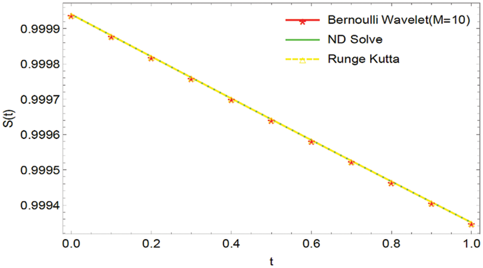
Figure 1: Graphical comparison of the BWCS solution, Runge-Kutta method solution with ND Solver solution for S(t)

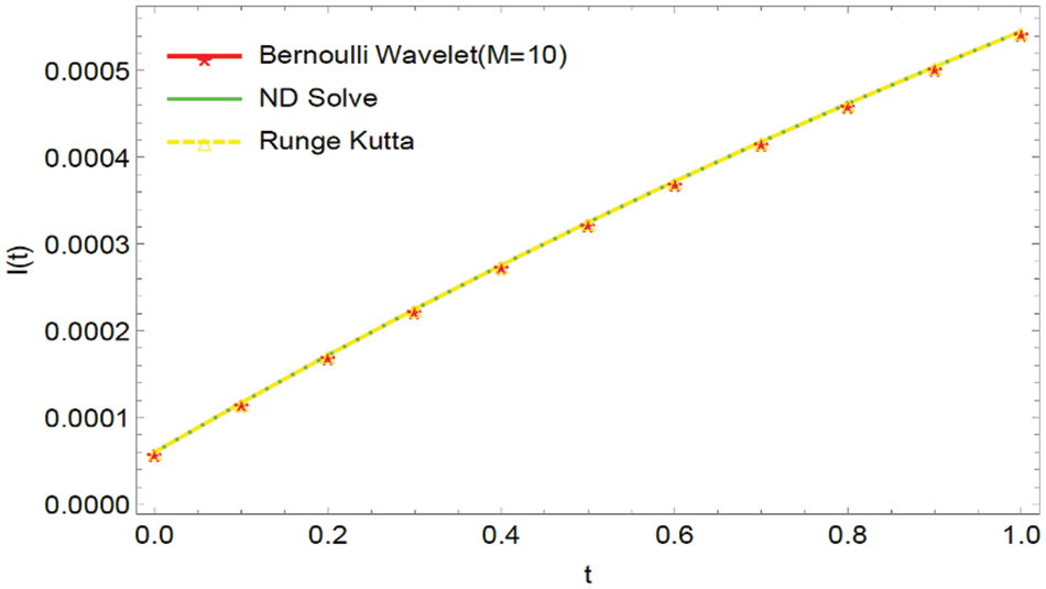
Figure 2: Graphical comparison of the BWCS solution, Runge-Kutta method solution with ND Solver solution for I(t)

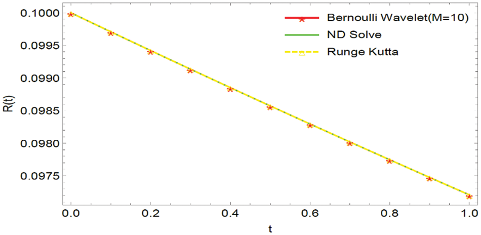
Figure 3: Graphical comparison of the BWCS, Runge-Kutta method solution with ND Solver solution for R(t)

Figure 4: Graphical representation of Absolute Errors (AE) for S(t)

Figure 5: Graphical representation of Absolute Errors (AE) for I(t)

Figure 6: Graphical representation of Absolute Errors (AE) for R(t)

5.2 Sir Model of COVID-19 Virus

Here we are considering the mathematical model of the COVID-19 virus (2) with the initial conditions: S(0)=0.999, I(0) =0.001, R(0)=0 with the parameter values α0=0.8, α1=0.1. We obtained the solution by the proposed method and compared it with the Runge-Kutta method and ND Solver solutions. Tables 7–9 reveal that the solutions obtained from the BWCS are accurate and yield better approximations than the Runge Kutta method. Also, absolute error is reduced by increasing the value of M which is shown in Tables 10–12. Figs. 7–9 clearly show that solutions obtained from the proposed method are much closer to the ND solver solution than the Runge-Kutta method. The present model has no exact solution, therefore, the absolute error of the proposed method and the Runge Kutta method compared with the NDSolver are shown graphically in Figs. 10–12. The flat line in the graph suggests that the developed scheme (BWCS) obtains the consistent absolute error at all the points in the given interval and also it gives a better approximation than the Runge Kutta method.

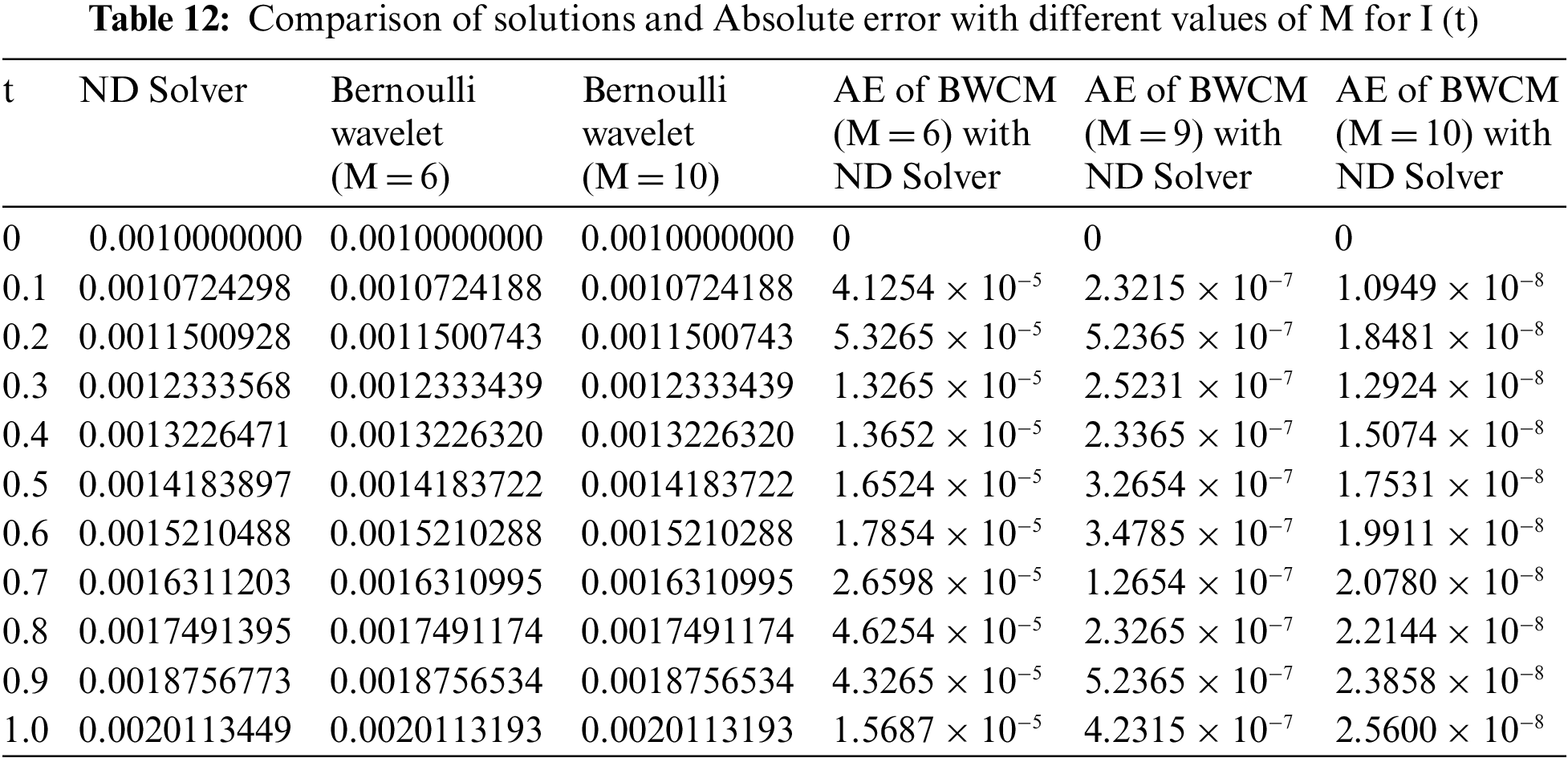
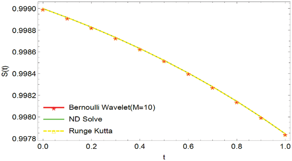
Figure 7: Graphical comparison of the BWCS solution, Runge-Kutta method solution with ND Solver solution for S(t) of the model (2)

Figure 8: Graphical comparison of the BWCS solution, Runge-Kutta method solution with ND Solver solution for I(t) of the model (2)

Figure 9: Graphical comparison of the BWCS solution, Runge-Kutta method solution with ND Solver solution for R(t) of the model (2)

Figure 10: Graphical representation of Absolute Errors (AE) for S(t)

Figure 11: Graphical representation of Absolute Errors (AE) for I(t)

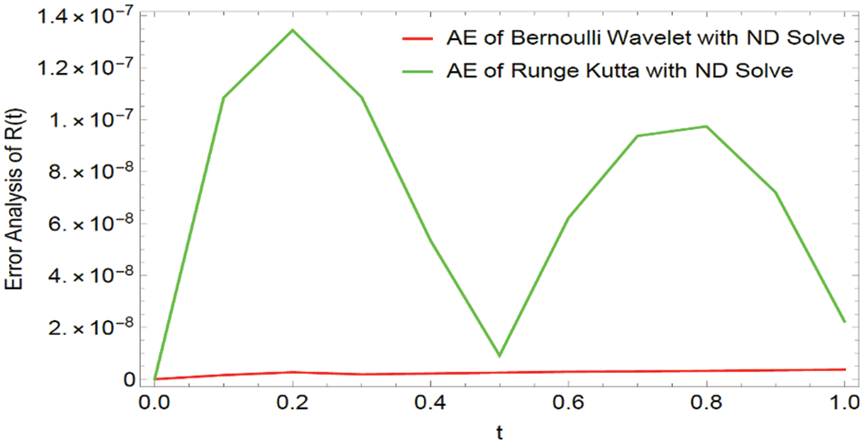
Figure 12: Graphical representation of Absolute Errors (AE) for R(t)

5.3 SIR Model for Transmission of Tuberculosis

In this section, we are considering the mathematical model for transmission of Tuberculosis (3) with the initial conditions: S(0)=14460931449401 , I(0) =18851449401, R(0)=14231449401 with the parameter values r=12, a=19, μ=0.001167, N=A=1449401. We obtained the solution from the BWCS and compared it with the Runge-Kutta method and ND Solver solutions. Tables 13–15 reveal that the solutions obtained from the BWCS are accurate and yield better approximations than the Runge-Kutta method. Also, absolute error is reduced by increasing the value of M which is shown in Tables 16–18. Figs. 13–18 clearly show that solutions obtained from the proposed method are much closer to the ND solver solution. The absolute error of the proposed method and the Runge Kutta method with the ND Solver are compared graphically in Figs. 16–18.

Figure 13: Graphical comparison of the BWCS, Runge-Kutta method solution with ND Solver solution for S(t)

Figure 14: Graphical comparison of the BWCS solution, Runge-Kutta method solution with ND Solver solution for I(t)

Figure 15: Graphical comparison of the BWCS solution, Runge-Kutta method solution with ND Solver solution for R(t)

Figure 16: Graphical representation of Absolute Errors (AE) for S(t)

Figure 17: Graphical representation of Absolute Errors (AE) for I(t)

Figure 18: Graphical representation of Absolute Errors (AE) for R(t)

6  Conclusion

In this article, we primarily concentrated on the numerical computations of three biological models: the Dengue fever model, the COVID-19 model, and the transmission of Tuberculosis model. We developed the functional integration matrix for the Bernoulli wavelet and generated a novel technique called BWCS. We used this functional matrix to estimate the mathematical model’s numerical solution, which is in the form of a non-linear system of ordinary differential equations. Our numerical results are compared with the Runge-Kutta method and ND solver solution through tables and Figures. Tables and Figures exposed the efficiency of our projected approach and compared it with different techniques. The received computational result indicates that our projected procedure is valuable and specific in contrast with other techniques. Also, we have introduced some theorems on convergence analysis. Tables 1–9 reveal that the BWCM solution is better than the Runge-Kutta method solution as compared with the ND solver solution. Figs. 1–3, 7–9, and 13–15 show that the BWCS solution is very close to the ND solver solution. Figs. 4–6, 10–12, and 16–18 reveal that the absolute error of the proposed method is better than the absolute error of the Runge-Kutta method when compared with the ND solver solution. Tables and Figures reveal that the BWCS converges rapidly compared to the Runge-Kutta method. This concludes that the developed strategy is a well-suited technique for the numerical approximations of biological models.

Acknowledgement: Authors thank editors and reviewers for helping the enrichment of this article. Also, Kumbinarasaiah S thanks Bangalore University for its support.

Funding Statement: The authors received no specific support for this study.

Conflicts of Interest: The authors declare that they have no conflicts of interest to report regarding the present study.

REFERENCES

1. Khalid, M., Sultana, M., Khan, F. S. (2015). Numerical solution of SIR model of dengue fever. International Journal of Computer Applications, 118(21). [Google Scholar]

2. Rangkuti, Y. M., Side, S., Noorani, M. S. M. (2014). The numerical analytic solution of SIR model of dengue fever disease in South Sulawesi uses homotopy perturbation and variational iteration methods. Journal of Mathematical and Fundamental Sciences, 46(1), 91–105. [Google Scholar]

3. Mungkasi, S. (2020). Improved variational iteration solutions to the SIR model of dengue fever disease for the case of South Sulawesi. Journal of Mathematical & Fundamental Sciences, 52(3), 297–311. [Google Scholar]

4. Umar, M., Sabir, Z., Raja, M. A. Z., Sánchez, Y. G. (2020). A stochastic numerical computing heuristic of SIR nonlinear model based on dengue fever. Results in Physics, 19, 103585. [Google Scholar]

5. Lede, Y. K., Mungkasi, S. (2019). Performance of the Runge-Kutta methods in solving a mathematical model for the spread of dengue fever disease. AIP Conference Proceedings, 2202, 020044. [Google Scholar]

6. Suba, M., Shanmugapriya, R., Balamuralitharan, S., Joseph, G. A. (2020). Current mathematical models and numerical simulation of sir model for coronavirus disease-2019 (COVID-19). European Journal of Molecular & Clinical Medicine, 7(5), 41–54. [Google Scholar]

7. Zeb, A., Alzahrani, E., Erturk, V. S., Zaman, G. (2020). Mathematical model for coronavirus disease 2019 (COVID-19) containing isolation class. BioMed Research International, 2020, 3452402. [Google Scholar] [PubMed]

8. Annas, S., Pratama, M. I., Rifandi, M., Sanusi, W., Side, S. (2020). Stability analysis and numerical simulation of SEIR model for pandemic COVID-19 spread in Indonesia. Chaos, Solitons & Fractals, 139, 110072. [Google Scholar]

9. ud Din, R., Algehyne, E. A. (2021). Mathematical analysis of COVID-19 by using SIR model with convex incidence rate. Results in Physics, 23, 103970. [Google Scholar]

10. Shahrear, P., Rahman, S. S., Nahid, M. M. H. (2021). Prediction and mathematical analysis of the outbreak of coronavirus (COVID-19) in Bangladesh. Results in Applied Mathematics, 10, 100145. [Google Scholar]

11. Bai, C. Z., Fang, J. X. (2004). The existence of a positive solution for a singular coupled system of nonlinear fractional differential equations. Applied Mathematics and Computation, 150(3), 611–621. [Google Scholar]

12. Goodrich, C. S. (2011). Existence and uniqueness of solutions to a fractional difference equation with nonlocal conditions. Computers & Mathematics with Applications, 61(2), 191–202. [Google Scholar]

13. Side, S., Utami, A. M., Pratama, M. I. (2018). Numerical solution of SIR model for transmission of tuberculosis by runge-kutta method. Journal of Physics: Conference Series, 1040, 012021. [Google Scholar]

14. Kanwal, S., Siddiqui, M. K., Bonyah, E., Sarwar, K., Shaikh, T. S. et al. (2022). Analysis of the epidemic biological model of tuberculosis (TB) via numerical schemes. Complexity, 2022, 5147951. [Google Scholar]

15. Ibrahim, M. O., Egbetade, S. A. (2013). On the homotopy analysis method for an seir tuberculosis model. American Journal of Applied Mathematics and Statistics, 1(4), 71–75. [Google Scholar]

16. Das, K., Murthy, B. S. N., Samad, S. A., Biswas, M. H. A. (2021). Mathematical transmission analysis of SEIR tuberculosis disease model. Sensors International, 2, 100120. [Google Scholar]

17. Ningsi, G., Mungkasi, S. (2020). Variational iteration method used to solve a SIR epidemic model of tuberculosis. Proceedings of the 2nd International Conference of Science and Technology for the Internet of Things, Yogyakarta, Indonesia. [Google Scholar]

18. Veeresha, P., Malagi, N. S., Prakasha, D. G., Baskonus, H. M. (2022). An efficient technique to analyze the fractional model of vector-borne diseases. Physica Scripta, 97(5), 054004. [Google Scholar]

19. Veeresha, P., Ilhan, E., Prakasha, D. G., Baskonus, H. M., Gao, W. (2022). A new numerical investigation of fractional order susceptible-infected-recovered epidemic model of childhood disease. Alexandria Engineering Journal, 61(2), 1747–1756. [Google Scholar]

20. Veeresha, P., Ilhan, E., Prakasha, D. G., Baskonus, H. M., Gao, W. (2021). Regarding on the fractional mathematical model of tumour invasion and metastasis. Computer Modeling in Engineering & Sciences, 127(3), 1013–1036. https://doi.org/10.32604/cmes.2021.014988 [Google Scholar] [CrossRef]

21. Wang, Y., Veeresha, P., Prakasha, D. G., Baskonus, H. M., Gao, W. (2022). Regarding deeper properties of the fractional order kundu-eckhaus equation and massive thirring model. Computer Modeling in Engineering & Sciences, 133(3), 697–717. https://doi.org/10.32604/cmes.2022.021865 [Google Scholar] [CrossRef]

22. Yan, L. (2023). Design of a computational heuristic to solve the non-linear liénard differential model non-linear liénard differential model. Computer Modeling in Engineering & Sciences, 136(1), 201–221. https://doi.org/10.32604/cmes.2023.025094 [Google Scholar] [CrossRef]

23. Shiralashetti, S. C., Kumbinarasaiah, S. (2019). Laguerre wavelets collocation method for the numerical solution of the Benjamina–Bona–Mohany equations. Journal of Taibah University for Science, 13(1), 9–15. [Google Scholar]

24. Shiralashetti, S. C., Kumbinarasaiah, S. (2020). Laguerre wavelets exact parseval frame-based numerical method for the solution of system of differential equations. International Journal of Applied and Computational Mathematics, 6(4), 1–16. [Google Scholar]

25. Shiralashetti, S. C., Hoogar, B. S., Kumbinarasaiah, S. (2019). Laguerre wavelet based numerical method for the solution of third order non-linear delay differential equations with damping. International Journal of Management, Technology and Engineering, 9(1), 3640–3647. [Google Scholar]

26. Shiralashetti, S. C., Kumbinarasaiah, S. (2017). Theoretical study on continuous polynomial wavelet bases through wavelet series collocation method for nonlinear Lane–Emden type equations. Applied Mathematics and Computation, 315, 591–602. [Google Scholar]

27. Kumbinarasaiah, S., Adel, W. (2021). Hermite wavelet method for solving nonlinear Rosenau–Hyman equation. Partial Differential Equations in Applied Mathematics, 4, 100062. [Google Scholar]

28. Saeed, U., ur Rehman, M. (2014). Hermite wavelet method for fractional delay differential equations. Journal of Difference Equations, 2014, 1–8. [Google Scholar]

29. Mundewadi, R. A., Kumbinarasaiah, S. (2019). Numerical solution of Abel’s integral equations using Hermite Wavelet. Applied Mathematics and Nonlinear Sciences, 4(1), 169–180. [Google Scholar]

30. ur Rehman, M., Khan, R. A. (2011). The legendre wavelet method for solving fractional differential equations. Communications in Nonlinear Science and Numerical Simulation, 16(11), 4163–4173. [Google Scholar]

31. Yuttanan, B., Razzaghi, M. (2019). Legendre wavelets approach for numerical solutions of distributed order fractional differential equations. Applied Mathematical Modelling, 70, 350–364. [Google Scholar]

32. Rahimkhani, P., Ordokhani, Y., Babolian, E. (2017). A new operational matrix based on Bernoulli wavelets for solving fractional delay differential equations. Numerical Algorithms, 74(1), 223–245. [Google Scholar]

33. Rahimkhani, P., Ordokhani, Y., Babolian, E. (2017). Numerical solution of fractional pantograph differential equations by using generalized fractional-order Bernoulli wavelet. Journal of Computational and Applied Mathematics, 309, 493–510. [Google Scholar]

34. Adel, W., Sabir, Z. (2020). Solving a new design of nonlinear second-order Lane–Emden pantograph delay differential model via Bernoulli collocation method. The European Physical Journal Plus, 135(5), 1–12. [Google Scholar]

35. Ordokhani, Y., Rahimkhani, P., Babolian, E. (2017). Application of fractional-order Bernoulli functions for solving fractional Riccati differential equation. International Journal of Nonlinear Analysis and Applications, 8(2), 277–292. [Google Scholar]

36. Hedayati, M., Ezzati, R., Noeiaghdam, S. (2021). New procedures of a fractional order model of novel coronavirus (COVID-19) outbreak via wavelets method. Axioms, 10(2), 122. [Google Scholar]

37. Balaji, S. (2016). A new Bernoulli wavelet operational matrix of derivative method for the solution of nonlinear singular Lane–Emden type equations arising in astrophysics. Journal of Computational and Nonlinear Dynamics, 11(5). [Google Scholar]

38. Sabir, Z., Umar, M., Raja, M. A. Z., Baskonus, H. M., Gao, W. (2022). Designing of morlet wavelet as a neural network for a novel prevention category in the HIV system. International Journal of Biomathematics, 15(4), 2250012. [Google Scholar]

39. Kumar, S., Ahmadian, A., Kumar, R., Kumar, D., Singh, J. et al. (2020). An efficient numerical method for fractional SIR epidemic model of infectious disease by using bernstein wavelets. Mathematics, 8(4), 1–22. [Google Scholar]

40. Kumar, S., Kumar, R., Cattani, C., Samet, B. (2020). Chaotic behaviour of fractional predator-prey dynamical system. Chaos, Solitons & Fractals, 135, 109811. [Google Scholar]

41. Kumbinarasaiah, S., Manohara, G. (2022). Modified Bernoulli wavelets functional matrix approach for the HIV infection of CD4+ T cells model. Results in Control and Optimization, 100197. [Google Scholar]

42. Kumbinarasaiah, S., Preetham, S. (2022). Applications of the Bernoulli wavelet collocation method in the analysis of MHD boundary layer flow of a viscous fluid. Journal of Umm Al-Qura University for Applied Sciences,9(1), 1–14. [Google Scholar]

43. Kumbinarasaiah, S., Raghunatha, K. R., Preetham, M. P. (2022). Applications of Bernoulli wavelet collocation method in the analysis of Jeffery–Hamel flow and heat transfer in Eyring–Powell fluid. Journal of Thermal Analysis and Calorimetry,148(3), 1–17. [Google Scholar]

44. Soltanpour Moghadam, A., Arabameri, M., Baleanu, D., Barfeie, M. (2020). Numerical solution of variable fractional order advection-dispersion equation using Bernoulli wavelet method and new operational matrix of fractional order derivative. Mathematical Methods in the Applied Sciences, 43(7), 3936–3953. [Google Scholar]

45. Agrawal, K., Kumar, R., Kumar, S., Hadid, S., Momani, S. (2022). Bernoulli wavelet method for non-linear fractional glucose–Insulin regulatory dynamical system. Chaos, Solitons & Fractals, 164, 112632. [Google Scholar]

46. Kumbinarasaiah, S., Mulimani, M. (2022). A novel scheme for the hyperbolic partial differential equation through fibonacci wavelets. Journal of Taibah University for Science, 16(1), 1112–1132. [Google Scholar]

47. Kumbinarasaiah, S., Manohara, G. (2023). Modified Bernoulli wavelets functional matrix approach for the HIV infection of CD4+ T cells model. Results in Control and Optimization, 10, 100197. [Google Scholar]

48. Kumbinarasaiah, S., Manohara, G., Hariharan, G. (2023). Bernoulli wavelets functional matrix technique for a system of non-linear singular lane emden equations. Mathematics and Computers in Simulation, 204, 133–165. [Google Scholar]

49. Srinivasa, K., Baskonus, H. M., Guerrero Sánchez, Y. (2021). Numerical solutions of the mathematical models on the digestive system and COVID-19 pandemic by hermite wavelet technique. Symmetry, 13(12), 2428. [Google Scholar]