
 Submit a Paper
 Propose a Special lssue
 Open Access
ARTICLE

Multi Head Deep Neural Network Prediction Methodology for High-Risk Cardiovascular Disease on Diabetes Mellitus
School of Information Technology and Engineering, Vellore Institute of Technology, Vellore, Tamilnadu, 632014, India
* Corresponding Author: Kuruva Lakshmanna. Email:
(This article belongs to the Special Issue: Smart and Secure Solutions for Medical Industry)
Computer Modeling in Engineering & Sciences 2023, 137(3), 2513-2528. https://doi.org/10.32604/cmes.2023.028944
Received 18 January 2023; Accepted 20 March 2023; Issue published 03 August 2023
 View Full Text
 Download PDF
Abstract
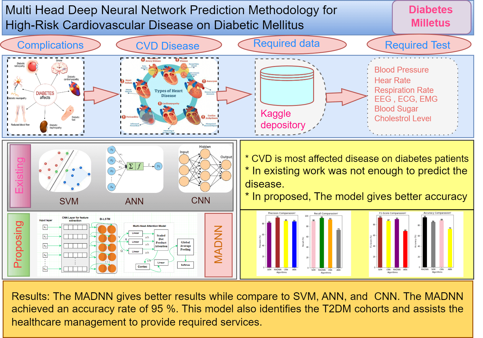
Major chronic diseases such as Cardiovascular Disease (CVD), diabetes, and cancer impose a significant burden on people and healthcare systems around the globe. Recently, Deep Learning (DL) has shown great potential for the development of intelligent mobile Health (mHealth) interventions for chronic diseases that could revolutionize the delivery of health care anytime, anywhere. The aim of this study is to present a systematic review of studies that have used DL based on mHealth data for the diagnosis, prognosis, management, and treatment of major chronic diseases and advance our understanding of the progress made in this rapidly developing field. Type 2 Diabetes Mellitus (T2DMs) is a regular chronic disorder that is caused by the secretion of insulin, which leads to serious death-related issues and the most complicated ones. Coronary Heart Disease (CHD) is the most frequent issue related to T2DM patients. The major concern is recognizing the high possibility of CHD complications, yet the model is not available to identify it. This work introduces a deep learning technique that can predict heart disease effectively using a hybrid model, which integrates DNNs (Deep Neural Networks) with a Multi-Head Attention Model called MADNN. The scheme can be designed to automatically learn the best-quality features from Electronic Health Records (EHRs), and effectively combine heterogeneous and time-sequenced medical data for predicting the risk of CVD. The analysis is done using the Kaggle dataset. The outcomes prove that the MADNN has improved accuracy by about 95% and indicates the precise accuracy is higher for the disease compared with SVM, CNN and ANN.Graphic Abstract
Keywords
Diabetes is one of the primary causes of mortality in developing nations. Nearly 1.3 billion people live in India, approximately four times the population of the United States [1,2]. 72.9 million individuals in India had DMs since 2017, up from 40.9 million in 2007. The government and the general public are investing in research to discover a cure for this viral disease. DMs are disorders where blood sugar levels consistently rise due to insulin deficiencies, which alter the blood sugar metabolism of humans. Carbohydrates that generate energy for everyday activities do not get converted into glucose sugar in diabetes in increased glucose levels and stopping bloodstreams from reaching body cells each in body cells [3].
Diabetes is a disease where blood sugar levels or blood glucose are high. It has three types: Type 1, Type 2 and Gestational diabetes. Type 1 diabetes, where the human body cannot produce enough insulin. Type 2 diabetes is a common type where the human body cannot create or utilize insulin well. Gestational diabetes will occur during pregnancy. Diabetes is the foremost cause of dangerous health problems like heart strokes, eye problems, nervous system disturbance, and kidney problems. According to survey reports in 2019, by International Diabetes Federation (IDF), the number of people who have diabetes is near to 463 million. Researchers predicted that the number of diabetes patients may increase to 642 million, i.e., one in ten adults [4]. In this circumvention, the early prediction of diabetes mellitus is important with efficient techniques to reduce the death rate. Among the diabetes cases, more people belong to Type 2 diabetes [5].
Funds have been devoted to primary research in this area, which is complex for better analysis and motivated by an emotional desire to find solutions quickly [6,7]. DMs contribute to the development of ailments including heart disease, several studies have designed predictive models for CVDs in which T2DMs were considered risk factors in the models [8]. Recently, the management dataset has found extensive application in healthcare analysis and clinical decision-making [9]. It makes longitudinal data available to understand the disease advancement and predict future effects on a particular patient [10]. Management and survey data were evaluated using risk prediction tools in 2018 trained in the detection of six chronic illnesses: congestive heart failure, DMs, obstructive pulmonary disease, lung cancer, myocardial infarction, and stroke. The potential of advanced machine learning approaches like Support Vector Machine (SVM) [11]. Random Forest (RF), and Decision Tree (DT) were examined for risk prediction and these techniques were found to be highly efficient when compared to traditional detection mechanisms [12]. The approaches showed the ability to extract meaningful patterns from considerable datasets for solving corresponding problems.
Risk predictions of CVDs in patients with T2DMs using GAs (Genetic Algorithm) and machine learning approaches [13], were introduced, and several research studies are available that exhibit differences in terms of features that are extracted, and then the classifiers were used. Due to the high data dimensionality in the data pattern, the convolutional machine learning algorithms [14] were used, but did not perform well in critical problems, for example, the detection of CVDs. The pitfalls of machine learning have inspired research in Deep Learning (DL). DL also plays a vital role in the healthcare domain. In contrast to machine learning, feature extraction, and classification are inherently carried out in deep learning networks. The hidden layers of the deep learning network perform with no external researcher being involved. Fig. 1 depicts the key contribution of the proposed model. From the research gap, this work proposes a hybrid model, which integrates DNNs with a multi-head attention model called MADNN. Initially, upgraded DNNs are built into this model for the extraction of local features related to positional invariants and by merging recurrent Bi-LSTMs (bidirectional long short-term memory) with CNNs (convolution neural networks). Subsequently, a multi-head attention model is introduced for acquiring data found in EHRs with pivotal associations, long spaces, and encoding dependencies resulting in unique highlights getting added to the outputs from Bi-LSTMs hidden layers. The scheme also avoids overfitting by using global average pooling, which converts vectors into high-level sentiment representations, and sigmoid classifiers detect CVDs.
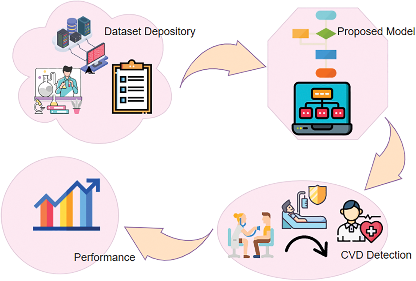
Figure 1: General framework of proposed CVD detection using MADNN
Section 1 describes the overall introduction to diabetics. Section 2 gives the analysis of various models in the literature review. Section 3 gives an overview of the proposed model. Section 4 discusses the various Experiments and results obtained. At last, Section 5 discusses the conclusion and future work.
Only a few studies that included T2DMs as risk factors have been effective in establishing prediction models for CVDs. Studied the occurrence of glucose abnormality in a sick person who contains sensitive cardiovascular syndrome and evaluated the robustness of logical and objective criteria for forecasting the pathologic results of OGTTs (oral glucose tolerance test), 3 months after the patient’s discharge. The potential study of 102 coronary care unit patients was classified using the criteria established by the American Diabetes Association. OGTTs were performed on non-diabetic individuals three months after their discharge from the unit.
In [15], the researchers used of FFRs (flow reserve fractions) to rely on deep learning for detecting the added complication of DMs. Considering the difficulties of studies on CHD with DMs and FFRs, this research concluded that contemporary coronary angiographies, which were still evolving, had promising influences on therapies offered for CHD and DMs. Based on this, the therapeutic impact of combining with FFRs could prove to be advantageous. Their study also included techniques for establishing appropriate comparison tests. In this experiment, the actual CHD along with the complications of DMs, using random classifications of every group of 41 people, was carried out, in which one group belonged to the FFRCT group, and another was from the FFRQCA group, guaranteeing the experimental impact, global evaluation indices were derived.
In [16], the researchers explored the various models which contain the SVM-based approaches to identify the sick person containing the sickness. The various types and features of the data from numerous machine learning frameworks have been figured out based on classification accuracy and efficiency. The framework was then integrated to generate a new ensemble technique by improving the efficiency and effectiveness and accuracy of the framework. The key variables have been identified from the patient data using tree-based models. The learned model helps to identify patients of different disease classes.
In [17], the authors proposed deep learning method for predicting MACE (major adverse cardiovascular events) was evaluated using data from North East Italy, 214,676 veneto patients suffering from DMs. The data included pharmacy and hospitalization claims of one year along with the patient’s basic information. This data was used to estimate 4P-MACE composite endpoints, based on cardiac-related issues which have indication horizons between 1 to 5 years. Based on the job’s time-to-event actions, the problem was cast as a multi-result.
In [18], the authors explored the relationship between HR monitors and CGMs devices for low-cost alternatives to measure glucose dysregulation. A total of 550 participants were accepted, with healthy T2DMs, pre-diabetics, and pregnant diabetic cohorts wearing CGMs and HR monitors for 10 days. Although the underlying glucose regulation and heart rates have many similarities, removing usually utilized characteristics in time series analyses provided weaker correlations among CGMs and HR data. On the other hand, by learning combined representations of CGMs and HR using CCAs (Canonical Association Analysis), CGMs and HR characteristics could be learned in CCAs space, appropriately, exhibiting statistically significant correlations. Extraction of the HR characteristics involved in the maximum of CCAs aims, in conjunction with CGMs, allows learning about patients glucose regulating systems using HR monitors, thus discarding complex CGMs.
In [19], the experts discussed two significant illnesses, diabetes, and cardiac-related approaches to anticipate hospital admissions due to these criticalities are studied. The study predicted, based on patient’s medical histories, both recent and prior times as recorded in their EHRs. Several machine learning techniques like kernelized. and sparse SVMs, sparse LRs, and RFs were used to solve it. The introduction of two innovative techniques helped in the identification of hidden patient clusters and made classifiers suitable for every cluster, balance between accuracy and comprehensibility of predictions significant to healthcare.
In [20], the authors proposed DL-based diabetes detection. In this system, Convolution Neural Network (CNN), Long Short Term Memory (LSTM), and the combined CNN-LSTM were used for detecting diabetes. Heart Rate was taken from the collected ECG signal and this model shows that diabetes can be detected through ECG signals. The maximum accuracy of 92% was achieved using CNN-LSTM with Support Vector Machine.
In [21], the researchers developed a web-based strategy to forecast diabetes using machine learning techniques on the PIMA Indian dataset. On the other hand, no single study has examined all the well-known supervised learning methods in a comprehensive manner. Srivastava et al. [22] used an ANN approach to predict diabetes using the PIMA Indian dataset. In [23], Saji et al. developed a multilayer perceptron that was used to predict diabetes. Using an auto-tuned multilayer perceptron, in [24], Jahangir et al. suggested an expert system to predict diabetes.
In [25], the experts proposed a DNN for the classification of Type 2 diabetes using stacked encoders for feature engineering, a softmax function for classification, and a backpropagation method for fine-tuning the network. Training of the model was performed with PIDD along with 786 patient records and eight features and achieved an accuracy of 86.26%.
In [26], the researchers used the decision tree technique to predict Type 2 diabetes using the PID dataset [27]. A comparison of performance using an SVM classifier showed that the decision tree successfully predicted Type 2 diabetes. In summary, the above-discussed techniques have some pros and cons, which are as follows: For example, ML algorithms such as RF, decision trees, and SVM are helpful if we use them for classification problems, except for regression, where they may not be suitable for predicting training data beyond the range. Similarly, within the decision tree, if there is a little change in data, it may affect the entire structure of the model [25].
Furthermore, SVM faces minor issues with noisy data [26]. Therefore, these ML algorithms are suitable for classification problems. However, ANN and CNN are good at making predictions because, in backpropagation, these methods obtain good results when they use gradients to update the weights. However, they have some problems, such as vanishing gradient problems or exploding gradient problems, where the value of gradients (a value used to update the weights) decreases with backpropagation, so the value becomes small and does not help much with learning. However, it is possible to overcome these limitations by applying an LSTM and GRU by using ReLU, which allows capturing the impact of the earliest given data. Moreover, by tuning the burden value during the training process, the vanishing gradient issue is usually avoided [28].
Although considerable work has been discussed regarding heart disease prediction using diabetes data, more work must be focused on. This work proposes various disease identification frameworks for CVDs in T2DMs sick people using deep learning methodologies. Its two basic goals were to (1) examine the subject’s comorbidity patterns (illness progression) from disease networks, and (2) develop prediction models to estimate the risk of CVD in patients with T2DMs based on the prior medical history of patients [29].
Initially, the proposed model initiates with CVD data as input to the CNN from the depository, then CNN generates its output to the Bi-LSTMs, after processed, its outcome was fed into a multi-head attention model and subsequently, global average pooling was utilized to get the completed representation by Soft-Max classifier, here diabetes, and mental health can be predicted using Bi-LSTMs and multi-head attention. Diabetes results in the form of high blood glucose level or low blood glucose level which is mostly considered to predict heart disease. It is achieved by one of the layers called the SoftMax layer. Fig. 2 shows the flowchart of the MADNN-based CVD detection.
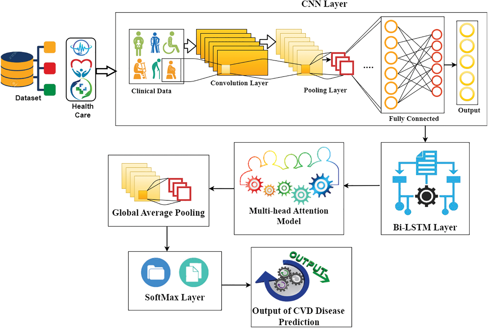
Figure 2: General framework of proposed CVD detection using MADNN
The cardiovascular disease dataset is an open-source dataset found on Kaggle (https://www.kaggle.com/datasets/sulianova/cardiovascular-disease-dataset). The data consists of 70,000 patient records (34,979 presenting with cardiovascular disease and 35,021 not presenting with cardiovascular disease) and contains 12 features as input. Some features are numerical, others are assigned categorical codes, and others are binary values. The classes are balanced, but there were more female patients observed than male patients. Furthermore, the continuous-valued features are almost normally distributed; however, most categorical-valued features are skewed towards “normal” as opposed to “high” levels of potentially pathological features. Here, the objective is not only to design a classifier to identify the presence of cardiovascular disease but also to determine which features and types of data (demographic, examination, and social history) are most useful for predicting disease. With the information gained from this study, physicians could potentially alter their current case history methods to obtain more useful data from their patients. The results from this paper could also aid in streamlining the diagnostic process and improving diagnostic accuracy.
3.2 MADNN Based CVD Detection Model
The general structure of the MADNN framework is depicted in this section, which consists of six fundamental modules known as the input layer, CNNs [30], Bi-LSTMs [31], multi-head attention model, global average pooling layer, and SoftMax layer. The MADNN model complete block diagram is seen in Fig. 2.
The MADNN models primary goal is to determine the polarity of CVDs for the given texts. The CNNs have three basic layers: convolution, pooling, and fully linked layers. Convolution layers extract the best characteristics of CVD detection. Convolution kernels are responsible for extracting certain features. The maximum counts of convolution kernels were set at 150. Convolution kernels are responsible for extracting certain features. Convolution procedures for Input Matrices IM of CNNs outputs can be written as
In Eq. (1), FM indicates the feature matrix extracted after convolution is done, and the weight matrix WM refers to the network learning parameters. To simplify the calculations, it is important to nonlinearly map the convolution output of every convolution kernel.
Eq. (2) mentioned the relu function is one among the activation functions AF that CNN models typically use. For the extensive extraction of features, in this study, convolution windows sized 2 and 3 are used for extracting the binary and ternary features belonging to the disease data. Once the convolution operation was completed, the retrieved features were sent to the pooling layer, which aggregated these features once again to simplify their expression. N-Max pooling was employed in this study as it picks the best-N maxima of the filters to reflect the information that the filters describe. The expression of the N-value is given by
In Eq. (3), where l refers to the length of input vectors [AFs] refers to the scale of the convolution window. Once the pooling function calculation is completed, the feature vector extracted by every convolution kernel is considerably reduced, and the data information associated with the core of the disease dataset is preserved because the amount of convolution kernels is fixed to 150, and the data representation matrix derived after pooling is obtained Ã
3.3 Bidirectional LSTMs (BiLSTM)
It is the extended form of conventional LSTMs, which can help in improving the model performance on sequential classification problems. The bidirectional LSTMs perform the training of two LSTMs on the input set as illustrated in Fig. 3. Due to this bidirectional behaviour, the flexibility of the input data is improved for the redundant model. Moreover, the recurrent bidirectional network improves the approachability of the various state inputs and it does not need static input data before the training process. Here, the Long Short-Term Memory (LSTMs) is used in the form of the repetitive model of the bidirectional recurrent model since it gets over the problem of vanishing/exploding gradient in the CNN. The LSTMs neural network is utilized for processing input data set with a length and attributes sequenced as [x1, x2,
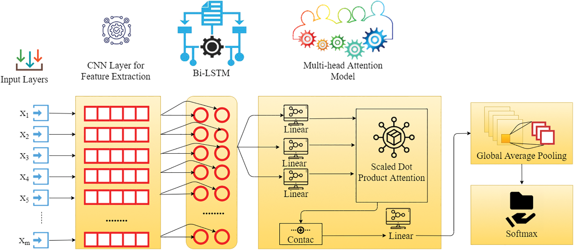
Figure 3: General framework of proposed CVD detection using MADNN
3.4 Recurrent Neural Network (RNN)
RNNs can learn sophisticated temporal dynamics through the mapping of the input set onto a set of hidden layers and their outcomes. But the diminishing and fulminate slope problem that occurs during the long-term kinetics is learned by vanilla RNNs. LSTMs resolve this by adding memory modules, letting the network go through learning to remove the earlier hidden positions, and updating them whenever there is fresh information available. The LSTMs exhibits a modern RNN framework, which can learn long distances depending upon the memory size. This framework can manage the level of information flowing from a cell. In the LSTMs model, three gates are available for the control and updating of the cell state, which is (1) Enter Data (ED inputs); (2) missed; and (3) outcome. Once the convolution operation is finished, Bi-LSTMs is used for the extraction of the features hidden in the disease data and the target too, and it is also capable of getting the long-dependent sequential information of disease data. The key concept here is to use memory cells to keep long-term past information in memory and control it using a door model. The entire process is represented in Fig. 4. There is no information provided by the door model, but it can control the amount of information. Perhaps, the addition of a gate control model is a multilevel feature selection technique. The expressions of gates and memory cells in the gate model are as follows.
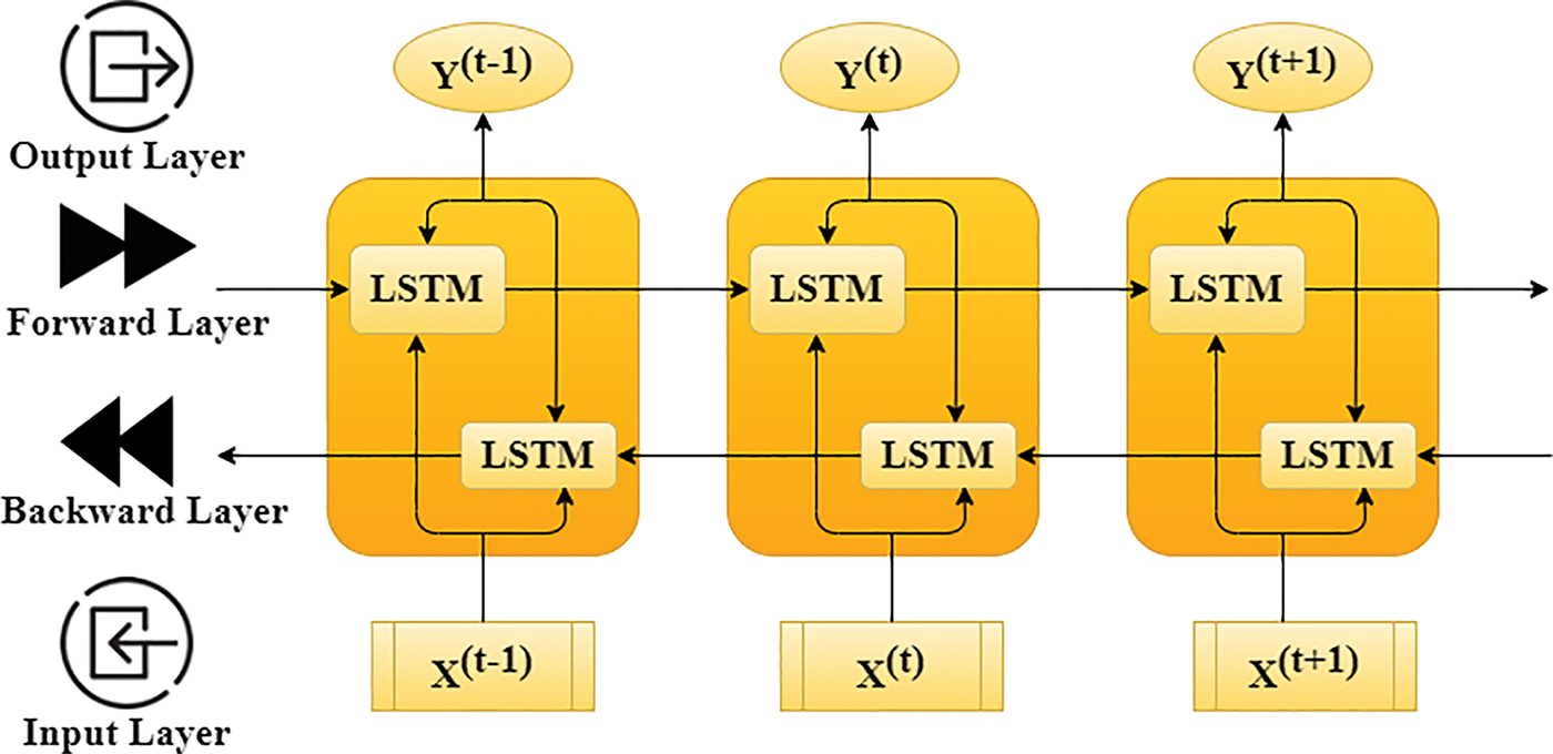
Figure 4: The architecture of three-time steps unfolding based Bi-LSTM
In the given Eq. (4), where
3.5 Multi-Head Attention Model (MA)
The observation is a primary element of the MADNN, however, a basic change exists, which involves the model capable of carrying out several distributed computations dealing with sophisticated information. A set of key pairs which are given as outcome and query mapping is what scaled dot-product attention is. To calculate the attention, four stages are used [32]. The similarity is used to calculate each key K and query weight QW. The proposed model is utilized in the event of the dot product for similarity determination. The next step to compute the attention is the scaling operation, where the factor
Fig. 5 shows the MA model block diagram. At first, QW, K, and PV are transformed linearly to produce the ED from the dot-product observation. As a result, the procedure executes computations per head at a time. As a result, it must be conducted as h, also known as multihead. For every linear transformation, Eq. (5) consists of QW, K, and PV and has various parameters. Every m-time scaled dot-product attention result is joined, and the output from the linear variation is given as the MAs outcome [33]. The formula can be expressed as shown below in Eqs. (6) and (7).
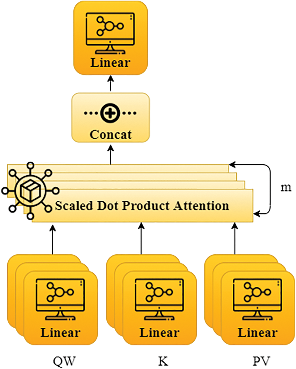
Figure 5: The block diagram of MA model
In this technique, self-attention is used to extract the inherent associations between sentences in
3.7 Global Average Pooling Layer
The completely linked system is the fundamental component of the classification system, and it includes a classification activation function and SoftMax. The overall connection of the network system stands for direction multiplication, which projects the attribute map onto a direction and then reduces its size. Entering this vector into a SoftMax layer yields the results for each stage of illness. The fully connected network is hampered by two significant disadvantages: (i) the unusually large amount of parameters reduces training duration; and, (ii) overfitting is relatively easy to achieve. Depending on the major concerns described above, global average pooling can avoid the downsides of having a similar impact, and the same order of input characteristics are included in the averaging [35–38]. In spite of giving the MA model to the disease data, The global average pooling of the input disease data is shown below in Eq. (10), here attribute array of the particular output is v, and the attribute direction of all data in the disease dataset is
Softmax Layer: For the CVD analysis prediction, the output of vector
For the assessment of the present framework, the objective of cross-entropy was introduced to show the differences between the estimated nostalgic group
Eq. (12) indicates the disease detection results. Bi-LSTMs layers can verify the context in order to prepare sequence information. MA is capable of learning details from the illustration of various directions and sizes, as well as completely extracted features, which is essential in improving the efficient enhancement of the models’ disease analysis strength directly.
4 Experimental Results and Discussion
The present work MADNN performs the classification of the gathered information into three class labels, referred to as negative or positive, and null. After the initialization of the dataset, the values will be sent through a representation function in which the data are transformed to numerical values, which uses the matrix form to be the first stage in the analysis, and next, it will be given input to the proposed model MADNN for classification of the CVD. The confusion matrix helps to determine the performance of the classifier on the basics of the test dataset. It is often used to compute performance measures such as accuracy, recall, precision, and F1-scores. The suggested techniques’ performance is compared to current approaches such as SVM [26], and CNNs [20]. In terms of the metrics obtained using the confusion matrix consisting of the corresponding equations in the above Table 1, where TP indicates True Positive yielding the overall number of disease data, which are presently CVD positive and categorized to be CVD positive. FN implies False Negative providing the overall number of disease data, which are presently CVD positive and categorized to be CVD negative. TN indicates True Negative yielding the overall number of disease data, which are presently CVD negative and categorized to be CVD negative. FP implies False Positive providing the overall number of disease data, which are presently CVD negative and categorized to be CVD positive. In the Table 1, where TP indicates True Positive yielding the overall number of disease data, which are presently CVD positive and categorized to be CVD positive. FN implies False Negative providing the overall number of disease data, which are presently CVD positive and categorized to be CVD negative.
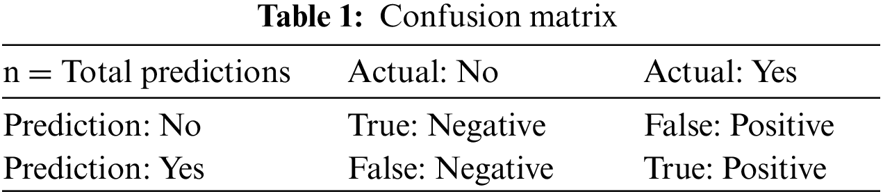
In research, the confusion matrix can be used to estimate the performance of the proposed model. It depends on the test data’s true values. The size of the matrix varies if classes vary. The matrix structure is a combination of rows and columns consist predicted values and actual values, respectively. The following Table 1 represents the sample confusion matrix where TP indicates True Positive yielding the overall number of disease data, which are presently CVD positive and categorized to be CVD positive. FN implies False Negative providing the overall number of disease data, which are presently CVD positive and categorized to be CVD negative. TN indicates True Negative yielding the overall number of disease data, which are presently CVD negative and categorized to be CVD negative. FP implies False Positive providing the overall number of disease data, which are presently CVD negative and categorized to be CVD positive. confusion matrix supports various calculations for the performance of the model such as accuracy, precision, recall, F1-score, etc.
Accuracy: It is a ratio of the total samples that were correctly classified to total number of samples as in Eq. (13).
Precision: calculates the percentage of positive class predictions that are truly positive as in Eq. (14).
Recall: calculates a single score that accounts both for precision and recall issues as in Eq. (15).
F1-score: calculates the amount of useful class predictions based on positive examples in the database as in Eq. (16).
Fig. 6 represents the result of precision. It is used to represent the quality of positive predictions. It is the combination of true and false positives in the confusion matrix. Here the percent of SVM, CNN, ANN and MADNN, and the values are 82, 85, 64 and 91, respectively. In comparison, the precision value of the proposed model gives a high rate. It also derived the factor calculation time, supporting the simple tuning of MADNN. The recall is used to identify the model based on true positive criteria. The above equations show its calculations (14), (15). Fig. 6 shows that the MADNN got a 96 percent high rate compared to other models such as SVM, CNN, and ANN, which had percentages of 90%, 93%, and 73% respectively. Increasing the number of features can maximize recall.
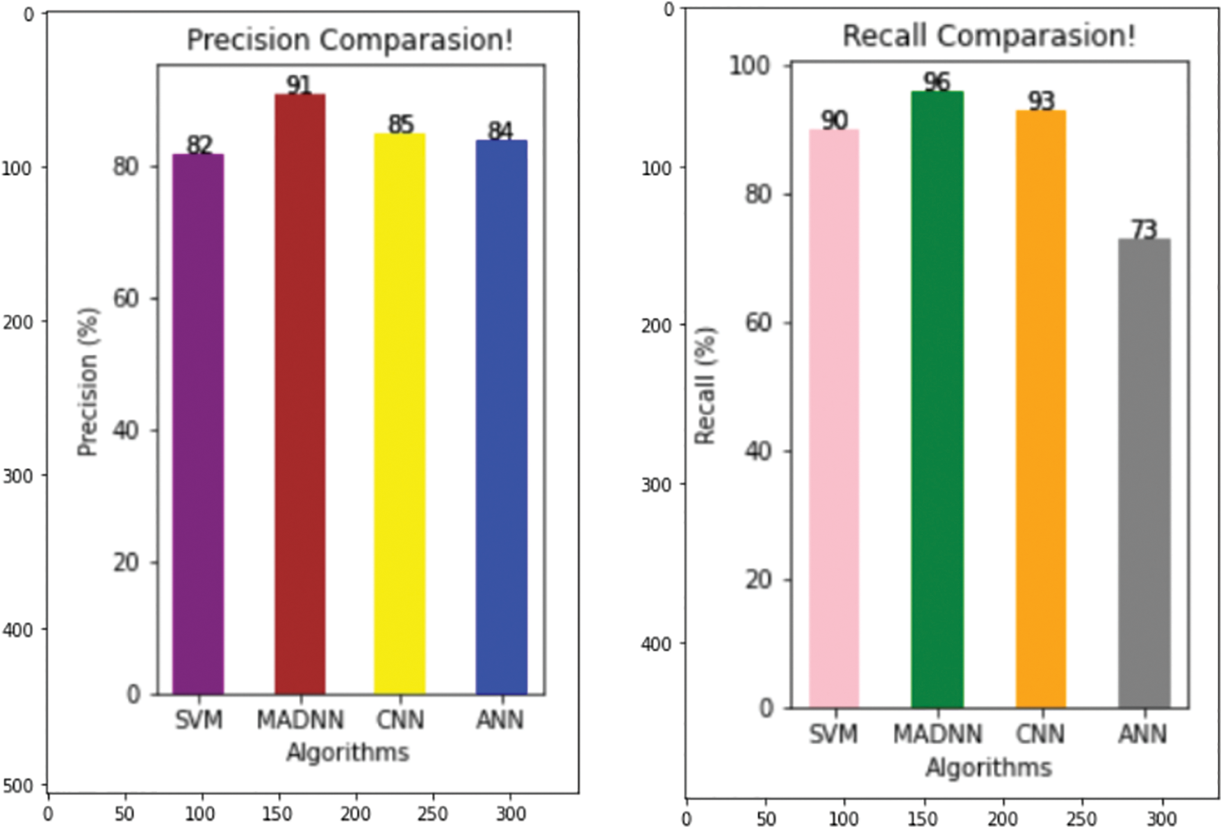
Figure 6: Comparing various models with respect to precision and recall
From Fig. 7, it is especially used when unseen occurred. It is an average of precision and recall, when the class of features is high, the f1-measure is also maximized. The F1-score of SVN, CNN, ANN, and MADNN are 90, 93, 73, and 96 percent, respectively. These enhancements were mostly due to the management of lengthy dependencies in the text utilizing bidirectional LSTMs, resulting in high F1-scores. Eqs. (13), (16) represent its calculation.
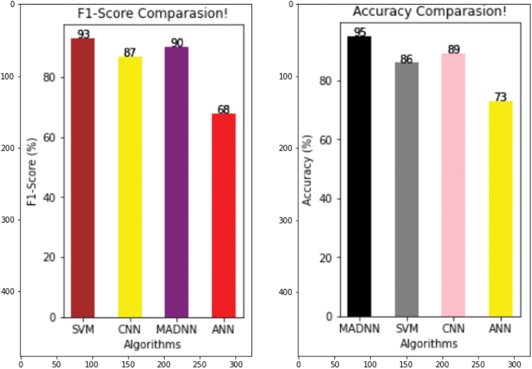
Figure 7: Comparing various models with respect to F1-score and accuracy
From Fig. 7, in ML/DL, the quality of the models is estimated by their accuracy. It is calculated by considering the correct prediction over the test data. Fig. 7 shows the high accuracy compared to existing models. The accuracy percent of SVM, CNN, ANN, and MADNN are 86, 89, 73, and 95, respectively. Thus, the suggested approach outcomes the current technique in finding the predicted CVD in terms of good validation.
In this paper, we proposed a novel hybrid deep neural network technique to improve the accuracy of CVD prediction with the EHR. Data pre-processing for the CVD is done with the help of a python tool. The outcomes of the proposed model are compared with the machine learning methods, where the deep learning technique obtained a higher accuracy value in predicting the risk of the disease. The MADNN gives better results compared to SVM, ANN, and CNN. The MADNN achieved an accuracy rate of 95%. This model also identifies the T2DM cohorts and assists the healthcare management to provide better services. However, the MADNN cannot give efficient results for fewer datasets, which can be resolved in the future. The work can be extended and improved for automated diabetes analysis by including some other deep-learning algorithms and techniques. The amount of data that the model can handle is high. In the hyperparameter tuning method, because training too many parameters can easily result in overfitting, the algorithm can also simply modify the last output layer. If the data are too different from the original dataset, the model can tune half of the layer after fine-tuning the output of the top layer.
Funding Statement: The authors received no specific funding for this study.
Conflicts of Interest: The authors declare that they have no conflicts of interest to report regarding the present study.
References
1. Ranasinghe, P., Jayawardena, R., Gamage, N., Sivanandam, N., Misra, A. (2021). Prevalence and trends of the diabetes epidemic in urban and rural India: A pooled systematic review and meta-analysis of 1.7 million adults. Annals of Epidemiology, 58(6), 128–148. https://doi.org/10.1016/j.annepidem.2021.02.016 [Google Scholar] [PubMed] [CrossRef]
2. Sukkarieh-Haraty, O., Egede, L. E., Khazen, G., Abi Kharma, J., Farran, N. et al. (2022). Results from the first culturally tailored, multidisciplinary diabetes education in Lebanese adults with Type 2 diabetes: Effects on self-care and metabolic outcomes. BMC Research Notes, 15(1), 39. https://doi.org/10.1186/s13104-022-05937-0 [Google Scholar] [PubMed] [CrossRef]
3. Yazdani, N. M., Moghaddam, R. K. (2021). Blood glucose regulation in patients with Type 1 diabetes by robust optimal safety critical control. Frontiers in Health Informatics, 10(1), 80. https://doi.org/10.30699/fhi.v10i1.286 [Google Scholar] [CrossRef]
4. Singh, A., Halgamuge, M. N., Lakshmiganthan, R. (2017). Impact of different data types on classifier performance of random forest, naive bayes, and k-Nearest Neighbors algorithms. International Journal of Advanced Computer Science and Applications, 8(12). [Google Scholar]
5. Varma, R., Bressler, N. M., Doan, Q. V., Gleeson, M., Danese, M. et al. (2014). Prevalence of and risk factors for diabetic macular edema in the United States. JAMA Ophthalmology, 132(11), 1334–1340. https://doi.org/10.1001/jamaophthalmol.2014.2854 [Google Scholar] [PubMed] [CrossRef]
6. Sneha, N., Gangil, T. (2019). Analysis of diabetes mellitus for early prediction using optimal features selection. Journal of Big Data, 6(1), 1–19. https://doi.org/10.1186/s40537-019-0175-6 [Google Scholar] [CrossRef]
7. Rajbhandari, J., Fernandez, C. J., Agarwal, M., Yeap, B. X. Y., Pappachan, J. M. (2021). Diabetic heart disease: A clinical update. World Journal of Diabetes, 12(4), 383–406. https://doi.org/10.4239/wjd.v12.i4.383 [Google Scholar] [PubMed] [CrossRef]
8. Nathanson, D., Sabale, U., Eriksson, J. W., Nyström, T., Norhammar, A. et al. (2018). Healthcare cost development in a Type 2 diabetes patient population on glucose-lowering drug treatment: A nationwide observational study 2006–2014. PharmacoEconomics-Open, 2(4), 393–402. https://doi.org/10.1007/s41669-017-0063-y [Google Scholar] [PubMed] [CrossRef]
9. Tokajian, S., Merhi, G., Al Khoury, C., Nemer, G. (2022). Interleukin-37: A link between COVID-19, diabetes, and the black fungus. Frontiers in Microbiology, 12, 788741. https://doi.org/10.3389/fmicb.2021.788741 [Google Scholar] [PubMed] [CrossRef]
10. Reddy, G. T., Reddy, M. P. K., Lakshmanna, K., Rajput, D. S., Kaluri, R. et al. (2020). Hybrid genetic algorithm and a fuzzy logic classifier for heart disease diagnosis. Evolutionary Intelligence, 13(2), 185–196. https://doi.org/10.1007/s12065-019-00327-1 [Google Scholar] [CrossRef]
11. Ng, R., Sutradhar, R., Wodchis, W. P., Rosella, L. C. (2018). Chronic disease population risk tool (CDPoRTA study protocol for a prediction model that assesses population-based chronic disease incidence. Diagnostic and Prognostic Research, 2(1), 1–11. https://doi.org/10.1186/s41512-018-0042-5 [Google Scholar] [PubMed] [CrossRef]
12. Preethi, I., Dharmarajan, K. (2020). Diagnosis of chronic disease in a predictive model using machine learning algorithm. 2020 International Conference on Smart Technologies in Computing, Electrical and Electronics (ICSTCEE), pp. 191–196. IEEE. [Google Scholar]
13. Patil, P. B., Shastry, P. M., Ashokumar, P. (2020). Machine learning based algorithm for risk prediction of cardio vascular disease (CVD). Journal of Critical Reviews, 7(9), 836–844. [Google Scholar]
14. Wang, Z., Yin, H., Jing, W., Sun, H., Ru, M. et al. (2022). Application of CT coronary flow reserve fraction based on deep learning in coronary artery diagnosis of coronary heart disease complicated with diabetes mellitus. Neural Computing and Applications, 34(9), 6763–6772. https://doi.org/10.1007/s00521-021-06070-y [Google Scholar] [CrossRef]
15. Dinh, A., Miertschin, S., Young, A., Mohanty, S. D. (2019). A data-driven approach to predicting diabetes and cardiovascular disease with machine learning. BMC Medical Informatics and Decision Making, 19(1), 1–15. https://doi.org/10.1186/s12911-019-0918-5 [Google Scholar] [PubMed] [CrossRef]
16. Gundluru, N., Rajput, D. S., Lakshmanna, K., Kaluri, R., Shorfuzzaman, M. et al. (2022). Enhancement of detection of diabetic retinopathy using harris hawks optimization with deep learning model. Computational Intelligence and Neuroscience, 2022(24), 1–13. https://doi.org/10.1155/2022/8512469 [Google Scholar] [PubMed] [CrossRef]
17. Rashtian, H., Torbaghan, S. S., Rahili, S., Snyder, M., Aghaeepour, N. (2021). Heart rate and cgm feature representation diabetes detection from heart rate: Learning joint features of heart rate and continuous glucose monitors yields better representations. IEEE Access, 9, 83234–83240. https://doi.org/10.1109/ACCESS.2021.3085544 [Google Scholar] [CrossRef]
18. Brisimi, T. S., Xu, T., Wang, T., Dai, W., Adams, W. G. et al. (2018). Predicting chronic disease hospitalizations from electronic health records: An interpretable classification approach. Proceedings of the IEEE, 106(4), 690–707. https://doi.org/10.1109/JPROC.2017.2789319 [Google Scholar] [PubMed] [CrossRef]
19. Shetty, B., Fernandes, R., Rodrigues, A. P., Chengoden, R., Bhattacharya, S. et al. (2022). Skin lesion classification of dermoscopic images using machine learning and convolutional neural network. Scientific Reports, 12(1), 18134. https://doi.org/10.1038/s41598-022-22644-9 [Google Scholar] [PubMed] [CrossRef]
20. Swapna, G., Kp, S., Vinayakumar, R. (2018). Automated detection of diabetes using cnn and CNN-LSTM network and heart rate signals. Procedia Computer Science, 132(4), 1253–1262. https://doi.org/10.1016/j.procs.2018.05.041 [Google Scholar] [CrossRef]
21. Zou, Q., Qu, K., Luo, Y., Yin, D., Ju, Y. et al. (2018). Predicting diabetes mellitus with machine learning techniques. Frontiers in Genetics, 9, 515. https://doi.org/10.3389/fgene.2018.00515 [Google Scholar] [PubMed] [CrossRef]
22. Srivastava, S., Sharma, L., Sharma, V., Kumar, A., Darbari, H. (2019). Prediction of diabetes using artificial neural network approach. In: Engineering vibration, communication and information processing, pp. 679–687. India, Springer. [Google Scholar]
23. Saji, S. A., Balachandran, K. (2015). Performance analysis of training algorithms of multilayer perceptrons in diabetes prediction. 2015 International Conference on Advances in Computer Engineering and Applications, pp. 201–206. IEEE. [Google Scholar]
24. Jahangir, M., Afzal, H., Ahmed, M., Khurshid, K., Nawaz, R. (2017). An expert system for diabetes prediction using auto tuned multi-layer perceptron. 2017 Intelligent Systems Conference (IntelliSys), pp. 722–728. IEEE. [Google Scholar]
25. Kannadasan, K., Edla, D. R., Kuppili, V. (2019). Type 2 diabetes data classification using stacked autoencoders in deep neural networks. Clinical Epidemiology and Global Health, 7(4), 530–535. https://doi.org/10.1016/j.cegh.2018.12.004 [Google Scholar] [CrossRef]
26. Apoorva, S., Aditya, S. K., Snigdha, P., Darshini, P., Sanjay, H. (2020). Prediction of diabetes mellitusType 2 using machine learning. In: Computational vision and bio-inspired computing: ICCVBIC 2019, pp. 364–370. Springer. [Google Scholar]
27. Kamble, A. K., Manza, R. R., Rajput, Y. M. (2016). Review on diagnosis of diabetes in Pima Indians. International Journal of Computers and Applications, 975, 8887. [Google Scholar]
28. Yamashita, R., Nishio, M., Do, R. K. G., Togashi, K. (2018). Convolutional neural networks: An overview and application in radiology. Insights into Imaging, 9(4), 611–629. https://doi.org/10.1007/s13244-018-0639-9 [Google Scholar] [PubMed] [CrossRef]
29. Enrico, L., Fadini, G. P., Sparacino, G., Avogaro, A., Tramontan, L. et al. (2021). A deep learning approach to predict diabetes’ cardiovascular complications from administrative claims. IEEE Journal of Biomedical and Health Informatics, 25(9), 3608–3617. https://doi.org/10.1109/JBHI.2021.3065756 [Google Scholar] [PubMed] [CrossRef]
30. Kingma, F., Abbeel, P., Ho, J. (2019). Bit-Swap: Recursive bits-back coding for lossless compression with hierarchical latent variables. International Conference on Machine Learning, pp. 3408–3417. PMLR. [Google Scholar]
31. Graves, A., Jaitly, N., Mohamed, A. R (2013). Hybrid speech recognition with deep bidirectional LSTM. 2013 IEEE Workshop on Automatic Speech Recognition and Understanding, pp. 273–278. IEEE. [Google Scholar]
32. Manjulatha, B., Pabboju, S. (2021). An ensemble model for predicting chronic diseases using machine learning algorithms. In: Smart computing techniques and applications, vol. 2, pp. 337–345. Springer. [Google Scholar]
33. Wan, X. (2009). Co-training for cross-lingual sentiment classification. Proceedings of the Joint Conference of the 47th Annual Meeting of the ACL and the 4th International Joint Conference on Natural Language Processing of the AFNLP, pp. 235–243. [Google Scholar]
34. Sutskever, I., Vinyals, O., Le, Q. V. (2014). Sequence to sequence learning with neural networks. In: Advances in neural information processing systems, vol. 27. [Google Scholar]
35. Longato, E., di Camillo, B., Sparacino, G., Saccavini, C., Avogaro, A. et al. (2020). Diabetes diagnosis from administrative claims and estimation of the true prevalence of diabetes among 4.2 million individuals of the Veneto region (North East Italy). Nutrition, Metabolism and Cardiovascular Diseases, 30(1), 84–91. https://doi.org/10.1016/j.numecd.2019.08.017 [Google Scholar] [PubMed] [CrossRef]
36. Lefebvre, P. (2005). Diabetes yesterday, today and tomorrow. the action of the international diabetes federation. Revue Medicale de Liege, 60(5–6), 273–277. [Google Scholar] [PubMed]
37. Hossain, M. E., Uddin, S., Khan, A., Moni, M. A. (2020). A framework to understand the progression of cardiovascular disease for Type 2 diabetes mellitus patients using a network approach. International Journal of Environmental Research and Public Health, 17(2), 596. https://doi.org/10.3390/ijerph17020596 [Google Scholar] [PubMed] [CrossRef]
38. Rajput, D. S., Basha, S. M., Xin, Q., Gadekallu, T. R., Kaluri, R. et al. (2022). Providing diagnosis on diabetes using cloud computing environment to the people living in rural areas of India. Journal of Ambient Intelligence and Humanized Computing, 13, 2829–2840. https://doi.org/10.1007/s12652-021-03154-4 [Google Scholar] [CrossRef]
Cite This Article
 Copyright © 2023 The Author(s). Published by Tech Science Press.
This work is licensed under a Creative Commons Attribution 4.0 International License , which permits unrestricted use, distribution, and reproduction in any medium, provided the original work is properly cited.
 Downloads
 Citation Tools