A Time-Varying Parameter Estimation Method for Physiological Models Based on Physical Information Neural Networks

1  Introduction

Differential equations describing dynamical processes are widely utilized in physics [1], engineering [2], medicine [3], biology [4], physiology, and other fields. In the practical application of differential equations, it may also involve the solution of the inverse problem, that is, when the boundary conditions and some parameters in the equation are unknown, accurate model parameters can be obtained through some measured data. Physiological processes are often described by differential equations [5]. For example, the reactions of enzymes and transporters are described by metabolic equations to reveal the mechanism leading to diabetes [6]; the process of drug concentration changes in body compartments is studied by uncertainty differential equations [7]; and the kinetic characteristics between membrane voltage and ion channels are described by electrophysiological equations, namely the Hodgkin-Huxley (HH) equation [8]. Such equations can not only be employed to describe the electrical activity of neurons, but also guide the construction of the artificial neural network [9]. The most critical and basic step in establishing the equation is the determination of time-varying parameters, such as the switch rate parameters and conductivity of ion channels. In general, all these parameters are determined by experimental measurements, usually obtained by voltage clamp or patch clamp experiments, which work with complicated steps, high difficulty, and high experimental skills [10]. Obviously, these facts motivate us to search for faster ways to estimate the time-varying parameters of electrophysiological equations, except that this presents the same challenges of time-varying parameter prediction as other differential equations [11].

In recent years, Physics-Informed Neural Networks (PINN) have achieved good performance in solving complex differential equations [12–17], becoming an alternative simple method for tackling many problems in computational science and engineering. In particular, PINN can efficiently address the forward and inverse problems of nonlinear ordinary differential equations without the need for grids in finite difference methods. Since conventional neural network models require labeled or large amounts of data, it is difficult to solve the inverse problem using this method. In addition, PINN is different from algorithms such as BP neural network [18] and semi-supervised learning [19,20] which are considered “black boxes”. PINN can integrate all given information (such as electrophysiological equations, experimental data, and initial conditions) into the loss function of the neural network, thereby recasting the original problem into an equivalent optimization problem.

How to predict time-varying parameters in differential equations is a problem we need to handle at present. However, traditional parametric prediction methods are usually based on linear and non-time-varying premises, which is not easy to achieve for the time-varying parameter determination of general nonlinear systems. Although PINN allows us to obtain time-varying parameters, conventional PINN is slow to converge in dealing with inverse problems of complex differential equations. In addition, the values of membrane potential and switch rate in HH are not in the order of magnitude, requiring a long training time. In summary, existing PINN cannot predict the time-varying parameters of HH accurately. For this purpose, this paper proposes a novel time-varying parameter estimation framework for electrophysiological models based on physical information neural networks, named BioE-PINN. This framework offers a total loss function based on the Hodgkin-Huxley equation, observed data errors, and hard constraints on initial conditions. The training time can be reduced, and the prediction accuracy can be improved of the model after modifying the ion channel switch rate equation. Furthermore, the stimulation currents that evoke membrane potentials can be predicted.

The contributions of this paper are summarized as follows:

1. We propose a new PINN-based framework for time-varying parameter estimation in electrophysiological differential equations that combines physical prior knowledge of bioelectrodynamics with advanced deep learning. The loss function of a neural network is carefully designed to not only perfectly predict observations (i.e., data-driven losses), but also take into account the underlying physics (i.e., physics-based losses).

2. We employ hard constraints to accommodate differences between orders of magnitude and adaptive activation functions to accelerate the convergence of BioE-PINN.

3. We verify the effectiveness of the model with simulation experiments and real experimental data, using membrane potential to predict the conductivity and switch rate parameters of ion channels and pumps of electrophysiological equations.

The rest of this paper is organized as follows. Section 2 reviews the related work of PINN in solving the inverse problem. Section 3 discusses in depth the details of our proposed method. Section 4 presents the experiments and results. Section 5 shows the conclusion and outlook.

2  Related Work

Parameter inference from observational data is a core problem in many fields and quite an important research direction in process modeling. Traditional parameter prediction methods are usually based on linearity and time-invariance, but the parameter determination of general nonlinear systems is not easy to achieve. The neural network has the advantages of strong approximation ability, a high degree of nonlinearity, strong self-learning, and self-adaptation, and has been widely exploited in the parameter determination of nonlinear systems.

In recent years, with the further development of deep learning and computing resources, a deep learning algorithm framework called Physics-informed Neural Network has been proposed [21]. It mainly employs automatic differentiation techniques to solve forward and inverse problems of ordinary differential equations. PINN can be trained with a small amount of data and has better generalization performance while maintaining accuracy [21]. With the emergence of PINN, a lot of follow-up research work is triggered. Some of the research focuses on improving the accuracy and efficiency of PINN, and then adaptive activation functions can be applied to improve the performance of PINN in solving differential equations. This method introduces a scaling factor and a learnable parameter into the activation function of the neural network, and the factor and the parameters of the neural network are updated synchronously during training [22]. Residual points in PINN are usually randomly distributed among grid points on the domain, which may result in a large amount of data required to train the model. To address this problem, gPINNs embed the gradient information of the physical equations into the loss of the neural network to achieve better accuracy while using fewer data [23].

In PINN, multiple loss terms appear corresponding to the residuals, initial values, and boundary conditions of the equation, and it is critical to balance these different loss terms. By reviewing the latest literature, we found that the imbalance of loss functions in PINNs can be addressed by employing meta-learning techniques. And it can be applied to discontinuous function approximation problems with different frequencies, advection equations with different initial conditions and discontinuous solutions [24].

In addition, researchers have developed a large number of software libraries designed for PINNs, most of which is based on Python, such as DeepXDE [25], SimNet [26], NeuroDiffEq [27], SciANN [28], etc. The development of the software library facilitates the popularization and application of PINN. We will introduce the application of PINN in parameter prediction below.

The A-PINN framework uses a multi-output neural network to simultaneously represent the main variables and equation integrals in nonlinear integrodifferential equations, solving integral discdiscretization and truncation errors. Since A-PINN does not set fixed grids and nodes, unknown parameters can be discovered without interpolation [29]. Inferring compressibility and stiffness parameters from a material’s ultrasonic data encounters an ill-posed inverse problem. Shukla et al. implement the in-plane and out-of-plane elastic wave equations by using two neural networks in PINN and employing adaptive activation functions to accelerate their convergence [30]. Another advantage of PINN is to accelerate industrial production processes. For example, FlowDNN is 14,000 times faster than traditional methods in computational fluid dynamics simulation. It directly predicts flow fields by giving fluid constraints and initial shapes, and utilizes graphics processing units to speed up the training process of neural networks [31]. XPINNs solve the ill-posed inverse problems in designing dedicated high-speed aircraft, and the model is able to predict parameters such as air density, pressure, and so on, based on observations. The main advantage of XPINNs is the decomposition of the spatiotemporal domain, which introduces a generalization trade-off. It decomposes complex solutions of differential equations into simple parts, thereby reducing the complexity required for network learning in various subdomains and improving generalization. Compared to traditional methods, this decomposition results in less training data available in each subdomain and less time required for training [32].

PINN also has applications in the parameter determination of electrophysiological equations. For example, to capture multi-channel data related to cardiac electrical activity from high-dimensional body sensor data, a modified P-DL framework based on PINN is proposed. The framework adds a balancing metric to optimize the model training process. P-DL assists medical scientists in monitoring and detecting abnormal cardiac conditions, handling the inverse ECG modeling problem, that is, predicting spatiotemporal electrodynamics in the heart from electrical potential [33]. To aid in the treatment and diagnosis of cardiac arrhythmias, Herrero Martin et al. proposed a tool called EP-PINNs, which applies PINN to cardiac action potential simulations. The tool can predict precise action potential and duration parameters using sparse action potential data [34]. EP-PINNs are based on the Aliev-Panfilov electrophysiological model, which has the advantage of modeling action potentials without considering ion channels. However, ion channels play an important role in life activities. For example, calcium ion channels have an effect on human blood pressure, and doctors use calcium ion channel blockers as the first choice for antihypertensive drugs [35]. Therefore, predicting the kinetic parameters of ion channels and pumps is a problem that needs to be solved.

The above studies show that PINN has been continuously improved since its original proposal and has been applied to differential equation solving and predicting constant parameters. The above also provides a feasible indication for applying PINN to the time-varying parameter estimation method of physiological models in this study.

3  Methodology

In this section, we propose a physics-based neural network to estimate parameters in electrophysiological equations. Compared with traditional PINN, our proposed BioE-PINN contains hard constraints and an adaptive activation function method, which can improve the accuracy of PINN.

3.1 Physiological Equations of Cell Membrane Potential

The core mathematical framework for current biophysical-based neural modeling was developed by Hodgkin and Huxley. It is one of the most successful mathematical models of complex biological processes that have been proposed so far [36]. The cell membrane potential equations proposed in this paper are improved on the basis of the Hodgkin-Huxley (HH) equation, which can be applied to plant electrical signal modeling:

CdVdt=I(t)−g¯L(V−EL)−∑i=1ng¯imk1hk2nk3(V−Ei),t0≤t≤tfinal,(1)

dndt=αn(V)(1−n)−βn(V)n,(2)

dmdt=αm(V)(1−m)−βm(V)m,(3)

dhdt=αh(V)(1−h)−βh(V)h,(4)

V(t0)=V0,n(t0)=n0,m(t0)=m0,h(t0)=h0.(5)

where V represents the membrane potential. i represents the ion index, such as sodium, potassium, calcium, hydrogen, and chloride ions. t represents time, and the initial and final times are denoted as t0 and tfinal, respectively. I(t) is the input current stimulus. C=1μF/cm2 is the capacity of the cell membrane. g¯i and g¯L represent the maximum conductance of the ion channel and leakage current, respectively. Ei and EL represent the reverse potentials of the ion channel and leakage current, respectively. n, m, h are gating variables, their values are between 0 and 1. Each gating variable satisfies a differential equation, such as Eqs. (2)–(4). k1,2,3 are the gating variable coefficients, and their values are related to the species with 0–5. α(V) and β(V) are the voltage-dependent rate constants corresponding to the gate going from closed to open and from open to closed, respectively. We refer to [37] to modify the equations of α(V) and β(V) as Eqs. (6) and (7). V0 represents the initial membrane potential value. n0, m0, as well as h0 represent the initial gating variable values, respectively.

αi(V)=AαiV+Bαi,i=(n,m,h).(6)

βi(V)=AβiV+Bβi,i=(n,m,h).(7)

where Aαi, Bαi, Aβi and Bβi are the switch rate parameters of the voltage-dependent ion channel.

3.2 BioE-PINN Approach

When using PINN to predict the switch rate, it is first necessary to construct a feedforward neural network to approximate the electrical signal or rate. A feedforward neural network consists of an input layer, multiple hidden layers, and an output layer. Information is passed layer by layer in one direction. The value of any neuron in the network is calculated by the sum of the products of the weights and outputs of the previous layer, and then activated by a specific activation function. The relationship between two adjacent layers is usually described by the following equation:

an=σ(bn+Wnan−1),1<n≤K.(8)

where σ(⋅) represents the activation function. K is the total number of layers. bn and Wn represent the weight matrix and bias vector of layer-(n), respectively. an and an−1 represent the n and n−1 layers of the neural network, respectively.

This paper aims to solve the inverse problem of membrane potential V(t,n,m,h) through Deep Neural Network (DNN) modeling. Here, we implement a basic neural network structure using a custom loss function constrained by the laws of physics (see Eqs. (1)–(4)) to deal with the inverse problem while being able to predict the electrical signals produced by different stimulation currents. The detailed construction of BioE-PINN is presented below.

Fig. 1 demonstrates the proposed BioE-PINN. The solution to the inverse problem is parameterized by a trained DNN that satisfies not only the laws of physics but also data-driven constraints on membrane potential. Specifically, we estimate the time map of membrane potential as:

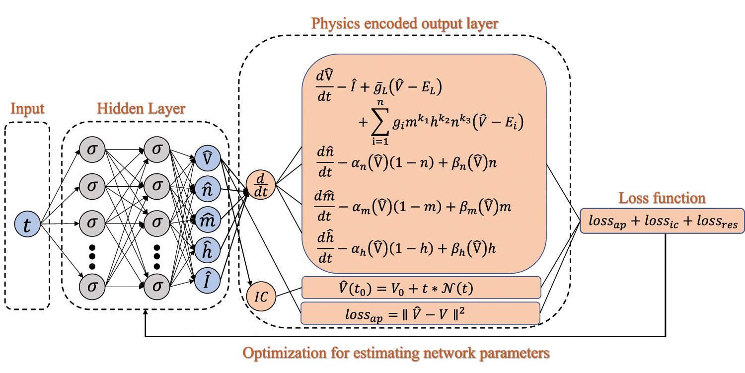
Figure 1: Schematic of the BioE-PINN for switch rates prediction

[t]⟹𝒩(t;θNN)[V(t),n(t),m(t),h(t)].(9)

where 𝒩(t;θNN) defines the DNN model. t represents the time coordinate. θNN represents the parameters to be optimized of the DNN. In particular, the input of DNN, i.e., 𝒩(t;θNN) consists of time coordinates [t], its hidden layer approximates complex functional relationships, and its output layer estimates V^(t,θNN),m^(t,θNN),h^(t,θNN) and n^(t,θNN) and I^(t,θNN). We further encode the laws of physics into the DNN by defining a unique weighted loss function:

ℒ(θNN)=ωapℒap+ωphℒph+ℒic.(10)

where the weights of data-driven loss and physics-based loss are rescaled by ωap and ωph, because data-driven loss and physics-based loss may be orders of magnitude imbalanced with each other and hinder model training.

The data-driven loss function is designed to solve the inverse problem. In order to infer the parameters in the differential equation based on the membrane potential, the predicted value of the neural network needs to be close to the real membrane potential. We define the data-driven loss:

ℒap=1Nap∑Nap((V^(t)−V(t))2).(11)

where Nap represents the size of the dataset used for model training. The residual based on the electrophysiological model is defined as:

rV(t;θNN):=CdVdt−I(t)+g¯imk1hk2nk3(V−Ei)+g¯L(V−EL),rn(t;θNN):=dndt−αn(V)(1−n)+βn(V)n,rm(t;θNN):=dmdt−αm(V)(1−m)+βm(V)m,rh(t;θNN):=dhdt−αh(V)(1−h)+βh(V)h.(12)

Physiologically based constraints will be implemented by minimizing the magnitudes of rV(t;θNN), rn(t;θNN), rm(t;θNN) and rh(t;θNN). Therefore, the loss based on the electrophysiological model is defined as:

ℒph=1Nph∑i=1Nph((rV(t;θNN))2+(rn(t;θNN))2+(rm(t;θNN))2+(rh(t;θNN))2).(13)

where Nph represents the total number of selected time points. The loss based on the electrophysiological model, i.e., ℒph, is encoded as a DNN loss function to comply with fundamental physical laws in membrane potential modeling.

To calculate the loss function during DNN training, it is necessary to obtain the derivatives of V(t),n(t),m(t),h(t) with respect to time variables. This can be easily achieved by automatic differentiation, which is free from truncation and round-off errors compared to traditional numerical differentiation [32]. Automatic differentiation is a method to differentital. Derivatives are calculated by decomposing the differential of multiple paths using the chain rule. In this study, automatic differentiation is exploited to obtain derivatives with respect to the time coordinate t in order to encode the laws of physics into DNNs in the form of ordinary differential equations.

When conventional PINN solves time-dependent ordinary differential equations or inversion of parameters, the constraints of initial conditions are mainly in the form of soft constraints, which will affect the calculation accuracy to a certain extent [38]. To this end, we propose hard constraints so that the output of the network automatically satisfies the initial conditions. Specifically, we define the residuals of the initial conditions as:

ric(t;θNN):=V^(t,θNN)−V0+t0∗𝒩(t).(14)

Hard constraints based on initial conditions will be achieved by minimizing the size of ric(t;θNN). Therefore, the loss based on the initial conditions is defined as:

ℒic=1Nic∑i=1Nic(ric(t;θNN))2.(15)

3.3 Adaptive Activation Functions

Regarding the activation functions in neurons, there are currently Sigmoid, Logistic, tanh, sin, cos, and so on, as well as ReLU, and various variants based on ReLU, ELU, Leakly ReLU, PReLU, and so forth. The purpose of introducing the activation function is to make the neural network have the characteristics of expressing nonlinearity. The activation function plays an important role in the training process of the neural network, because the calculation of the gradient value of the loss function depends on the optimization of the network parameters, and the optimization learning of the network parameters depends on the derivability of the activation function.

The size of a neural network is related to its ability to express the complexity of a problem. Complex problems require a deep network, which is difficult to train. In most cases, choosing an appropriate architecture based on the experience of the rest of the scholars requires a large number of experimental approaches. This paper considers tuning the network structure for optimal performance. To this end, a learnable parameter a=a1,…,anunit is introduced into the activation function, where nunit represents the number of neurons in each hidden layer. The activation function looks like this:

fact(a(Wx+b)).(16)

The learnable parameter a is set as a parameter in the network for optimization learning. The resulting optimization problem finds the minimum value of the loss function by updating the network parameter a, weight W and bias b, which can be expressed as:

a∗=arg⁡mina∈R+{0}(J(a)).(17)

The learnable parameter a can change the slope of the activation function. The corresponding expressions for these activation functions are given by:

Sigmoid:11+e−ax.(18)

tanh:eax−e−axeax+e−ax.(19)

ReLU:max(0,ax).(20)

The learning rate has a dramatic impact when searching for a global minimum. Larger learning rates may skip the global minimum, while smaller learning rates increase computational cost. In the training process of PINN, a small learning rate is generally used, which makes the convergence slow. In order to speed up the convergence, a scaling factor n>1 multiplied by a is introduced to speed up the convergence to the global minimum. The final expression of the adaptive activation function is given by:

fact(na(Wx+b)).(21)

3.4 Complexity Analysis

After establishing the PINN network for estimating the time-varying parameters of the electrophysiological equation, combined with the improved adaptive activation function algorithm in this paper, the prediction of the switching rate parameters in the electrophysiological equation can be realized. The algorithm is summarized as follows:

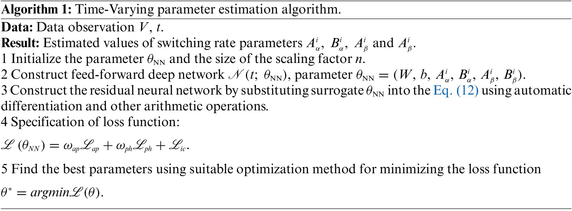
The main factors affecting the time complexity of the BioE-PINN algorithm are the number of iterations n, the number of training samples t in the neural network, and the number of hidden layer nodes. Specifically, the time complexity of creating learnable parameters in Step 2 of Algorithm 1 is O(1); Step 3 is to build a residual neural network, and its time complexity is O(1); the complexity of calculating the loss function in Step 4 is O(1+1+1); Step 5 is to train the neural network, and its purpose is to minimize the loss function. We used the FLoating-point Operations metric [39,40] to measure the time complexity of the model. A 3-layer neural network is used in BioE-PINN, which has i, j and k nodes, respectively, and its complexity is O(nt∗(ij+jk)). So the time complexity of BioE-PINN is O(BioE−PINN)=n∗(O(1)+O(1)+O(3)+O(t∗(ij+jk)))≈O(nt∗(ij+jk)), the average time complexity is O(n), and the minimum time complexity is O(n).

3.5 Evaluation Indicators

In order to evaluate the error of predicted and observed values, the following indicators are exploited: Spearman correlation coefficient (SPCC) and Root Mean Square Error (RMSE). In addition, Relative Errors are employed to evaluate the effect of parameter prediction.

SPCC=1−6∑i=1ndi2(n3−n).(22)

RMSE=1n∑i=1n(xi−xl^)2.(23)

 Relative Errors =|y−y^y|100%.(24)

SPCC is used to measure the correlation between two variables, especially shape similarity. RMSE reflects the degree of difference between the predicted value and the real value, and a smaller RMSE means that the accuracy of the predicted value is higher.

4  Results and Discussion

In this section, we first use conventional PINN and BioE-PINN to predict the parameters of HH. Specifically, we obtain the observation data through simulation, determine the HH parameters according to the observation data and compare them with the real parameters. Subsequently, we conduct experiments on the inference of electrophysiological equation parameters in animals as well as plants, and solve the HH equation according to the parameters determined by BioE-PINN. To demonstrate the effectiveness of the proposed method, various comparisons are performed. In this study, we implement BioE-PINN with the PyTorch [41] framework. The weight of DNN is initialized by Glorot [42] and optimized by Adam [43]. It is found through experiments that the optimal value of the learning rate is 0.0005, and the activation function is ReLU.

4.1 Simulation Experiments

The first step in the simulation experiment is to generate observation data, namely the membrane potential V. Specifically, we first compute the numerical solutions of Eqs. (29)–(32) using the solver SciPy [44], obtaining data for both the membrane potential V and the gating variables n, m, and h. It should be emphasized that the membrane potential V is the observed data, and the gating variable data is not used in the simulation experiment. Fig. 2 shows the four datasets used in the simulation experiment, corresponding to different types of membrane potentials. For each dataset, the time range is [0,100] and the maximum value of the stimulation current is 20. Furthermore, in Eq. (29), I(t) represents the stimulation current. Different types of stimulation currents will generate different membrane potentials. Finally, this study explores the performance of BioE-PINN in analyzing different types of membrane potentials. The following types of stimulation currents are considered in the experiment:

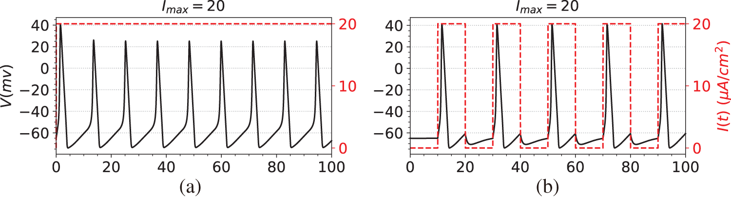
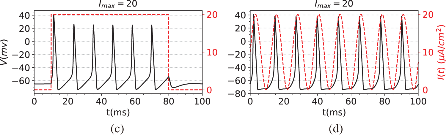
Figure 2: The dataset used in the simulation experiments. The black line is the membrane potential. The red line is the stimulating current. (a) Membrane potential induced by constant current stimulation. (b) Membrane potential induced by short pulse current stimulation. (c) Membrane potential induced by long-pulse current stimulation. (d) Membrane potential induced by sine function current stimulation

(a) A constant current, where

I(t)=20 μA/cm2.(25)

(b) A step function with a long pulse, such as

I(t)={0 μA/cm2,t∈[0,10),20 μA/cm2,t∈[10,80),0 μA/cm2,t∈[80,100).(26)

(c) A multi-pulse pulsing step function, such as

I(t)={0 μA/cm2,t∈[10q,10+10q),q=0,2,4,6,8,20 μA/cm2,t∈[10q,10+10q),q=1,3,5,7,9.(27)

(d) A sine function, such as

I(t)=10sin⁡(t2)+10 μA/cm2.(28)

CdVdt=I(t)−g¯Nam3h(V−ENa)−g¯Kn4(V−EK)−g¯L(V−EL),t0≤t≤tfinal ,(29)

dndt=αn(1−n)−βnn,(30)

dmdt=αm(1−m)−βmm,(31)

dhdt=αh(1−h)−βhh.(32)

αn=0.007 V+0.57,βn=−0.001 V+0.06,αm=0.636 V+4.431,βm=−0.061 V+0.468,αh=−0.01 V+0.009,βh=0.01 V+0.786.(33)

where C=1 μF/cm2, g¯Na=120 ms/cm2, g¯K=36 ms/cm2, g¯L=0.3 ms/cm2, ENa= 50 mV, EK=−77 mV, and EL=−54.387 mV. The initial values are V0=−65,n0=0.32,m0= 0.05, and h0=0.6.

Fig. 3 illustrates the prediction results of the parameters of the HH equation under constant current stimulation given by the conventional PINN (top row) and BioE-PINN (middle row) models. The first column presents the predicted results of Bβm and Aβm parameters. The second column presents the results of solving the HH equation according to the predicted parameters. In contrast to the fixed activation function, the parameters predicted by the adaptive activation function after 60,000 iterations are closest to the real values. The lower left graph shows a comparison of the loss functions of BioE-PINN and conventional PINN with a scale factor of 10. By introducing a scaling factor n and a learnable parameter a, the loss decreases faster. The optimal value of a is about 5.2, as shown in the lower right figure.

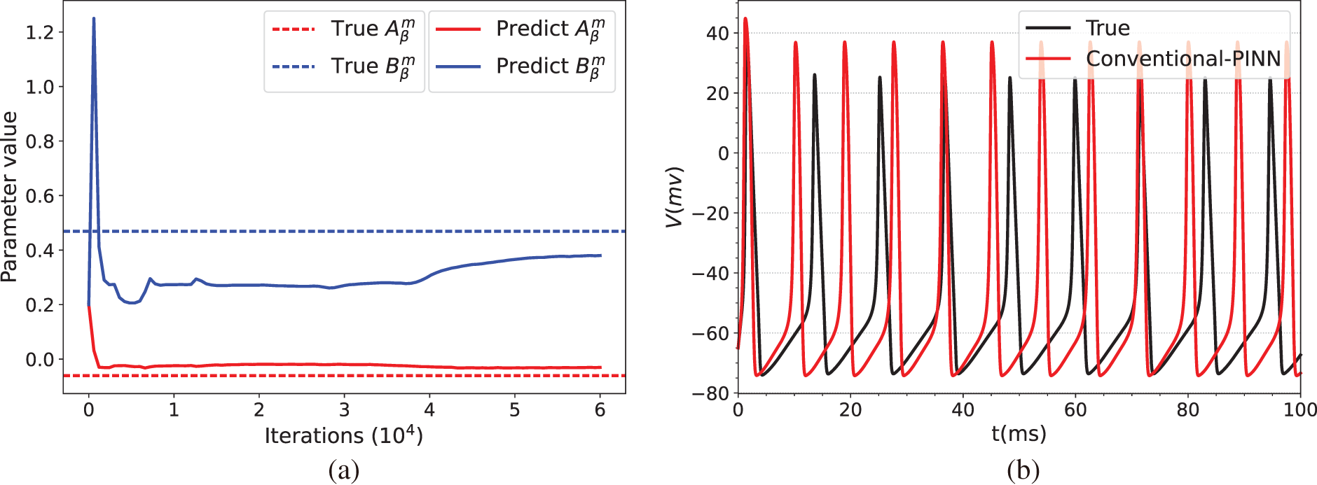
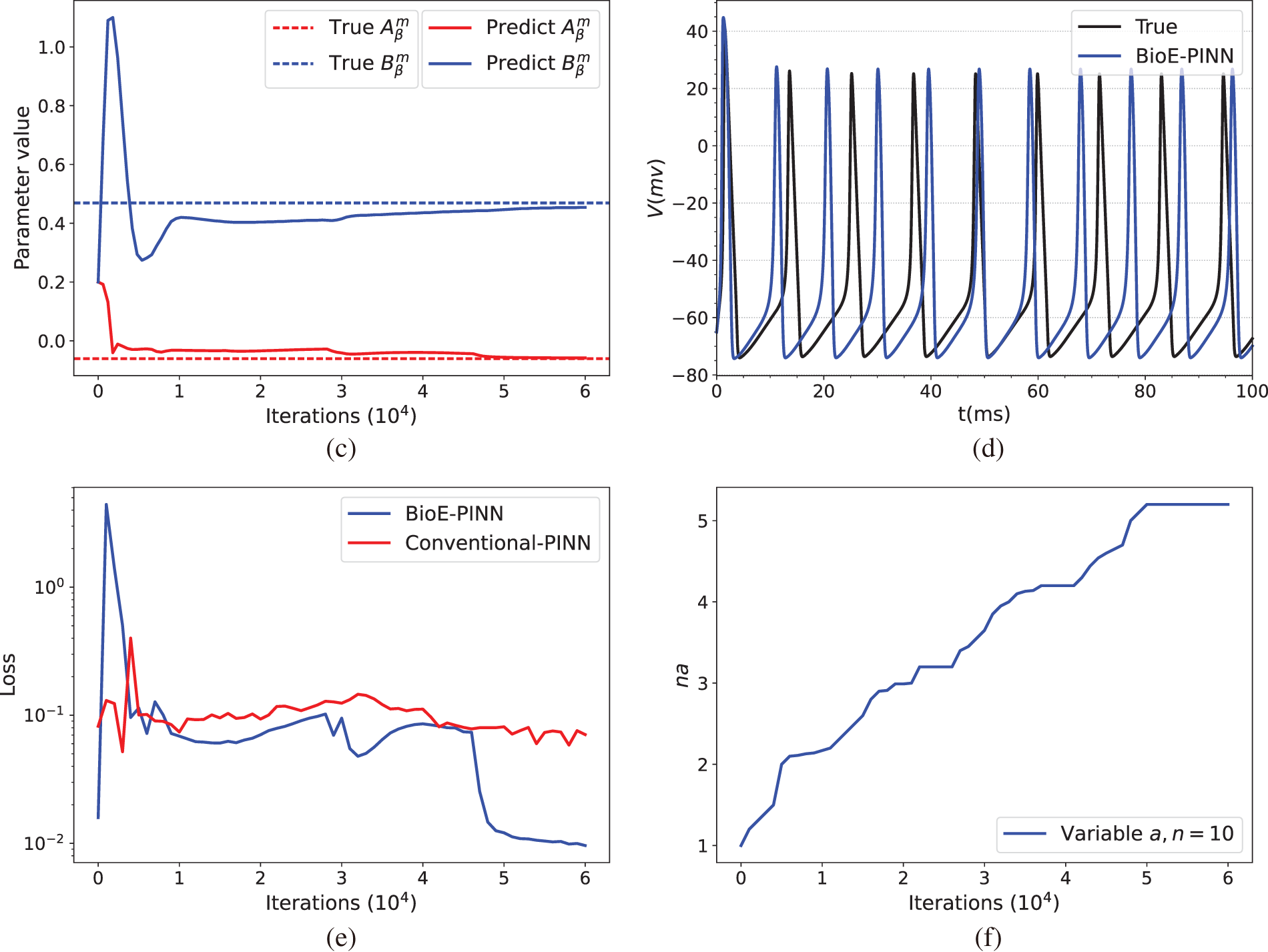
Figure 3: Prediction results under constant current stimulation. (a) and (c) show the parameter prediction results of Conventional-PINN and BioE-PINN, respectively. (b) and (d) present the results of solving the HH equation according to the predicted parameters. (e) shows the loss function change curve. (f) presents the change curve of the learnable parameter a

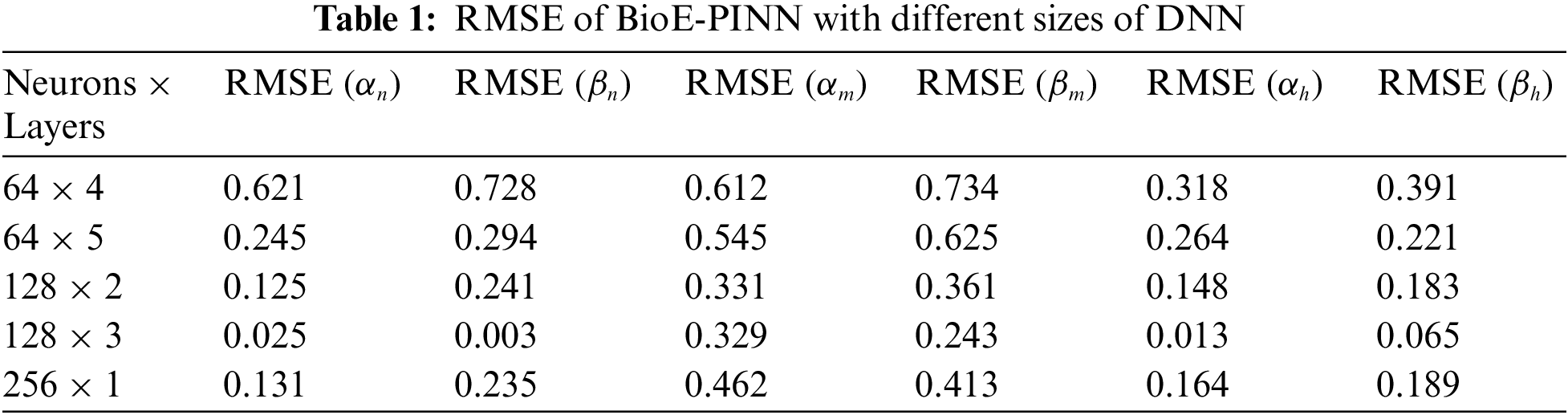
We briefly discuss the sensitivity of BioE-PINN to the number of neurons and layers of DNN models. The performance is found to be sensitive to the size of the DNN (neurons × number of layers), as shown in Table 1. The general trend is that deeper neural networks perform better by comparing the 64 × 4, 64 × 5, 128 × 2, and 128 × 3 cases, respectively. In this experiment, the architecture with 3 layers and 128 neurons per layer performs best.

The optimal structure of BioE-PINN is selected to predict the switch rate under different stimulation currents, and the results are shown in Table 2. It can be found that the predictive results of sinusoidal stimulation and short pulse stimulation are better than constant current stimulation and long pulse stimulation. Fig. 4 shows the relative error of the parameter prediction experiments. The black line in the figure reflects the fluctuation range of the error, and the red point is the average value. We can see that the average relative error of the 12 parameters is below 6%, reflecting the high stability of the model.

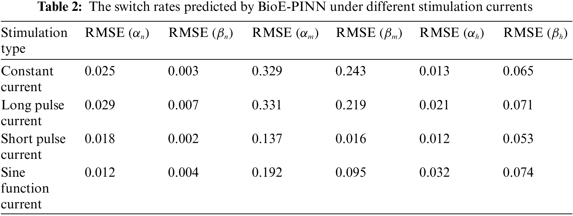
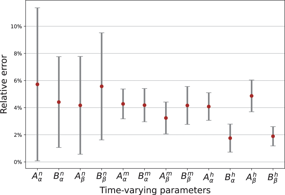
Figure 4: Relative error of parameters predicted by BioE-PINN. 10 experiments are performed, and the red dots are the average error values of the 10 experiments

Tables 3 and 4 show the predicted results of membrane potential and channel conductance. In detail, we solve the HH equation according to the parameters determined by BioE-PINN, and we can obtain the change curve of the membrane potential and the conductance of the ion channel, and calculate the respective RMSE and SPCC. Compared with RMSE, SPCC can reflect the changing trend of the curve. The larger the value of SPCC, the more similar the predicted value is to the real value, which can better reflect the physiological change process.

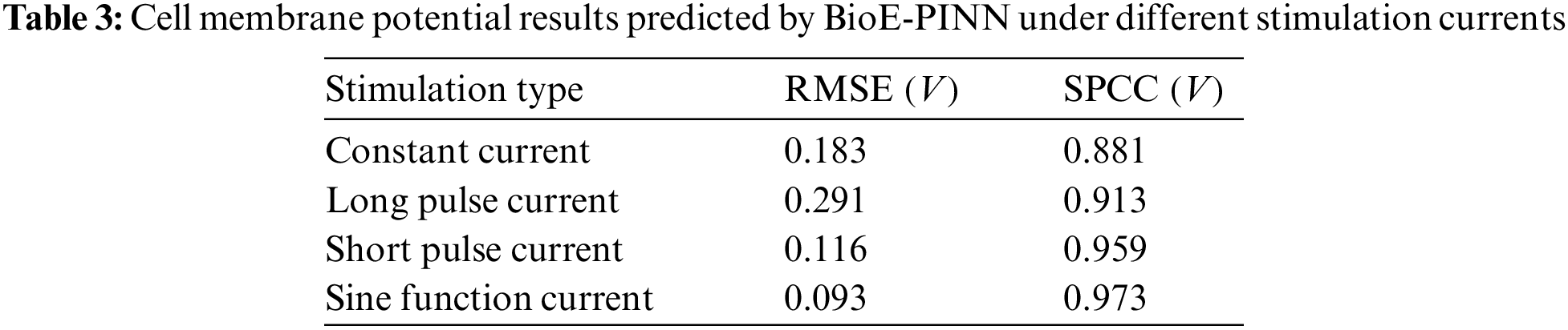
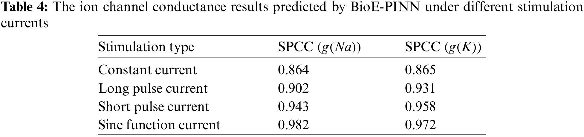
Table 5 shows the predicted results of the stimulation current. In this study, the prediction of the stimulation current is achieved through the fully connected layer. Fig. 5 shows the conductance and stimulation current predicted by BioE-PINN. It can be seen from the figure that the predicted change curve is basically consistent with the real value.

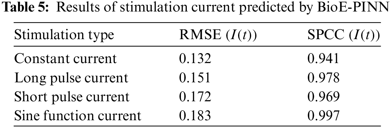
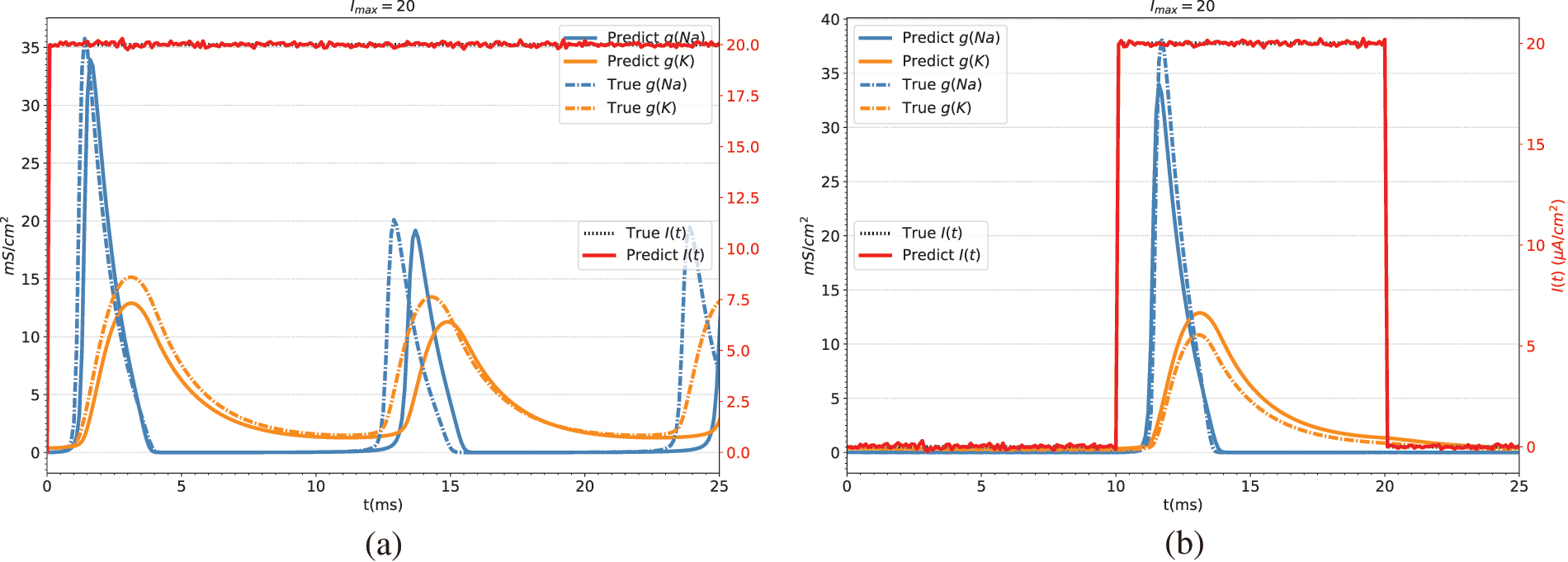
Figure 5: Conductance and stimulation current predicted by BioE-PINN. The red lines are the predicted stimulation currents. The blue and orange lines are the predicted sodium ion conductance and potassium ion conductance. The dotted line is the real value. (a) Predicted results of constant current stimulation. (b) Prediction results of short pulse current stimulation

4.2 Squid Giant Axon Membrane Potential Experiment

The squid giant axon is part of the squid’s jet propulsion control system. In 1952, after experiments on giant axons, Hodgkin and Huxley made assumptions about the dynamic characteristics of ion channels and uncovered the ion current mechanism of action potentials for the first time. Therefore, the BioE-PINN is also validated with the membrane potential data of the Squid giant axon and applied to predict the time-varying parameters and stimulation currents of the HH equation.

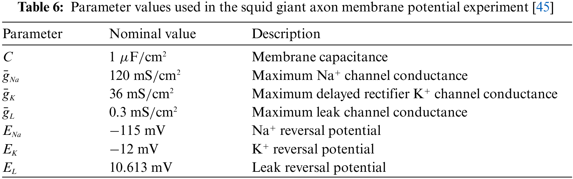
Specifically, we first use the Eqs. (29)–(32) to construct the loss function (Eq. (10)). Then generate a time series t as the input of BioE-PINN, the length of t is 200, and the range is [0, 2]. In addition, the membrane potential recorded in the experiment is used to calculate data-driven loss (Eq. (11)), and the parameter settings in the equation are shown in Table 6.

Eq. (34) are the ion channel dynamics characteristics predicted by BioE-PINN. The predicted parameters are used to compute the numerical solution of Eq. (29), and the results are shown in Fig. 6. Fig. 6 presents the measured membrane potential (black line), predicted membrane potential (blue line), and predicted stimulation current (red line). It can be seen from the figure that our method can predict action potentials efficiently, and the Pearson coefficient and RMSE of the predicted value and the real value are 0.89 and 0.18, respectively. Based on the experimental results, we found that there is a change in the stimulation current, which decreases rapidly during the depolarization phase of the electrical signal.

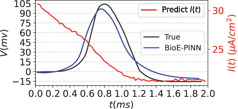
Figure 6: Prediction results of squid giant axon membrane potential. The real data is from Fig. 15C in the literature [45]. The blue line is the predicted electrical signal. The red line is the predicted stimulation current

αn(V)=0.012 V+0.286,βn(V)=−0.05 V+0.16,αm(V)=0.263 V+15.23,βm(V)=0.168 V+1.367,αh(V)=0.01 V+12.91,βh(V)=0.1 V+87.86.(34)

Fig. 7 illustrates the predicted results of the ion channel conductance. The left Fig. 7a is the conductance change curve predicted by BioE-PINN. The Fig. 7b is the experimentally recorded change curve of the conductance of the sodium ion channel from the literature [45]. By comparing the two, it can be found that the change trend of sodium conductance we predicted is close to that of the experiment, and it rises rapidly in the depolarization stage.

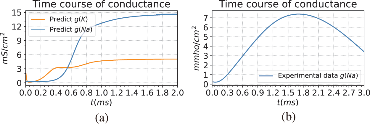
Figure 7: Giant squid axon conductance predicted by BioE-PINN. (a) Result of model prediction. The blue and orange lines in the figure are the predicted potassium ion conductance and sodium ion conductance, namely g(K)=n4, g(Na)=g¯Nam3h. (b) The change curve of sodium conductance calculated from the voltage-clamp experiment

4.3 Plant Cell Membrane Potential Experiment

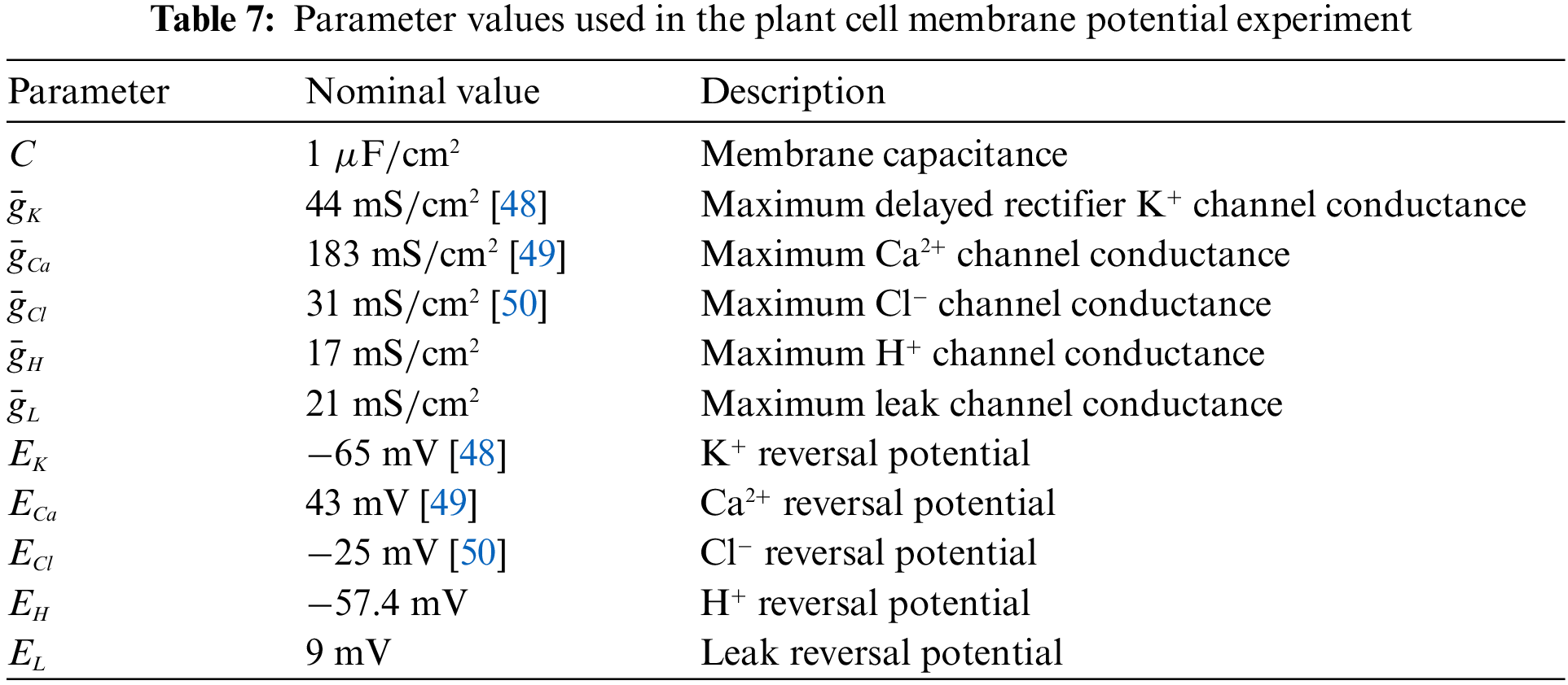
The PINN-based framework can be used to solve the HH equation and determine the parameters in the equation. This allows us to try this method for model solving of plant electrical signals. Plant electrical signaling is a rather complex process, and the ion channels involved in its formation have not been fully discovered. Therefore, it is of great significance to help biologists to discover the dynamic characteristics of plant ion channels using computational methods. At present, scientists have found potassium, calcium, chloride, and hydrogen ions in the cell membranes of higher plants. Based on previous studies [46], this paper advances the HH equation to describe the membrane potential of Arabidopsis mesophyll cells, as Eq. (35), and the parameters of the equation are set in Table 7. To be more specific, we empirically determined the membrane potential model of Arabidopsis mesophyll cells through trial and error.

The Arabidopsis mesophyll cell membrane potential data in Fig. 3b in the literature [47] are exploited to conduct experiments, shown in the first column of Fig. 8, which record the cellular electrical activity of mesophyll cells stimulated by blue light. In detail, we first determine the stimulation current I(t) and time-varying parameters in the mesophyll cell membrane potential model using BioE-PINN, and then solve Eq. (35) using the predicted parameters.

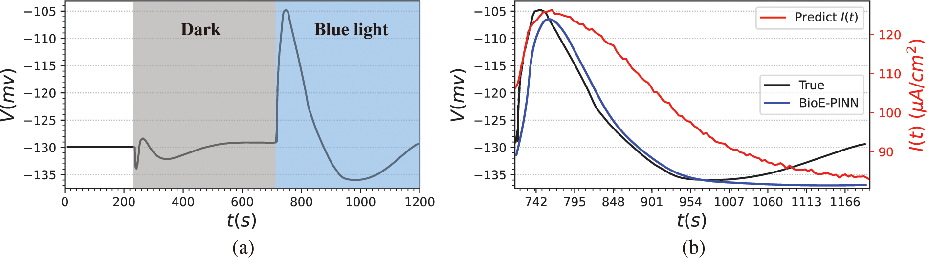
Figure 8: The mesophyll cell membrane potential of Arabidopsis induced by blue light. (a) Raw data from the literature. 713–1200 s stimulated by blue light. (b) Prediction results of BioE-PINN. The black lines are the real electrical signal values, the blue lines are the predicted electrical signals, and the red lines are the predicted stimulus currents

The second column of Fig. 8 shows the measured membrane potential (black line), predicted membrane potential (blue line), and predicted stimulation current (red line). It can be found from the figure that in the depolarization stage, the predicted electrical signal changes slowly and fails to reach the same extreme value as the measured data quickly. From the evaluation indicators, the Pearson coefficient and RMSE of the predicted value and the real value are 0.86 and 0.2, respectively. We believe that the predicted parameters can better reflect the changes of plant membrane potential. The stimulating current reflects the change process of all charged substances in the cells after the plant is stimulated, and the current generated by these substances further induces changes in the membrane potential of the mesophyll cell. According to the experimental phenomenon, it is speculated that the light intensity of this biological experiment does not reach the threshold for generating action potentials, or it is a subthreshold local potential, since we do not predict the continuous AP signal based on the experimental results.

The current mechanism of ions involved in the formation of electrical signals in plants needs to be further studied. There are many mechanistic models that cause plant electrical activity, but each parameter of a model often comes from different plants [51,52]. For the description of plant electrical phenomena, its generalization needs to be improved. Our method models plant electrical signals based on reasonable assumptions, and the prediction results show that the model can well predict the light-induced membrane potential. To further demonstrate the interpretability and reliability of the model, the predicted conductivities of ion channels are analyzed, namely g(K)=g¯Kn4, g(Ca)=g¯Cam3, g(Cl)=g¯Clm2h and g(H)=g¯Hh.

To further verify the reliability of the model, we derived the conductance change curves of potassium and chloride channels from patch-clamp data extracted from the literature. Specifically, the whole-cell voltage clamp data in [53] and [54] are employed to obtain the current values under different clamping voltages. g(t) can be calculated according to g=I/(V−E). Next, we describe the conductance of the potassium channel as:

g(K)=g¯Kn4,(36)

dndt=αn(1−n)−βnn.(37)

where g(K) is the potassium channel conductance, which is related to time and membrane potential. g¯K is the maximum conductance of the channel. The value of n when the cell is in a resting state can be expressed as:

n0=αn0αn0+βn0.(38)

When the membrane potential changes, it can be obtained from Eq. (37):

n=n∞−(n∞−n0)e−tτn.(39)

We bring Eqs. (39) into (36) to obtain Eq. (40), and then use the conductance data at each clamp potential to calculate their respective τn. Next, we calculate n∞, where the maximum conductance of the potassium channel is 44 mS/cm2. Finally, the switch rates αn and βn of n are calculated from these parameters:

g(K)=[g∞−(g∞−g0)e−tτn]4.(40)

where g∞ and g0 can be obtained from experimental data. In this paper, it is assumed that n∞=αn/(αn+βn), τn=1/(αn+βn).

The above equation is applied to find the switch rate of the activation factor n at each clamp potential, and then Eqs. (41) and (42) are utilized to fit it. Similarly, the switch rate of the chlorine channel according to the above method is calculated. For the detailed calculation process and results, please refer to the appendix. The final calculated conductivity is shown in Fig. 9b. The conductivities derived manually and predicted by BioE-PINN are compared, and it is found that the numerical ranges of the two are not consistent. The overall value of the conductivity predicted by BioE-PINN is relatively small. The reason for this phenomenon may be that the switch rate equations predicted and deduced from real data are different. To be more specific, the switch rate equations set in BioE-PINN are shown in Eqs. (6) and (7), which differ from Eqs. (41) and (42). Accordingly, the initial value of conductivity will be different. However, the results of prediction and artificial derivation show that the conductivity of the potassium channel increases rapidly within the time period of 50–200 s, indicating that there are a large number of potassium ions in and out of the channel. Therefore, our predicted potassium channel conductivity is basically consistent with the results deduced from experimental data.

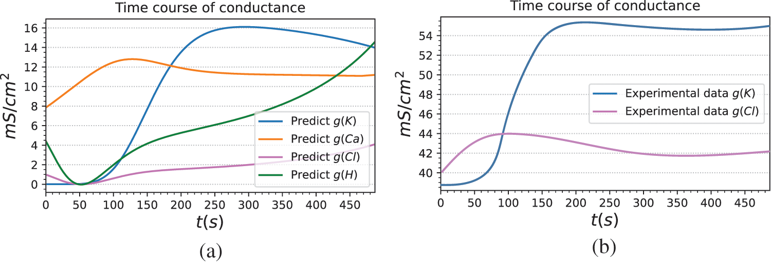
Figure 9: Ion channel and proton pump conductance predicted by BioE-PINN. (a) The ion channel and proton pump conductance curves of Arabidopsis mesophyll cells predicted by BioE-PINN. (b) Whole-cell voltage-clamp data from literature [53] and literature [54] are used, and the conductance curves of potassium and chloride channels are manually derived according to Eq. (35)

αn=(cV+d)aeVb.(41)

βn=(cV+d)aeVb.(42)

where a, b, c and d are all free parameters, which can be calculated by the least square method.

5  Conclusion

In this paper, we developed a framework for identifying the time-varying parameters of physiological equations based on improved PINN, which integrates the electrophysiological equations into the loss function of the neural network and adds hard constraints to make the predicted output of the neural network conform to physical laws. The difference between our framework and traditional PINN is that we add an adaptive activation function to improve the accuracy of the model and slow down the convergence. Finally, simulation experiments prove that BioE-PINN can predict the dynamic characteristics of ion channels and pumps by using membrane potential, such as gating variables, conductivity and other parameters. At the same time, we verified the effectiveness and accuracy of the model with real electrical signal data of animals and plants. In future work, it is possible to consider more complex physiological equation modeling. In addition, how to promote BioE-PINN to different fields to obtain application value is also worth studying.

Funding Statement: This work was supported by the National Natural Science Foundation of China under 62271488 and 61571443.

Conflicts of Interest: The authors declare that they have no known competing financial interests or personal relationships that could have appeared to influence the work reported in this paper.

References

1. Akinfe, K. T., Loyinmi, A. C. (2022). The implementation of an improved differential transform scheme on the schrodinger equation governing wave-particle duality in quantum physics and optics. Results in Physics, 40(1), 105806. https://doi.org/10.1016/j.rinp.2022.105806 [Google Scholar] [CrossRef]

2. Fareed, A. F., Semary, M. S., Hassan, H. N. (2022). Two semi-analytical approaches to approximate the solution of stochastic ordinary differential equations with two enormous engineering applications. Alexandria Engineering Journal, 61(12), 11935–11945. https://doi.org/10.1016/j.aej.2022.05.054 [Google Scholar] [CrossRef]

3. Amigo, J. M., Small, M. (2017). Mathematical methods in medicine: Neuroscience, cardiology and pathology. Philosophical Transactions of the Royal Society A: Mathematical, Physical and Engineering Sciences, 375(2096), 20170016. https://doi.org/10.1098/rsta.2017.0016 [Google Scholar] [PubMed] [CrossRef]

4. Lagergren, J. H., Nardini, J. T., Michael Lavigne, G., Rutter, E. M., Flores, K. B. (2020). Learning partial differential equations for biological transport models from noisy spatio-temporal data. Proceedings of the Royal Society A: Mathematical, Physical and Engineering Sciences, 476(2234), 20190800. https://doi.org/10.1098/rspa.2019.0800 [Google Scholar] [PubMed] [CrossRef]

5. Higgins, J. P. (2002). Nonlinear systems in medicine. The Yale Journal of Biology and Medicine, 75(5–6), 247–260. [Google Scholar] [PubMed]

6. Metwally, A. S., El-Sheikh, S. M. A., Galal, A. A. A. (2022). The impact of diabetes mellitus on the pharmacokinetics of rifampicin among tuberculosis patients: A systematic review and meta-analysis study. Diabetes & Metabolic Syndrome: Clinical Research & Reviews, 16(2), 102410. https://doi.org/10.1016/j.dsx.2022.102410 [Google Scholar] [PubMed] [CrossRef]

7. Cheng, V., Abdul-Aziz, M. H., Burrows, F., Buscher, H., Cho, Y. J. et al. (2022). Population pharmacokinetics and dosing simulations of ceftriaxone in critically ill patients receiving extracorporeal membrane oxygenation (an ASAP ECMO study). Clinical Pharmacokinetics, 61(6), 847–856. https://doi.org/10.1007/s40262-021-01106-x [Google Scholar] [PubMed] [CrossRef]

8. Hodgkin, A. L., Huxley, A. F. (1952). The dual effect of membrane potential on sodium conductance in the giant axon of Loligo. The Journal of Physiology, 116(4), 497–506. https://doi.org/10.1113/jphysiol.1952.sp004719 [Google Scholar] [PubMed] [CrossRef]

9. Wang, J., Li, T. F., Sun, C., Yan, R. Q., Chen, X. F. (2022). Improved spiking neural network for intershaft bearing fault diagnosis. Journal of Manufacturing Systems, 65(1), 208–219. https://doi.org/10.1016/j.jmsy.2022.09.003 [Google Scholar] [CrossRef]

10. Lok, L. C., Mirams, G. R. (2021). Neural network differential equations for ion channel modelling. Frontiers in Physiology, 12(1), 708944. https://doi.org/10.3389/fphys.2021.708944 [Google Scholar] [PubMed] [CrossRef]

11. Türkyilmazoğlu, M. (2022). An efficient computational method for differential equations of fractional type. Computer Modeling in Engineering & Sciences, 133(1), 47–65. https://doi.org/10.32604/cmes.2022.020781 [Google Scholar] [CrossRef]

12. Blechschmidt, J., Ernst, O. G. (2021). Three ways to solve partial differential equations with neural networks-a review. GAMM-Mitteilungen, 44(2), e202100006. https://doi.org/10.1002/gamm.202100006 [Google Scholar] [CrossRef]

13. Karniadakis, G. E., Kevrekidis, I. G., Lu, L., Paris, P., Sifan, W. et al. (2021). Physics-informed machine learning. Nature Reviews Physics, 3(6), 422–440. https://doi.org/10.1038/s42254-021-00314-5 [Google Scholar] [CrossRef]

14. Roy, A. M., Bose, R., Sundararaghavan, V., Arróyave, R. (2023). Deep learning-accelerated computational framework based on physics informed neural network for the solution of linear elasticity. Neural Networks, 162(1), 472–489. https://doi.org/10.1016/j.neunet.2023.03.014 [Google Scholar] [PubMed] [CrossRef]

15. Pang, H., Wu, L., Liu, J., Liu, X., Liu, K. (2023). Physics-informed neural network approach for heat generation rate estimation of lithium-ion battery under various driving conditions. Journal of Energy Chemistry, 78(1), 1–12. https://doi.org/10.1016/j.jechem.2022.11.036 [Google Scholar] [CrossRef]

16. Herrero, M. C., Oved, A., Bharath, A. A., Varela, M. (2022). EP-PINNs: Cardiac electrophysiology characterisation using physics-informed neural networks. Frontiers in Cardiovascular Medicine, 8(1), 768419. https://doi.org/10.3389/fcvm.2021.768419 [Google Scholar] [PubMed] [CrossRef]

17. Psaros, A. F., Kawaguchi, K., Karniadakis, G. E. (2022). Meta-learning PINN loss functions. Journal of Computational Physics, 458(1), 111121. https://doi.org/10.1016/j.jcp.2022.111121 [Google Scholar] [CrossRef]

18. Qin, X., Liu, Z., Liu, Y., Liu, S., Yang, B. et al. (2022). User ocean personality model construction method using a BP neural network. Electronics, 11(19), 3022. https://doi.org/10.3390/electronics11193022 [Google Scholar] [CrossRef]

19. Lu, S., Guo, J., Liu, S., Yang, B., Liu, M. et al. (2022). An improved algorithm of drift compensation for olfactory sensors. Applied Sciences, 12(19), 9529. https://doi.org/10.3390/app12199529 [Google Scholar] [CrossRef]

20. Dang, W., Guo, J., Liu, M., Liu, S., Yang, B. et al. (2022). A semi-supervised extreme learning machine algorithm based on the new weighted kernel for machine smell. Applied Sciences, 12(18), 9213. https://doi.org/10.3390/app12189213 [Google Scholar] [CrossRef]

21. Raissi, M., Perdikaris, P., Karniadakis, G. E. (2019). Physics-informed neural networks: A deep learning framework for solving forward and inverse problems involving nonlinear partial differential equations. Journal of Computational Physics, 378, 686–707. https://doi.org/10.1016/j.jcp.2018.10.045 [Google Scholar] [CrossRef]

22. Jagtap, A. D., Kawaguchi, K., Karniadakis, G. E. (2020). Adaptive activation functions accelerate convergence in deep and physics-informed neural networks. Journal of Computational Physics, 404(4), 109136. https://doi.org/10.1016/j.jcp.2019.109136 [Google Scholar] [CrossRef]

23. Yu, J., Lu, L., Meng, X., Karniadakis, G. E. (2022). Gradient-enhanced physics-informed neural networks for forward and inverse PDE problems. Computer Methods in Applied Mechanics and Engineering, 393(6), 114823. https://doi.org/10.1016/j.cma.2022.114823 [Google Scholar] [CrossRef]

24. Wu, C., Zhu, M., Tan, Q., Kartha, Y., Lu, L. (2023). A comprehensive study of non-adaptive and residual-based adaptive sampling for physics-informed neural networks. Computer Methods in Applied Mechanics and Engineering, 403(1), 115671. https://doi.org/10.1016/j.cma.2022.115671 [Google Scholar] [CrossRef]

25. Lu, L., Meng, X., Mao, Z., Karniadakis, G. E. (2021). DeepXDE: A deep learning library for solving differential equations. SIAM Review, 63(1), 208–228. https://doi.org/10.1137/19M1274067 [Google Scholar] [CrossRef]

26. Hennigh, O., Narasimhan, S., Nabian, M. A., Subramaniam, A., Tangsali, K. et al. (2021). NVIDIA SIMNET: An AI-accelerated multi-physics simulation framework. International Conference on Computational Science, Poland, Springer. [Google Scholar]

27. Chen, F., Sondak, D., Protopapas, P., Mattheakis, M., Liu, S. et al. (2020). NeuroDiffEq: A python package for solving differential equations with neural networks. Journal of Open Source Software, 5(46), 1931. https://doi.org/10.21105/joss.01931 [Google Scholar] [CrossRef]

28. Haghighat, E., Juanes, R. (2021). SciANN: A Keras/Tensorflow wrapper for scientific computations and physics-informed deep learning using artificial neural networks. Computer Methods in Applied Mechanics and Engineering, 373(7553), 113552. https://doi.org/10.1016/j.cma.2020.113552 [Google Scholar] [CrossRef]

29. Yuan, L., Ni, Y. Q., Deng, X. Y., Hao, S. (2022). A-PINN: Auxiliary physics informed neural networks for forward and inverse problems of nonlinear integro-differential equations. Journal of Computational Physics, 462, 111260. https://doi.org/10.1016/j.jcp.2022.111260 [Google Scholar] [CrossRef]

30. Shukla, K., Jagtap, A. D., Blackshire, J. L., Sparkman, D., Karniadakis, G. E. (2021). A physics-informed neural network for quantifying the microstructural properties of polycrystalline nickel using ultrasound data: A promising approach for solving inverse problems. IEEE Signal Processing Magazine, 39(1), 68–77. https://doi.org/10.1109/MSP.2021.3118904 [Google Scholar] [CrossRef]

31. Chen, D., Gao, X., Xu, C., Wang, S., Chen, S. et al. (2022). FlowDNN: A physics-informed deep neural network for fast and accurate flow prediction. Frontiers of Information Technology & Electronic Engineering, 23(2), 207–219. https://doi.org/10.1631/FITEE.2000435 [Google Scholar] [CrossRef]

32. Jagtap, A. D., Mao, Z., Adams, N., Karniadakis, G. E. (2022). Physics-informed neural networks for inverse problems in supersonic flows. Journal of Computational Physics, 466(1), 111402. https://doi.org/10.1016/j.jcp.2022.111402 [Google Scholar] [CrossRef]

33. Xie, J., Yao, B. (2022). Physics-constrained deep learning for robust inverse ECG modeling. IEEE Transactions on Automation Science and Engineering, 20(1), 151–166. https://doi.org/10.1109/TASE.2022.3144347 [Google Scholar] [CrossRef]

34. Herrero Martin, C., Oved, A., Chowdhury, R. A., Ullmann, E., Peters, N. S. et al. (2022). EP-PINNs: Cardiac electrophysiology characterisation using physics-informed neural networks. Frontiers in Cardiovascular Medicine, 2179, 768419. https://doi.org/10.3389/fcvm.2021.768419 [Google Scholar] [PubMed] [CrossRef]

35. Jariwala, P., Jadhav, K. (2022). The safety and efficacy of efonidipine, an L- and T-type dual calcium channel blocker, on heart rate and blood pressure in indian patients with mild-to-moderate essential hypertension. European Heart Journal, 43(1), 143–849. https://doi.org/10.1093/eurheartj/ehab849.143 [Google Scholar] [CrossRef]

36. Liu, C., Liu, X., Liu, S. (2014). Bifurcation analysis of a morris–lecar neuron model. Biological Cybernetics, 108(1), 75–84. https://doi.org/10.1007/s00422-013-0580-4 [Google Scholar] [PubMed] [CrossRef]

37. Lei, C. L., Mirams, G. R. (2021). Neural network differential equations for ion channel modelling. Frontiers in Physiology, 12, 708944. https://doi.org/10.3389/fphys.2021.708944 [Google Scholar] [PubMed] [CrossRef]

38. Ji, W., Qiu, W., Shi, Z., Pan, S., Deng, S. (2021). Stiff-PINN: Physics-informed neural network for stiff chemical kinetics. The Journal of Physical Chemistry A, 125(36), 8098–8106. https://doi.org/10.1021/acs.jpca.1c05102 [Google Scholar] [PubMed] [CrossRef]

39. Bienstock, D., Muñoz, G., Pokutta, S. (2018). Principled deep neural network training through linear programming. arXiv preprint arXiv: 1810.03218. [Google Scholar]

40. Zhang, M., Hibi, K., Inoue, J. (2023). GPU-accelerated artificial neural network potential for molecular dynamics simulation. Computer Physics Communications, 108655. https://doi.org/10.1016/j.cpc.2022.108655 [Google Scholar] [CrossRef]

41. Paszke, A., Gross, S., Chintala, S., Chanan, G., Yang, E. et al. (2017). Automatic differentiation in pytorch. NIPS 2017 Autodiff Workshop: The Future of Gradient-Based Machine Learning Software and Techniques, Long Beach, CA, USA. [Google Scholar]

42. Glorot, X., Bengio, Y. (2010). Understanding the difficulty of training deep feedforward neural networks. Proceedings of the Thirteenth International Conference on Artificial Intelligence and Statistics. JMLR Workshop and Conference Proceedings, pp. 249–256. Chia Laguna Resort, Sardinia, Italy. [Google Scholar]

43. Kingma, D. P., Ba, J. (2014). ADAM: A method for stochastic optimization. arXiv preprint arXiv: 1412.6980. [Google Scholar]

44. Virtanen, P., Gommers, R., Oliphant, T. E., Haberland, M., Reddy, T. et al. (2020). SciPy 1.0: Fundamental algorithms for scientific computing in Python. Nature Methods, 17(3), 261–272. https://doi.org/10.1038/s41592-019-0686-2 [Google Scholar] [PubMed] [CrossRef]

45. Hodgkin, A. L., Huxley, A. F. (1952). A quantitative description of membrane current and its application to conduction and excitation in nerve. The Journal of Physiology, 117(4), 500–544. https://doi.org/10.1113/jphysiol.1952.sp004764 [Google Scholar] [PubMed] [CrossRef]

46. Wang, Z., Huang, L., Yan, X., Wang, C., Xu, Z. et al. (2007). A theory model for description of the electrical signals in plant part I. International Conference on Computer and Computing Technologies in Agriculture, Wuyishan, China, Springer. [Google Scholar]

47. Marten, I., Deeken, R., Hedrich, R., Roelfsema, M. (2010). Light-induced modification of plant plasma membrane ion transport. Plant Biology, 12, 64–79. https://doi.org/10.1111/j.1438-8677.2010.00384.x [Google Scholar] [PubMed] [CrossRef]

48. Spalding, E. P., Slayman, C. L., Goldsmith, M. H. M., Gradmann, D., Bertl, A. (1992). Ion channels in Arabidopsis plasma membrane: Transport characteristics and involvement in light-induced voltage changes. Plant Physiology, 99(1), 96–102. [Google Scholar] [PubMed]

49. de Angeli, A., Moran, O., Wege, S., Filleur, S., Ephritikhine, G. et al. (2009). ATP binding to the c terminus of the Arabidopsis thaliana nitrate/proton antiporter, atclca, regulates nitrate transport into plant vacuoles. Journal of Biological Chemistry, 284(39), 26526–26532. [Google Scholar] [PubMed]

50. Lew, R. R. (1991). Substrate regulation of single potassium and chloride ion channels in Arabidopsis plasma membrane. Plant Physiology, 95(2), 642–647. [Google Scholar] [PubMed]

51. Vodeneev, V., Orlova, A., Morozova, E., Orlova, L., Akinchits, E. et al. (2012). The mechanism of propagation of variation potentials in wheat leaves. Journal of Plant Physiology, 169(10), 949–954. [Google Scholar] [PubMed]

52. Sukhova, E., Akinchits, E., Sukhov, V. (2017). Mathematical models of electrical activity in plants. The Journal of Membrane Biology, 250(5), 407–423. [Google Scholar] [PubMed]

53. Reintanz, B., Szyroki, A., Ivashikina, N., Ache, P., Godde, M. et al. (2002). AtKC1, a silent Arabidopsis potassium channel α-subunit modulates root hair k+ influx. Proceedings of the National Academy of Sciences, 99(6), 4079–4084. [Google Scholar]

54. Qi, Z., Kishigami, A., Nakagawa, Y., Iida, H., Sokabe, M. (2004). A mechanosensitive anion channel in Arabidopsis thaliana mesophyll cells. Plant and Cell Physiology, 45(11), 1704–1708. [Google Scholar] [PubMed]