
 Submit a Paper
 Propose a Special lssue
 Open Access
ARTICLE
The Weighted Basis for PHT-Splines
1 School of Mathematical Sciences, Soochow University, Suzhou, 215006, China
2 School of Mathematical Sciences, University of Science and Technology of China, Hefei, 230026, China
* Corresponding Author: Falai Chen. Email:
(This article belongs to the Special Issue: Integration of Geometric Modeling and Numerical Simulation)
Computer Modeling in Engineering & Sciences 2024, 138(1), 739-760. https://doi.org/10.32604/cmes.2023.027171
Received 17 October 2022; Accepted 03 January 2023; Issue published 22 September 2023
 View Full Text
 Download PDF
Abstract
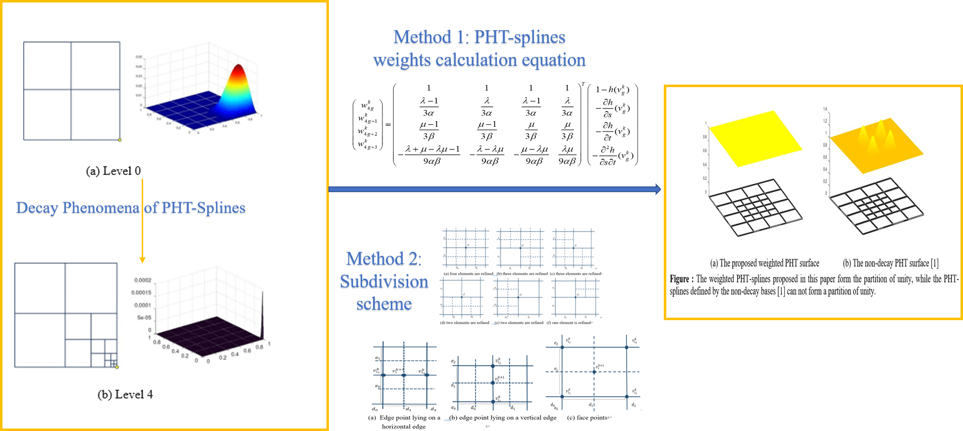
PHT-splines are defined as polynomial splines over hierarchical T-meshes with very efficient local refinement properties. The original PHT-spline basis functions constructed by the truncation mechanism have a decay phenomenon, resulting in numerical instability. The non-decay basis functions are constructed as the B-splines that are defined on the 2 × 2 tensor product meshes associated with basis vertices in Kang et al., but at the cost of losing the partition of unity. In the field of finite element analysis and topology optimization, forming the partition of unity is the default ingredient for constructing basis functions of approximate spaces. In this paper, we will show that the non-decay PHT-spline basis functions proposed by Kang et al. can be appropriately modified to form a partition of unity. Each non-decay basis function is multiplied by a positive weight to form the weighted basis. The weights are solved such that the sum of weighted bases is equal to 1 on the domain. We provide two methods for calculating weights, based on geometric information of basis functions and the subdivision of PHT-splines. Weights are given in the form of explicit formulas and can be efficiently calculated. We also prove that the weights on the admissible hierarchical T-meshes are positive.Graphic Abstract
Keywords
Polynomial splines over hierarchical T-meshes (PHT-splines for short) [1] are a kind of global
With further in-depth application, the improvement of PHT-splines has also been underway. One of the limitations of PHT-splines is the restrictions from hierarchical T-meshes, which require the underlying meshes to start with tensor product meshes and be refined by inserting crosses. The generalization of PHT-splines on general T-meshes [15] and modified hierarchical T-meshes (allowing split-in-half in mesh refinement) [16] is precisely aimed at overcoming the restrictions from meshes. Another improvement regard to PHT-splines is the construction of basis functions. The original basis functions [1] have a decay phenomenon (the function values decay as the level increases) when the level difference is big in the underlying support. The decay of basis functions when applied in iso-geometric analysis leads to ill-conditioned stiffness matrices, and thus unstable numerical solutions. A new set of basis functions is defined by the B-splines that defined on the 2 × 2 tensor product meshes associated with basis vertices [2] to overcome the decay phenomenon that occurs in basis functions, but at the cost of losing the partition of unity.
The partition of unity is a default ingredient in the construction of approximating functions in finite element methods [17–19]. Moreover, in the field of topology optimization [14], the density variable takes value in the range of
The truncation mechanism is a common way of constructing basis functions for hierarchical spline spaces that form a partition of unity, such as the original PHT-splines [1], THB-splines (the truncated hierarchical B-splines) [20] and truncated T-splines [21]. But as mentioned above, the truncation mechanism causes the decay in basis functions. In this paper, we will show that the basis functions that form the partition of unity and have no decay can be constructed without the truncation mechanism. The weighted bases that satisfy the required properties are defined by the bases constructed in [2] multiplied by positive weights. The weight for each basis function can be computed explicitly and efficiently based on the geometric information of the basis function. Moreover, when the level difference is not greater than 2, the weights can also be computed by the PHT subdivision scheme.
In [22], the authors also proposed a method to define new basis functions to overcome the decay problem and guarantee the partition of unity. However, their method only considers specific cases that the original truncated basis functions have rectangular supports, in which case they are replaced by the associated tensor product B-splines. Instead, our method is more versatile and can be applied to arbitrary T-meshes easily.
The rest of this paper is organized as follows. In Section 2, some basics of PHT-splines are reviewed. In Section 3, we introduce the weighted bases in detail. In Section 4, the subdivision scheme of PHT-splines is introduced as an alternative algorithm for calculating weights. In Section 5, some hierarchical T-meshes are demonstrated to verify the effectiveness of the proposed method. Finally, we conclude the paper with a summary in Section 6.
In this section, we give a brief review of the definition of PHT-splines. The readers are recommended to refer to [1] for more details.
Given a T-mesh
where
PHT is defined by
The dimension formula of PHT has a concise expression with
where
The original PHT basis functions are constructed by truncation mechanism in [1] level by level in order to make basis functions vanish at other basis vertices. Fig. 1 shows two typical hierarchical meshes, where the basis functions associated the marked vertices have undesired decay as level increases. In Fig. 1a, the maximum values decay rapidly as the level increases. In Fig. 1b, the maximum value does not decrease, but the basis function decays sharply along the refinement direction as level increases. This decay phenomenon of basis functions is first noted in [2]. The decay phenomenon makes the stiffness matrix have large condition number and thus produces unstable solutions.

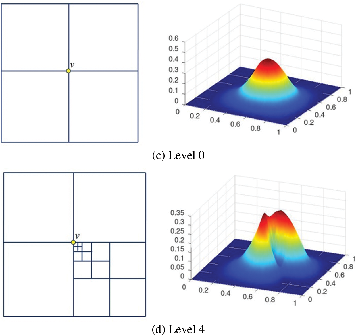
Figure 1: The decay phenomenon of PHT-spline basis functions associated with the vertex marked by a yellow circle
A new basis functions are proposed in [2] to amend the decay phenomenon. In the following, we give a brief review of the construction.
Definition 1 Suppose
Note that if
Fig. 2 illustrates the support meshes of six basis vertices including three boundary vertices and three interior crossing vertices, where the six basis vertices are marked by solid circles and the corresponding support meshes are marked by bold lines.
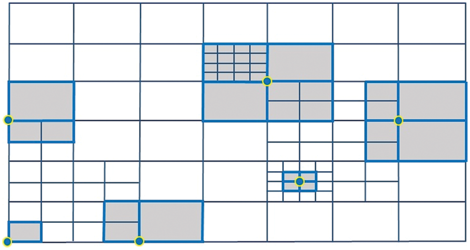
Figure 2: Support meshes of six basis vertices
The basis functions associated with a basis vertex are then defined by the four B-spline functions that defined on the support mesh. Specifically, for a basis vertex
These four basis functions are linearly independent and have the same support
3 Weighted Bases for PHT-Splines
For any basis function
For a basis vertex
where
The sum of the geometric information of the four basis functions
Suppose that the maximal subdivision level of
According to the definitions of support meshes and hierarchical T-meshes, the basis function proposed in [2] has the following property:
• A basis vertex at level
where
• The basis functions
The proposed weighted bases are defined by multiplying the basis functions constructed in [2] by positive weights. This ensures that the weighted bases not only have no decay, but also form the positive partition of unity. In the following, we are going to compute weights
This problem can be understood as the PHT fitting problem of a constant function. Since a PHT-spline space spans the bicubic polynomial space
The weights are computed level by level. First, we evaluate the PHT-spline surface at the basis vertices on level 0, that is
since the basis functions on level
For a basis vertex
and the weighted sum of the basis functions in
Because the geometric information operator is linear, one has
Thus, the weights of the four bases
The matrix
The non-vanishing basis functions at
Fig. 3a shows a typical hierarchical mesh where the diagonal elements are refined. The support meshes of some marked basis vertices are shaded in orange color. We discuss the weights of the basis functions associated with colored vertices.
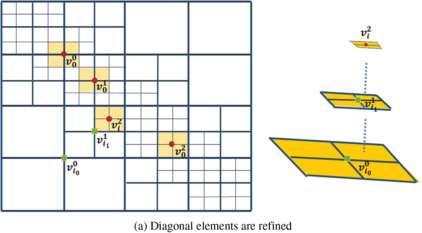
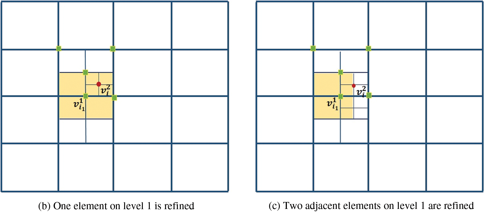
Figure 3: (a) The weights associated
• The weights of
• The weights for
Then, we obtain
• The non-vanishing basis functions at
Submitting
Fig. 3b shows a case where the weights for
The basis functions correspond to zero weights has no contribution in the entire representation. Notice that zero weights occur if and only if the function g form a partition of unity on the domain occupied by the support mesh of the considered basis vertex. Therefore, to avoid this, the isolated refined elements, like the case in Fig. 3b, are not allowed.
In Fig. 3c, two adjacent elements are refined. The support of
Based on the above analysis, we made the following assumptions for the hierarchical T-mesh to define positively weighted bases that form a partition of unity.
Definition 2 A hierarchical T-mesh is called an admissible hierarchical T-mesh if there are not any isolated refined elements in the hierarchical T-mesh. If an element on level
Figs. 3a and 3c are two admissible hierarchical T-meshes, while Fig. 3b is not an admissible hierarchical T-mesh. A hierarchical T-mesh can become an admissible hierarchical T-meshes by performing refinement on adjacent elements of isolated refined elements.
To ensure the refinement is highly localized, we generally require the refinement level between any two neighboring elements cannot be greater than one, which is also required in [18]. Under this requirement, hierarchical T-meshes are admissible.
Proposition 1 There uniquely exists a set of positive weights for the bases constructed in [2] on the admissible hierarchical T-mesh such that the weighted bases form a partition of unity, that is there uniquely exists
Proof The existence and uniqueness of the weights
For the basis functions
For an element
Since
then
This implies that the weights
because
In Fig. 4, we show the PHT surfaces defined over the same hierarchical T-mesh and by the same control points, but using different bases: the proposed weighted bases and non-decay bases [2]. The control points are designed on the plane
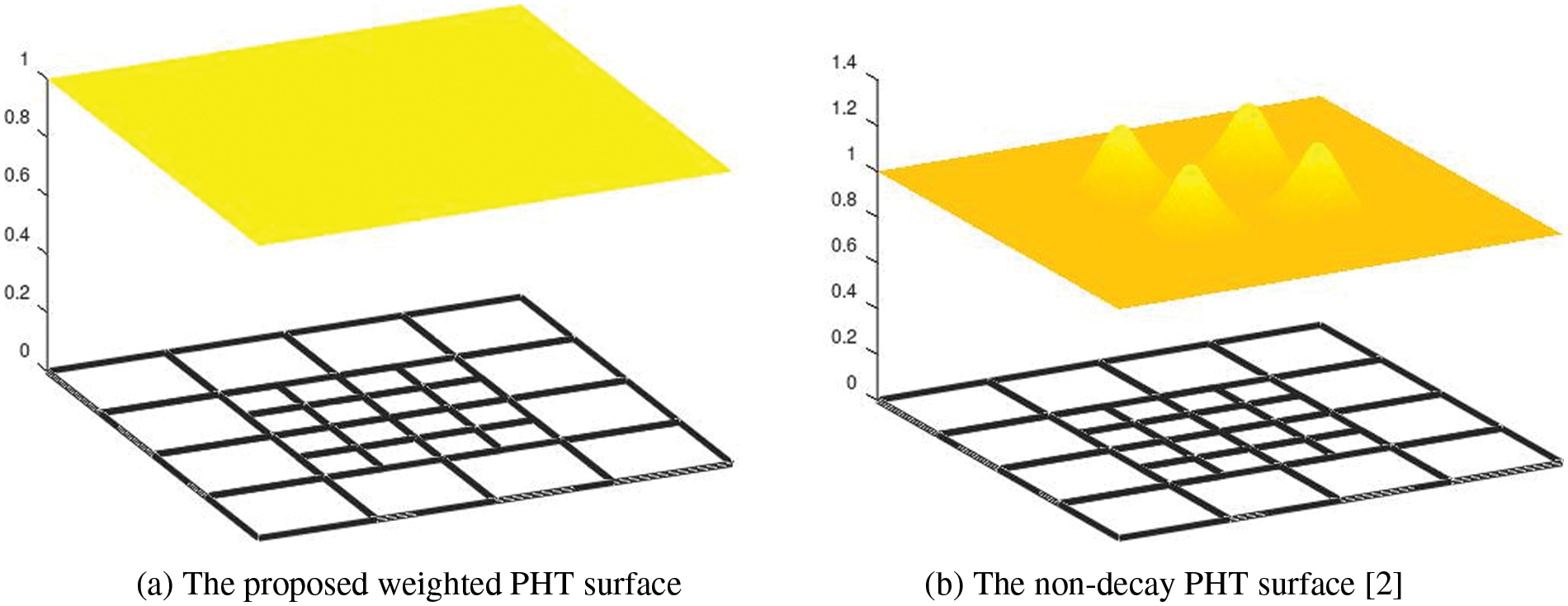
Figure 4: The weighted PHT-splines proposed in this paper form the partition of unity, while the PHT-splines defined by the non-decay bases [2] cannot form a partition of unity
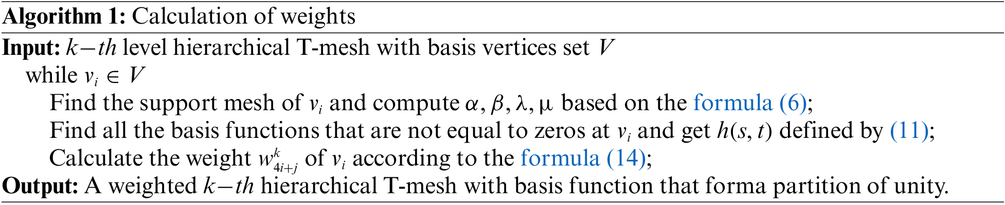
We conclude the method of computing the weights such that the weighted basis functions form a partition of unity in Algorithm 1.
4 Subdivision Scheme for PHT-Splines
Considering a knot vector
where
Based on the above formula, we derive the subdivision scheme for PHT-splines as follows. The support mesh of a basis vertex
• Vertex-points
If the refinement changes the support mesh associated with
where
Figure 5: Subdivision scheme of vertex points
• Edge-points
Suppose
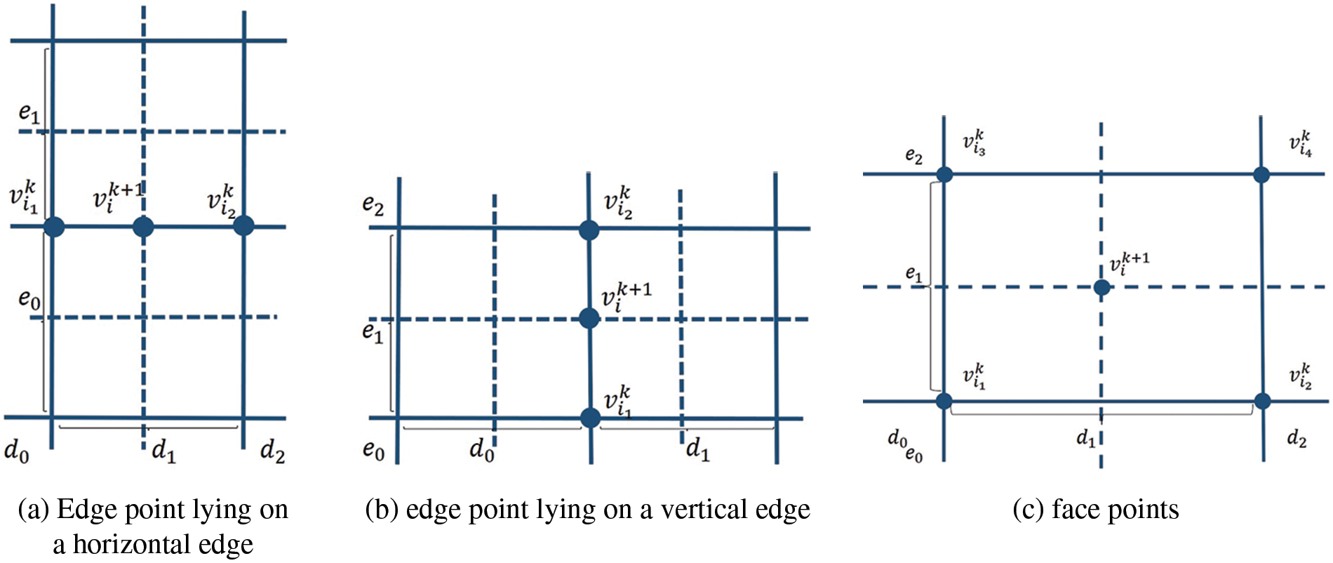
Figure 6: The subdivision scheme of edge points and face points
When the edge point lies on a vertical edge, as shown in Fig. 6b, the update formula is similar to the above one, except that
• Face-points
Since we assume the level difference in the mesh is not greater than 1, so when an element is refined, the four corners are exactly basis vertices. Suppose the four basis vertices of the refined face
The weights satisfying (9) can be computed by this subdivision scheme. The control points (weights) at level 0 are all set to be 1. In the following, we take the hierarchical T-mesh shown in Fig. 3a as an example to show how to use subdivision scheme to compute weights.
The weights are computed level by level. Fig. 7 shows the refinement process. The weights of the basis functions on level 0 are set as [1, 1, 1, 1], that is we set
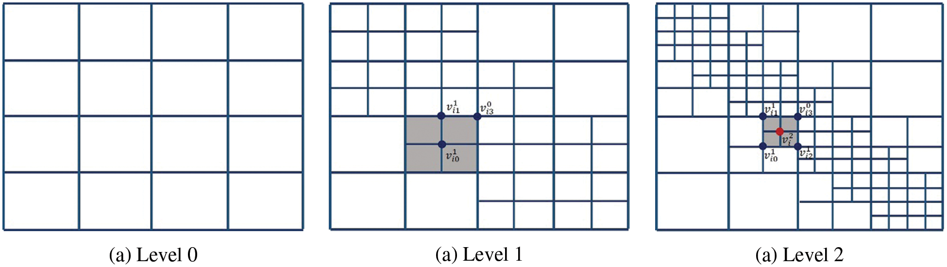
Figure 7: The weights of each level of mesh in Fig. 3a are calculated by the PHT-splines subdivision scheme
For the face point
For the vertex point
On level 2, the mesh is shown in Fig. 7c, the face points and edge points of level 1 now become vertex points. For example, the vertices marked by blue circles are vertex points and updated based on (20). Since all the support meshes of these vertices are not changed, their weights are equal to the weights computed on level 1. For the update of
For the face point
The weighted basis functions not only avoid the decay phenomenon, but also form a partition of unity. The non-decay property reduces the condition number of the stiffness matrix, thus gives better numerical stability. This advantage has been explored in [2] and will not be repeated in this paper. The focus of this paper is to provide a way to efficiently calculate weights for non-decay basis functions so that non-decay PHT splines can be used in specific applications, such as topology optimization [14].
In this section, three typical hierarchical T-meshes demonstrate the validity of the proposed methods. We see that the weights on admissible hierarchical T-meshes are all positive.
The hierarchical T-meshes here are produced in the context of iso-geometric analysis. The Poisson equation is defined as
The exact solution
The other two are smooth functions with large gradients at some local regions,
and
Fig. 8a shows the plot of
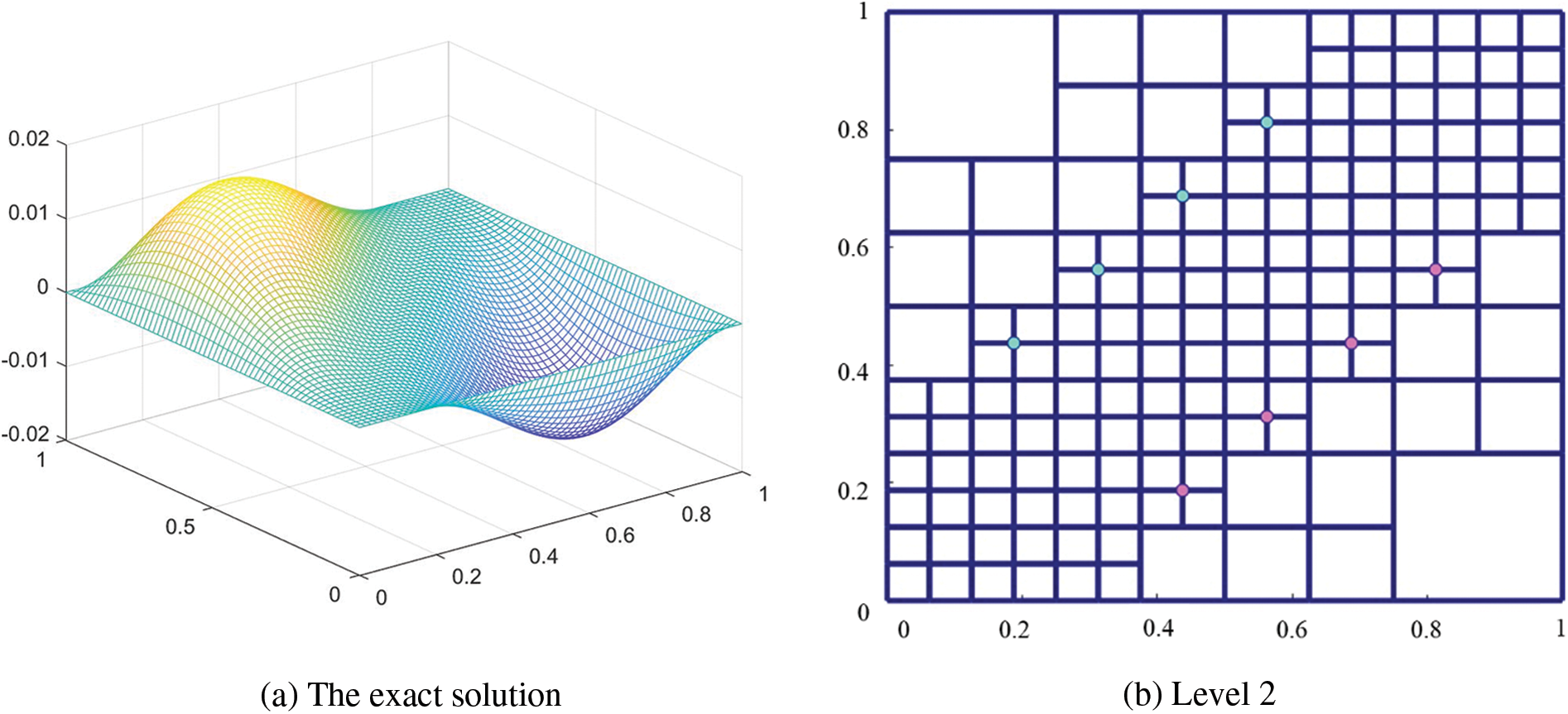
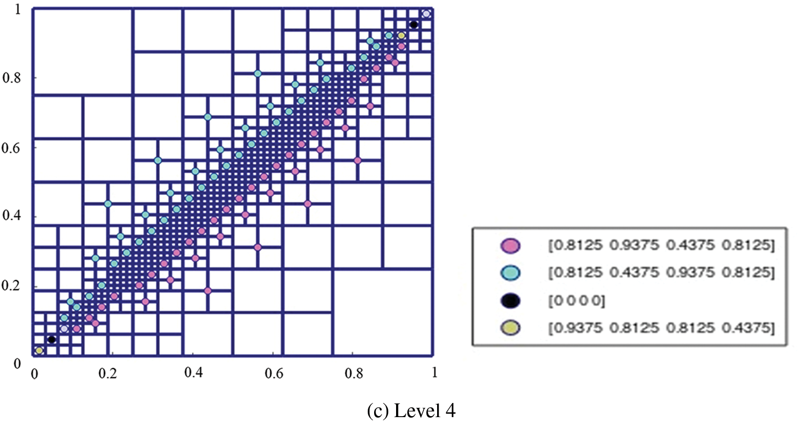
Figure 8: The weights of the basis functions on the hierarchical T-mesh with diagonal elements refined
Fig. 9a shows the plot of
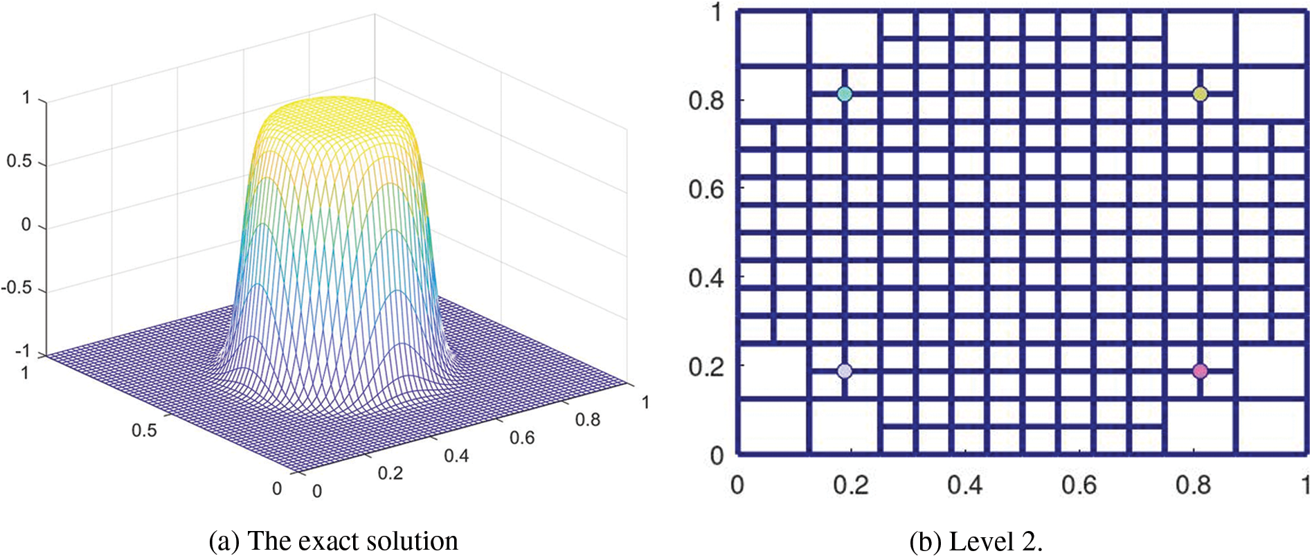
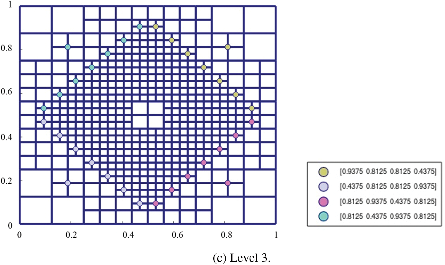
Figure 9: The weights of the basis functions on the hierarchical T-mesh solved from
Fig. 10a shows the plot of
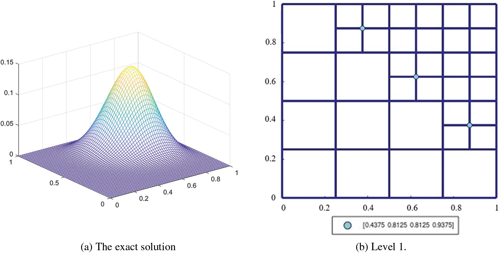
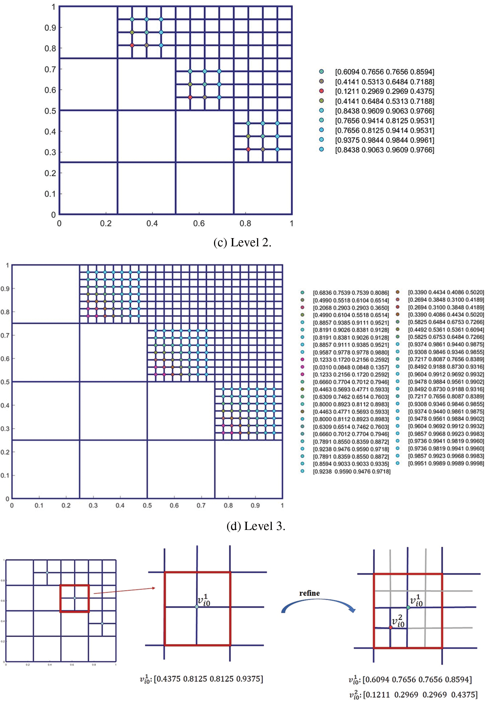
Figure 10: The weights of the basis functions on the hierarchical T-mesh solved from
In this paper, we proposed two efficient ways of computing weights for the PHT-splines basis functions constructed in [2] such that the weighted basis functions form a partition of unity. The weights are expressed explicitly based on the geometric information of related basis functions or by the subdivision formula of HT-splines. Both algorithms can effectively compute weights. We proved that the weights are positive on the admissible hierarchical T-meshes. Three typical hierarchical T-meshes are demonstrated to verify the effectiveness of the proposed methods.
There are several problems worthy of further discussion. The first one is to derive the subdivision scheme in the case of arbitrary level differences. Another issue worthy of exploring is the application of PHT-splines defined by a weighted basis in topology optimization and isogeometric collocation.
Acknowledgement: The authors thank the reviewers for providing useful comments and suggestion.
Funding Statement: The work was supported by the NSF of China (No. 11801393) and the Natural Science Foundation of Jiangsu Province, China (No. BK20180831).
Author Contributions: Falai Chen contributed to the conception of the study; Zhiguo Yong and Hongmei Kang contributed significantly to data analyses and manuscript writting; Zhiguo Yong performed the experiment.
Availability of Data and Materials: None.
Conflicts of Interest: The authors declare that they have no conflicts of interest to report regarding the present study.
References
1. Deng, J., Chen, F., Li, X., Hu, C., Tong, W. et al. (2008). Polynomial splines over hierarchical T-meshes. Graphical Models, 70(4), 76–86. [Google Scholar]
2. Kang, H., Xu, J., Chen, F., Deng, J. (2015). A new basis for PHT-splines. Graphical Models, 82, 149–159. [Google Scholar]
3. Li, X., Deng, J., Chen, F. (2007). Surface modeling with polynomial splines over hierarchical T-meshes. The Visual Computer, 23(12), 1027–1033. [Google Scholar]
4. Wang, J., Yang, Z., Jin, L., Deng, J., Chen, F. (2010). Adaptive surface reconstruction based on implicit PHT-splines. Proceedings of the 14th ACM Symposium on Solid and Physical Modeling, pp. 101–110. Haifa, Israel. [Google Scholar]
5. Tian, L., Chen, F., Du, Q. (2011). Adaptive finite element methods for elliptic equations over hierarchical T-meshes. Journal of Computational and Applied Mathematics, 236(5), 878–891. [Google Scholar]
6. Chan, C. L., Anitescu, C., Rabczuk, T. (2017). Volumetric parametrization from a level set boundary representation with PHT-splines. Computer-Aided Design, 82, 29–41. [Google Scholar]
7. Nguyen-Thanh, N., Kiendl, J., Nguyen-Xuan, H., W¨uchner, R., Bletzinger, K. U. et al. (2011). Rotation free isogeometric thin shell analysis using PHT-splines. Computer Methods in Applied Mechanics and Engineering, 200(47–48), 3410–3424. [Google Scholar]
8. Nguyen-Thanh, N., Muthu, J., Zhuang, X., Rabczuk, T. (2014). An adaptive three-dimensional RHT-splines formulation in linear elasto-statics and elasto-dynamics. Computational Mechanics, 53(2), 369–385. [Google Scholar]
9. Nguyen-Thanh, N., Nguyen-Xuan, H., Bordas, S. P. A., Rabczuk, T. (2011). Isogeometric analysis using polynomial splines over hierarchical T-meshes for two-dimensional elastic solids. Computer Methods in Applied Mechanics and Engineering, 200(21–22), 1892–1908. [Google Scholar]
10. Nguyen-Thanh, N., Zhou, K. (2017). Extended isogeometric analysis based on PHT-splines for crack propagation near inclusions. International Journal for Numerical Methods in Engineering, 112(12), 1777–1800. [Google Scholar]
11. Videla, J., Anitescu, C., Khajah, T., Bordas, S. P., Atroshchenko, E. (2019). h- and p-adaptivity driven by recovery and residual-based error estimators for PHT-splines applied to time-harmonic acoustics. Computers & Mathematics with Applications, 77(9), 2369–2395. [Google Scholar]
12. Wang, P., Xu, J., Deng, J., Chen, F. (2011). Adaptive isogeometric analysis using rational PHT-splines. Computer-Aided Design, 43(11), 1438–1448. [Google Scholar]
13. Yang, H., Dong, C. (2019). Adaptive extended isogeometric analysis based on PHT-splines for thin cracked plates and shells with Kirchhoff–Love theory. Applied Mathematical Modelling, 76, 759–799. [Google Scholar]
14. Gupta, A., Mamindlapelly, B., Karuthedath, P. L., Chowdhury, R., Chakrabarti, A. (2022). Adaptive isogeometric topology optimization using PHT splines. Computer Methods in Applied Mechanics and Engineering, 395, 114993. [Google Scholar]
15. Li, X., Deng, J., Chen, F. (2010). Polynomial splines over general T-meshes. The Visual Computer, 26(4), 277–286. [Google Scholar]
16. Ni, Q., Wang, X., Deng, J. (2019). Modified PHT-splines. Computer Aided Geometric Design, 73, 37–53. [Google Scholar]
17. Melenk, J. M., Babuška, I. (1996). The partition of unity finite element method: Basic theory and applications. Computer Methods Applied Mechanics Engineering, 139, 289–314. [Google Scholar]
18. Babuška, I., Melenk, J. M. (1997). The partition of unity method. International Journal for Numerical Methods in Engineering, 40, 727–758. [Google Scholar]
19. Pask, J. E., Sukumar, N. (2017). Partition of unity finite element method for quantum mechanical materials calculations. Extreme Mechanics Letters, 11, 8–17. [Google Scholar]
20. Giannelli, C., Juttler, B., Speleers, H. (2012). THB-splines: The truncated basis for hierarchical splines. Computer Aided Geometric Design, 29(7), 485–498. [Google Scholar]
21. Wei, X., Zhang, Y., Liu, L., Hughes, T. J. (2017). Truncated T-splines: Fundamentals and methods. Computer Methods in Applied Mechanics and Engineering, 316, 349–372. [Google Scholar]
22. Zhu, Y., Chen, F. (2017). Modified bases of PHT-splines. Communications in Mathematics and Statistics, 5(4), 381–397. [Google Scholar]
23. Deng, J., Chen, F., Feng, Y. (2006). Dimensions of spline spaces over T-meshes. Journal of Computational and Applied Mathematics, 194(2), 267–283. [Google Scholar]
Cite This Article
 Copyright © 2024 The Author(s). Published by Tech Science Press.
This work is licensed under a Creative Commons Attribution 4.0 International License , which permits unrestricted use, distribution, and reproduction in any medium, provided the original work is properly cited.
 Downloads
 Citation Tools