
 Submit a Paper
 Propose a Special lssue
 Open Access
ARTICLE
A New Scheme of the ARA Transform for Solving Fractional-Order Waves-Like Equations Involving Variable Coefficients
1 Department of Mathematics, Huzhou University, Huzhou, 313000, China
2 Department of Mathematics, Imam Mohammad Ibn Saud Islamic University, Riyadh, 11461, Saudi Arabia
3 Department of Basic Sciences and Humanities, UET Lahore, Faisalabad Campus, 54800, Pakistan
4 Department of Mathematics, Government College University, Faisalabad, 38000, Pakistan
5 Department of Mathematics and Statistics, College of Science, Taif University, P. O. Box 11099, Taif, 21944, Saudi Arabia
* Corresponding Author: Saima Rashid. Email:
(This article belongs to the Special Issue: On Innovative Ideas in Pure and Applied Mathematics with Applications)
Computer Modeling in Engineering & Sciences 2024, 138(1), 761-791. https://doi.org/10.32604/cmes.2023.028600
Received 27 December 2022; Accepted 19 April 2023; Issue published 22 September 2023
 View Full Text
 Download PDF
Abstract
The goal of this research is to develop a new, simplified analytical method known as the ARA-residue power series method for obtaining exact-approximate solutions employing Caputo type fractional partial differential equations (PDEs) with variable coefficient. ARA-transform is a robust and highly flexible generalization that unifies several existing transforms. The key concept behind this method is to create approximate series outcomes by implementing the ARA-transform and Taylor’s expansion. The process of finding approximations for dynamical fractional-order PDEs is challenging, but the ARA-residual power series technique magnifies this challenge by articulating the solution in a series pattern and then determining the series coefficients by employing the residual component and the limit at infinity concepts. This approach is effective and useful for solving a massive class of fractional-order PDEs. Five appealing implementations are taken into consideration to demonstrate the effectiveness of the projected technique in creating solitary series findings for the governing equations with variable coefficients. Additionally, several visualizations are drawn for different fractional-order values. Besides that, the estimated findings by the proposed technique are in close agreement with the exact outcomes. Finally, statistical analyses further validate the efficacy, dependability and steady interconnectivity of the suggested ARA-residue power series approach.Keywords
Several real-life occurrences in thermodynamics, molecular biology, operations research, and other disciplines of materials research can be lucratively modelled using fractional derivatives [1–6]. The principal motivation behind this is that realistic modelling of a core challenge requires not only the precise moment but also the preceding sequential schedule, which can be efficiently accomplished by utilizing fractional calculus [7,8]. However, numerous applied science researchers have concentrated on fractional partial differential equations (PDEs) in designing procedures for interaction problems and discussing physical phenomena. Aside from that, estimated and analytical strategies for FDE solutions have been investigated [9,10]. The subject of fractional initial value problems (IVPs) has captured the attention of academic researchers because it has the functionality of describing several capabilities of real-life manifestations within a more believable methodology than conventional PDEs. Many accomplishments have been attributed to the assumption of strategy presence and consistency in the fractional IVP framework [11]. For additional scientific articles on fractional ordinary and PDEs emerging in various fields of scientific research, see [12–14].
In a given situation, the level of flexibility of the nonlinear system in contemporary calculus (such as conventional calculus) is greater than that of the local differential equations operator. Authors [15,16] encompass the following applications of computation. As a consequence, intellectuals place an elevated significance on the investigation of non-integer order differentiation and integration. Geometrically, the arbitrarily defined order derivatives, which are predominantly predefined integrals, describe the complete function’s concentration, or the entire global integration variety [17,18]. The practise of academics has greatly boosted the efficiency of differential equations as well as quantitative and quantifiable scientific studies. It is worth noting that the following derivative operators were developed using conclusive essential methodologies. It is a well-established fact that there is currently no underlying solution to this problem. Consequently, the power law kernel has multiple interpretations. The Caputo fractional-order derivative (CFD) [19] is perhaps the most appealing underlying conceptualization. Dynamical formulae are notorious for being hard to address quantitatively or precisely. As a result, computational intelligence methodologies for evaluating the foregoing formulas have been constructed. Numerous intellectuals have mainly investigated computational perspectives to investigate fractional PDE under CFD [20,21].
Furthermore, owing to the quantitative intricacies of the fractional operators involved, figuring out the numerical method for fractional IVP processes can be occasionally challenging. In this context, computational and analytical strategies have been created and energized in order to explore the outcomes of various types of linear/nonlinear fractional IVP mechanisms. To reference a couple different ones: the Adomian decomposition method, Legendre polynomial, Lie symmetry analysis, Haar wavelet method, spectral collocation method, homotopy perturbation method, homotopy analysis transform method, reproducing kernel Hilbert space method, Bernoulli polynomials, B-spline functions, Chebyshev polynomials and the residue power series method, see [22–24].
In 2013, Omar Abu Arqub, a Jordanian mathematician [25], invented the residual power series method (RPSM). However, RPSM is an analytical procedure for tackling ordinary, partial, and fuzzy DEs, as well as fractional-order integro-DEs, which correlates with the Taylor’s series having the residual error function. It offers linear and nonlinear DE series strategies in the context of convergence series. For its inaugural moment, RPSM was used to develop solutions to fuzzy DEs in 2013. Arqub et al. [26] applied an efficient technique for addressing the solution of higher-order IVP. Arqub et al. [27] used the RPSM to consider numerous findings for dynamical fractional-order boundary value problems. El-Ajou et al. [28] expounded the novel recursive approach RPSM for establishing the solutions of the nonlinear fractional KdV-Burgers model. Later on, this dynamical scheme merged with several integral transforms to make it more comprehensive. It is a useful meta-heuristic algorithm because it applies with the help of closed-form functional information. In the scenario of nonlinear challenges, obtaining a solution in closed form is unattainable, and determining the series coefficients is a tough challenge. To address the shortcomings of the classic PSM, an optimized version of the PSM is introduced that treats the coefficient values as transmogrified operations that pursue a set of regulations and are ascertained by recurrence connections. For more details on RPSM, see [29–31].
In 1780, the French mathematician and physicist P. S. Laplace [32,33] proposed the integral transform. In 1822, J. Fourier [34] invented the Fourier transform. Laplace and Fourier transforms are the cornerstone of operations and maintenance interpretation, a strand of mathematical concepts with enormously potent implementations not just in mathematical modeling but also in different scientific fields such as thermodynamics, technology, cosmology, and so forth. This research is based on the implementation of the ARA Ts (ARA Ts), an innovative integral transform, introduced by Saadeh et al. [35]. This transform is an influential and multi-functional generalization that consolidates several configurations of the conventional Laplace transform, including the Sumudu transform [36], the Elzaki transform [37], the Natural transform [38], the Yang transform [39] and the Shehu transform [40].
Numerous publications have been written to explain dynamic processes that can be induced and propagated in a variety of concentrations and configurations. The majority of academics have concentrated on minimizing the fundamental formulae of varying concentration models to evolution problems in the pattern of PDES such as the Swift-Hohenberg model (KdV) equation, Burger equation, Black-Scholes model, Boussinesq equation and so on [41–44].
Another development of the RPSM is assembled in this article by acclimating the ARA Ts [35,45] to the RPSM technique [25,26]. In this article, the new framework, ARA-residual power series method (ARARPSM), is used to effectively resolve fractional-order PDEs. Furthermore, the detailed explanation of the nonlinear fractional-order PDEs is outlined below:
• The ARARPSM is an efficacious approach and a novel method for obtaining numerical approximations to dynamical fractional PDEs in series pattern. The series coefficients can be ascertained quickly by employing the notion of limit at
• Five problems are analyzed statistically to identify the reliability and robustness of the suggested technique. Furthermore, analytical findings are also compared with the existing results and are in agreement with the exact findings and several other techniques.
• Diagrammatically, relevance is indeed discovered for multiple fractional-order derivative attributes and the statistical performances of the mean absolute deviation, mean deviation, Theil’s inequality coefficients, and semi-interquartile range. Hence, the methodology is accurate, easy to employ, not influenced by supercomputing iterations of inconsistencies, and doesn’t necessitate an enormous amount of memory storage or time.
• This technique, unlike the conventional power series technique, somehow doesn’t entail identifying the coefficient values of the commensurate terms or the application of a recursion connection. The suggested restriction concept-based methodology shows series coefficients but not fractional derivatives, similar to the RPSM. Unlike RPSM, which also demands numerous computations to quantify multiple fractional derivatives during the completion of the task successfully, only a very few computations are required to evaluate the coefficients.
This section provides a number of interpretations, characteristics, and some helpful findings that form the foundation of the novel methodology. The ARA Ts is derived using the classic Laplace integral. In order to simplify the method for solving ordinary and partial DEs in the temporal domain, Saadeh et al. [35] proposed the ARA Ts in 2020. ARA is the identifier of the proposed transform; the term is not an acronym. It has some interesting properties, such as the ability to generate multiple transforms by varying the significance of the index
Definition 2.1. ([22]) For
where
Definition 2.2. ([35]) The ARA Ts of order
In the assertions that follow, we list a few ARA Ts ation fundamentals [35] that are crucial to our studies.
Suppose that there are two continuous mappings
(i)
(ii)
(iii)
(iv)
(v)
(vi)
(vii)
Theorem 2.3. ([25]) Assume there is a mapping
For continuous mappings
where
Theorem 2.4. ([46]) Suppose there is a continuous mapping
Then
Remark 1. (a) The
(b) For the ARA Ts of order two of the mapping
and the
(c) The inverse of the ARA Ts of order two for the FPS (1) is presented as follows:
Theorem 2.5. ([46]) Assume that there is a continuous mapping
where
If
3 Configuring Series Findings of FPDEs
In this section, the new framework, ARARPSM, is used to effectively resolve fractional-order PDEs of the form:
subject to the initial settings
where
This part explains the ARA-RPS approach to addressing time-fractional PDEs. The proposed method relies on Taylor’s expansion to generate solitary solutions after applying the ARA Ts to the governing formulation.
Taking the initial value problem (IVP) (7) and (8), we implement the ARARPSM.
Apply the ARA Ts of order two
In view of assertion (vi) and the initial conditions (8), then (9) reduces to
Suppose that the respective series conceptions correspond to the ARA-RPS solution of formula (9) has the following form:
and
Making the use of assertion (vii), we have
Since
To obtain
or accordingly
Now, assertion (v) provides that
Employing assertion (iv), we attain
Assertions (ii) and (vii) lead to
Therefore, the ARA-RPS findings of (10) has the series formulations:
and the
To determine the parameter estimates of series developments in (17) and (18), we describe the ARA-residual component of (10), as shown
and the truncated
Multiplying both sides of (18) by
The ARA-RPS solution can be found by releasing the evidence below:
In order to achieve the solution of the IVP (7) and (8) in the feature space, the achieved coefficients
Here, we take into consideration three well-known and significant time fractional PDEs with varying coefficients challenges in order to illustrate the effectiveness and appropriateness of ARARPSM.
Example 1. Assume the subsequent nonlinear time fractional
where
Proof. Implementing the ARA Ts of order two
It follows that
After simplification, (24) reduces to
Suppose that the ARA-RPS result of (25) has the subsequent series expression:
and the
Conducting product both sides of (29) by
In view of the following assumption, we have
and the initial settings mentioned in (22), we deduce that
In order to evaluate
Therefore, we have
It follows that
Considering assertion (v) provides that
Making the use of assertion (iv), gives
Making the use of assertion (ii) and (vii) lead us
Therefore, the ARA-RPS findings of (25) has the subsequent series formulations:
and the
Furthermore, we classify the ARA-residue function of (25), then
and the
Utilizing the fact that
In order to evaluate the second unknown coefficient
Plugging
in (38) and simple computations yield
where
Revisiting the analogous process, we can evaluate the coefficients of the series (26) as follows:
Hence, the seventh approximate solution of (26) is
Applying the inverse ARA Ts
For integer-order solution, the approximated solution (39) reduces to
It is worth noting that the integer-order solution (40) coincides with the result proposed by Khalouta et al. [47].
Example 2. Assume the subsequent nonlinear time fractional wave-like equation [47]:
where
Proof. Implementing the ARA Ts of order two
It follows that
After simplification, (44) reduces to
Suppose that the ARA-RPS result of (45) has the subsequent series expression:
Here, the expansions in (46)
Introducing the
Conducting product on both sides of (48) by
Plugging the coefficients in the series expansion of
Using the inverse ARA Ts of order two
For integer-order solution, the approximated solution of (50) reduces to
It is worth noting that the integer-order solution (51) coincides with the result proposed by Khalouta et al. [47].
Example 3. Assume the subsequent nonlinear time-fractional
where
Proof. Implementing the ARA Ts of order two
It follows that
After simplification, (55) reduces to
Suppose that the ARA-RPS result of (56) has the subsequent series expression:
Here, the expansions in (57)
Introducing the
Conducting product on both sides of (59) by
Plugging the coefficients in the series expansion of
Using the inverse ARA Ts of order two
For integer-order solution, the approximated solution of (61) reduces to
It is worth noting that the integer-order solution (62) coincides with the result proposed by Khan et al. [48].
Example 4. Assume the subsequent nonlinear time-fractional
where
Proof. Implementing the ARA Ts of order two
It follows that
After simplification, (66) reduces to
Suppose that the ARA-RPS result of (67) has the subsequent series expression:
Here, the expansions in (68)
Introducing the
Conducting product on both sides of (70) by
Plugging the coefficients in the series expansion of
Using the inverse ARA Ts of order two
For integer-order solution, the approximated solution of (72) reduces to
It is worth noting that the integer-order solution (73) coincides with the result proposed by [48,49].
Example 5. Assume the subsequent 2D nonlinear time-fractional wave-like equation [47]:
where
Proof. Implementing the ARA Ts of order two
It follows that
After simplification, (77) reduces to
Suppose that the ARA-RPS result of (78) has the subsequent series expression:
Here, the expansions in (79)
Introducing the
Conducting product on both sides of (81) by
Plugging the coefficients in the series expansion of
Using the inverse ARA Ts of order two
For integer-order solution, the approximated solution of (83) reduces to
It is worth noting that the integer-order solution (84) coincides with the result proposed by Khalouta et al. [47].
5 Numerical Simulation and Performance Techniques
Here, the consequences of the approximate and exact solutions to the approaches presented in Examples 1–5 are evaluated graphically and numerically in this portion. In the context of an infinite fractional power series, it is critical to supply the approximation inconsistencies of the estimated solution provided by ARARPSM. To illustrate the precision and competence of ARARPSM, we used the residual, mean absolute deviation (MAD):
The approximate results produced using the suggested procedure and the accurate solving Examples 1–5 are compared in Figs. 1–5a via a two-dimensional plot. From Figs. 1–5a, it can be seen that the analytical seventh-order solutions at

Figure 1: Graphical illustrations for Example 1. (a) Two-dimensional plots for various values of fractional-order in comparison with the exact solution. (b) Histogram plots on the mean, mean-deviation, semi-interquartile range and standard deviation

Figure 2: Graphical illustrations for Example 2. (a) Two-dimensional plots for various values of fractional-order in comparison with the exact solution. (b) Histogram plots on the mean, mean-deviation, semi-interquartile range and standard deviation

Figure 3: Graphical illustrations for Example 3. (a) Two-dimensional plots for various values of fractional-order in comparison with the exact solution. (b) Histogram plots on the mean, mean-deviation, semi-interquartile range and standard deviation

Figure 4: Graphical illustrations for Example 4. (a) Two-dimensional plots for various values of fractional-order in comparison with the exact solution. (b) Histogram plots on the mean, mean-deviation, semi-interquartile range and standard deviation

Figure 5: Graphical illustrations for Example 5. (a) Two-dimensional plots for various values of fractional-order in comparison with the exact solution. (b) Histogram plots on the mean, mean-deviation, semi-interquartile range and standard deviation
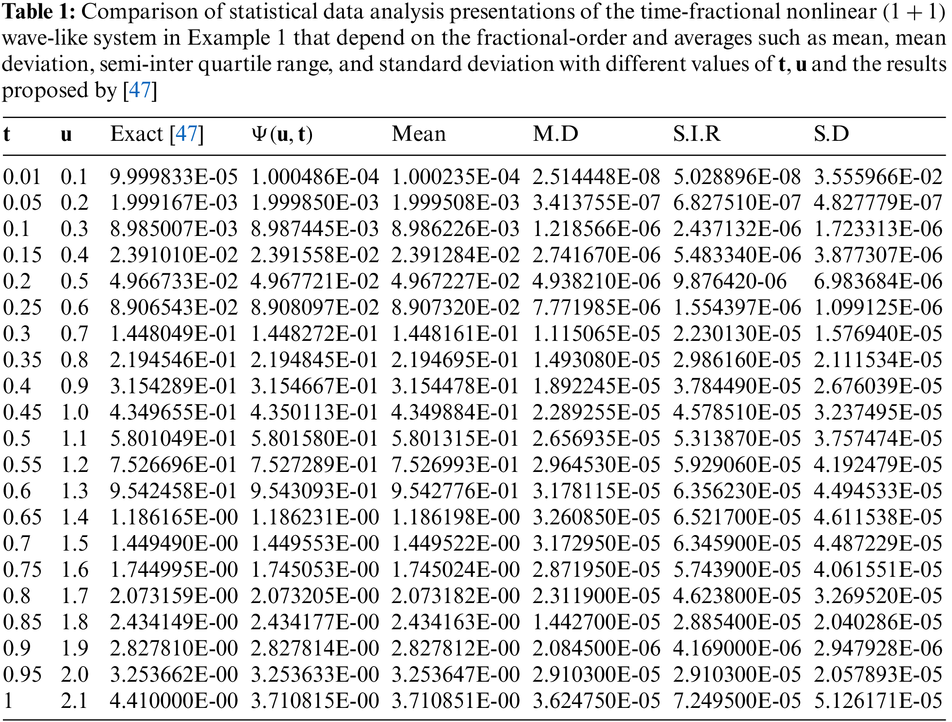


Figs. 1–5b show the visual display of the statistical efficiency interventions along with their analysis on histograms for the results of the ARARPSM for the proposed dynamical systems. However, the ideal outcomes are depicted by exact and approximated values are discovered around

The accuracy, exactness, and efficacy of the interconnected supercomputing algorithms of ARARPSMA for tackling the nonlinear wave-likeand heat-like systems are further indicated by standard measures such as G-TIC, G-MAD, and G-EVAF that are similar to their optimal setting.
Eventually, the major aspects of the ARA-PSM are as follows, as shown by the numerical, graphically and statistical outcomes: The suggested approach is a methodical, potent, and essential component for fractional-order PDEs estimated and exact solutions. The resilience of the mechanism lies in the fact that the presented strategy requires very few estimations than established computational models and is therefore more precise and cost-effective. In comparison to the variational iteration mechanism and the Adomian decomposition technique, the envisaged technique has the opportunity that it can help address computational complexity avoiding the He’s polynomials or Adomian polynomials. The proposed method is founded on a latest iteration of Taylor’s series that yields a convergent series as a solution. When determining the coefficient values for a succession such as the RPSM, the fractional derivatives must be calculated every time. We only require to perform a handful calculations to obtain the coefficients because ARARPSM only necessitates the idea of an infinite threshold. The relatively high level of exactness has been affirmed by the statistical analysis. To lesser estimations and iterative process actions, we came to the conclusion that the envisaged methodology is a practical and effective approach for tackling some categories of fractional-order PDEs.
In this paper, we presented a novel methodology for addressing fractional-order PDEs with variable coefficients in the context of a Caputo fractional derivative employing the ARA Ts and RPSM. Using the ARARPSM, we were able to address several dynamical fractional PDEs as well as illustrate a novel algorithm regarding them. Statistical or mathematical outcomes serve as evidence of the ARARPSM’s effectiveness. Complex nonlinear systems’ objective measurements for Examples 1–5 statistical data analysis comparison have been provided in Table 6, which shows how the measure of dispersion has a significant impact on the proposed findings. These graphs and tables show that the ARARPSM’s approximations and the corresponding exact solutions are in good accordance with each other. Additionally, the MAD, TIC and EVAF formulation significance levels confirm the effectiveness of tackling the multidimensional fractional-order PDEs. Its accuracy and value are verified by assertions made utilizing statistical identifiers for various independent implementations employing the suggested ARARPSM predicted on the mean, mean deviation, S.I.R and S.D infiltrators. The error estimates for the projected framework range from

Acknowledgement: The researchers would like to acknowledge the Deanship of Scientific Research, Taif University for funding this work.
Funding Statement: The authors received no specific funding for this study.
Author Contributions: All authors read and approved the final manuscript.
Availability of Data and Materials: No data were used to support this study.
Conflicts of Interest: The authors declare that they have no conflicts of interest to report regarding the present study.
References
1. Zheng, X., Wang, H. (2020). An optimal-order numerical approximation to variable-order space-fractional diffusion equations on uniform or graded meshes. SIAM Journal on Numerical Analysis, 58(1), 330–352. https://doi.org/10.1137/19M1245621 [Google Scholar] [CrossRef]
2. Zheng, X., Wang, H. (2020). An error estimate of a numerical approximation to a hidden-memory variable-order space-time fractional diffusion equation. SIAM Journal on Numerical Analysis, 58(5), 2492–2514. https://doi.org/10.1137/20M132420X [Google Scholar] [CrossRef]
3. Celikten, G. (2022). A logarithmic finite difference method for numerical solutions of the generalized huxley equation. Turkish Journal of Science, 7(1), 1–6. [Google Scholar]
4. Maitama, S., Zhao, W. (2019). New integral transform: Shehu transform a generalization of Sumudu and Laplace transform for solving differential equations. International Journal of Analysis and Applications, 17(2), 167–190. [Google Scholar]
5. Magin, R. L. (2006). Fractional calculus in bioengineering. Redding, CT, USA: Begell House Publishers. [Google Scholar]
6. Rihan, F. A. (2013). Numerical modeling of fractional-order biological systems. Abstract and Applied Analysis, 2013(2), 816803. https://doi.org/10.1155/2013/816803 [Google Scholar] [CrossRef]
7. Latha, V. P., Rihan, F. A., Rakkiyappan, R., Velmurugan, G. (2018). A fractional-order model for Ebola virus infection with delayed immune response on heterogeneous complex networks. Journal of Computation and Applied Mathematics, 339, 134–146. https://doi.org/10.1016/j.cam.2017.11.032 [Google Scholar] [CrossRef]
8. Thabet, S. T. M., Abdo, M. S., Shah, K., Abdeljawad, T. (2020). Study of transmission dynamics of COVID-19 mathematical model under ABC fractional order derivative. Results in Physics, 19(11), 103507. https://doi.org/10.1016/j.rinp.2020.103507 [Google Scholar] [PubMed] [CrossRef]
9. Atangana, A. (2020). Extension of rate of change concept: From local to nonlocal operators with applications. Results in Physics, 19(5), 103515. https://doi.org/10.1016/j.rinp.2020.103515 [Google Scholar] [CrossRef]
10. Gao, W., Veeresha, P., Baskonus, H. M., Prakasha, D. G., Kumar, P. (2020). A new study of unreported cases of 2019-nCOV epidemic outbreaks. Chaos Solitons and Fractals, 138(554), 109929. https://doi.org/10.1016/j.chaos.2020.109929 [Google Scholar] [PubMed] [CrossRef]
11. Shah, K., Abdeljawad, T., Alrabaiah, H. (2022). On coupled system of drug therapy via piecewise equations. Fractals, 30(8), 2240206. https://doi.org/10.1142/S0218348X2240206X [Google Scholar] [CrossRef]
12. Shah, K., Ahmad, I., Nieto, J. J., Rahman, G. U., Abdeljawad, T. (2022). Qualitative investigation of nonlinear fractional coupled pantograph impulsive differential equations. Qualitative Theory of Dynamical Systems, 21(4), 131. https://doi.org/10.1007/s12346-022-00665-z [Google Scholar] [CrossRef]
13. Heydari, M. H., Razzaghi, M. (2021). A numerical approach for a class of nonlinear optimal control problems with piecewise fractional derivative. Chaos Solitons and Fractals, 152(9–10), 111465. https://doi.org/10.1016/j.chaos.2021.111465 [Google Scholar] [CrossRef]
14. Heydari, M. H., Razzaghi, M., Baleanu, D. (2022). Orthonormal piecewise Vieta-Lucas functions for the numerical solution of the one- and two-dimensional piecewise fractional Galilei invariant advection-diffusion equations. Journal of Advance Research, 49, 175–190. https://doi.org/10.1016/j.jare.2022.10.002 [Google Scholar] [PubMed] [CrossRef]
15. Zhang, Y. -Z., Yang, A. -M., Long, Y. (2014). Initial boundary value problem for fractal heat equation in the semi-infinite region by Yang-Laplace transform. Thermal Science, 18(2), 677–681. [Google Scholar]
16. Rashid, S., Khalid, A., Sultana, S., Jarad, F., Abulanaja, K. M. et al. (2022). Novel numerical investigation of the fractional oncolytic effectiveness model with M1 virus via generalized fractional derivative with optimal criterion. Results in Physics, 37(42), 105553. https://doi.org/10.1016/j.rinp.2022.105553 [Google Scholar] [CrossRef]
17. Arqub, O. A., El-Ajou, A., Momani, S. (2015). Constructing and predicting solitary pattern solutions for nonlinear time-fractional dispersive partial differential equations. Journal of Computational Physics, 293, 385–399. https://doi.org/10.1016/j.jcp.2014.09.034 [Google Scholar] [CrossRef]
18. Atangana, A., Baleanu, D. (2016). New fractional derivatives with non-local and non-singular kernel: Theory and application to heat transfer model. Thermal Science, 20(2), 763–785. https://doi.org/10.2298/TSCI160111018A [Google Scholar] [CrossRef]
19. Alyousef, H. A., Salas, A. H., Matoog, R. T., El-Tantawy, S. A. (2022). On the analytical and numerical approximations to the forced damped Gardner Kawahara equation and modeling the nonlinear structures in a collisional plasma. Physics of Fluids, 34(10), 103105. https://doi.org/10.1063/5.0109427 [Google Scholar] [CrossRef]
20. Hilfer, R. (2000). Applications of fractional calculus in physics. Singapore: Word Scientific. [Google Scholar]
21. Kilbas, A., Srivastava, H. M., Trujillo, J. J. (2006). Theory and application of fractional differential equations. North Holland: Math Stud. [Google Scholar]
22. Podlubny, I. (1999). Fractional differential equations. San Diego: Academic Press. [Google Scholar]
23. Elbeleze, A. A., Kiliçman, A., Taib, B. M. (2014). Note on the convergence analysis of homotopy perturbation method for fractional partial differential equations. Abstract and Applied, 2014, 803902. https://doi.org/10.1155/2014/803902 [Google Scholar] [CrossRef]
24. Oderinu, R. A., Owolabi, J. A., Taiwo, M. (2023). Approximate solutions of linear time-fractional differential equations. Journal of Mathematics and Computer Science, 29(1), 60–72. [Google Scholar]
25. Senthilkumar, L. S., Mahendran, R., Subburayan, V. (2022). A second order convergent initial value method for singularly perturbed system of differential-difference equations of convection diffusion type. Journal of Mathematics and Computer Science, 25(1), 73–83. [Google Scholar]
26. Arqub, O. A., Abo-Hammour, Z., Al-Badarneh, R., Momani, S. (2013). A reliable analytical method for solving higher-order initial value problems. Discrete Dynamics in Nature and Society, 2013(29–32), 673829. https://doi.org/10.1155/2013/673829 [Google Scholar] [CrossRef]
27. Arqub, O. A., El-Ajou, A., Al Zhour, Z., Momani, S. (2014). Multiple solutions of nonlinear boundary value problems of fractional order: A new analytic iterative technique. Entropy, 16(1), 471–493. https://doi.org/10.3390/e16010471 [Google Scholar] [CrossRef]
28. El-Ajou, A., Arqub, O. A., Momani, S. (2015). Approximate analytical solution of the nonlinear fractional KdV-Burgers equation: A new iterative algorithm. Journal of Computational Physics, 293, 81–95. https://doi.org/10.1016/j.jcp.2014.08.004 [Google Scholar] [CrossRef]
29. Liaqat, M. I., Etemad, S., Rezapour, S., Park, C. (2022). A novel analytical Aboodh residual power series method for solving linear and nonlinear time-fractional partial differential equations with variable coefficients. AIMS Mathematics, 7(9), 16917–16948. https://doi.org/10.3934/math.2022929 [Google Scholar] [CrossRef]
30. Zhang, J., Wei, Z., Li, L., Zhou, C. (2019). Least-squares residual power series method for the time-fractional differential equations. Complexity, 2019, 6159024. https://doi.org/10.1155/2019/6159024 [Google Scholar] [CrossRef]
31. Jaradat, I., Alquran, M., Abdel-Muhsen, R. (2018). An analytical framework of 2D diffusion, wave-like, telegraph, and Burgers models with twofold Caputo derivatives ordering. Nonlinear Dynamics, 93(4), 1911–1922. https://doi.org/10.1007/s11071-018-4297-8 [Google Scholar] [CrossRef]
32. Widder, D. V. (1946). The laplace transform. London, UK: Princeton University Press. [Google Scholar]
33. Spiegel, M. R. (1965). Theory and problems of laplace transforms; Schaums outline series. New York, NY, USA: McGraw-Hill. [Google Scholar]
34. Bochner, S., Chandrasekharan, K. (1949). Fourier transforms. London, UK: Princeton University Press. [Google Scholar]
35. Saadeh, R., Qazza, A., Burqan, A. (2020). A new integral transform: ARA transform and its properties and applications. Symmetry, 12(6), 925. https://doi.org/10.3390/sym12060925 [Google Scholar] [CrossRef]
36. Watugula, G. K. (1993). Sumudu transform: A new integral transform to solve differential equations and control engineering problems. International Journal of Mathematical Education in Science and Technology, 24(1), 35–43. https://doi.org/10.1080/0020739930240105 [Google Scholar] [CrossRef]
37. Elzaki, T. M. (2011). The new integral transform Elzaki transform. Global Journal of Pure and Applied Mathematics, 7(1), 57–64. [Google Scholar]
38. Khan, Z. H., Khan, W. A. (2008). Natural transform-properties and applications. NUST Journal of Engineering Sciences, 1(1), 127–133. [Google Scholar]
39. Yang, X. J. (2016). A new integral transform with an application in heat transfer. Thermal Science, 20(3), 677–681. https://doi.org/10.2298/TSCI16S3677Y [Google Scholar] [CrossRef]
40. Maitama, S., Zhao, W. (2019). New integral transform: Shehu transform a generalization of Sumudu and Laplace transform for solving differential equations. International Journal of Analysis and Application, 17(2), 167–190. [Google Scholar]
41. Rashid, S., Sultana, S., Kanwal, B., Jarad, F., Khalid, A. (2022). Fuzzy fractional estimates of Swift-Hohenberg model pertaining to Atangana-Baleanu fractional derivative operator. AIMS Mathematics, 7(9), 16067–16101. https://doi.org/10.3934/math.2022880 [Google Scholar] [CrossRef]
42. Rashid, S., Sultana, S., Idrees, N., Bonyah, E. (2022). On analytical treatment for the fractional-order coupled partial differential equations via fixed point formulation and generalized fractional derivative operators. Journal of Function Spaces, 2022(2), 3764703. https://doi.org/10.1155/2022/3764703 [Google Scholar] [CrossRef]
43. Rashid, S., Butt, S. I., Hammouch, Z., Bonyah, E. (2022). An efficient method for solving fractional black-scholes model with index and exponential decay kernels. Journal of Function Spaces, 2022(1), 2613133. https://doi.org/10.1155/2022/2613133 [Google Scholar] [CrossRef]
44. Rashid S., Kaabar M. K. A., Althobaiti A., Alqurashi M. S. (2022). Constructing analytical estimates of the fuzzy fractional-order Boussinesq model and their application in oceanography. Journal of Ocean Engineering and Science, 8(2), 196–225. https://doi.org/10.1016/j.joes.2022.01.003 [Google Scholar] [CrossRef]
45. Qazza, A., Burqan, A., Saadeh, R. (2021). A new attractive method in solving families of fractional differential equations by a new transform. Mathematics, 9(23), 3039. https://doi.org/10.3390/math9233039 [Google Scholar] [CrossRef]
46. Burqan, A., Saadeh, R., Qazza, A. (2022). A novel numerical approach in solving fractional neutral pantograph equations via the ARA integral transform. Symmetry, 14(1), 50. https://doi.org/10.3390/sym14010050 [Google Scholar] [CrossRef]
47. Khalouta, A., Kadem, A. (2020). A new computational for approximate analytical solutions of nonlinear time-fractional wave-like equations with variable coefficients. AIMS Mathematics, 5(1), 1–14. https://doi.org/10.3934/math.2020001 [Google Scholar] [CrossRef]
48. Khan, H., Shah, R., Kumam, P., Arif, M. (2019). Analytical solutions of fractional-order heat and wave equations by the natural transform decomposition method. Entropy, 21(6), 597. https://doi.org/10.3390/e21060597 [Google Scholar] [PubMed] [CrossRef]
49. Chen, B., Qin, L., Xu, F., Zu, J. (2018). Applications of general residual power series method to differential equations with variable coefficients. Discrete Dynamics of Nonlinear Systems in Nature and Society, 2018, 2394735. https://doi.org/10.1155/2018/2394735 [Google Scholar] [CrossRef]
50. Chu, Y. M., Nazir, U., Sohail, M., Selim, M. M., Lee, J. R. (2021). Enhancement in thermal energy and solute particles using hybrid nanoparticles by engaging activation energy and chemical reaction over a parabolic surface via finite element approach. Fractal Fractional, 5(3), 119. https://doi.org/10.3390/fractalfract5030119 [Google Scholar] [CrossRef]
Cite This Article
 Copyright © 2024 The Author(s). Published by Tech Science Press.
This work is licensed under a Creative Commons Attribution 4.0 International License , which permits unrestricted use, distribution, and reproduction in any medium, provided the original work is properly cited.
 Downloads
 Citation Tools