
 Submit a Paper
 Propose a Special lssue
 Open Access
ARTICLE
Mixed Integer Robust Programming Model for Multimodal Fresh Agricultural Products Terminal Distribution Network Design
1 Business School, University of Shanghai for Science and Technology, Shanghai, 200093, China
2 School of Management, Shanghai University of International Business and Economics, Shanghai, 201620, China
* Corresponding Author: Zhong Wu. Email:
(This article belongs to the Special Issue: Data-Driven Robust Group Decision-Making Optimization and Application)
Computer Modeling in Engineering & Sciences 2024, 138(1), 719-738. https://doi.org/10.32604/cmes.2023.028699
Received 03 January 2023; Accepted 03 April 2023; Issue published 22 September 2023
 View Full Text
 Download PDF
Abstract
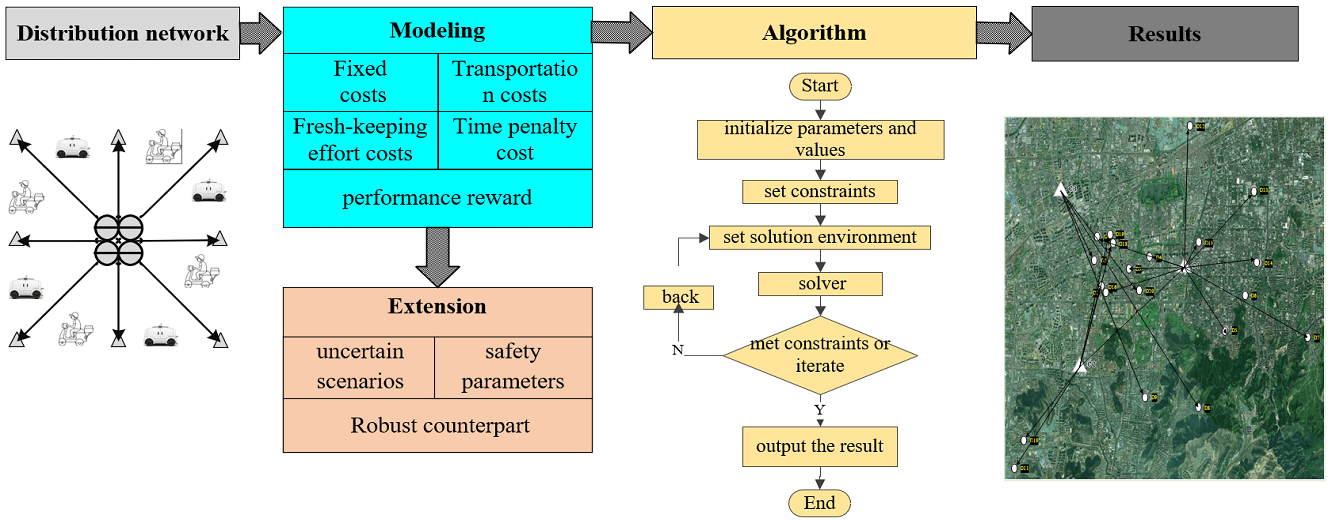
The low efficiency and high cost of fresh agricultural product terminal distribution directly restrict the operation of the entire supply network. To reduce costs and optimize the distribution network, we construct a mixed integer programming model that comprehensively considers to minimize fixed, transportation, fresh-keeping, time, carbon emissions, and performance incentive costs. We analyzed the performance of traditional rider distribution and robot distribution modes in detail. In addition, the uncertainty of the actual market demand poses a huge threat to the stability of the terminal distribution network. In order to resist uncertain interference, we further extend the model to a robust counterpart form. The results of the simulation show that the instability of random parameters will lead to an increase in the cost. Compared with the traditional rider distribution mode, the robot distribution mode can save 12.7% on logistics costs, and the distribution efficiency is higher. Our research can provide support for the design of planning schemes for transportation enterprise managers.Graphic Abstract
Keywords
Nomenclature
| Sets | |
| The set of distribution center node | |
| The set of demand node | |
| The set of positive integers | |
| Complete set | |
| The set of arcs | |
| The set of interval value uncertainty | |
| Parameter | |
| The costs of vehicle acquisition | |
| The costs of vehicle maintenance | |
| Unit energy cost of vehicle | |
| The penalty cost per unit time | |
| The performance reward coefficient | |
| The unit cost of fresh-keeping effort in distribution center | |
| The unit cost of fresh-keeping effort in routing | |
| The proportional coefficient of | |
| The uncertain demand | |
| The normal demand | |
| The random variable | |
| The floating amount of demand | |
| The safety parameters | |
| The travel distance | |
| The normal demand | |
| The vehicle load | |
| The waiting time | |
| The delivery time | |
| The time for fresh-keeping efforts of the distribution center | |
| The time for mobile device preservation efforts | |
| The average speed | |
| The benchmark delivery time | |
| Variables | |
| Distribution center | |
| Whether to choose the fresh-keeping efforts of the distribution center | |
| Number of delivery employees or robots in the ith distribution center | |
| Routing | |
| Whether to make efforts to keep mobile devices fresh or not | |
With the improvement of residents living standards and E-commerce, the demand for fresh agricultural products has gradually increased. The production operation problem induced by the increase in demand has received extensive attention from academia and industry [1]. In recent years, the transportation network of fresh agricultural products has undergone great evolution [2]. Low efficiency and high cost of distribution have always been problems in the logistics industry, especially in the terminal distribution process [3,4]. Studies have shown that the low efficiency and high cost of terminal distribution directly restrict the efficiency improvement of the entire distribution supply chain. Different from general products, fresh agricultural products have a strong demand for quality assurance, and their special attributes put forward strict requirements for the efficiency of the terminal distribution network.
In urban logistics, the difficulty of operating the terminal distribution network from distribution centers to consumers is becoming more and more challenging. The terminal distribution system provides transportation services from the distribution point to the final destination, which is a necessary link to realize the combination of Online to Offline (O2O). The research on the development of O2O food delivery industry from 2017 to 2019 shows that the goal of the O2O industry has changed from the pursuit of quantity to the pursuit of high quality [5]. In terms of the terminal distribution, some scholars have concluded that both platform logistics and self-service logistics are feasible. When the online market potential is high, the platform logistics strategy is more environmentally friendly [6]. The terminal distribution is a critical part of the supply chain, as rising customer demand expectations force higher costs to provide better service. Traditional labor-based terminal distribution services require a large number of workers to perform and rely on careful planning and scheduling to minimize global costs [7]. In addition, the successive implementation of the national carbon emission policy will promote the transformation of social operation mode and economic transformation, which will lead to the transformation of the most capable last-mile delivery form [8]. Considering the dual goals of economy and environmental protection, the terminal distribution mode will inevitably undergo tremendous changes. Models based on empirical estimates can no longer meet the needs of reality, while quantitative analysis is more in line with the real needs of real companies.
Recently, with the popularization of mobile Internet terminal service technology, various terminal distribution platforms emerge in an endless stream [9]. The improvement of living standards makes people have higher and higher requirements for delivery speed and service quality. The planning of distribution routes not only directly determines on-time delivery, but also has a significant impact on operating costs and profits. Rider delivery is the main way to provide services. Riders communicate fresh agricultural products to consumers via motorcycles or electric vehicles, but this approach has a number of drawbacks. During rush hour, congested city roads lead to delayed arrivals and reduced customer satisfaction. The rider delivery model has a limited-service scope and cannot deliver orders from distant customers in a timely manner. Therefore, how to improve the completion time and reduce the distribution cost is an urgent problem to be solved when exiting the industry. The distribution problem is also affected by emergencies. During the epidemic of COVID-19, many resources such as medical supplies and daily necessities in the hardest-hit areas need to be distributed 24 h a day. In order to control the infection of germs, many communities prohibit the entry and exit of outsiders, resulting in a serious shortage of internal delivery personnel. The low efficiency of terminal distribution has directly caused the logistics industry to be hit hard.
In urban logistics distribution, distribution is divided into rider distribution and robot distribution. These two distribution modes serve different regions and groups of people. Traditional logistics distribution has been difficult to meet social demand, and the application of new intelligent logistics and distribution is imminent. The introduction of high technology has made the distribution of fresh agricultural products no longer limited to manual distribution, and a driverless vehicle distribution model has gradually emerged. Various distribution modes have different advantages and disadvantages, which distribution mode is more practical is a topic worth exploring. With the success of experiments related to driverless technology, robotic distribution has provided a new solution for logistics distribution. Recent years,logistics unmanned technology has entered the stage of application from the experimental test stage, and unmanned vehicles and drone distribution have gradually entered people’s life. After experiencing the COVID-2019, the advantages of robot delivery have become prominent. It can not only achieve the demand for contactless distribution, reduce the spread of the epidemic virus, but also relieve the tight labor force. Contactless automatic delivery robots have attracted much attention [10,11]. Many logistics companies and E-commerce giants have joined the research and development of unmanned distribution, and robot distribution may be the future development direction of logistics. Autonomous delivery robots realize unmanned driving and perform terminal distribution tasks through automatic navigation systems, also known as unmanned delivery vehicles [12–14], automated vehicles, Automatic Navigation Robots [15], etc. Robot distribution refers to the process of unmanned vehicles loading goods, planning routes through vehicle autonomous navigation systems, and delivering goods to designated locations, including four key technologies of environmental perception, navigation and positioning, path planning and motion control. Both terminal distribution modes have their own advantages and disadvantages. The robot distribution mode reduces the demand for the number of personnel, but increases the difficulty of technical algorithms. The traditional rider distribution mode is simple to operate, but with the rise of labor costs, the main problem will gradually be induced. In order to deal with the actual development and future planning problems of enterprises, it is of great significance to study the comparison between route planning algorithms and transportation modes, which is bound to help improve distribution efficiency, improve logistics service quality and reduce costs.
We conduct an in-depth exploration of the terminal distribution problem, and the main contributions are summarized as follows:
• First, we propose two delivery modes based on real scenarios, namely the traditional rider delivery mode and the robot delivery mode, and comprehensively consider a variety of costs to construct mixed-integer programming model, including, fixed cost, transportation cost, fresh-keeping cost, time cost, carbon emission cost and performance incentive cost.
• Second, we extend the proposed mixed integer programming model into a robust counterpart form for the uncertainty or instability of the parameters of the real market environment.
• Third, we designed a customized algorithm and collected real terminal distribution enterprise data to verify the effectiveness of the model and strategy.
The remainder of this article follows. Section 2 lists relevant references. Section 3 describes the terminal delivery problem and presents a modeling analysis of rider delivery mode and robot delivery mode. Section 4 extends the model to a robust counterpart form. Section 5 presents the design of the algorithm framework. Section 6 constructs simulation cases based on real scenarios to verify the effectiveness of the proposed strategies and models. Section 7 concludes the paper and future research directions.
The innovation of delivery mode will definitely change the practice of terminal distribution logistics and bring new challenges to logistics service providers. Autonomous delivery vehicles have the potential to revolutionize terminal distribution in a more sustainable, customer-centric way [16]. The robot delivery model has emerged with the invention of robots, and many scholars have studied the feasibility of its model. Taking into account the possible constraints of terrain and road conditions. Aiming at the complex road conditions of urban traffic, Yu et al. constructed a hybrid pickup delivery vehicle and robot scheduling mode, and verified compatibility through cases [17].
With the increase in demand and the development of technology, robotic delivery has gradually attracted the attention of scholars. Boysen et al. studied the autonomous delivery robot model, where the delivery robot follows the truck route of the warehouse and the drop-off point to minimize the weighted number of delayed deliveries by customers, and tested the robot delivery model with the traditional model to evaluate the potential of the joint delivery model [18]. A number of tech companies and logistics providers have been experimenting with robotic deliveries [19], and pilots have been implemented in campuses and residential areas. Of course, the robot delivery model also has certain shortcomings. Electric robots are powered by electricity and have limited battery life, so they have a small delivery range. In addition to safety considerations, the delivery robot travels at a low speed, so it is not efficient for long-distance delivery. For this reason, many logistics companies are studying joint delivery models and expanding the coverage of delivery robot services [20]. Bergmann et al. conducted research on the first-mile and last-mile distribution business problems of urban distribution, and found that the truck-based robot pickup and distribution model can improve distribution efficiency [21]. In terms of the economics of distribution, Liu et al. studied the problem of distribution robots combined with electric trucks in the distribution of groceries or medicines, and proposed a non-dominated sorting genetic algorithm. The results show that the proposed algorithm is promising and effective in actual distribution, and can achieve economical, balance environment and customer satisfaction [22]. Bakach et al. constructed a two-level vehicle routing model and found that robotic delivery can save about 70% of operating costs compared to traditional truck delivery [23]. Similarly, for the terminal distribution cost and traffic flow, Heimfarth et al. proposed a truck-robot distribution model that can carry robots. The study found that compared with the traditional truck distribution model, this system can significantly reduce costs and further reveal Advantages of robotic delivery strategies [24]. Considering safe travel and obstacle avoidance, robot delivery is slower. However, studies by some scholars have confirmed that robot-assisted distribution is quite effective in crowded areas, if the robot is properly modified to increase its cargo capacity [25]. However, if the user acceptance of robot delivery is too low, the delivery robot solution may be a huge waste of resources [16].
The traditional rider delivery mode requires hiring a large number of delivery staff. In 2019, the cost of riders reached 41 billion CNY, accounting for 83% of the entire commission cost, and the cost of manual delivery is very high [26]. The random shuttle of express vehicles on urban roads has brought great pressure to urban traffic. The traditional logistics with low efficiency, high cost and manual distribution has been unable to meet the development and demands of social economy. In order to improve distribution efficiency, reduce logistics costs, and meet social distribution needs and customer experience, the voice of robotic logistics is getting stronger.
3 Problem Description and Modeling
The terminal distribution network of fresh agricultural products is a key link affecting the entire industry chain. Fig. 1 depicts the terminal distribution network of fresh retail enterprises. The distribution network consists of distribution centers and demand sites, distribution tools and distribution paths. The distribution center conducts quality inspection, packaging and sorting of fresh agricultural products according to the order requirements. Demand sites are widely distributed in urban blocks, and their location and demand are highly uncertain. In the traditional delivery mode, the delivery vehicles are riders combined with electric vehicles. With the development of technology, the robot distribution mode is gradually applied. In our research, two delivery modes are proposed, namely the rider and the robot delivery mode. In order to ensure service quality, the delivery time has a strict time window limit. If the time window is exceeded, corresponding penalty costs will be paid. The research goal of the delivery problem of fresh agricultural products is to improve transportation efficiency and reduce costs by optimizing the network.
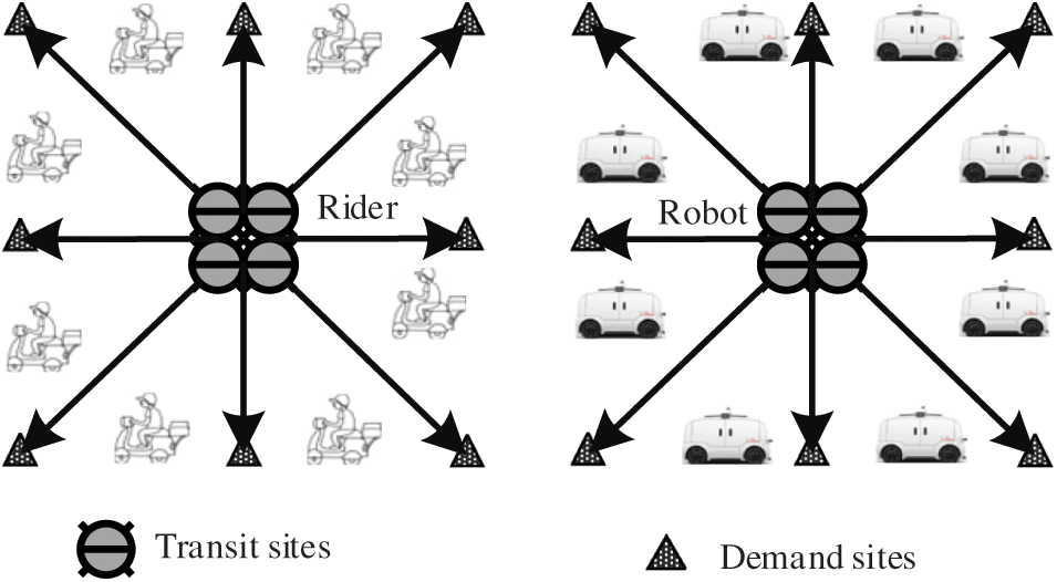
Figure 1: The terminal distribution network
3.1 Costs of Rider Delivery Mode
(1) Fixed costs.
including rider wages, vehicle acquisition and vehicle maintenance costs, among them,
(2) The cost of transportation.
among them,
(3) The cost of fresh-keeping effort.
Among them, the insurance efforts for fresh products are divided into two parts, namely, the fresh-keeping effort cost of fixed distribution centers and movable distribution tools. The preservation cost
(4) The cost of time penalty.
among them,
(5) The cost of performance reward.
where,
3.2 Modeling of Rider Delivery Mode
The first item of the objective function (6) is fixed cost, including total rider salary, vehicle acquisition cost and fixed maintenance cost. The second item is the cost of transportation delivery. The third term is the time penalty cost, and last is performance reward.
subject to,
Specific constraints. Constraint (7) is distance constraint, and
3.3 Costs of Robot Delivery Mode
(1) Fixed costs.
including the purchase cost of the delivery robot and the fixed maintenance cost of the delivery robot, among them,
(2) The cost of transportation.
among them,
(3) The cost of time penalty.
where,
(4) The cost of fresh-keeping effort.
Similar to the rider distribution mode, the machine distribution mode also requires special refrigeration equipment to ensure the freshness of fresh products.
3.4 Modeling of Robot Delivery Mode
The objective function (20) of the robot delivery mode is to minimize the cost. The first term is the fixed cost of the delivery robot. The second item is the transportation cost related to the driving distance. The third term is the time penalty cost.
subject to,
Specific constraints. Constraint (21) is the distance constraint,
There are many uncertain factors in the real market environment, such as the heterogeneity of customer demand at the demand side, the instability of supply and inventory, and even the uncertainty of traffic control on delivery time. With the help of modern technology (big data, machine learning, optimization, etc.), the availability of information is enhanced [27,28]. Affected by these uncertainties, the order quantity also has great uncertainty. The development of modern Internet technology can provide more convenience for the development of the market [29]. In other words, uncertainty factors will directly affect the order demand, and then affect the design of route planning. Considering the interference of potential uncertain factors, we extend the above model through uncertain robust theory [30–33]. The deterministic demand scenario is extended to the uncertain scenario. Its purpose is to achieve the optimal design scheme of path planning on the basis of meeting customer needs to the greatest extent. According to real scenarios, the goal of the stochastic programming model is to minimize the total cost. Based on robust programming theory, we extend the basic model. Define the random variable
Proposition 1. Considering the random demand parameters, the model of rider delivery mode under the deterministic scenario can be extended to the uncertain scenario in Section 3.2, which is named robust counterpart form of rider delivery mode. The interval value uncertainty sets
Robust counterpart form of rider delivery mode:
subject to constraints (7), (8), (9), (10), (11), and, constraints (13), (14).
Considering the uncertain demand parameters, we can get linear inequality (26) with the data varying in the uncertainty set.
Proof of proposition 1. In the rider delivery mode, considering the influence of uncertain demand parameters
Proposition 2. Similar to Proposition 1, considering the interval value uncertain parameter set
Robust counterpart form of robot delivery mode
subject to constraints (21), (22), (23), (24), (25), and, uncertain inequality constraints as (31).
Proof of proposition 2. In the robot delivery mode, considering the influence of uncertain demand parameters, the item
The following difficulties are often faced when solving stochastic optimization models in uncertain demand scenarios. In practical applications, since the probability distribution of random parameters is unknown, it is difficult to solve, even if it is assumed to obey a known probability distribution. First of all, if is a continuous random variable, it involves the calculation of multiple integrals, and the calculation is extremely difficult. Second, the distribution problem we study contains multiple constraints, and there may be no solutions. Finally, there are multiple chance constraints in the path optimization problem. Since the probability distribution of demand is unknown, this constraint may be non-convex, and how to model and calculate is also very difficult to deal with.
Section 5.1 describes the basic data, and Section 5.2 describes the solution steps of the model.
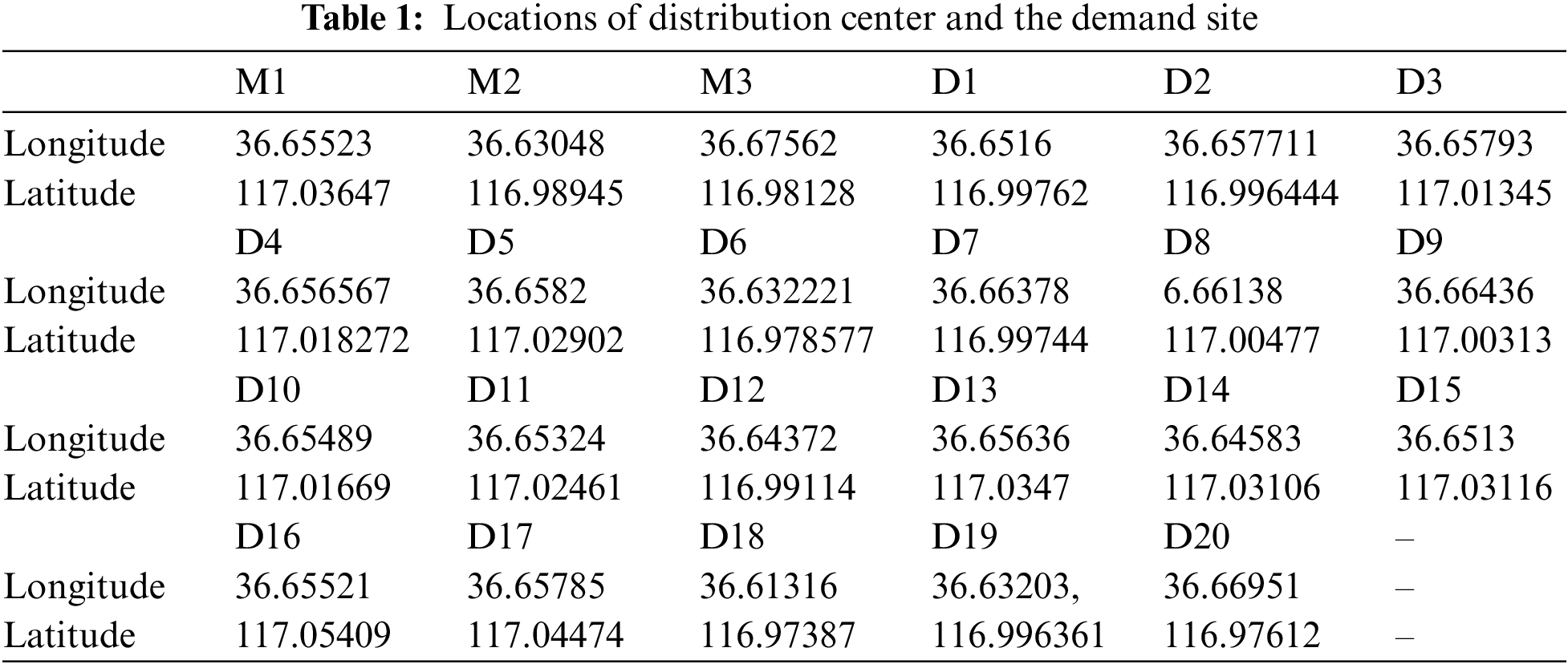
This section takes the data of local transportation companies in Jinan of Shandong as the research object to verify the effectiveness of the proposed distribution model. The information involved in our research mainly comes from Baidu Map, and the transportation cost parameters come from the public data of the network. The distribution center is a supermarket, which distributes fresh agricultural products to nearby demand nodes that may appear randomly. The distribution start point is the supermarket distribution station, and the distribution end point is the community demand site. The distribution service is realized by two modes of transportation, namely the rider distribution mode and the robot mode. According to real-world scenarios, we collect actual data to verify the model. Since there is no standard template case for the distribution of fresh agricultural products, the design scenario of this paper is as follows. There are three distribution centers, namely RT-Mart (Lixia Store), RT-Mart (Shizhong Store), and RT-Mart (Tianqiao Store). There are a total of 20 demand sites, namely, Sanjian Ruifu Garden, Renai Street Community, Qingnian West Road Community, Nanqumen Lane Community, Foshanyuan Community, Rongxiuyuan, Taikangli Community, Linxiang Building, Huajingyuan, Wenhuaxi Road Community, Wenhui Garden, Desheng Homestead, Shun Ai Garden, Crown Villa, Lishan Famous County, Evergrande Emperor Jing, Hongtai Community, Longchang Garden, Langmao Mountain Community, Tianbao New Residence. The order data of the merchant is simulated and generated. The order quantities of each demand site are 260, 320, 410, 450, 380, 280, 300, 460, 450, 310, 220, 340, 410, 350, 340, 280, 390, 460, 350, 360. Taking into account the screening and packaging processes that exist in reality, we set the delivery time for fresh produce delivery to 30–45 min. Taking into account the screening and packaging processes that exist in reality, we set the delivery time for fresh produce delivery to 30–45 min. If it is not delivered within 45 min, a penalty cost will be incurred, and the longer the delay time, the greater the penalty cost. Referring to the real scene, set the relevant parameters of the delivery tool, which are the rider delivery mode and the robot delivery mode. The fixed costs are 4000 and 4500, respectively; The unit delivery cost is 5 and 3, respectively; The average delivery speed is 15 and 12, respectively; The time penalty costs are 10 and 8, respectively; The rated load is 10 and 15, respectively; The unit energy consumption is 2 and 4, respectively; The carbon emission conversion factors are both 0.6101 and 0.6101; The maximum driving distance is set to5 km. The locations (latitude and longitude) of the distribution center and the demand site are shown in Table 1.
We set up the solution framework shown below, and build algorithms to solve the models in Sections 3 and 4. Based on the above basic data, the algorithm framework is designed with Matlab (R 2020) as the programming platform, and the solver Gurobi (9-5) is called to solve the model. The operating system is Windows 10, Core (TM) i5-8300H CPU, computer memory is 8 GB, 512 G SSD, and the frequency is 2.3–3.6 GHz. The specific steps are shown in Fig. 2.
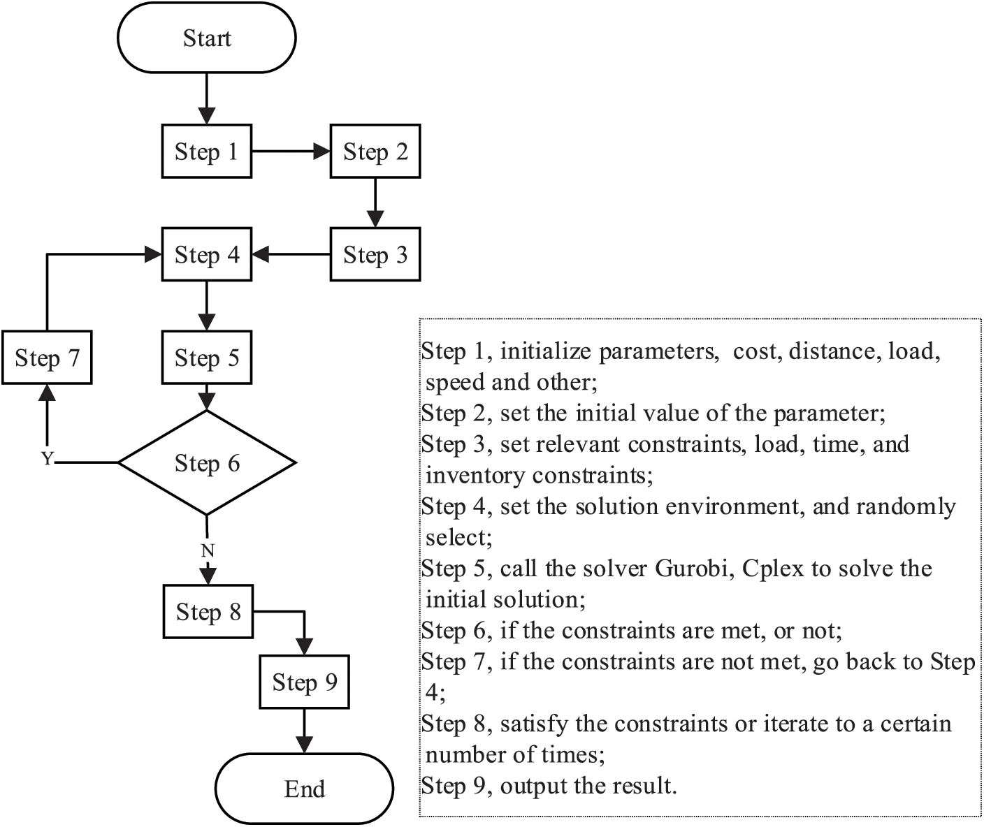
Figure 2: Algorithm process framework
In order to verify the effectiveness of the model, we conduct a comparative analysis of the two delivery modes from multiple dimensions. Section 6.1 compares and analyzes the time efficiency. Section 6.2 describes the influencing factors of cost. Section 6.3 is the robust price of robust counterpart form. Section 6.4 formulates the delivery route planning scheme. Section 6.5 compares the influencing of distribution efficiency.
This section compares the operating efficiency of each model by observing the model operation time. To ensure the validity of the results, all models are run in the same computer environment. This section analyzes the operating efficiency of the four models, and the results are shown. Fig. 3 shows the computational efficiency of the rider delivery and robot delivery mode. In order to facilitate comparison, run in the same computer environment, set the number of sites as the only variable, and observe the model running time. In addition, we also compare and analyze the operation time based on different solvers (Gurobi, Gu and Cplex, Cp). It can be seen from the figure that the rider delivery mode has the highest operating efficiency, and the overall running time is lower than the robot delivery mode. From the details, with the increase of the number of service nodes, the operation time of the model shows an obvious increasing trend. Comparing the three MIRP models, when the number of stations is less than 10, the solution time of Gurobi-based and Cplex-based are not significantly different. When the number of stations is higher than 10, the solution efficiency is obviously reduced and the solution time is prolonged. Among them, the solution efficiency based on Gurobi is about 1.5 times of the solution efficiency based on Cplex. Due to the small site scale of the distribution route optimization problem in this study, a feasible solution can be obtained within 10 s. With the expansion of the model scale, the feasibility of the solution framework based on this framework will decrease, so it is necessary to further optimize the algorithm or change the model framework, design the model and solve it according to the actual demands.
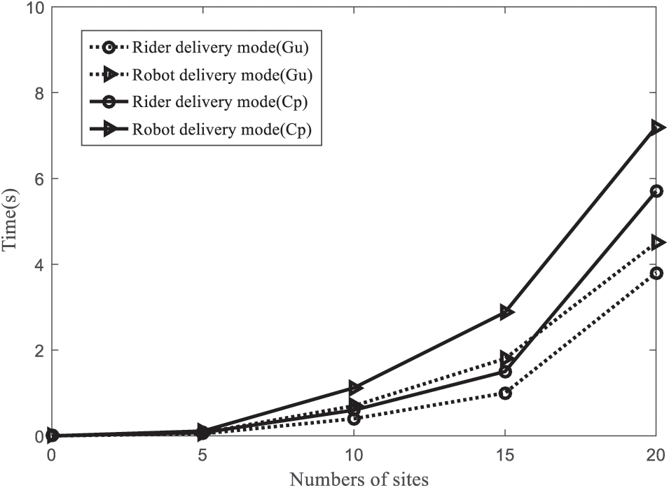
Figure 3: Computational time efficiency
Fig. 4 depicts delivery costs in a 2-week delivery mode. It can be seen that the delivery cost of the rider mode is higher than the cost of the robot delivery mode. In the single-cycle scenario, this difference is not large, but as the delivery cycle increases, the distribution cost shows a clear difference. In a single cycle, compared with the rider delivery mode, the robot delivery mode can save 2,893 CNY. In the daily distribution cycle, compared with the rider delivery mode, the robot delivery mode can save 5,786 CNY. In the weekly delivery cycle, compared with the rider delivery mode, the robot delivery mode can save 40,502 CNY. On the whole, the robot distribution model can save 12.72% of the cost. In the process of practical application, in addition to operating costs, the acquisition cost of distribution tools is also a key factor worthy of attention. Since the research and development of unmanned delivery robot-related technologies is still in its infancy, its configuration costs are high and it relies on professional technicians for maintenance. In the future, if delivery robots can be mass-produced, their efficiency advantages will gradually become apparent as their configuration costs decrease.
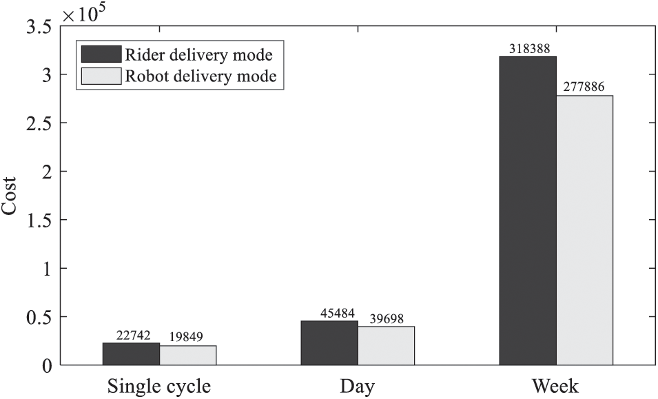
Figure 4: Delivery costs
Fig. 5 analyzes the impact of fluctuations in uncertain demand parameters on total cost. To ensure the unbiasedness of the experiment, all tests were fixed to a normal distribution, and the effect of volatility changes on cost was studied by changing the mean and variance. Through the comparison of numerical cases, it can be found that as the volatility of uncertain parameters increases, the total cost of both the rider delivery mode and the robot delivery mode shows an upward trend. Different modes have different cost rise rates, and the rider delivery mode has a larger cost growth rate, that is, a larger slope. Relative to the rider delivery model. The robot delivery model is not only lower in total cost, but also at a lower rate of cost growth. Therefore, compared with the rider delivery mode, the robot delivery mode has more advantages in terms of economic cost.
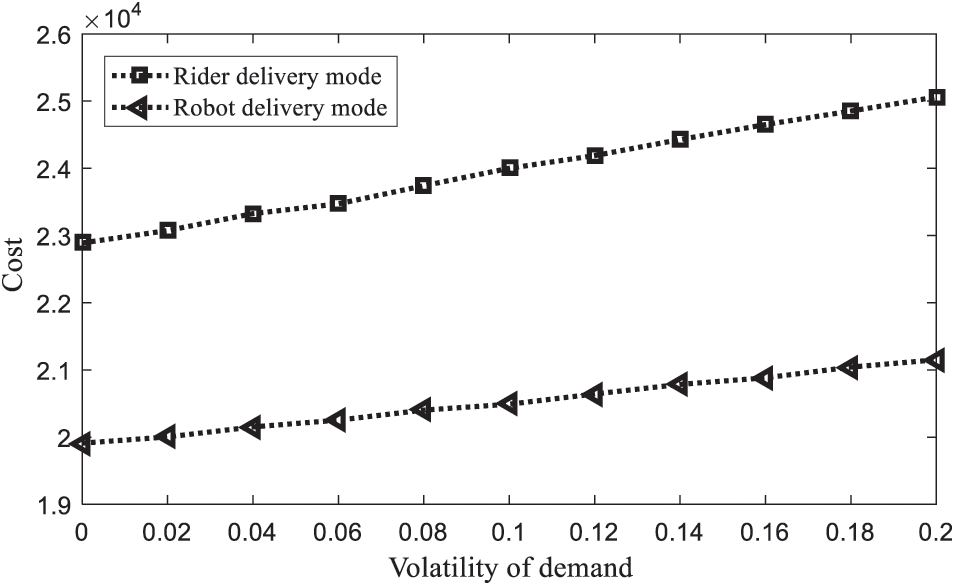
Figure 5: The impact of volatility parameters on costs
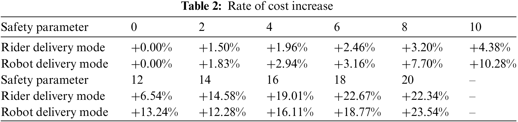
Since the uncertainty of real parameters will disturb the order demand and the number of demand nodes, we introduce robust equivalence theory to resist the uncertainty disturbance. Since the robust equivalent model is a decision under the worst-case scenario, the model has strong robustness. At the same time, these robust equivalent models are bound to pay a certain robust price. To ensure the scientific of comparative experiments, we define the maximum boundary of uncertain demand parameter fluctuation as
We conduct simulations based on actual cases, and the initial delivery path planning scheme is shown in Fig. 6. It can be seen intuitively from the initial path planning scheme that the path planning has the following defects. First, there is the problem of ultra-long-distance transportation, which is bound to increase the cost of delivery, whether it is an unmanned delivery mode or a rider delivery mode. Second, there is the problem of roundabout transportation, which will lead to uneven distribution of distribution resources and waste of distribution resources. Third, there is the problem that individual distribution centers are overburdened, which can easily lead to a backlog of agricultural products in distribution centers, and agricultural products are highly perishable products. Improper management will inevitably lead to greater losses. In order to balance resource allocation, we improved the original model. Respond to real-world needs by optimizing the proportion of riders or robots. The improved path planning scheme is shown in Fig. 7. It can be clearly seen that the path of the overall improved scheme is clearer and more convenient than previous strategies. The problems of circuitous transportation, long-distance transportation and overloading of individual sites are avoided. From the overall optimized distribution route planning scheme, this kind of research can provide intuitive reference suggestions for relevant managers, and has important practical application value.
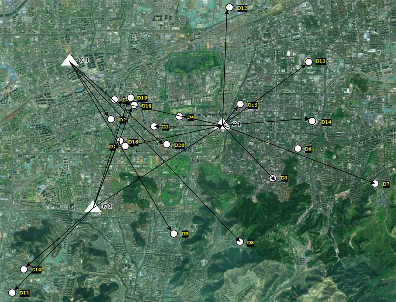
Figure 6: Initial schematic diagram of route planning
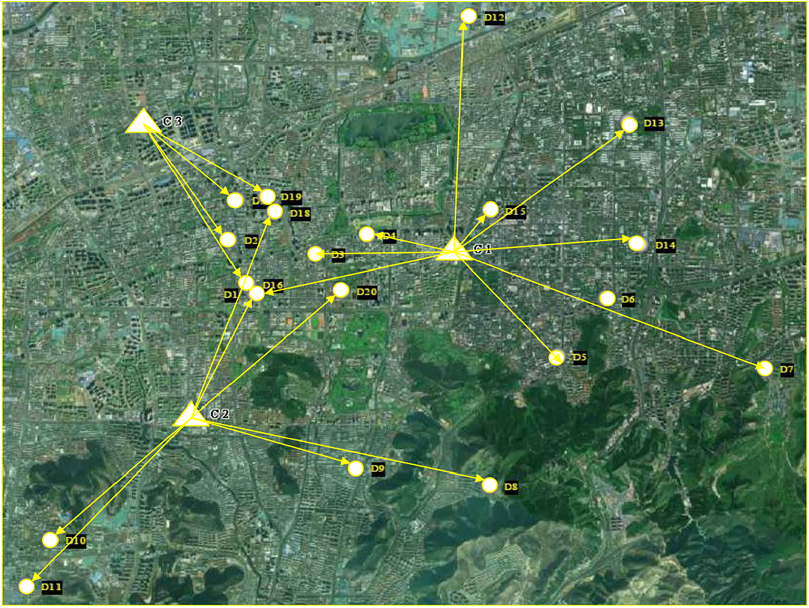
Figure 7: Schematic diagram of route planning after improvement
The logistics service level is described by taking time as a reference, and the on-time rate is described by the difference from the reference time. The performance of the two modes is compared, and management enlightenment is given according to the differences of the modes. The calculation formula of logistics efficiency is,
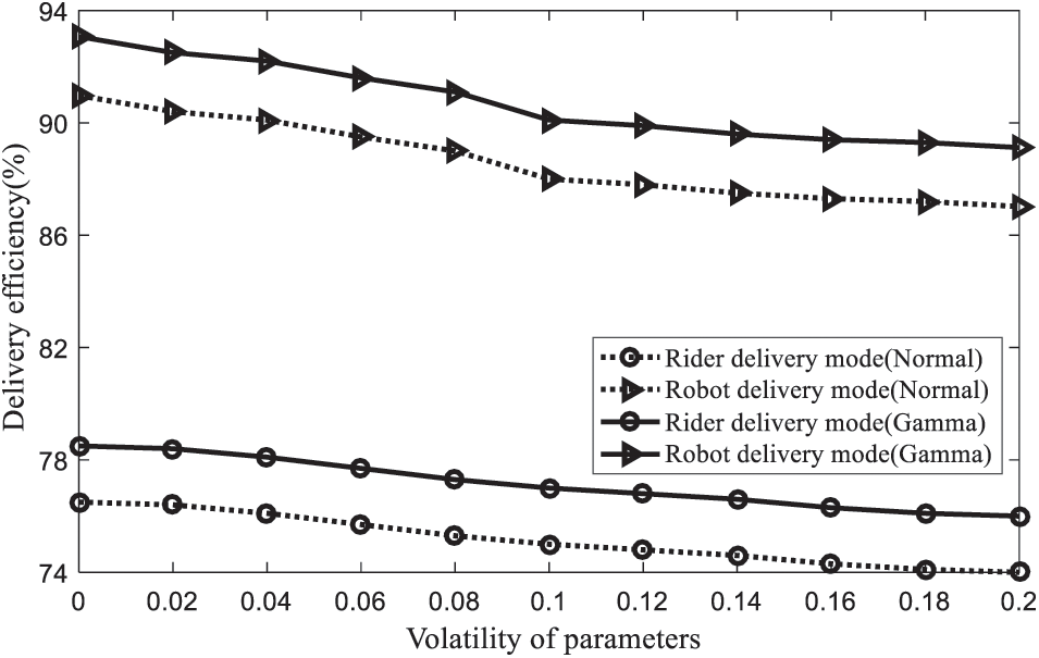
Figure 8: Delivery efficiency
Two common probability distribution functions (normal and gamma distribution) are used as examples to analyze the impact of parameter volatility on distribution efficiency. On the whole, as the uncertainty of demand parameters increases, whether it is a normal distribution or a gamma distribution function, the distribution efficiency shows a downward trend. In other words, the fluctuation of uncertain parameters will inevitably lead to the decline of logistics distribution efficiency, which is an inevitable fact. From the comparison of distribution modes, it can be seen that the overall distribution efficiency of the robot distribution mode is relatively high, which is within the range of 85~95, which is much higher than that of the rider distribution mode, which is in the range of 74~82. In real practice, due to the strong adaptability of robot distribution to weather and road conditions, it also shows a high punctuality rate and service level. In the comparison of distribution functions, it can be seen that the distribution efficiency shows significant differences under different separation functions. This further confirms the importance of forecasting parameters. If uncertain parameters can be accurately evaluated, the improvement of logistics distribution efficiency will be more scientific and feasible. For managers, it is very important for scientific planning and management to analyze the existing parameters in a data-driven way to obtain valuable key parameters.
The terminal distribution network of fresh agricultural products has the problems of low efficiency, high cost and great influence of uncertain factors. Taking the terminal distribution network as the object of modeling, the classic rider distribution mode and the emerging robot distribution mode are analyzed. Considering factors such as fixed cost, transportation cost, time penalty cost, preservation effort cost and performance reward cost in the terminal distribution process, a mixed integer linear integer programming model was constructed. Considering that there is still a lot of uncertainty in the real market environment, in order to resist the interference of uncertainty, we further extend the model to a robust correspondence model. We collected real data from Jinan City, Shandong Province to form a simulation case, verified the proposed strategy, and obtained the optimal distribution routing and inventory schemes for the two distribution modes, and put forward suggestions or improvement schemes for enterprise decision makers.
The simulation experiment case obtains the following insights. In terms of the comparison of the terminal distribution mode, compared with the traditional rider distribution mode, the robot distribution mode can save 12.72% of the cost. If delivery robots can be popularized in the future, their economic benefits and delivery efficiency will be very high. In terms of algorithm efficiency, all the models we designed can obtain feasible solutions within an acceptable time, and the solution efficiency based on Gurobi is higher than that based on Cplex. In terms of delivery route optimization, the routing scheme of our improved scheme is clearer and more convenient than the random assignment strategy. In terms of resisting uncertainty, as the uncertainty of demand parameters increases, the fluctuation of uncertain parameters will inevitably lead to a decline in distribution efficiency. The overall delivery efficiency of the robot delivery mode is much higher than that of the rider delivery mode. In actual operation, due to the strong adaptability of robot distribution to weather and road conditions, it shows a high punctuality rate and service level.
Based on the case insights and the current development status of fresh agricultural product distribution companies, we make the following suggestions. In the scenario of not changing the distribution mode, the terminal distribution enterprises of fresh products should pay attention to the disturbance of uncertain factors on the distribution network, and the quantitative evaluation of uncertain parameters is crucial to the robustness of the distribution network. For enterprises, enterprises should seek profit margins on the basis of ensuring the stability of their supply. The government should strengthen the subsidy for the research and development of high-tech facilities, especially the research and development of equipment and technologies such as delivery robots. Although our research can prove that the efficiency of the robot delivery model is better than that of the traditional model, the application of technology is very important for general or small delivery. Enterprises are still a problem, mainly due to the limitation of technical threshold. If the government can provide better technical support or subsidies, it will greatly promote the improvement of the terminal distribution network.
There are still some points that need to be improved in the current research. For example: consider the joint distribution of multi-terminal distribution companies, consider the uncertainty of time windows, the path planning of delivery robots in three-dimensional space, consider customer satisfaction, etc. These factors will be considered in future research.
Acknowledgement: The authors are extremely appreciative to the editors and anonymous reviewers for the insightful comments and suggestions.
Funding Statement: The authors received no specific funding for this study.
Author Contributions: The authors confirm contribution to the paper as follows: study conception and design: Z. Wu, Y. Feng; data collection: X.Y. Teng; analysis and interpretation of results: F. Yang, Z. Wu, X.Y. Teng; draft manuscript preparation: F. Yang. All authors reviewed the results and approved the final version of the manuscript.
Availability of Data and Materials: All of data used in this paper can be found in the published paper.
Conflicts of Interest: The authors declare that they have no conflicts of interest to report regarding the present study.
References
1. He, B., Gan, X., Yuan, K. (2019). Entry of online presale of fresh produce: A competitive analysis. European Journal of Operational Research, 272(1), 339–351. [Google Scholar]
2. Yan, B., Han, L. G. (2022). Decisions and coordination of retailer-led fresh produce supply chain under two-period dynamic pricing and portfolio contracts. Rairo-Operations Research, 56(1), 349–365. [Google Scholar]
3. Villarreal, B., Garza-Reyes, J. A., Kumar, V. (2016). Lean road transportation—A systematic method for the improvement of road transport operations. Production Planning & Control, 27(11), 865–877. [Google Scholar]
4. Li, Y. K., Niu, W. J., Tian, Y. Z., Chen, T., Xie, Z. Q. et al. (2022). Multiagent reinforcement learning-based signal planning for resisting congestion attack in green transportation. IEEE Transactions on Green Communications and Networking, 6(3), 1448–1458. [Google Scholar]
5. Zhao, X., Lin, W., Cen, S., Zhu, H., Duan, M. et al. (2021). The online-to-offline (O2O) food delivery industry and its recent development in China. European Journal of Clinical Nutrition, 75(2), 232–237. [Google Scholar] [PubMed]
6. Niu, B., Li, Q., Mu, Z., Chen, L., Ji, P. (2021). Platform logistics or self-logistics? Restaurants’ cooperation with online food-delivery platform considering profitability and sustainability. International Journal of Production Economics, 234, 108064. [Google Scholar]
7. Wang, Y., Zhang, D., Liu, Q., Shen, F., Lee, L. H. (2016). Towards enhancing the last-mile delivery: An effective crowd-tasking model with scalable solutions. Transportation Research Part E: Logistics and Transportation Review, 93(6), 279–293. [Google Scholar]
8. Qi, W., Li, L., Liu, S., Shen, Z. J. M. (2018). Shared mobility for last-mile delivery: Design, operational prescriptions, and environmental impact. Manufacturing & Service Operations Management, 20(4), 737–751. [Google Scholar]
9. Chen, X., Wang, X., Jiang, X. (2016). The impact of power structure on the retail service supply chain with an O2O mixed channel. Journal of the Operational Research Society, 67(2), 294–301. [Google Scholar]
10. Harfina, D. M., Zaini, Z., Wulung, W. J. (2021). Disinfectant spraying system with quadcopter type unmanned aerial vehicle (UAV) technology as an effort to break the chain of the COVID-19 virus. Journal of Robotics and Control, 2(6), 502–507. [Google Scholar]
11. Eichleay, M., Evens, E., Stankevitz, K., Parker, C. (2019). Using the unmanned aerial vehicle delivery decision tool to consider transporting medical supplies via drone. Global Health: Science and Practice, 7(4), 500–506. [Google Scholar] [PubMed]
12. Goodchild, A., Toy, J. (2018). Delivery by drone: An evaluation of unmanned aerial vehicle technology in reducing CO2 emissions in the delivery service industry. Transportation Research Part D: Transport and Environment, 61, 58–67. [Google Scholar]
13. Sung, I., Nielsen, P. (2020). Zoning a service area of unmanned aerial vehicles for package delivery services. Journal of Intelligent & Robotic Systems, 97(3), 719–731. [Google Scholar]
14. Schenone, S., Azhar, M., Ramírez, C. A. V., Strozzi, A. G., Delmas, P. et al. (2022). Mapping the delivery of ecological functions combining field collected data and unmanned aerial vehicles (UAVs). Ecosystems, 25(4), 948–959. [Google Scholar]
15. Nicosevici, T., Garcia, R. (2012). Automatic visual bag-of-words for online robot navigation and mapping. IEEE Transactions on Robotics, 28(4), 886–898. [Google Scholar]
16. Kapser, S., Abdelrahman, M. (2020). Acceptance of autonomous delivery vehicles for last-mile delivery in Germany-Extending UTAUT2 with risk perceptions. Transportation Research Part C: Emerging Technologies, 111(2), 210–225. [Google Scholar]
17. Yu, S., Puchinger, J., Sun, S. (2022). Van-based robot hybrid pickup and delivery routing problem. European Journal of Operational Research, 298(3), 894–914. [Google Scholar]
18. Boysen, N., Schwerdfeger, S., Weidinger, F. (2018). Scheduling last-mile deliveries with truck-based autonomous robots. European Journal of Operational Research, 271(3), 1085–1099. [Google Scholar]
19. Kitjacharoenchai, P., Min, B. C., Lee, S. (2020). Two echelon vehicle routing problem with drones in last mile delivery. International Journal of Production Economics, 225, 107598. [Google Scholar]
20. Chen, C., Demir, E., Huang, Y., Qiu, R. (2021). The adoption of self-driving delivery robots in last mile logistics. Transportation Research Part E: Logistics and Transportation Review, 146, 102214. [Google Scholar] [PubMed]
21. Bergmann, F. M., Wagner, S. M., Winkenbach, M. (2020). Integrating first-mile pickup and last-mile delivery on shared vehicle routes for efficient urban e-commerce distribution. Transportation Research Part B: Methodological, 131, 26–62. [Google Scholar]
22. Liu, D., Yan, P., Pu, Z., Wang, Y., Kaisar, E. I. (2021). Hybrid artificial immune algorithm for optimizing a Van-Robot E-grocery delivery system. Transportation Research Part E: Logistics and Transportation Review, 154(4), 102466. [Google Scholar]
23. Bakach, I., Campbell, A. M., Ehmke, J. F. (2021). A two-tier urban delivery network with robot-based deliveries. Networks, 78(4), 461–483. [Google Scholar]
24. Heimfarth, A., Ostermeier, M., Hübner, A. (2022). A mixed truck and robot delivery approach for the daily supply of customers. European Journal of Operational Research, 303, 401–421. [Google Scholar]
25. Simoni, M. D., Kutanoglu, E., Claudel, C. G. (2020). Optimization and analysis of a robot-assisted last mile delivery system. Transportation Research Part E: Logistics and Transportation Review, 142, 102049. [Google Scholar]
26. Qin, H., Wei, Y., Zhang, Q., Ma, L. (2021). An observational study on the risk behaviors of electric bicycle riders performing meal delivery at urban intersections in China. Transportation Research Part F: Traffic Psychology and Behaviour, 79, 107–117. [Google Scholar]
27. Qu, S. J., Xu, L., Mangla, S. K., Chan, F. T. S., Zhu, J. L. et al. (2022). Matchmaking in reward-based crowdfunding platforms: A hybrid machine learning approach. International Journal of Production Research. https://doi.org/10.1080/00207543.2022.2121870 [Google Scholar] [CrossRef]
28. Qu, S., Shu, L., Yao, J. (2022). Optimal pricing and service level in supply chain considering misreport behavior and fairness concern. Computers & Industrial Engineering, 174, 108759. [Google Scholar]
29. Zhou, Y., Zhang, Y., Goh, M. (2023). Platform responses to entry in a local market with mobile providers. European Journal of Operational Research, 309(1), 236–251. https://doi.org/10.1016/j.ejor.2023.01.020 [Google Scholar] [CrossRef]
30. Qu, S., Li, Y., Ji, Y. (2021). The mixed integer robust maximum expert consensus models for large-scale GDM under uncertainty circumstances. Applied Soft Computing, 107, 107369. [Google Scholar]
31. Bai, Q. G., Xu, J. T., Zhang, Y. Z. (2022). The distributionally robust optimization model for a remanufacturing system under cap-and-trade policy: A newsvendor approach. Annals of Operations Research, 309(2), 731–760. [Google Scholar]
32. Ji, Y., Li, H. H., Zhang, H. J. (2022). Risk-averse two-stage stochastic minimum cost consensus models with asymmetric adjustment cost. Group Decision and Negotiation, 31(2), 261–291. [Google Scholar] [PubMed]
33. Wei, J., Qu, S., Wang, Q., Luan, D., Zhao, X. (2022). The novel data-driven robust maximum expert mixed integer consensus modelsunder multi-role’s opinions uncertainty by considering non-cooperators. IEEE Transactions on Computational Social Systems, 3192897. [Google Scholar]
Cite This Article
 Copyright © 2024 The Author(s). Published by Tech Science Press.
This work is licensed under a Creative Commons Attribution 4.0 International License , which permits unrestricted use, distribution, and reproduction in any medium, provided the original work is properly cited.
 Downloads
 Citation Tools