
 Submit a Paper
 Propose a Special lssue
 Open Access
ARTICLE
Research and Application of a Multi-Field Co-Simulation Data Extraction Method Based on Adaptive Infinitesimal Element
1 School of Mechanical Engineering, Sichuan University, Chengdu, 610065, China
2 Innovation Method and Creative Design Key Laboratory of Sichuan Province, Sichuan University, Chengdu, 610065, China
* Corresponding Author: Wenqiang Li. Email:
Computer Modeling in Engineering & Sciences 2024, 138(1), 321-348. https://doi.org/10.32604/cmes.2023.029053
Received 29 January 2023; Accepted 05 May 2023; Issue published 22 September 2023
 View Full Text
 Download PDF
Abstract
Regarding the spatial profile extraction method of a multi-field co-simulation dataset, different extraction directions, locations, and numbers of profiles will greatly affect the representativeness and integrity of data. In this study, a multi-field co-simulation data extraction method based on adaptive infinitesimal elements is proposed. The multi-field co-simulation dataset based on related infinitesimal elements is constructed, and the candidate directions of data profile extraction undergo dimension reduction by principal component analysis to determine the direction of data extraction. Based on the fireworks algorithm, the data profile with optimal representativeness is searched adaptively in different data extraction intervals to realize the adaptive calculation of data extraction micro-step length. The multi-field co-simulation data extraction process based on adaptive microelement is established and applied to the data extraction process of the multi-field co-simulation dataset of the sintering furnace. Compared with traditional data extraction methods for multi-field co-simulation, the approximate model constructed by the data extracted from the proposed method has higher construction efficiency. Meanwhile, the relative maximum absolute error, root mean square error, and coefficient of determination of the approximation model are better than those of the approximation model constructed by the data extracted from traditional methods, indicating higher accuracy, it is verified that the proposed method demonstrates sound adaptability and extraction efficiency.Graphic Abstract
Keywords
Nomenclature
| PCA | Principal component analysis |
| FWA | Fireworks algorithm |
| RMAE | Relative maximum absolute error |
| RMAE | Root mean square error |
| R2 | Coefficient of determination |
With the continuous expansion of modern engineering system scales, excessive costs of physical experiments for complex engineering systems have become a significant limitation to developing innovative engineering designs [1–3]. Through multi-field co-simulation based on the multi-field model, the coupling relations between parameters of each field can be fully taken into account and the simulation results of complex multi-field problems can be obtained [4]. Predicting the structural life and reliability of complex engineering systems is gaining importance in the design process [5–7], yet complex engineering systems are usually under multiple physical field couplings. Hence, multi-field co-simulation has become the main numerical simulation method utilized by researchers to solve complex engineering system problems in recent years [8,9]. As the multi-field co-simulation dataset accommodates multiple physical field datasets in the same space and each field's data is coupled and changeable, the multi-field co-simulation dataset demonstrates features of a large data amount and anisotropy in data distribution. Inappropriate data extraction methods will lead to low data extraction efficiency and affect the representativeness and complete distribution of data samples. Therefore, extracting field data samples with high representativeness and integrity from multi-field dataset with efficiency becomes the key technology to achieve multi-field co-simulation data post-processing. Zhou et al. used the multi-field co-simulation method with flow-thermal coupling to determine the flow field velocity and temperature field distribution of multiple profiles of the Nine-Spacer Nozzle structure [10]. In [11], the motion process of the control rod driving mechanism in nuclear fuel assembly has been simulated utilizing the multi-field co-simulation method with the coupling of the motion field, electromagnetic field and flow field. The motion characteristics of the control rod driving mechanism and variation data of the flow field and electromagnetic field in the central profile have also been obtained from the simulation results. The multi-field co-simulation data extraction process of the control rod drive mechanism is also discussed in [12,13]. The effect of pulse operation on the thermal stress response of virtual test blanket module has been examined by Ying et al. [14] using transient thermal-fluid-stress multi-field coupling analysis, and the simulation data of temperature field and thermal stress field on the outer surface and central profile of the structure have been obtained. A new flow field-thermal field-electric field multi-physical field numerical model was proposed in [15] to predict the performance of thermoelectric units for fluid waste heat recovery. The simulation results exhibit the temperature field distribution on the whole outer surface of the generator and transient electromagnetic furnace and the electric field voltage data on the upper surface of the transient electromagnetic furnace. A three-dimensional fluid-thermal-structural multi-physical interaction simulation model for aluminium extrusion process has been established by Maher et al. in [16]. By coupling the simulation model with the structural mechanics analysis, the stress distribution in the die under fluid pressure and thermal load is simulated, and the full three-dimensional results in the processes of temperature distribution, velocity distribution, von Mose stress distribution, equivalent strain distribution and pressure distribution of selected profiles are provided and analyzed. In [17], the three-dimensional fluid-thermal-structural multi-field coupling analysis of the cooling sleeve of supersonic combustion ramjet (scramjet) engine has been performed to extract the data of flow field, temperature field and stress-strain field on the inner surface of the cooling channel, and to predict the structural life of the cooling sleeve. The interlaced fluid-solid coupling algorithm is used by Ko et al. [18] to simulate the internal and external flow field changes of a launch vehicle and demonstrate the flow field and temperature field in the central profile of the launch vehicle. Meanwhile, the unsteady motion of separated rocket booster is predicted using the external flow analysis of the pneumatic-dynamic coupling solver. The internal flow field of the umbrella wind turbine was simulated in [19], with the velocity field and pressure field data in profiles of 0°, 45° and 60° shrinkage angles extracted, providing a theoretical basis for further improving the power regulation mechanism of umbrella wind turbines. Siregar et al. [20] conducted numerical simulation on the temperature field and flow field in inductively coupled thermal plasma (ICTP) extracting and displaying the temperature field in Z profile of plasma torch and discussed the effects of gas composition and power supply on the temperature field of thermal plasma. The operation of high temperature and high pressure furnace equipment was simulated in [21–25] via flow-thermal coupling multi-field co-simulation analysis, and the temperature fields and flow field distributions of multiple profiles of the furnace body have been extracted and displayed. To sum up, the research of multi-field co-simulation data extraction method has made positive progress. According to different application scenarios, a more reasonable spatial profile datasets extraction method is proposed, and partial data of multiple physical fields are obtained, which provides a basis for the optimization design of equipment structure.
At present, the data samples of multi-field co-simulation field are mainly extracted by selecting a single or multiple spatial profile datasets of field. Highly representative and complete simulation data samples will facilitate accurate reflection on the performance of complex engineering equipment, which helps the optimization on the structure of engineering equipment. However, large data amount and data distribution anisotropy of multi-field co-simulation dataset determines that the selection of direction, number and position of the profile will greatly affect the representativeness and integrity of field data sample extraction, and determines the efficiency of data extraction directly. Therefore, a multi-field co-simulation data extraction method based on adaptive infinitesimal elements is hereby proposed in this study. A multi-field co-simulation dataset has been constructed based on related infinitesimal elements, a characteristic direction determination method based on principal component analysis for effective determination of profile direction is introduced, and an adaptive micro-step length determination method based on fireworks algorithm to select appropriate number and position of profiles is expounded. The aforementioned address the two key techniques of data extraction. The method has also been applied to the data extraction process of multi-field co-simulation dataset of sintering furnace, and the results have been compared with traditional data extraction methods to verify the rationality and effectiveness of the proposed method.
2 Multi-Field Co-Simulation Data Extraction Method Based on Infinitesimal Element Method
Multi-field co-simulation dataset, as a continuous dataset composed of complex multi-physical fields distributed along the simulation space, has the characteristics of large data amount and anisotropy in data distribution. In case only a few feature profile datasets are extracted from a multi-field co-simulation dataset, the data samples would be too small to represent the characteristics of multi-field data; yet if too much data is extracted, excessive representation of field data sets will also affect the extraction efficiency. Additionally, unreasonable selection of profile direction will damage the distribution integrity and representativeness of data samples as well. In this study, the correlation between adjacent profile datasets is analyzed by the infinitesimal element method, and the representative profile datasets are extracted to express the distribution characteristics of multi-field dataset. The principal component analysis method is used to determine the direction of profile and the firework algorithm is used to calculate the micro-step length adaptively.
2.1 Construction of Multi-Field Co-Simulation Dataset Based on Related Micro-Element
Due to the coupling effect of multi-physical fields in the simulation process, the multi-field co-simulation dataset comes with the characteristic of multi-field data coupling, as well as complex and changeable data field in the same space. Therefore, the multi-field co-simulation dataset can be established using the same reference frame in the same simulation space. In accordance with the continuity of multi-field data, m profile micro-datasets (data infinitesimal elements) in any simulation direction space can be extracted from each physical field simulation dataset of the multi-field co-simulation dataset composed of S physical field couplings. The relations between each dataset are as follows:
where V is the same simulation space where multiple physical field reside; x, y and z are coordinates in the simulation space;
If two data infinitesimal elements in the same physical field demonstrate low correlation, they will be regarded as unrelated, otherwise they will be considered repeating as related infinitesimal elements. The defined value
where X is the number of sampling points in each micro-dataset;
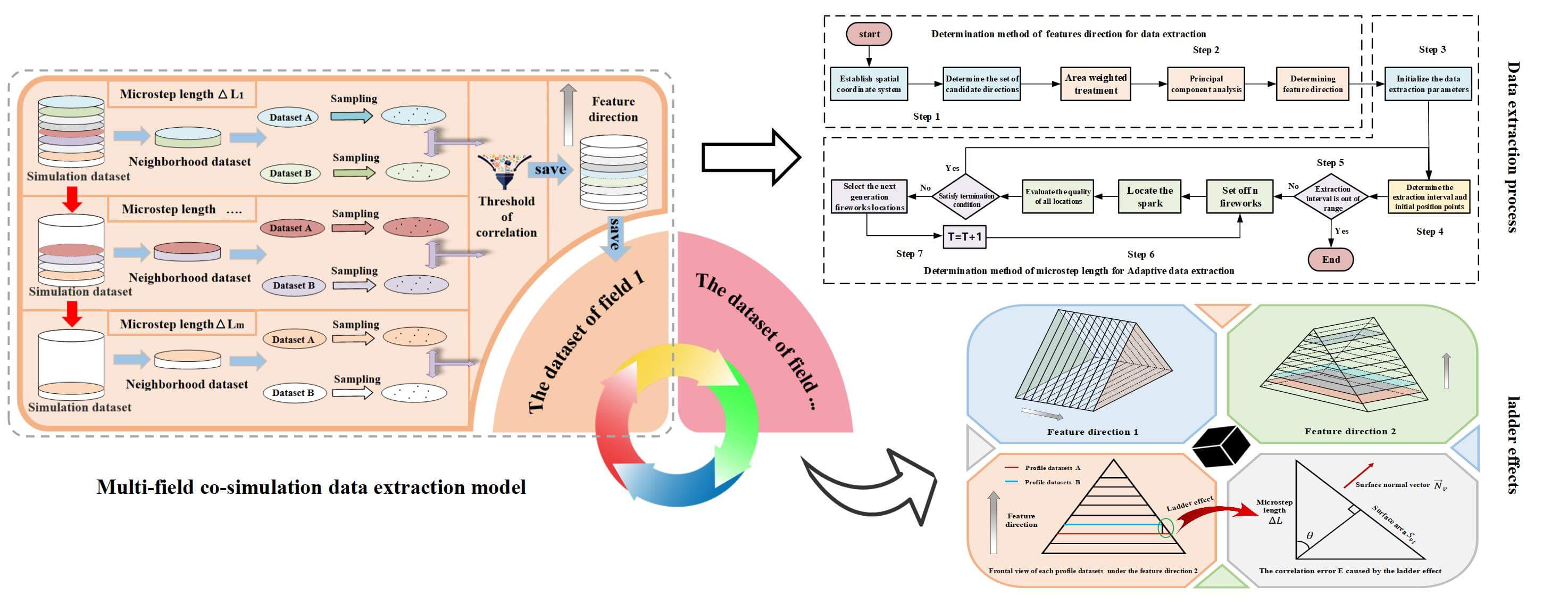
To extract representative and complete samples of multi-field dataset, a multi-field co-simulation data sample extraction model based on the concept of infinitesimal element has been proposed in the current study. Each physical field simulation dataset of a multi-field co-simulation dataset can be sliced into m profile micro-datasets in a certain direction, with the direction of micro-datasets segmentation defined as the characteristic direction
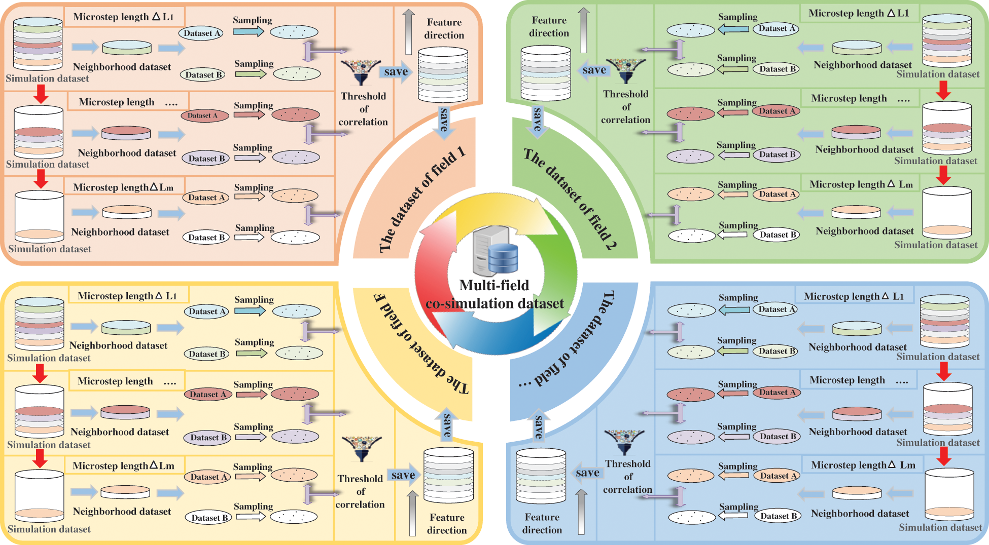
Figure 1: Multi-field co-simulation data extraction model based on related infinitesimal elements
To facilitate the extraction of multi-field co-simulation data samples, two key technical problems are crucial: the selection of data infinitesimal elements’ characteristic direction and the determination of micro-step length of data infinitesimal elements. Firstly, as the spatial characteristics of multi-field co-simulation dataset are different, different data infinitesimal elements will be obtained from slicing along different characteristic directions. Also, different characteristic directions will have a significant impact on the simulation data extraction results. Secondly, extraction data with different micro-step length will lead to different data processing quantities and data extraction accuracy, which will greatly affect the reliability of data extraction results.
2.2 Determination Method of the Characteristic Direction for Data Extraction
When the micro-step length approaches infinitesimal, two profile micro-datasets in the neighborhood dataset can be considered to be fully correlated. However, the micro-step length cannot approach infinitesimal in reality and if there is an angle between the spatial surface of the simulation dataset and the selected characteristic direction, a ladder effect will occur between the two profile micro-datasets in the neighborhood dataset, leading to different data sampling area of the two profile micro-datasets and ultimately the error of correlation calculation. This error is hereby defined as the correlation error E, as shown in Fig. 2. Therefore, it is similar to the determination of printing direction in additive manufacturing [27,28]: when the spatial surface of the simulation dataset has been determined, the selection of characteristic direction should reduce the correlation error E of data extraction as much as possible.
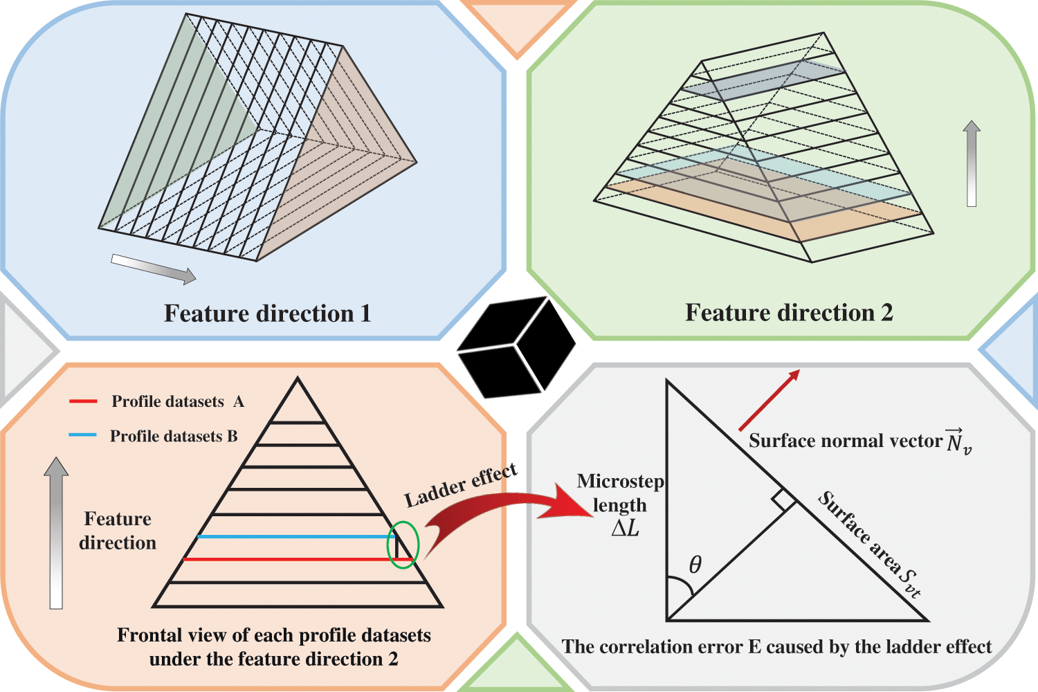
Figure 2: Effects of different characteristic directions and ladder effects on the same spatial simulation dataset
From the analysis, when the selected characteristic direction is parallel or perpendicular to the simulation dataset surface, the correlation error caused by the ladder effect can be minimized. Hence, all the surface unit normal vectors
where
Calculating the correlation errors with the unit normal vector of each surface as the characteristic direction successively will lead to large calculation amount, therefore dimension reduction of the candidate characteristic direction set
In which, the sample space of the new area-weighted normal vector is
First, the average normal vector
The difference between each area-weighted normal vector and the average normal vector is calculated, and the difference value vector
Construct a covariance matrix
In which,
Given that the covariance matrix C is a real symmetric matrix, the Jacobi SVD method can be utilized to decompose the covariance matrix C via singular value decomposition. Three eigenvalues and their corresponding eigenvectors can be obtained, from which the direction with the smallest correlation error can be selected and determined as the final candidate characteristic direction.
2.3 Determination Method of Microstep Length for Adaptive Data Extraction
The selection of micro-step length
The fireworks algorithm, a global optimization algorithm, simulates the phenomenon of fireworks explosion to conduct global search [32]. Fig. 3 is the optimization framework of the fireworks algorithm. In this study, the fireworks algorithm is deployed in segmented intervals in search of the optimal data extraction positions, so as to determine the micro-step length. To begin, the initial profile micro-dataset A is set up and the interval of the next extraction interval to be optimized is calculated. The fitness function
In which, X is the number of sampling points in each micro-dataset;
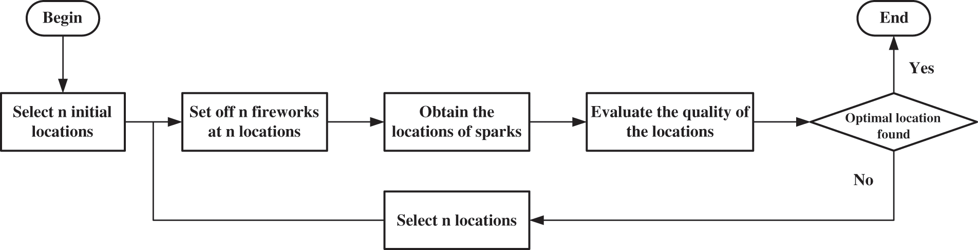
Figure 3: Optimization framework of fireworks algorithm
The optimal termination condition is set as when the number of iterations
Initialize data extraction parameters: the initial profile micro-dataset A is determined; taking the characteristic direction as the coordinate axis and the position of micro-dataset A in the characteristic direction as the origin to establish a single-dimensional coordinate system;
Determine the data interval L to be optimized, and set the initial position point: if i = 1, then L =
Based on the above, to address the selection of different micro-step lengths in different regions of the simulation dataset, an adaptive adjustment coefficient S is introduced in the current study. It is able to adaptively adjust the range of interval to be optimized according to the data characteristics of different areas, improving the search efficiency of FWA optimization, finding out the position of data extraction profile as soon as possible, so as to determine the micro-step length
k (k > 0) is the slope trend factor that can change the adjustment amplitude of S. It is determined according to the spatial range and data extraction accuracy of the simulation dataset. INT is defined as a rounding function to ensure that the length of the optimization interval is an integer.
Decide the termination condition of data sample extraction: in case the extraction interval is beyond the scope of the simulation dataset space, data sample extraction of dataset shall be terminated. Otherwise, it shall be continued.
Fireworks algorithm optimization: n fireworks are placed at n fireworks placement points in the interval to be optimized. The fitness of each firework
In which,
In which,
Based on the mapping rule, the position
Initialize the location of the explosion spark:
Set
Hence,
If
Then
The minimum
Decide the termination condition of optimization: decide whether the number of iterations T meets the optimal termination condition, i.e.,
Screen the next generation fireworks: n next generation firework location points are set based on selection probability
where K is a collection of all fireworks and exploding sparks.
3 Data Extraction Process of Multi-Field Co-Simulation Based on Adaptive Infinitesimal Elements
Based on the aforementioned determination methods for characteristic direction and micro-step length, a multi-field co-simulation data extraction process based on adaptive infinitesimal elements is hereby introduced, as shown in Fig. 4.
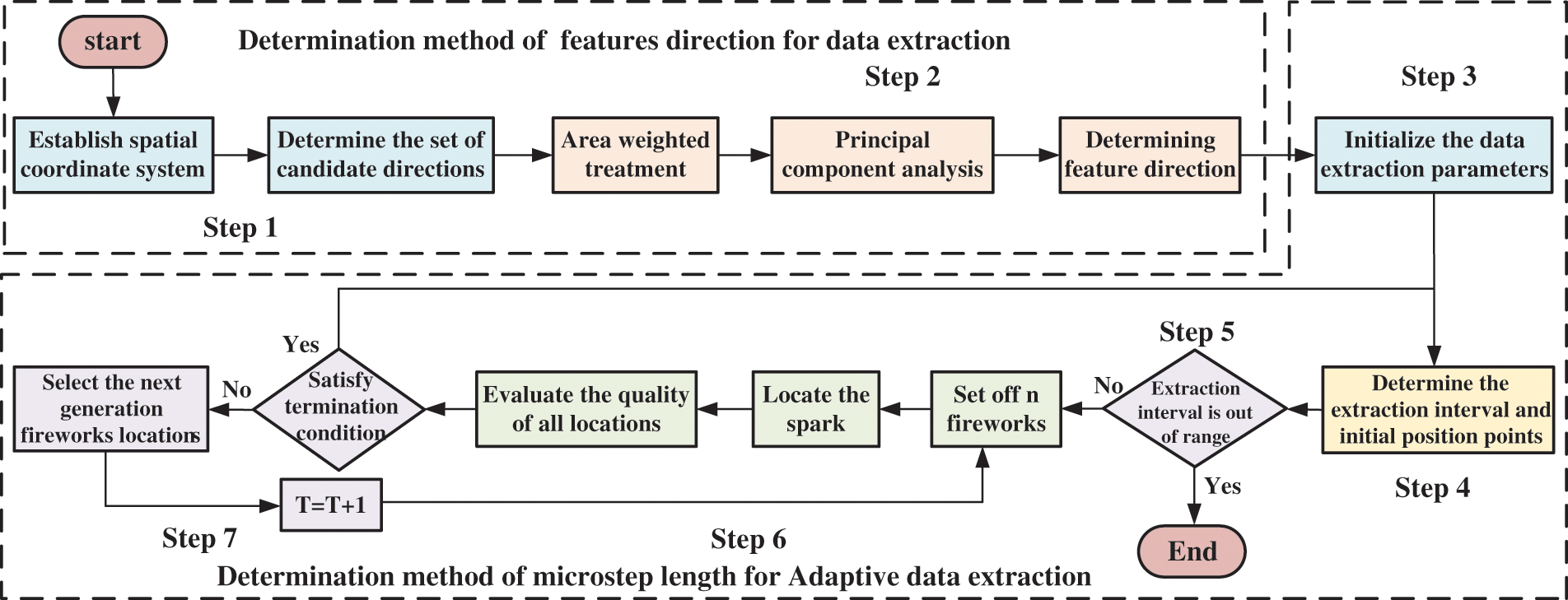
Figure 4: Data extraction process of multi-field co-simulation based on adaptive infinitesimal elements
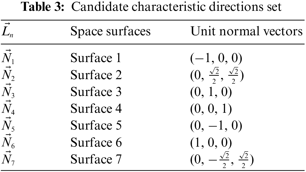
Step 1: create a candidate direction set. Establish the 3D spatial coordinate system of the simulation dataset, and the unit normal vectors
Step 2: determine the characteristic direction. Area weighted normal vector
Step 3: initialize the data extraction parameters. The initial profile micro-dataset A is determined. The single-dimensional coordinate system is established. The initial optimal interval length
Step 4: determine the interval to be optimized. The range of extraction interval to be optimized is determined, and n fireworks position points are initially set in the interval to be optimized with initially setting
Step 5: determine the termination conditions of data sample extraction. Determine whether the extraction interval to be optimized is beyond the scope of the simulation dataset. If so, end the extraction process, otherwise proceed to the next step.
Step 6: fireworks algorithm optimization. The fireworks are placed at the n selected fireworks location points, and the fitness values of the fireworks and spark are calculated. The smallest position point is selected from the fitness function value of all fireworks and explosion spark position points and compared with the value of
Step 7: determine termination condition of optimization. Termination shall be subject to whether the number of iterations T meets the termination condition of optimization
Pressure sintering furnace is a type of industrial equipment for sintering cemented carbides, as shown in Fig. 5. Cemented carbide sintering contains a number of processes, such as hydrogen dewaxing, vacuum sintering, pressure sintering and pressure relief cooling. It is a typical coupling process of the flow field and thermal field with the control of temperature field in the sintering furnace exerting significant influence on the quality of sintered products. Due to factors as measured space and heat transfer conditions, direct multi-point temperature measurement in the furnace is not always feasible. Therefore, it is of great significance to examine the temperature field in the furnace by using simulation technology. In this study, the flow-thermal multi-field co-simulation of pressure sintering furnace in sintering process is carried out, and the simulation data are extracted by the proposed multi-field co-simulation data extraction method in order to obtain the temperature field distribution pattern in the furnace efficiently. The atmosphere field (flow field) distribution pattern can be obtained in the same way. The two fields together constitute the pressure sintering furnace multi-field co-simulation dataset.
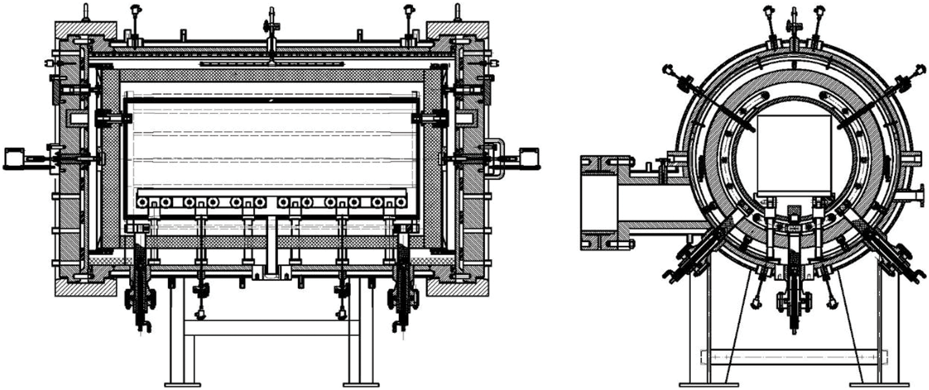
Figure 5: Assembly drawing of a pressure sintering furnace
In this study, a simplified fluid domain model in sintering furnace has been established, as shown in Fig. 6. In the stage of hydrogen dewaxing, the 14 heating rods are sparsely installed above and densely installed below, and the furnace is continuously heated to of process node temperature at a total power of 500 Kw. Hydrogen is induced at the rate of 0.85 m/s into the inlet to fill the space between the thermal insulation layer and the porous graphite layer, and the wax gas produced by dewaxing of the alloy and hydrogen is discharged through the lower outlet.
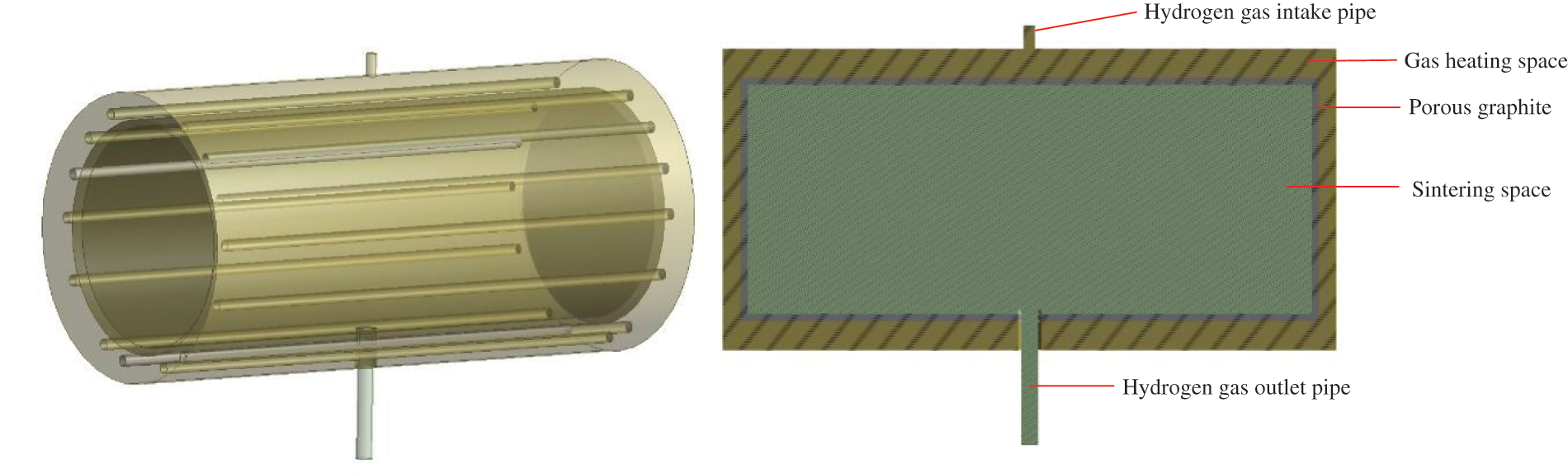
Figure 6: Simplified fluid domain model of pressure sintering furnace
Set parameters and boundary conditions as shown in Tables 1 and 2. Establish fluid simulation model of sintering furnace based on the aforementioned working conditions, and the boundary of the model is shown in Fig. 7.
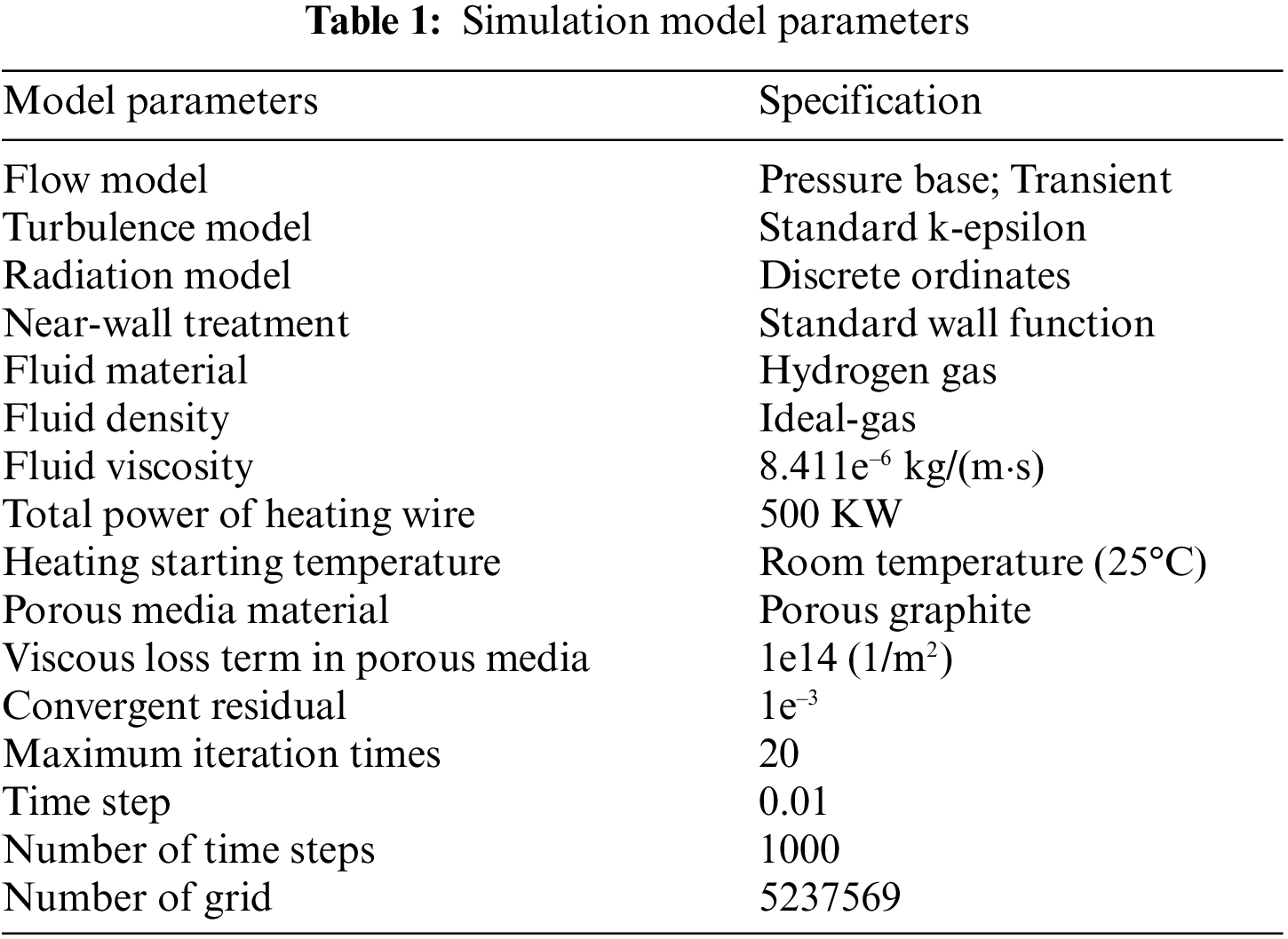
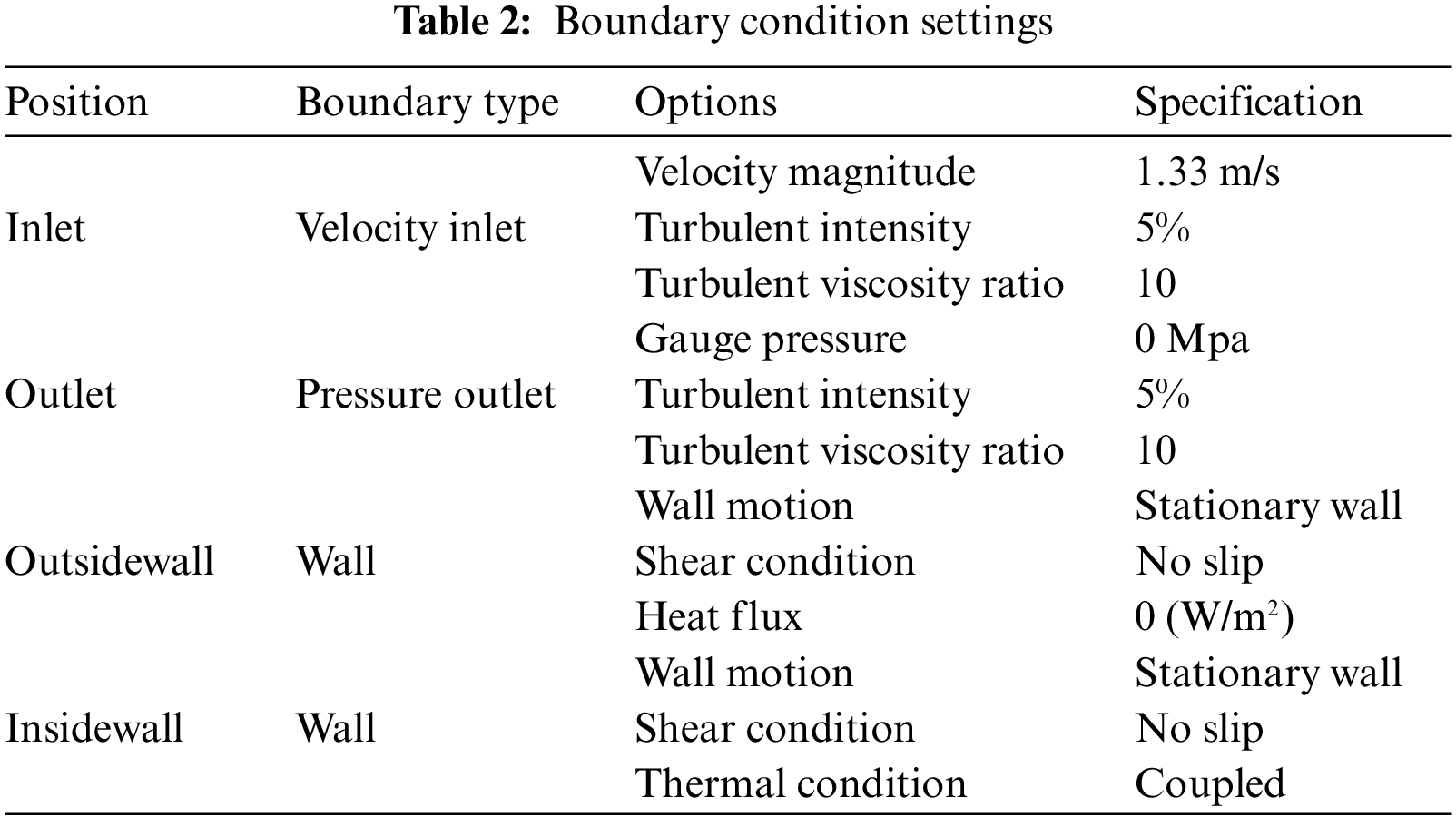
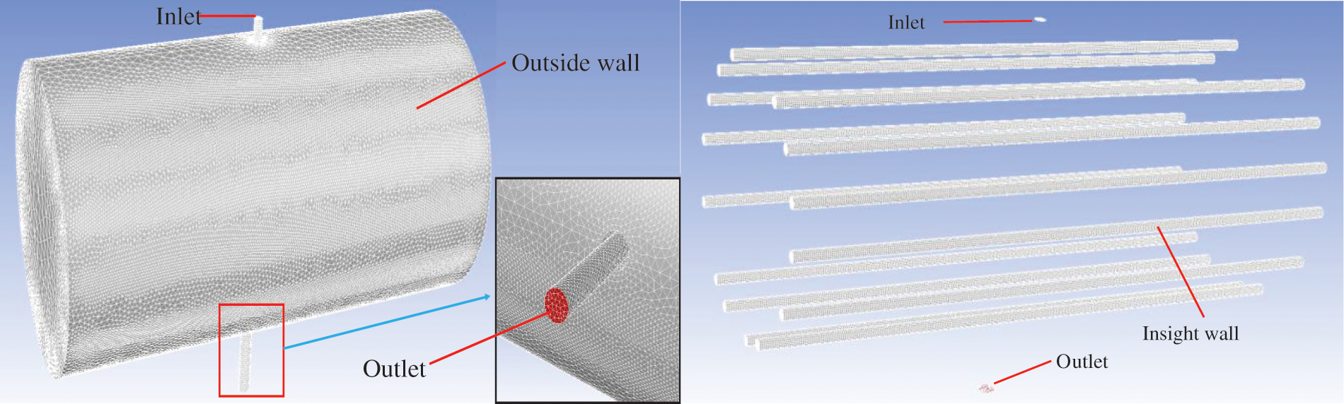
Figure 7: Simulation model boundary of pressure sintering furnace
Based on the simulation model and parameter settings above, the simulation dataset of the sintering furnace is obtained via co-simulation of the flow field and thermal field. The convergent residual curve is obtained and the temperature nephogram, pressure nephogram and streamline diagram of the axial central profile of sintering furnace are extracted. As shown in Fig. 8, the residual error of the model converges to 1e−3 in 18186 steps; at this time, a temperature characteristic of colder in the upper part and hotter in the lower part of the furnace is demonstrated.
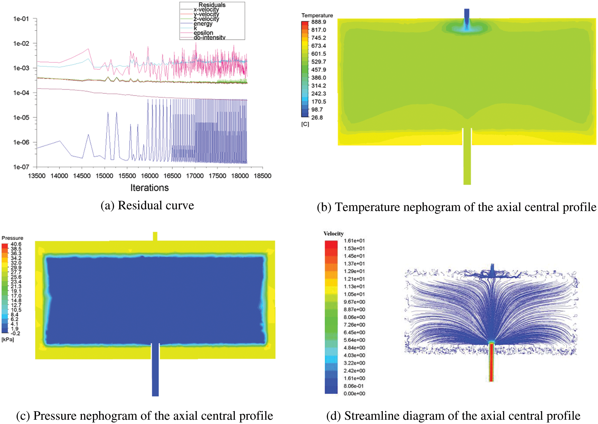
Figure 8: Convergence process and results of pressure sintering furnace simulation
4.1 Sample Extraction Process of Representative Data in Sintering Furnace Simulation
When the temperature in the furnace reaches the temperature required by the process node, the cemented carbide being sintered will be gradually dewaxed to reduce its carbon content. At this point, the temperature distribution in the furnace has a great influence on the quality of cemented carbide dewaxing. In this study, the temperature field data in the furnace are obtained with the proposed data extraction method and process, and the specific process is as follows.
Step 1: Create a candidate direction set. The 3D spatial coordinate system is established by taking the spatial center point of the sintering furnace simulation dataset as the origin, and the candidate direction set
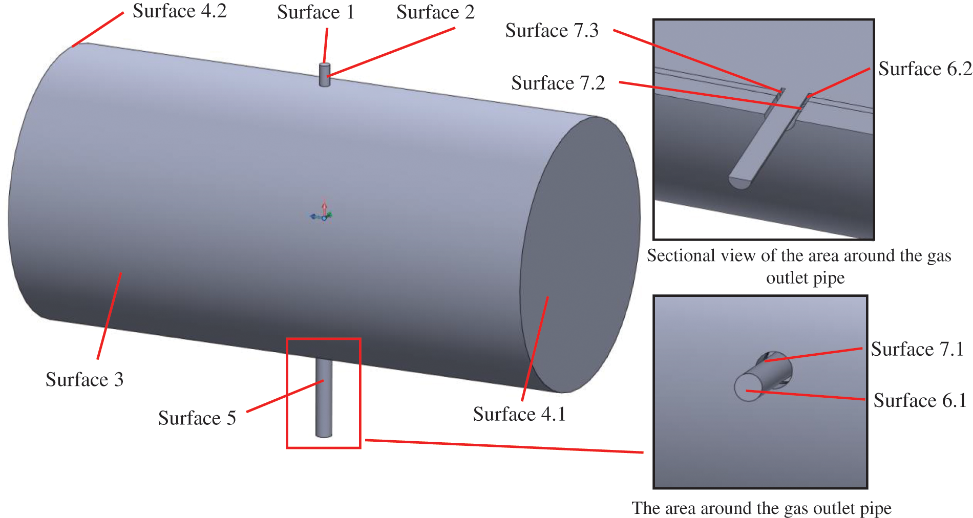
Figure 9: Spatial surfaces of sintering furnace simulation dataset
Similarly, Surface 3, Surface 5 and Surface 7 can be established. Typical directions different from other surface normal vector directions can be selected from their respective spatial normal vector sets. All candidate directions are shown in Table 3.
Step 2: Determine the characteristic direction. The unit normal vector of each dataset surface obtained above is weighted by surface area to obtain the area-weighted normal vector
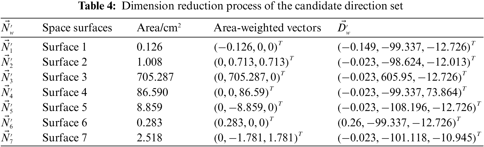
According to formula (10), the covariance matrix
In which,
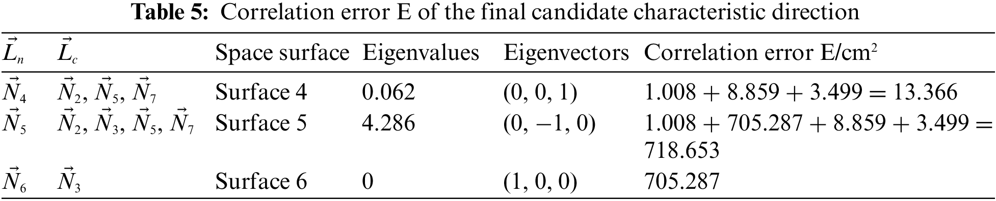
The eigenvalues and eigenvectors of the covariance matrix C are calculated, the three main characteristic directions
Step 3: Initialize the data extraction parameters. Given the similarity and universality in the process of determining data extraction micro-step length by fireworks algorithm optimization, only the first round optimization of fireworks algorithm optimization in the initial optimization interval is taken as an example to demonstrate the data extraction process. Set Surface 4 as the initial dataset A and take the characteristic direction
In view of the difficulty in extracting all data point information from the profile micro-dataset, X data points evenly distributed in profile micro-dataset have been randomly selected to characterize the whole profile micro-dataset in the current study, as shown in Fig. 10. To determine the reasonable number X of sampling points, two uniformly distributed profile micro-datasets have been randomly selected. The correlation R has been calculated according to the gradual change on the number of sampling points in Table 6. When the number of sampling points exceeds 600, the range of fluctuation between the correlations R of the two profile micro-datasets does not exceed 5%. It can be considered that the calculated correlation is independent from the number of sampling points. Hence the number X of sampling points of profile micro-datasets in the process of optimization can be set as 600.
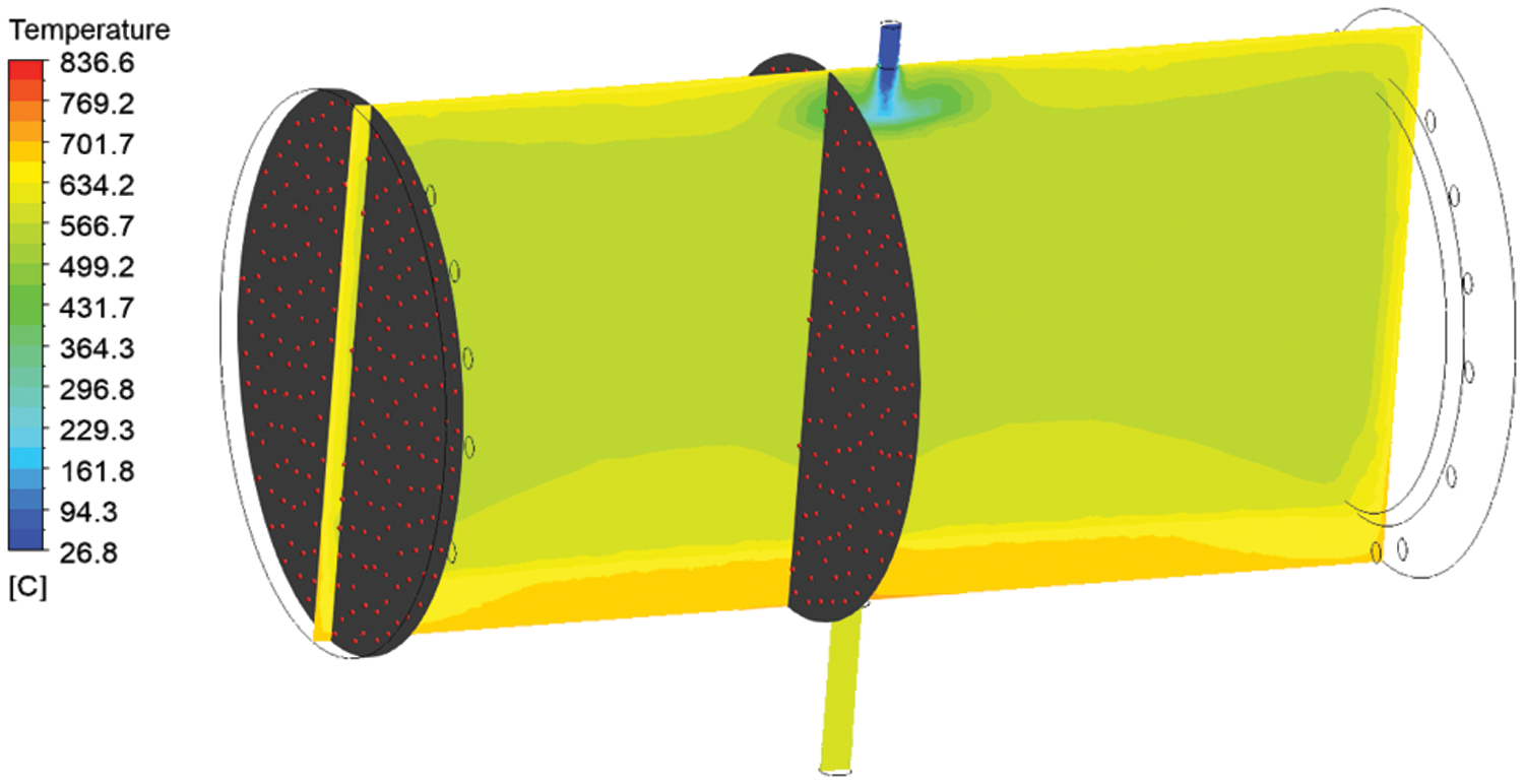
Figure 10: Random sampling point distribution of profile micro-dataset

Step 4: Determine the interval to be optimized. The range of initial optimization interval is set as
Step 5: Determine the termination conditions of data sample extraction. As long as the spatial range of simulation dataset does not exceed the initial optimization interval, the optimization will continue.
Step 6: Fireworks algorithm optimization. The fitness function

When the explosion parameters of each fireworks point are obtained, the specific position and fitness function value
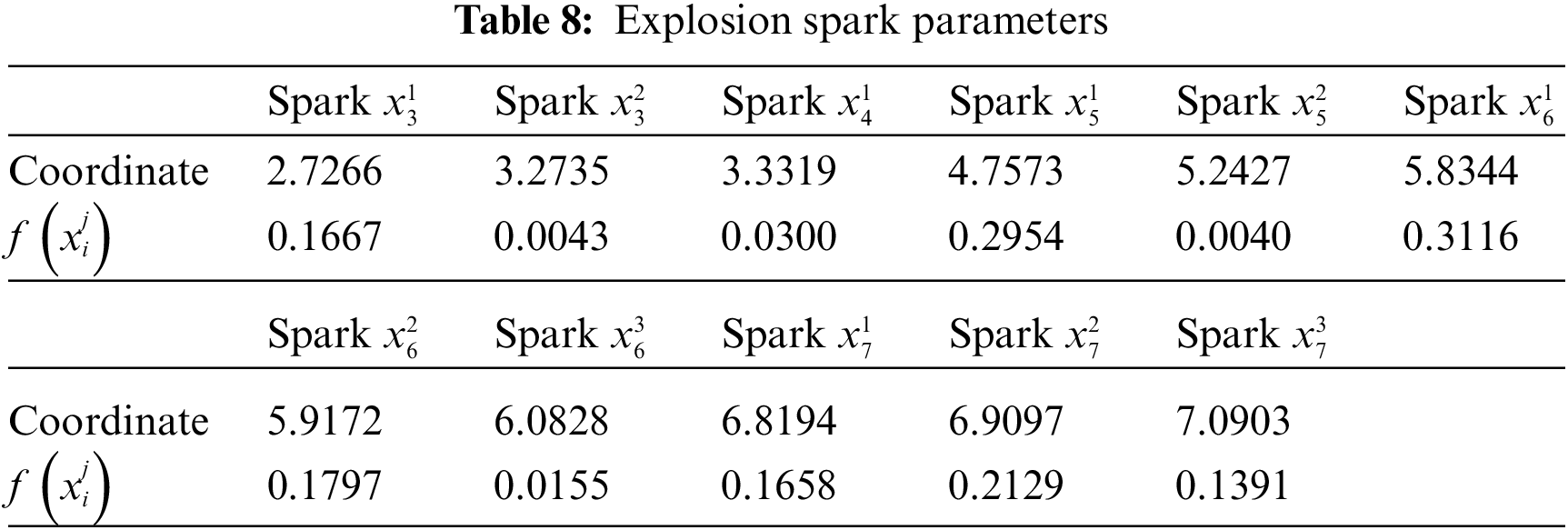
The minimum
Step 7: Determine the termination condition of optimization. As the number of iterations T = 1 <

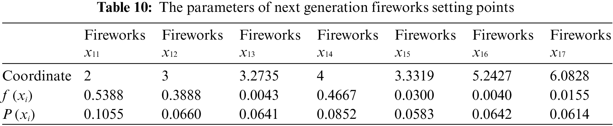
After the setting points of the next generation fireworks are obtained, the optimization process of Step 6 is repeated. The minimum
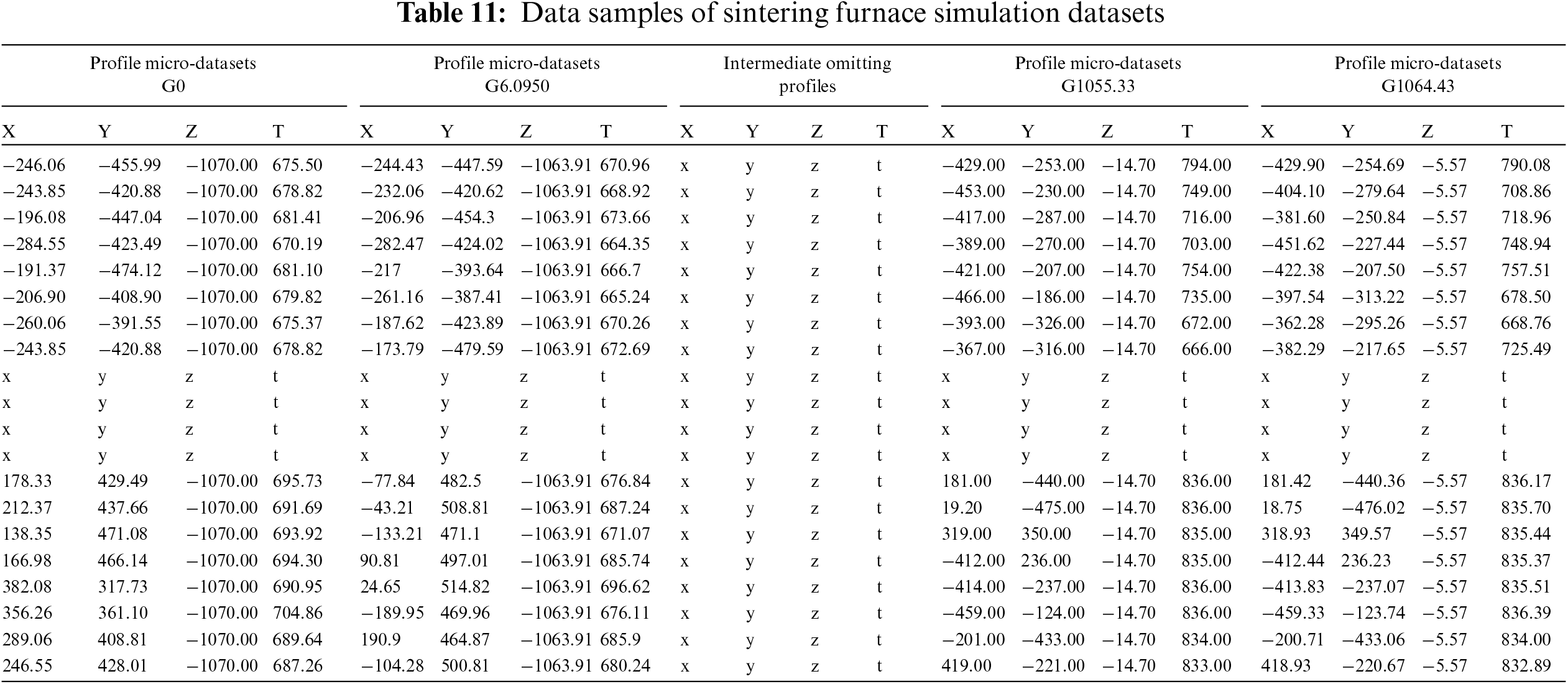
The last extraction interval to be optimized is determined as beyond the range of the sintering furnace simulation dataset and thus the data extraction process of the sintering furnace simulation data sample is considered completed. The final dataset samples of the sintering furnace simulation are shown in Table 11. The data samples are composed of 35 profile micro-datasets, each containing the coordinates and temperature information of 600 data points. To save space, Table 11 only exhibits part of the data samples.
The variation trend of micro-step length along with sampling profile micro-datasets is showed in Fig. 11. The initial sampling area of the sintering furnace dataset is near the furnace door, and the temperature field changes acutely, which leads to small micro-step length. Then the sampling gradually approaches the furnace body and the temperature field tends to be stable, resulting in gradual increase and stability of micro-step length. Finally, the sampling area is near the inlet, and micro-step length demonstrates a rapid decrease as a result of sharp change of the temperature field. By analysis, the variation of the micro-step length of the algorithm is consistent with that of the simulation temperature field, and the expected effect of data sampling has been achieved.
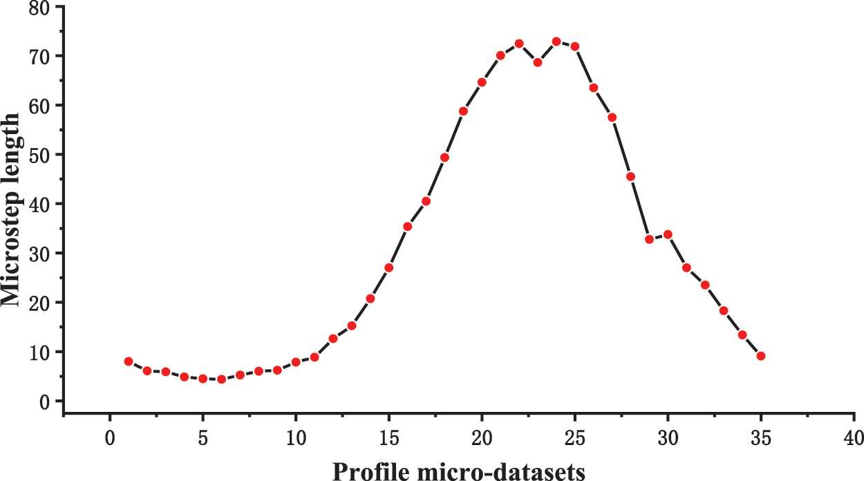
Figure 11: Trend of micro-step length changing with sampling profile micro-datasets
4.2 Validation of Data Samples
An accurate approximation model of the sintering furnace temperature field can be constructed with highly representative and complete simulation data samples. Deploying approximation model, a mathematical model meeting the accuracy and computational efficiency requirements based on limited experimental data can be constructed, which can be utilized to simulate the input-output relations of complex problems. Comparative studies on commonly-used approximation models have demonstrated that radial basis function neural network model has high prediction accuracy and robustness under large sample size, with high computational efficiency of model construction and prediction. It is applicable to highly nonlinear approximate problems with accuracy, and has been widely used in engineering product optimizations [33–35]. In the current study, two radial basis function approximation models
Conventional multi-field co-simulation data extraction methods mainly rely on the selection of multiple equal-distance spatial profiles of field dataset to extract the simulation data sample. The simulation datasets control samples extracted in this fashion are shown in Table 12. The data samples are composed of 43 profile micro-datasets. The distance between each profile micro-datasets is 25 mm, and each profile micro-datasets also contains the coordinate and temperature information of 600 data points. To save space, Table 12 only demonstrates part of the data samples.
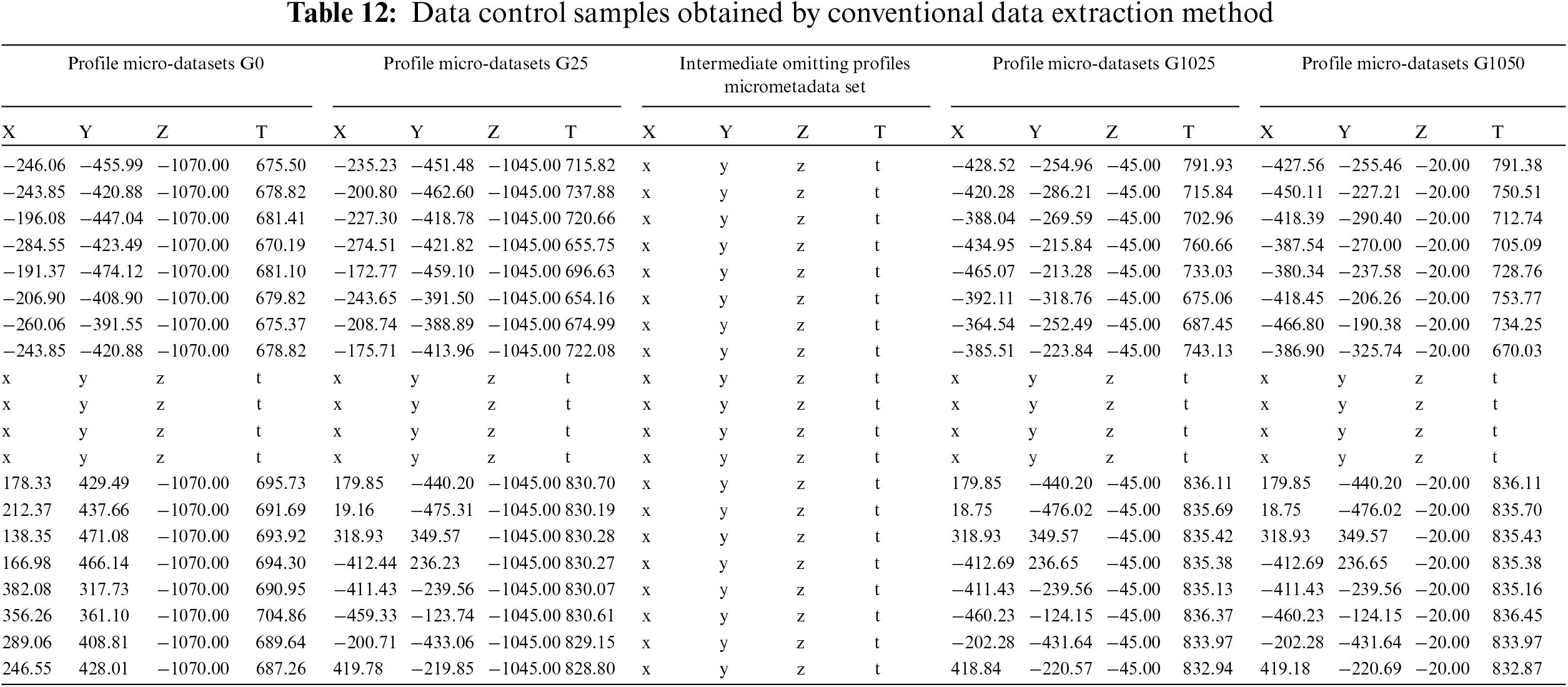
Tables 11 and 12 are the data samples extracted by the proposed data extraction method and data control samples obtained by the conventional data extraction method, respectively. The data control samples are composed of 43 profile micro-datasets, and the distance between each profile micro-datasets is fixed, which leads to inefficient data processing and data duplication; However, the data samples are composed of 35 profile micro-datasets, and the distance between each profile micro-datasets varied according to the characteristics of temperature field, which results in efficient data processing and outstanding data representativeness and diversity.
In general, data points less than 1/3 of the original sample number are selected as verification data to verify the accuracy of the approximation model [36–38]. In the current study, the accuracies of approximation models

The accuracy of the approximation model can be verified by three indicators: relative maximum absolute error (RMAE), root mean square error (RMSE), and coefficient of determination (R2). The mathematical expressions of the three indicators are shown in formulas (18)–(20).
In which, N is the number of verification points;
RMSE is utilized to characterize the dispersion of samples. The closer the RMSE value is to 0, the higher the accuracy of the approximate model is.
R2 is used to characterize the agreement between the predicted value and the real value. The closer the R2 value is to 1, the higher the accuracy of the approximation model is.
In this study, approximation models

Aiming at the limitations of the multi-field co-simulation data extraction method, a multi-field co-simulation data extraction method based on adaptive infinitesimal elements is proposed in the current study. Two points are newly-introduced: First, a characteristic direction determination method based on principal component analysis with the candidate directions in the candidate characteristic direction set dimension-reduced for efficient profile direction selection; Second, an adaptive micro-step length determination method based on the fireworks algorithm in which reasonable number and position of profiles are selected by constantly adjustment on the optimization interval range according to the characteristics of the data. This proposed method has been successfully applied to the data extraction process of the multi-field co-simulation dataset of the sintering furnace. Compared with conventional data extraction methods, the proposed method has exhibited higher data extraction efficiency and accuracy.
In future studies, the adaptive simulation data extraction process for complex multi-surfaces will be focused on, with further explorations into the adaptability and influence of the extracted data samples to different approximation models and optimization algorithms.
Acknowledgement: The authors would like to thank the anonymous reviewers and the editors of the journal. Your constructive comments have improved the quality of this paper.
Funding Statement: This work is supported by the National Natural Science Foundation of China (No. 52075350), the Major Science and Technology Projects of Sichuan Province (No. 2022ZDZX0001) and the Special City-University Strategic Cooperation Project of Sichuan University and Zigong Municipality (No. 2021CDZG-3).
Author Contributions: The authors confirm contribution to the paper as follows: study conception and design: Changfu Wan, Wenqiang Li; analysis and interpretation of results: Sitong Ling, Yingdong Liu; draft manuscript preparation: Jiahao Chen. All authors reviewed the results and approved the final version of the manuscript.
Availability of Data and Materials: The data that support the findings of this study are available from the corresponding author upon reasonable request.
Conflicts of Interest: The authors declare that they have no conflicts of interest to report regarding the present study.
References
1. Nishimi, T., Sato, Y., Kajihara, S., Yoshiyuki, N. (2018). Good die prediction modelling from limited test items. 2018 IEEE International Test Conference in Asia (ITC-ASIA 2018), pp. 115–120. Harbin, IEEE. [Google Scholar]
2. Dri, E. A., Peretti, G. M., Romero, E. A. (2021). A low-cost test strategy based on transient response method for embedded reconfigurable filters. International Journal of Electronics, 19(6), 664–683. [Google Scholar]
3. Komurka, V. E., Theiss, A. G. (2018). Savings from testing the driven-pile foundation for a high-rise building. International Foundations Congress and Equipment Expo 2018, 11, 87–101. [Google Scholar]
4. Sun, H. B., Li, W. Q., Zheng, L. J., Ling, S. T., Wan, C. F. (2022). Adaptive co-simulation method and platform application of drive mechanism based on fruit fly optimization algorithm. Progress in Nuclear Energy, 153, 104397. [Google Scholar]
5. Wei, C., Kang, H. T. (2020). Fatigue life prediction of spot-welded joints with a notch stress approach. Theoretical and Applied Fracture Mechanics, 106, 102491. [Google Scholar]
6. Leung, M., Corcoran, J., Cawley, P., Todd, M. D. (2019). Evaluating the use of rate-based monitoring for improved fatigue remnant life predictions. International Journal of Fatigue, 120, 162–174. [Google Scholar]
7. Amiri, M. (2019). Fatigue life prediction of rivet joints. Journal of Failure Analysis and Prevention, 19(6), 1844–1852. [Google Scholar]
8. Loupy, G. M., Barakos, G. N., Taylor, N. J. (2018). Multi-disciplinary simulations of stores in weapon bays using scale adaptive simulation. Journal of Fluids and Structures, 81, 437–465. [Google Scholar]
9. Yan, X. F., Yan, G. L., Xu, H. J. (2014). A review of virtual prototyping technology for complex electromechanical systems. Computer Integrated Manufacturing Systems, 20(11), 2652–2659. [Google Scholar]
10. Zhou, Y., Tan, Y. X. (2011). Simulation of nine-spacer nozzle’s flow field of Al roll-casting using coupled fluid-thermal finite element analysis. Advanced Materials Research, 159, 697–702. [Google Scholar]
11. Sun, H. B., Li, W. Q., Yu, T. D., Liu, Y. T., Zhang, Z. Q. (2021). Research on associated motion simulation method and platform of control rod driving mechanism. Advances in Mechanical Engineering, 13(9), 1–16. [Google Scholar]
12. Deng, Q., Peng, H., Xie, X. M., Zhang, Z. F., Tang, Y. et al. (2019). Dynamic analysis of control rod driving mechanism based on multi-disciplinary collaborative simulation. Nuclear Power Engineering, 40, 78–81. [Google Scholar]
13. Ling, S. T., Li, W. Q., Zheng, L. J., Li, C. X., Xiang, H. (2022). Flow field fusion simulation method based on model features and its application in CRDM. Nuclear Science and Techniques, 33(3), 89–102. [Google Scholar]
14. Ying, A., Narula, M., Zhang, H., Abdou, M. (2008). Coupled transient thermo-fluid/thermal-stress analysis approach in a VTBM setting. Fusion Engineering and Design, 83(10–12), 1807–1812. [Google Scholar]
15. Luo, D., Wang, R. C., Yan, Y. Y., Sun, Z. Y., Zhou, W. Q. et al. (2021). Comparison of different fluid-thermal-electric multiphysics modeling approaches for thermoelectric generator systems. Renewable Energy, 180, 1266–1277. [Google Scholar]
16. Maher, A., Sadiq, A. B., Muhannad, A. W. (2021). Three-dimensional fluid-thermal-structure multiphysics interaction simulation model of aluminium extrusion process. Journal of Mechanical Engineering and Sciences, 15, 8253–8261. [Google Scholar]
17. Li, N., Xu, H. (2021). Fluid-thermal-structural characteristics of spiral square channel. Journal of Thermal Science and Engineering Applications, 13(3), 031008. [Google Scholar]
18. Ko, S. H., Han, S., Kim, J., Kim, C., Moon, J. B. et al. (2009). Integrated rocket simulation of internal and external flow dynamics in an e-science environment. Journal of the Korean Physical Society, 55(5), 2166–2171. [Google Scholar]
19. Daorina, B., Wang, X. X., Shang, W., Liu, Y. D. (2018). Numerical simulation of flow field in umbrella wind turbine. IOP Conference Series: Earth and Environmental Science, vol. 153, no. 5, 052062. Guilin, China, IOP Publishing. [Google Scholar]
20. Siregar, Y., Kodama, N., Tanaka, Y., Ishijima, T., Uesugi, Y. (2018). Numerical simulation on thermal plasma temperature field in the torch for different conditions. IOP Conference Series: Materials Science and Engineering, vol. 309, no. 1, 012090. Sumatera Utara, Indonesia, IOP Publishing. [Google Scholar]
21. Du, L., Guo, Y., Jiang, L., Li, Q., Zhao, Z. (2017). Effect analysis of temperature and velocity by different combustion models in foursquare tangential circle boiler based on numerical simulation. AIP Conference Proceedings, vol. 1794, no. 1, 040009. Xi’an, R China, AIP Publishing LLC. [Google Scholar]
22. Antonio, G., Norberto, F., Luis, I. D. (2008). Modelling and simulation of fluid flow and heat transfer in the convective zone of a power-generation boiler. Applied Thermal Engineering, 28(5–6), 532–546. [Google Scholar]
23. Wang, C. S., Zhou, Y., Liang, Z. J., Yang, F. X. (2019). Heat transfer simulation and thermal efficiency analysis of new vertical heating furnace. Case Studies in Thermal Engineering, 13, 100414. [Google Scholar]
24. Zhang, S. F., Wen, L. Y., Bai, C. G., Chen, D. F. (2009). Analyses on 3-D gas flow and heat transfer in ladle furnace lid. Applied Mathematical Modelling, 33(6), 2646–2662. [Google Scholar]
25. Abbassi, A., Khoshmanesh, K. H. (2008). Numerical simulation and experimental analysis of an industrial glass melting furnace. Applied Thermal Engineering, 28(5–6), 450–459. [Google Scholar]
26. Wan, C. F., Li, W. Q., Ling, S. T., Liu, Y. D., Chen, J. H. (2022). Multi-scenario group decision-making based on TOPSIS for deep hole drill parameter optimization. Arabian Journal for Science and Engineering, 47(12), 15779–15795. [Google Scholar]
27. Dolenc, A., Makela, I. (1994). Slicing procedures for layered manufacturing techniques. Computer-Aided Design, 26(2), 119–126. [Google Scholar]
28. Ben, E., Saul, F., Gershon, E. (2018). Volumetric covering print-paths for additive manufacturing of 3D models. Computer-Aided Design, 100(5), 1–13. [Google Scholar]
29. Jolliffe, I. T. (1986). Principal component analysis. New York: Springer-Verlag. [Google Scholar]
30. Bishop, C. M. (2006). Pattern recognition and machine learning. New York: Springer-Verlag. [Google Scholar]
31. Tan, Y., Zhu, Y. (2010). Fireworks algorithm for optimization. International Conference on Swarm Intelligence, pp. 355–364. Berlin, Heidelberg, Springer. [Google Scholar]
32. Li, J., Tan, Y. (2019). A comprehensive review of the fireworks algorithm. ACM Computing Surveys (CSUR), 52(6), 1–28. [Google Scholar]
33. Xie, Y., Li, W., Yu, T., Deng, C. J., Hu, X. F. (2020). Research on optimization design of PWR flow distribution device based on numerical simulation. Journal of Nuclear Science and Technology, 57(9), 1074–1090. [Google Scholar]
34. Hardy, R. L. (1971). Multiquadric equations of topography and other irregular surfaces. Journal of Geophysical Research, 76(8), 1905–1915. [Google Scholar]
35. Xiao, M. (2012). Research on approximation models and decomposition strategies in multidisciplinary design optimization. Wuhan, China: Huazhong University of Science and Technology. [Google Scholar]
36. Meckesheimer, M., Booker, A. J., Barton, R. R., Simpson, T. W. (2002). Computationally inexpensive metamodel assessment strategies. AIAA Journal, 40(10), 2053–2060. [Google Scholar]
37. Meckesheimer, M. (2001). A framework for metamodel-based design: Subsystem metamodel assessment and implementation issues. USA: The Pennsylvania State University. [Google Scholar]
38. Andres, E., Salcedo-Sanz, S., Monge, F., Perez-Bellido, A. M. (2012). Efficient aerodynamic design through evolutionary programming and support vector regression algorithms. Expert Systems with Applications, 39(12), 10700–10708. [Google Scholar]
Cite This Article
 Copyright © 2024 The Author(s). Published by Tech Science Press.
This work is licensed under a Creative Commons Attribution 4.0 International License , which permits unrestricted use, distribution, and reproduction in any medium, provided the original work is properly cited.
 Downloads
 Citation Tools