Calculation of Mass Concrete Temperature Containing Cooling Water Pipe Based on Substructure and Iteration Algorithm

1  Introduction

The solutions of partial differential equations have been widely used in civil engineering. It helps engineers take appropriate measures when solving engineering problem. The cooling water pipes are one of the common measures to control concrete temperature in mass concrete construction. When solving the temperature field of this physical phenomenon, Fourier equation needs to consider the hydration heat release of concrete, the change of water temperature along the cooling water, the heat transfer process between cooling water and concrete, and the small grid effect of cooling water pipe (The size of the water pipe is usually measured in centimeters, while the size of concrete is typically measured in meters. As a result, calculating large concrete structures with cooling water pipes can be inefficient due to the mismatch in dimensional units). The essence of solving these problems can be started from the three kinds of boundary conditions of the Fourier equation and the stiffness equation of the finite element method.

The temperature characteristics of concrete can be described using the adiabatic temperature rise. The adiabatic temperature rise of concrete refers to the process of temperature increase in concrete during the curing process, due to the exothermic reaction between cement and water. This process occurs under adiabatic conditions, meaning that the temperature increase within the concrete is solely dependent on the rate of the cement hydration reaction and the heat capacity of the concrete itself. According to experience, the thermal stress generated by hydration heat of cement has a significant impact on the cracks of concrete structures, and 80% of the cracks in mass concrete appear during the construction period [1]. For example, the cracks in the lock head of ship lock generally appear in the area near the side pier of the middle bottom plate, the area near the corner of the corridor, the opening area of the lock and the area with sudden change in shape (valve chamber, water transmission valve bearing beam, etc.). Cracks in the ship lock chamber mainly occur at the bottom of the side wall near the bottom plate and the middle of the bottom plate [2,3].

The existing research on crack prevention and crack resistance of mass concrete mainly starts from three aspects: material selection, structural design, and construction control [4]. In terms of material selection, it is always the ideal choice of concrete to optimize the raw materials and the concrete mix ratio to make concrete have higher tensile strength, smaller adiabatic temperature rise, greater tensile deformation capacity and smaller thermal expansion coefficient [5]. Appropriate addition of fly ash, slag, and other mixed materials to replace cement, adding concrete admixture such as water reducing agent, retarder, air entraining agent, and early strength agent can improve the performance of concrete under the condition of ensuring strength and slump [6,7]. Using a low cement content (178–223 kg/m3) and water cement ratio of 0.6–0.8 can effectively reduce the total calorific value of concrete. In terms of structural design, thin-walled concrete structures and large-sized concrete pouring blocks are prone to cracks, which should be avoided during construction. Concrete pouring blocks should avoid significant undulations and stress concentrations. In terms of construction control, standardized construction processes will significantly improve the quality of concrete. When layered pouring, the concrete pouring blocks should be thin, the construction interval should be short, and the concrete blocks should be poured evenly. Concrete maintenance measures and thermal insulation measures in cold areas should be appropriate. In terms of research on temperature control measures during the construction of mass concrete, engineers have successively put forward temperature control measures such as improved additives, aggregate cooling, thermal insulation transportation, cooling water pipes, surface insulation measures, and jump warehouse construction method.

The gradient of mass concrete temperature produces thermal stress. In previous research shows that the concrete thermal properties are only slightly affected by age, curing condition [8,9]. In addition, as heat transfer analysis is not strongly affected by specific heat and thermal conductivity, the average values for specific heat and thermal conductivity specified by ACI Committee 207 were adopted [10]. As one of the primary measures taken during the construction of mass concrete structures, cooling water pipes has become a topic of extensive research by scholars [11,12]. American engineers took the lead to apply it in the construction processes of arch dams and other hydraulic structures, and greatly reduced the heat dissipation time of the internal temperature of concrete, shortening the construction period. At present, many methods have been formed in the numerical simulation of cooling water pipes, such as direct simulation method, equivalent algorithm, mathematical analysis method, pseudo three-dimensional method, decoupled finite element method for solving water temperature, coupling method for solving water temperature, composite element method, meshless method, radial basis collocation method, etc. The equivalent algorithm focuses on using a large-scale model to equivalent the average cooling effect. This method is mostly based on empirical formulas. The cooling water pipes are regarded as the first or third type of boundary condition, and the cooling effect is considered by imposing boundary conditions. This method is simple to calculate and is mostly suitable for large-scale project calculations. The mathematical analytical method is mainly based on the isotropic assumption to directly solve the standard shapes such as cylindrical concrete or square concrete with cooling water pipes in the center [13]. This method is mainly in the early research work, but limited by various assumptions and model size, there are few research on mathematical analytical method at present [14]. The pseudo three-dimensional method regards the three-dimensional heat transfer problem of cooling water-concrete heat transfer as the plane strain problem to achieve dimension reduction. Under this method, Myers et al. analyzed the influence of pipe material, pipe radius, flow velocity and other parameters on concrete temperature [15,16]. By establishing the energy equation of the contact surface between water pipe wall and concrete, decoupled finite element method for solving water temperature performs the iterative calculation according to these steps. Firstly, the heat of concrete hydration is calculated. Secondly, the heat transfer towards the cooling water pipe is obtained. Thirdly, the heat transfer inside the cooling water pipe is got. Finally, the concrete temperature calculation is finished [17,18]. The coupling method mainly sets the cooling pipes as line elements and calculates the heat transfer processes between the cooling pipes and concrete [19]. The composite element method mainly corresponds to the degree of freedom of concrete elements and cooling water elements, then separates the meshes through geometric information [20]. In addition to the traditional finite element method, a series of scholars have successively carried out simulation research on the temperature field of concrete with cooling water pipes using the meshless method [21,22]. The embedded element method is used to simulate the cooling pipe, analyzed the influence of the convection coefficient at the boundary of the cooling pipe, and improved the calculation method of water temperature along the cooling pipes [23]. The radial basis collocation method uses the linear combination of radial basis functions to approximate the physical quantity. The matrix formed by this method has better positive definiteness and a smoother solution. Since the radial basis function is only related to the distance between the configuration points, it has nothing to do with the exact location of the configuration points. Therefore, it can be easily extended to high-dimensional spaces [24]. Hong et al. optimized the constant flow of the cooling water pipe, which effectively improved the safety of the structure and the economy of construction [25].

In fact, the temperature field of concrete with cooling water pipes is constantly changing on the spatial and temporal scales, and these changes have a new impact on the water temperature in the cooling water pipes. Although the direct simulation method can intuitively simulate the temperature changes of cooling water flow, cooling water pipes (plastic or metal), and concrete, there are two problems in the calculation process of the combined model: First, the scale of the model is different. It is difficult to unify the large-scale concrete model and the small-scale cooling water pipe model on the finite element grid, resulting in a large number of grids. Second, the iteration numbers of the temperature within a time step at the inner boundary of the water pipe will directly affect the calculation efficiency. The in-depth study of Qiang et al. [26] pointed out that a compo-site element coupled with water and concrete can be used to replace the concrete element with cooling water pipes, so as to make up for the time-consuming calculation caused by the first factor mentioned above. Based on this idea, this paper adopted the substructure method to solve the concrete in the area containing cooling water pipes. The iteration times of boundary temperature equilibrium between cooling water and cooling water pipe are shortened by the method of external control iteration. The results of the classical model are used to test the calculation method in this paper.

2  Calculation of Mass Concrete Temperature Containing Cooling Water Pipe Based on Iteration Algorithm

The heat of concrete is rapid after pouring, and its heat conduction equation is as follows [27]:

∂T∂t=λρc(∂2T∂x2+∂2T∂y2+∂2T∂z2)+∂Qθ∂t(1)

where: λ is the thermal conductivity of concrete, c is the heat capacity of concrete, ρ is the density of concrete, and Qθ is the heat of hydration of concrete.

The cooling water pipes are often adopted in the construction of mass concrete. The heat flow transferred between concrete and water pipe boundary can be expressed as [28]:

q=−λg∂T∂n(2)

where: λg is the thermal conductivity of water pipe; T is the temperature of concrete. The heat transferred from the pipe wall to the water flow per unit time can be expressed as the area integral between the heat flow and the pipe wall:

Qc=−λg∬S∂T∂nds(3)

When the water temperature in the cooling water pipe changes along the way, the heat change of the cooling water per unit length per unit time can be expressed as:

Qchf=qwρwcw(Tout−Tin)(4)

where: qw is the water flow rate; ρw is the water density; cw is the specific heat of water; Tout is the water temperature at the outlet; Tin is the water temperature at the inlet; Qchf is the heat taken away by cooling water per unit time.

By combining (3) and (4), the following is obtained from the conservation of energy:

Tout=Tin−λgqwρwcw∬S∂T∂nds(5)

Then, the recursive formula of the water temperature of the cooling water pipe is obtained. The formula shows that the cooling water temperature is a variation related to the water flow rate, the material of the cooling water pipe, the area of the cooling water pipe, the thickness of the cooling water pipe and the temperature of the adjacent concrete. For the cooling water pipe area with a unit width (as shown in Fig. 1), the temperature equilibrium equation can be obtained from (5) as follows by us:

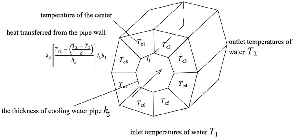
Figure 1: Finite element diagram of cooling water pipe

qwρwcw(T2−T1)=∑i=18λg[Tci−(T2+T12)hg]libi(6)

where: T2 and T1 are the outlet and inlet temperatures of water flowing through the unit; Tci is the center temperature of each element; li, bi is the length and width of the boundary between the adjacent concrete and the water pipe; hg is the thickness of cooling water pipe; λg is the thermal conductivity of water pipe material. By converting (6) into an explicit equation about outlet temperature T2, we can obtain:

T2=ρwcwqwT1+λg2hg∑i=18(2Tci−T1)libiρwcwqw+λg2hg∑i=18libi(7)

In the above equation, the centroid temperature of the adjacent concrete and the outlet temperature of the water flow are unknown variables. Since the temperature of the cooling water pipe and the boundary of concrete presents nonlinear changes, the iterative solution method can be used to gradually approach the real solution. In one solution step, firstly, assuming that the temperature along the cooling water pipe is constant and equal to the inlet temperature, the concrete temperature field is calculated, and then the temperature along the cooling water pipe is calculated by the inlet temperature and Eq. (6). The temperature of concrete and cooling water pipe tends to be stable by repeating this process. The specific implementation steps are as follows:

a)   Assuming that the boundary of the concrete and cooling water pipe is an adiabtic boundary. This means that heat transfer across the boundaries in the first specific implementation step is not allowed. In other words, it is assumed that the cooling water pipe is perfectly insulated from the surrounding water. The purpose of this assumption is to obtain an initial value of the concrete that is higher than the one containing cooling water pipes, which serves as the initial temperature values for the iterative calculation process. The temperature field of the concrete is calculated as the concrete temperature field of the initial iteration step, and the element centroid temperature TΓ1 is derived.

b)   Assuming that the temperature of the cooling pipe is the initial temperature, the temperature field TΓ1 obtained in (a) and Eq. (6) is used to obtain the temperature field TwΓ1.

c)   According to the junction temperature TΓ at the boundary and the temperature field TwΓ1 of the water pipe in (a), the surface heat dissipation qΓ at each boundary is obtained according to Eq. (2).

d)   Fourth item; applying the heat dissipation qΓ in (c) to the boundary of the concrete cooling water pipe in (a), the temperature field of the concrete is recalculated, and the junction temperature TΓ2 at the boundary of the concrete and water pipe is derived again.

e)   Repeating (b)~(d) until the iteration number n is nmax or the updated junction temperature TΓn−TΓ(n−1) at the concrete boundary meets the iteration accuracy ε. Water pipe temperature field and concrete temperature field are output at this time.

The interation algorithm is applied in the temperature convergence. This mathematical problem can be shown as follows. The initial input value is TΓ1. The function TΓn=f(TΓn−1) is the output value, where f is shown the calculation processes of Eqs. (1)~(7). Then the iteration accuracy εn−1=|TΓn−TΓn−1| is calculated. The εn−1<ε is the convergence condition. The iteration algorithm is applied in this paper. It is shown as (8):

TΓn+1=(1−α)TΓn+αTΓn−1(8)

where α is the parameter, the range of α is 0~0.5. By this parameter, a mathematical relationship between the temperature value in the next iteration and the temperature values obtained from the previous two iterations can be established. It can accelerate the iteration process and gradually approach stability.

The diameter of cooling water pipe is usually about 1 to 2 inches, which is much smaller than the size of the concrete structure. The key to simulate the cooling of water pipe is the accurate establishment of the mass concrete model containing cooling water pipe. This is difficult for the meshing of complex structures, but the substructure method can solve the above problems effectively. The substructure method is also known as the super element technology, which divides the complex structure into several small-scale substructures, and each substructure is connected by boundaries. In solving the problem, the common boundary is fixed first, and the stiffness matrix of each substructure relative to the common boundary is calculated. Then, the finite element balance equation is used to assemble the substructure stiffness matrix through the common boundary, and the whole structure balance equation is formed. Finally, the solved common boundary junction temperature is taken as the specified temperature to solve the internal temperature of the substructure.

In the calculation of the concrete temperature field considering the cooling water pipe, the substructure method can be used to isolate the external changes other than the substructure, which can save part of the cost of stiffness calculation. Because the stiffness calculation and structure condensation of the substructure are performed only once, the calculation efficiency is effectively improved. For the problem of cooling water pipes, common cooling water pipe structures include quadrilateral, hexagonal and octagonal water pipes. The schematic diagram of the grid divided according to this is shown in Fig. 2. The internal junction temperature and load of the substructure are {Tg} and {Pg}, and the junction temperature and load at the common boundary are {Tc} and {Pc}. Then the stiffness matrix of the substructure is shown as [29]:

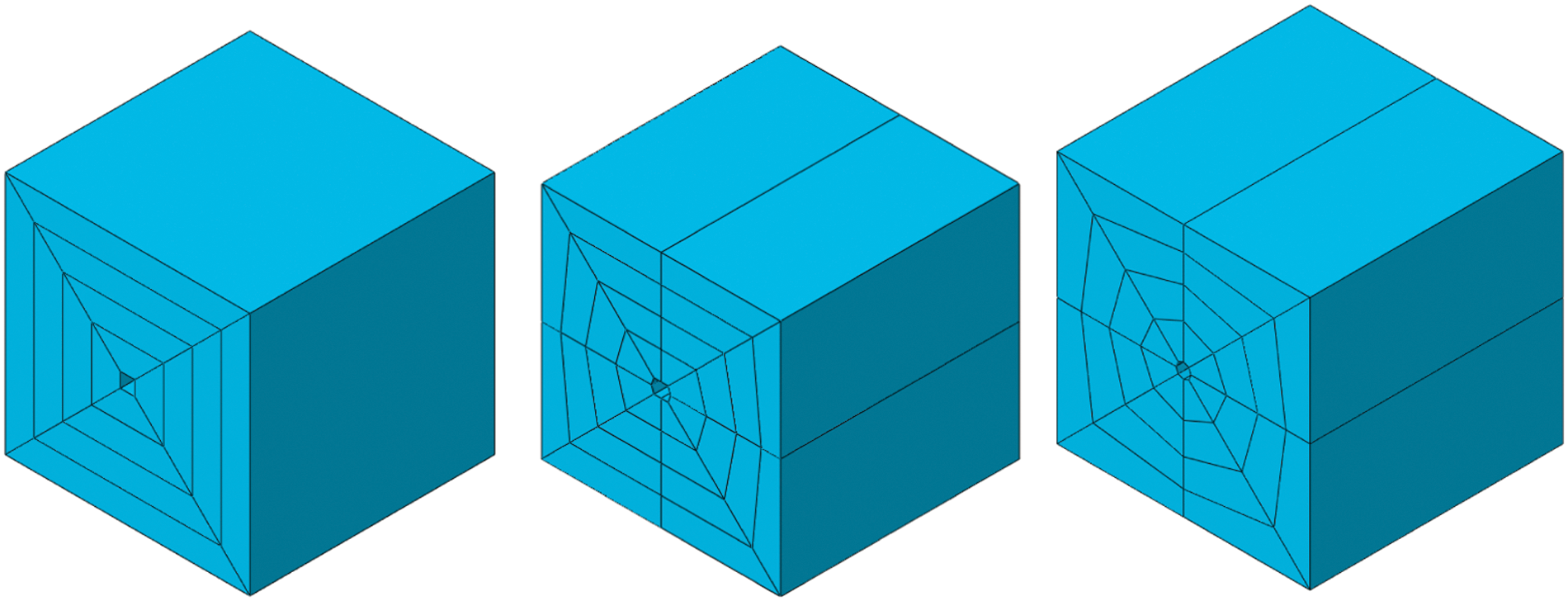
Figure 2: Schematic diagram of the substructure

[KgKgcKcgKc]{TgTc}={PgPc}(9)

After matrix simplification is performed on (9), the stiffness matrix of common boundary junction can be obtained, as follows:

([Kc]−[Kcg][Kg]−1[Kcg])T{Tc}={Pc}−[Kcg][Kg]−1{Pg}(10)

The substructure method has been validated by scholars. In previous research by Liu et al. [29], the authors validated the method through two typical cases. The first case was the cooling problem of an infinitely long cylinder. The author analyzed and validated the theoretical solution and finite element solution of the temperature field of the concrete at representative locations. The second case was the temperature field calculation of a concrete casting block with serpent-shaped cooling water pipes, and the substructure method was validated against the conventional finite element method. Through these two cases, the accuracy of the substructure method in finite element simulation of cooling water pipes was demonstrated. This laid the foundation for the iterative calculation research of cooling water pipes in this paper.

3  Parameter Modeling Calculation Method of Cooling Water Pipe Based on Secondary Development of Abaqus/Python

Through the secondary development of commercial software, the calculation of cooling water pipe is completed by direct modeling, calculation iteration processes. This section takes Abaqus as an example. It can effectively solve the problem of low efficiency of Abaqus/cae pre-processing and post-processing operations based on the secondary development of Abaqus/Python language and make some problems with specific laws can be uniformly solved. For example, when multiple-parts components are assigned attributes in a complex structure model, multiple complex operations can be programmed through Abaqus/Python secondary development for a programming loop, or similar problems can be solved by creating a functional plug-in at once [30]. For another example, in the problems of parameter optimization, sensitivity analysis, and structural optimization design, it is necessary to repeatedly substitute data, modify the model, design algorithms, output results, and set the objective function optimization. These massive calculation processes can also be simplified by Abaqus/Python secondary development [31]. In addition, Python language is concise, easy to learn, high development efficiency, and has powerful module library support.

The theoretical process of cooling water pipe calculation using Abaqus/Python secondary development is the same as in Section 2. The calculation steps are consistent with the Abaqus/cae operation process, and the difficulty lies in the establishment of the model including the cooling water pipe. It mainly includes:

a)   For the establishment of a concrete structure model, the coordinates of structural control points are used to output the solid model. For example, the rectangular solid can be built by:

s.rectangle(point1=rec1_x,point2=rec1_y)

b)   To establish the regional model of the cooling water pipe, input the boundary coordinates of the water pipe and the coordinates of the cutting point in sequence. The coordinates of the latter two can be generated in batches from the water pipe boundary coordinates and control parameters. Using the PartitionCellByPlaneThreePoints function and findAt function of Abaqus to cut refined mesh area in batch, the cross-sectional shape of the entity after cutting refers to Fig. 2.

c)   For the establishment of the unit set and surface set at the boundary between concrete and cooling water pipe, the unit set and surface set at the boundary between concrete and water pipe after cutting are created into individual sets in batches by using cycle variable, find At function and Set function, which are orderly named SG_ele1, 2…,n, SG_upset1, 2…,n, SG_downset1, 2,…,n, SG_leftset1, 2,…,n, SG_rightset1, 2,…,n.

d)   Create an analysis step. Take 1d as the calculation time of the analysis step and assign an initial value of 10°C to each surface set in batches to form an initial iteration model.

e)   Grid division. The refined area containing water pipes is divided into grids, and then other areas are divided to ensure the continuity of nodes.

f)   Submit the .inp file and hydration heat subroutine Hetval.for for calculation. The centroid temperature of each unit in (c) is output in the post-processing, and the water temperature and surface heat flux after iteration are calculated using Eqs. (7) and (4).

g)   Iterative calculation. The surface heat flux in (f) was re-assigned to each surface set, and the calculation was repeatedly submitted until the iteration accuracy was satisfied. The wait function waitForCompletion is set between each submission and the subsequent submission, and one analysis step, namely 1 d temperature iterative calculation, is completed.

h)   Transient calculation of temperature field. Add a new analysis step to the last iteration of the file. The function loads. setValuesInStep was used to modify the surface heat flux in the new analysis step, and the process (f) and (g) was repeated for the iterative calculation of the temperature field in the next 1 d.

4  Method Verification

4.1 Verification of Concrete Temperature Field Containing a Cooling Water Pipe

Literature [29] studied the temperature field of concrete containing a cooling water pipe. The results are verified by the method presented in this paper. There are 3 m × 3 m × 3 m concrete block with an initial temperature of 10°C and a constant bottom temperature of 10°C. The other surface dissipate heat at 10°C. The thermal conductivity coefficient of concrete is 0.1 m2/d, the adiabatic temperature rise function is θ(τ)=25(1−e−0.397τ), the thermal conductivity is 236.81 kJ/(m ● d ● °C), the heat dissipation coefficient is 1184.07 kJ/(m2 ● d ● °C), the cooling water pipe is located in the center of concrete, the diameter is 0.04 m, the inlet water temperature is 3°C, and the flow rate is 21.6 m3/d.

A mass concrete containing a cooling water pipe example is used to verify the feasibility of our method. Fig. 3 shows the main process of calculation, including batch generation and updating of temperature boundaries in Abaqus, batch submission of calculation, and storage of calculation results. The python script can effectively implement the pre and post processing of the calculation and complete the iterative calculation. The file .txt shows the calculation results.

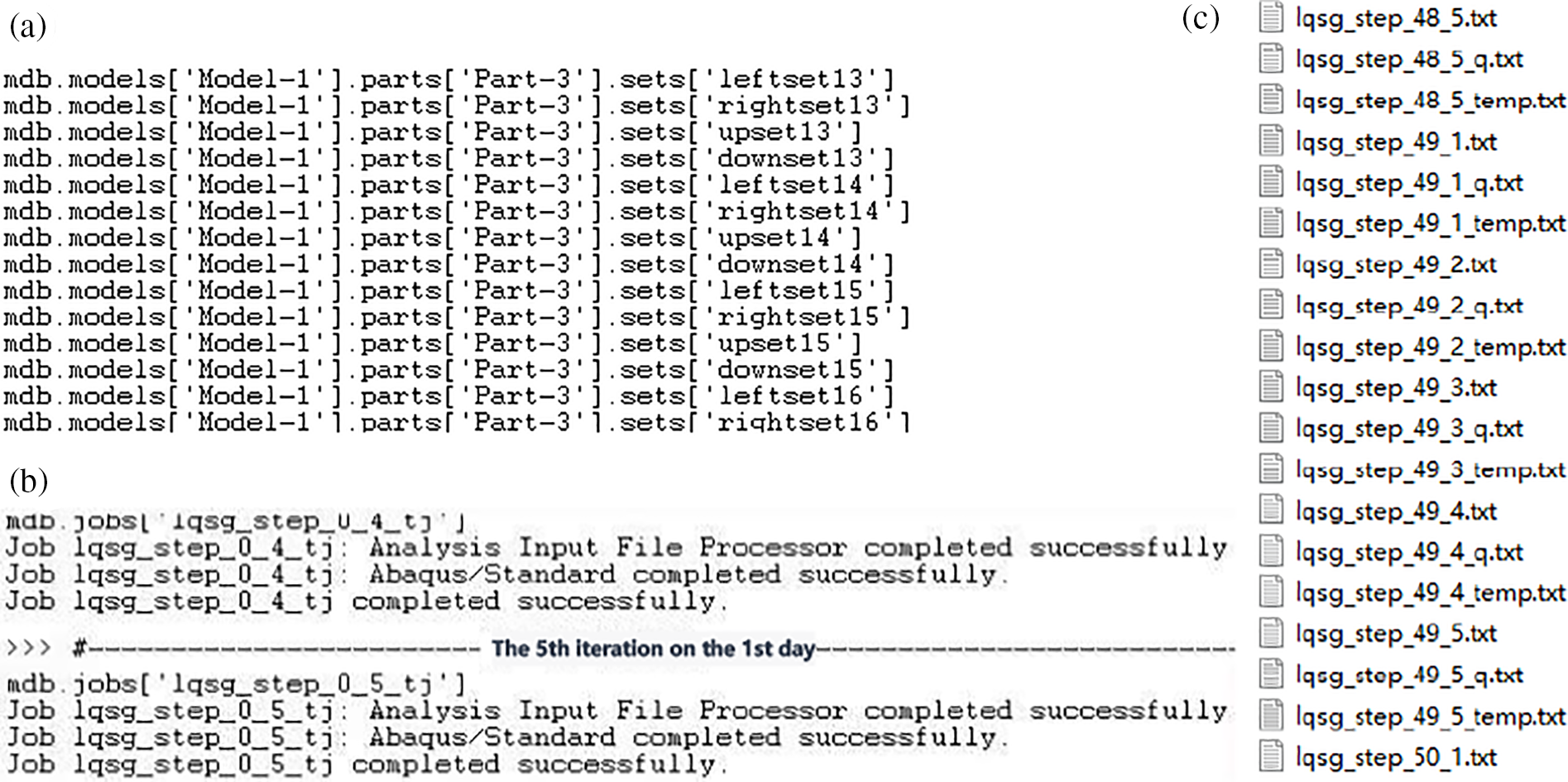
Figure 3: Demonstration of the main process of calculation. (a) Apply the temperature boundary; (b) submit jobs; (c) results

Fig. 4 shows the 10 iterations of temperature at the outlet of the water pipe. In our method, the temperature is stable almost after 3 iterations when α is 0.4. This model provides a reasonable recommended value.

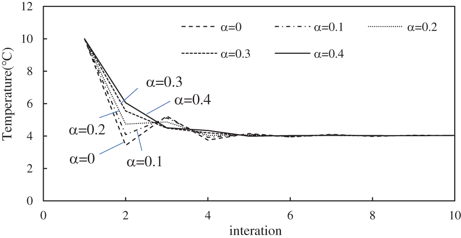
Figure 4: 10 iterations of temperature at the outlet of pipe at 2.5 d

Fig. 5a shows the average temperature at 0.5 m away from the center. The calculation method in this paper is basically the same as the results obtained in the literature. The calculation error of each position shall be controlled within 1.5°C. The temperature changes in a hyperbolic manner. When a single water pipe is used, the maximum temperature at this position reaches 24.6°C on the 2.5 d. The final temperature of the concrete is stabilized at 10°C. Fig. 5b shows the temperature cloud diagram of the center section at 2.5 d. The cooling water pipe has a significant cooling effect on the concrete center. The distribution law is similar to the measured results in some engineering sites [12].

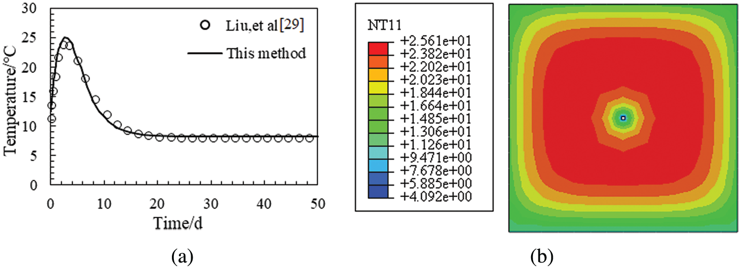
Figure 5: Calculation results. (a) Average temperature at 0.5 m from the center; (b) temperature cloud diagram at the central section at 2.5 d (unit: °C)

4.2 Verification of Temperature Field of Cooling Water Pipe Arranged in a Serpentine Shape

The concrete temperature field of the cooling pipe arranged in a serpentine shape is calculated and verified by the method presented in this paper. The parameters of the concrete and cooling water pipes are the same as in Example a. The position of the serpentine pipe in the concrete middle layer. The cooling pipes are arranged with a spacing of 1 m. Fig. 6 shows the results of concrete calculation meshing with serpentine cooling water pipes. This paper simplified the turning area of water pipe. Fig. 7a shows the average temperature at 0.5 m away from the center. When the water pipes are arranged in a serpentine shape, the maximum temperature at this position reaches 20.0°C on the 2.5 d. The calculation method in this paper is basically the same as the results obtained in the literature. The calculation error shall be controlled within 2°C. Fig. 7b shows the temperature cloud diagram of the central section at 2.5 d. The cooling water pipe can effectively reduce the temperature of the middle layer.

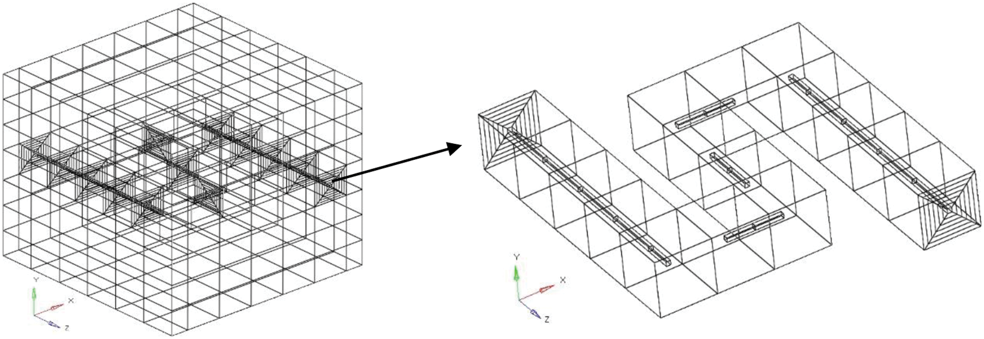
Figure 6: Computational meshing

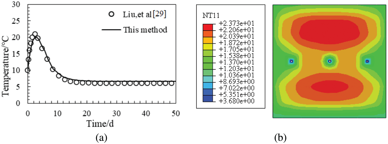
Figure 7: Computational meshing. (a) Average temperature at 0.5 m from the center; (b) temperature cloud diagram at the central section at 2.5 d (unit: °C)

5  Discussions

Simulation research on mass concrete cooling water pipes has always been a hot issue for engineers. In this paper, the substructure method and iterative algorithm are used to solve the temperature field. The substructure method is a method of packaging the stiffness matrix of a repetitive local model and then placing it into the overall stiffness matrix model for calculation, which has the advantages of fast calculation and short time consumption. Using this method can avoid the phenomenon that the model size is large across the grid. This method is introduced into the calculation of concrete temperature with cooling water pipes in this paper.

The temperature calculation method is based on Fourier equation. The heat of hydration, as a heat source term in the equation, is fitted by a commonly used power function heat release curve. This assumption is consistent with literature [12,27]. The innovation of this article is to introduce iterative control parameters into the substructure algorithm based on previous research. The optimal value of the parameter α is determined to be 0.4 through numerical experiments. The substructure method and iterative algorithm successfully solves the problem of low computational efficiency of concrete containing cooling water pipes.

Based on the secondary development of Abaqus/python, the classical models of single distributed and serpentine distributed water pipes are verified. The calculation law of temperature field of mass concrete with cooling water pipes is consistent with the experimental results in literature [29]. The Abaqus plug-in method including pre and post processing of calculations is the same as that used in literature [30,31]. Based on these arguments, the calculation efficiency of the method proposed in this paper can be guaranteed in practical projects. The method proposed in this paper can further simulate the initial temperature of cooling water, the space between cooling pipes, and the cooling pipe material effect on temperature distribution and temperature gradient in subsequent research.

6  Conclusions

In this paper, based on the direct simulation method of the cooling water pipe, combined the substructure technology with the iteration algorithm, a parametric modeling calculation method of the cooling water pipe using Abaqus/Python secondary development is proposed, and the feasibility and accuracy of the method are verified by two numerical examples. The main conclusions are as follows:

(1)   The proposed method combines substructure technology with an iteration algorithm, which significantly reduces the computation time needed for numerical simulations. The proposed method addresses the issue of low computational efficiency in large-scale concrete structure calculations of cooling water pipes caused by inconsistent units of dimension.

(2)   This paper proposes a parametric modeling calculation method for cooling water pipes using Abaqus/Python secondary development, and the verification of test results shows that this method can basically meet the accuracy requirements and the error is small. This numerical simulation method can be well applied on the complex arrangement form, such as serpentine shape cooling pipes.

(3)   This article explores the impact of the α on the number of iterations and provides a recommended value of 0.4. It not only saves computational resources and time but also enhances the accuracy and reliability of the simulations. Therefore, the proposed method has great potential for practical applications in the design and optimization of cooling water pipes.

Acknowledgement: None.

Funding Statement: This work was supported by Construction Simulation and Support Optimization of Hydraulic Tunnel Based on Bonded Block-Synthetic Rock Mass Method and Hubei Province Postdoctoral Innovative Practice Position.

Author Contributions: Study conception and design: H.Z., C.S.; data collection: H.Z.; analysis and interpretation of results: S. Z., C.X.; draft manuscript preparation: H.Z. and H.L. All authors reviewed the results and approved the final version of the manuscript.

Availability of Data and Materials: The data and materials are available upon request.

Conflicts of Interest: The authors declare that they have no conflicts of interest to report regarding the present study.

References

1. Zhang, H. (2022). Study on simulation method of hydraulic structure on soft foundation during construction (Ph. D. Thesis). Hohai University, China. [Google Scholar]

2. Ju, Y., Lei, H. (2019). Actual temperature evolution of thick raft concrete foundations and cracking risk analysis. Advances in Materials Science and Engineering, 2019(5), 1–11. https://doi.org/10.1155/2019/7029671 [Google Scholar] [CrossRef]

3. Sheng, Z. B., Deng, C. L., Xiong, J. B. (2020). Concrete cracking control of chamber wall in jiepai ship-lock project. IOP Conference Series: Earth and Environmental Science, vol. 531, 012043. IOP Publishing. https://doi.org/10.1088/1755-1315/531/1/012043 [Google Scholar] [CrossRef]

4. de Borst, R., van den Boogaard, A. H., (1994). Finite-element modeling of deformation and cracking in early-age concrete. Journal of Engineering Mechanics, 120(12), 2519–2534. https://doi.org/10.1061/(ASCE)0733-9399(1994)120:12(2519) [Google Scholar] [CrossRef]

5. Hover, K. C. (2011). The influence of water on the performance of concrete. Construction and Building Materials, 25(7), 3003–3013. https://doi.org/10.1016/j.conbuildmat.2011.01.010 [Google Scholar] [CrossRef]

6. Kevin, J. F., Neal, S. B. (1997). Properties of high-performance concrete containing shrinkage-reducing admixture. Cement and Concrete Research, 27(9), 1357–1364. https://doi.org/10.1016/S0008-8846(97)00135-X [Google Scholar] [CrossRef]

7. Mohamed, A. K., Weckwerth, S. A., Mishra, R. K. (2022). Molecular modeling of chemical admixtures; opportunities and challenges. Cement and Concrete Research, 156, 106783. https://doi.org/10.1016/j.cemconres.2022.106783 [Google Scholar] [CrossRef]

8. Khaliq, W., Kodur, V. (2011). Thermal and mechanical properties of fiber reinforced high performance self-consolidating concrete at elevated temperatures. Cement and Concrete Research, 41(11), 1112–1122. https://doi.org/10.1016/j.cemconres.2011.06.012 [Google Scholar] [CrossRef]

9. Lim, C. K., Kim, J. K., Seo, T. S. (2016). Prediction of concrete adiabatic temperature rise characteristic by semi-adiabatic temperature rise test and FEM analysis. Construction and Building Materials, 125(5), 679–689. https://doi.org/10.1016/j.conbuildmat.2016.08.072 [Google Scholar] [CrossRef]

10. Payam, S., Iman, A., Norhayati, B. M. (2018). Concrete as a thermal mass material for building applications—A review. Journal of Building Engineering, 19(5), 14–25. https://doi.org/10.1016/j.jobe.2018.04.021 [Google Scholar] [CrossRef]

11. Kim, J. K., Kim, K. H., Yang, J. K. (2001). Thermal analysis of hydration heat in concrete structures with pipe-cooling system. Computers & Structures, 79(2), 163–171. https://doi.org/10.1016/S0045-7949(00)00128-0 [Google Scholar] [CrossRef]

12. Tran, M. V., Chau, V. N., Nguyen, P. H. (2023). Prediction and control of temperature rise of massive reinforced concrete transfer slab with embedded cooling pipe. Case Studies in Construction Materials, 18, e01817. https://doi.org/10.1016/j.cscm.2022.e01817 [Google Scholar] [CrossRef]

13. Tasri, A., Susilawati, A. (2019). Effect of material of post-cooling pipes on temperature and thermal stress in mass concrete. Structures, 20(2), 204–212. https://doi.org/10.1016/j.istruc.2019.03.015 [Google Scholar] [CrossRef]

14. Tasri, A., Susilawati, A. (2019). Effect of cooling water temperature and space between cooling pipes of post-cooling system on temperature and thermal stress in mass concrete. Journal of Building Engineering, 24(4), 100731. https://doi.org/10.1016/j.jobe.2019.100731 [Google Scholar] [CrossRef]

15. Myers, T., Fowkes, N., Ballim, Y. (2009). Modeling the cooling of concrete by piped water. Journal of Engineering Mechanics, 135(12), 1375–1383. https://doi.org/10.1061/(ASCE)EM.1943-7889.0000046 [Google Scholar] [CrossRef]

16. Myers, T., Charpin, J. (2008). Modelling the temperature, maturity and moisture content in a drying concrete block. Mathematics-in-Industry Case Studies, 1, 24–48. [Google Scholar]

17. Singh, P. R., Rai, D. C. (2018). Effect of piped water cooling on thermal stress in mass concrete at early ages. Journal of Engineering Mechanics, 144(3), 25–47. https://doi.org/10.1061/(ASCE)EM.1943-7889.0001418 [Google Scholar] [CrossRef]

18. Sabbagh-Yazdi, S. R., Wegian, F. M., Ghorbani, E. (2008). Investigation of the embedded cooling pipe system effects on thermal stresses of the mass concrete structures using two phase finite element modeling. Kuwait Journal of Science & Engineering, 35(2B), 1–18. [Google Scholar]

19. Cheng, J., Li, T., Liu, X. Q. (2016). A 3D discrete FEM iterative algorithm for solving the water pipe cooling problems of massive concrete structures. International Journal for Numerical and Analytical Methods in Geomechanics, 40(4), 487–508. https://doi.org/10.1002/nag.2409 [Google Scholar] [CrossRef]

20. Afzal, J., Zhou, Y. H., Aslam, M., Qayum, M. (2022). Study on thermal analysis of under-construction concrete dam. Case Studies in Construction Materials, 17(9), e01206. https://doi.org/10.1016/j.cscm.2022.e01206 [Google Scholar] [CrossRef]

21. Azenha, M., Faria, R. (2008). Temperatures and stresses due to cement hydration on the R/C foundation of a wind tower—A case study. Engineering Structures, 30(9), 2392–2400. https://doi.org/10.1016/j.engstruct.2008.01.018 [Google Scholar] [CrossRef]

22. Lin, J., Xu, Y., Zhang, Y. (2020). Simulation of linear and nonlinear advection-diffusion–reaction problems by a novel localized scheme. Applied Mathematics Letters, 99(1), 106005. https://doi.org/10.1016/j.aml.2019.106005 [Google Scholar] [CrossRef]

23. Tran, M., Chau, V. (2021). Mass concrete placement of the offshore wind turbine foundation: A statistical approach to optimize the use of fly ash and silica fume. International Journal of Concrete Structures and Materials, 15(1), 15–50. https://doi.org/10.1186/s40069-021-00491-8 [Google Scholar] [CrossRef]

24. Reutskiy, S. Y. (2016). A meshless radial basis function method for 2D steady-state heat conduction problems in anisotropic and inhomogeneous media. Engineering Analysis with Boundary Elements, 66(13–14), 1–11. https://doi.org/10.1016/j.enganabound.2016.01.013 [Google Scholar] [CrossRef]

25. Hong, Y., Lin, J., Vafai, K. (2020). Thermal effect and optimal design of cooling pipes on mass concrete with constant quantity of water flow. Numerical Heat Transfer, Part A: Applications, 78(11), 619–635. https://doi.org/10.1080/10407782.2020.1805222 [Google Scholar] [CrossRef]

26. Qiang, S., Wu, C., Zhu, Z. (2015). A new composite element algorithm for the temperature filed of concrete containing cooling pipe. Journal of Hydraulic Engineering, 46(6), 739–748. [Google Scholar]

27. Azenha, M., Sfikas, I. P., Wyrzykowski, M., Kuperman, S., Knoppik, A. (2019). Temperature control. In: Fairbairn, E. (Ed.Thermal cracking of massive concrete structures, pp. 153–179. Cham: Springer. https://doi.org/10.1007/978-3-319-76617-1_6 [Google Scholar] [CrossRef]

28. Su, H., Li, J., Wen, Z. (2014). Evaluation of various temperature control schemes for crack prevention in RCC arch dams during construction. Arabian Journal for Science and Engineering, 39(5), 3559–3569. https://doi.org/10.1007/s13369-014-1010-1 [Google Scholar] [CrossRef]

29. Liu, N., Liu, G. T. (1997). Sub-structural FEM for the thermal effect of cooling pipes in mass concrete structures. Journal of Hydraulic Engineering, 28(12), 43–49. [Google Scholar]

30. Fadeel, A., Abdulhadi, H., Srinivasan, R. (2022). ABAQUS plug-in finite element tool for designing and analyzing lattice cell structures. Advances in Engineering Software, 169, 103139. [Google Scholar]

31. Kaveh, A., Kaveh, A., Malek, N. G. (2020). An open-source computational framework for optimization of laminated composite plates. Acta Mechanica, 231(6), 2629–2650. https://doi.org/10.1007/s00707-020-02648-0 [Google Scholar] [CrossRef]