
 Submit a Paper
 Propose a Special lssue
 Open Access
ARTICLE

Results Involving Partial Differential Equations and Their Solution by Certain Integral Transform
1 Department of Mathematics, Faculty of Science, Zarqa University, Zarqa, 13110, Jordan
2 Department of Mathematics, Faculty of Science, Al-Balqa Applied University, Amman, 11134, Jordan
3 Department of Mathematics, Faculty of Science and Letters, Agri Ibrahim Çeçen University, Agri, 04100, Turkey
* Corresponding Author: Shrideh Al-Omari. Email:
(This article belongs to the Special Issue: On Innovative Ideas in Pure and Applied Mathematics with Applications)
Computer Modeling in Engineering & Sciences 2024, 138(2), 1593-1616. https://doi.org/10.32604/cmes.2023.029180
Received 06 February 2023; Accepted 25 April 2023; Issue published 17 November 2023
 View Full Text
 Download PDF
Abstract
In this study, we aim to investigate certain triple integral transform and its application to a class of partial differential equations. We discuss various properties of the new transform including inversion, linearity, existence, scaling and shifting, etc. Then, we derive several results enfolding partial derivatives and establish a multi-convolution theorem. Further, we apply the aforementioned transform to some classical functions and many types of partial differential equations involving heat equations, wave equations, Laplace equations, and Poisson equations as well. Moreover, we draw some figures to illustrate 3-D contour plots for exact solutions of some selected examples involving different values in their variables.Keywords
Mathematical modeling is one of the main aspects of mathematics that deals with the real-life problems involved in various fields of science. Mathematical modeling transforms life problems into mathematical models and analyzes models mathematically. It is generally used in the computational theory of the field of natural sciences, computer sciences, engineering and social sciences as well. Mathematical models are the cornerstone of the modern scientific understanding of sound, heat, diffusion, static electricity, thermodynamics, fluid dynamics, elasticity, quantum mechanics and general relativity. They can be generated from various mathematical considerations comprising differential geometry and calculus of variation. Partial differential equations (PDEs) occupy a large sector of oriented scientific fields in physics and engineering. Various methods have been developed over the years to find solutions of partial differential equations, some of which reduce partial differential equations to one or more than one ordinary differential equation (ODE). However, a number of approaches have been proposed to deal with partial differential equations, such as the method of group static solutions [1,2], the non-classical method of group static [3], the method of partially invariant solutions [1] and the general method of variable separation for both linear systems. In the non-linear equations we recall the Hamilton-Jacobi equation, residual power series [4], reproducing kernel reproduction [5,6], Laplace residual power series and others [7–9].
Partial differential equations can also be handled using integral transformations to determine the exact solution to the target equations without the need for linearization or discretization. The transformation techniques are powerful and straightforward. Therefore, scientists have put a lot of efforts into understanding and improving techniques. Many integral transforms have been developed such as the Laplace transform [10], Novel transform [11], Sumudu transform [12], Elzaki transform [13], Natural transform [14], ARA transform [15], formable transform [16] and others [17–19].
In the sequel, extensions of double transformations are extensively developed for solving PDEs and obtaining results by performing solutions based on numerical approaches [20]. Double transforms such as the double Laplace transform [21–23], double Shehu transform [24], double Kamal transform [25], double Sumudu transform [26–31], double Elzaki transform [32], double Laplace-Sumudu transform [33–35] and ARA–Sumudu transform [36,37] have been considered in the literature. The ARA transform [15] was used for solving ordinary fractional differential equations [38] and some nonlinear PDEs [39]. The double ARA transform was employed for some kinds of partial and integral equations in [40–47].
In this work, we extend the idea of the single and double ARA transforms to a triple ARA transform which can be used in solving larger classes of PDEs. In this context, we define the new transform and present its main properties. More results regarding the existence, partial derivatives, and convolution theorems are also presented. However, the novelty of this study fulfills the generalization of the double ARA transform and its application to wider classes of PDEs.
Motivation in this work emerges from introducing a new approach that solves partial differential equations of multi-variables. We present characteristics of the transform and compute its values for some basic functions. Further, we show its applicability to various types of PDEs of great importance in physics. However, we organize this paper as follows. In Sections 2 and 3, we discuss the single and double ARA transforms and obtain their main properties. In Section 4, we introduce the triple ARA transform and prove some basic results on existence, elementary functions, convolutions, and partial derivatives. In Section 5, we apply the TARAT in solving PDEs and consider some examples and their 3D graphs. In Section 6, we give a conclusion section.
2 Basic Definitions and Preliminary Results
In this section, we recall some definitions and notations from [15] and establish several basic properties of the ARA transform.
Definition 2.1. The
provided the integral exists. In particular, for
when the integral exists. For simplicity, we make use of the notation
The inverse ARA transform is defined by [15]
Following is a result which is very needful in the sequel.
Theorem 2.1. Let the function
where
Proof. By employing the definition of the ARA transform we obtain
which reveals
It is clear from the above equation that the improper integral converges for all
This completes the proof of the theorem.
Note that, the existence condition of the ARA transform fulfils when the function
Let
•
•
•
•
•
•
This section discusses the new double ARA transform DARAT. It provides fundamental properties and characteristics of the transform including existence conditions, linearity and inversion formula for the proposed new double transform. Moreover, it provides some important properties and results and computes the double ARA transform of some elementary functions.
Definition 3.1. Let
provided the integral exists. Clearly, the double ARA transform is linear, which can be shown from the equation
provided
Now, we state without proof the following theorems [40,41].
Theorem 3.1 [40] Let
Theorem 3.2 (Periodic Function) [40] Let
Theorem 3.3 (Heaviside Function) [40] Let
where
Theorem 3.4 (Convolution Theorem). [40] Let
where
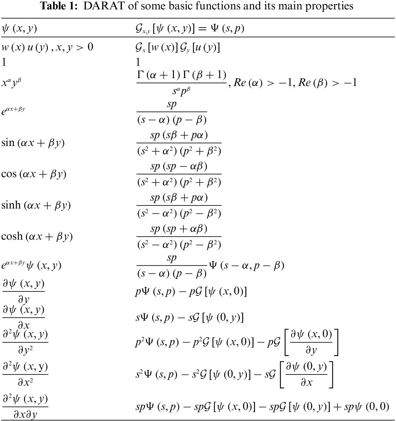
In the following, we present Table 1 to illustrate the values of the double ARA transform of some elementary functions and give main properties of the transform.
In this section, we introduce a new triple transform, called the triple ARA transform (TARAT), and derive some basic properties and establish certain results involving partial derivatives.
Definition 4.1. Let
where
Note that, the triple ARA transform is a linear transform, due to the fact that if
To simplify the application of the triple ARA transform, we need to recall the following notations:
By a similarity in the variables
The existence conditions of the triple ARA transform are presented in the following theorem.
Theorem 4.1. Let
where
Proof. Assume that
Also, the inverse triple ARA transform implies that
This finishes the proof of the theorem.
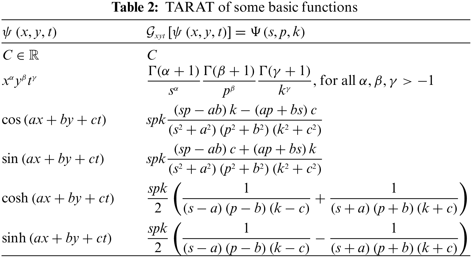
In Table 2, we provide some values of the triple ARA transform for some basic functions.
Now, we introduce some properties of the new approach.
Property 4.1. (Change of scale property) Let
where
Proof. Based on the definition of the triple ARA transform, we have
Putting
This finishes the proof of our result.
Property 4.2. (First shifting property) Let
where
Proof. Based on the definition of the triple ARA transform, we obtain
This finishes the proof of our result.
The following result is very useful in solving some kinds of partial differential equations.
Theorem 4.2. If
where
Proof: The definition of the triple ARA transform implies
From the properties of the single ARA, we get
Again, using some properties of the ARA transform to both variables
This finishes the proof of the theorem.
The application of triple ARA on partial derivatives of different types is illustrated on the following theorem.
Theorem 4.3. Let
i)
ii)
iii)
iv)
Proof (i). From the definition of the triple ARA transform, we write
To solve the integration inside the brackets, we use the idea of integration by parts with the assumptions that
(ii). By using part (i) of the theorem, it follows that:
where,
Similarly, one can follow the proof of (iii) and (iv).
This proves the theorem.
In view of the similarity between
The following property is a basic result from Theorem 4.3, and the proof can be obtained by similar arguments to the above theorem.
Corollary 4.1. Let
•
•
•
•
•
The following corollary presents a new application of the triple ARA transform, that is useful in solving some kinds of integral equations.
Corollary 4.2. If
Proof. Suppose that
and
Applying the triple ARA transform to both sides of Eq. (4), and using Theorem 4.3 suggest to write
Thus, we write
which implies that
This ends the proof of our corollary.
Now we study the effect of the triple ARA on the Heaviside function.
Theorem 4.4. Let
where
Proof. From the definition of the triple ARA transform, we have
Putting
Thus, we infer
This ends the proof of our theorem.
The following theorem presents the application of the triple ARA on the multi convolution property.
Theorem 4.5.(Convolution Theorem) If
where
Proof. Following the definition of the triple ARA transform, we write
The definition of the Heaviside function implies
Thus, we get
Using Theorem 4.4 reveals
This completes the proof of the theorem.
In this section, we present an algorithm for using the triple ARA transform in solving partial differential equations and provide solutions of some examples including partial differential equations.
5.1 Algorithm of the TARAT Method
To illustrate the method of using the triple ARA transform in solving partial differential equations, let us consider the following partial differential equation:
where
which yields
where
where
To obtain the solution in the original space, we apply the inverse triple ARA transform to Eq. (14) to have
Hence, the desired result is therefore established.
In this section, we apply the triple ARA transform operator to solve the wave equation, heat equation, Poisson equation and some few others.
Example 1: Consider the following wave equation
where
Solution: Operating the triple ARA transform to both sides of Eq. (5) yields
Hence, using the derivative properties implies
To simplify Eq. (17), we find the transformed values of the conditions (16) as follows:
By substituting the above values and using simple calculations, we can derive
Applying the inverse triple ARA transform
The following Fig. 1 illustrates the contours 3D plot of the exact solution to Example 1, with different values of the variables as follows.
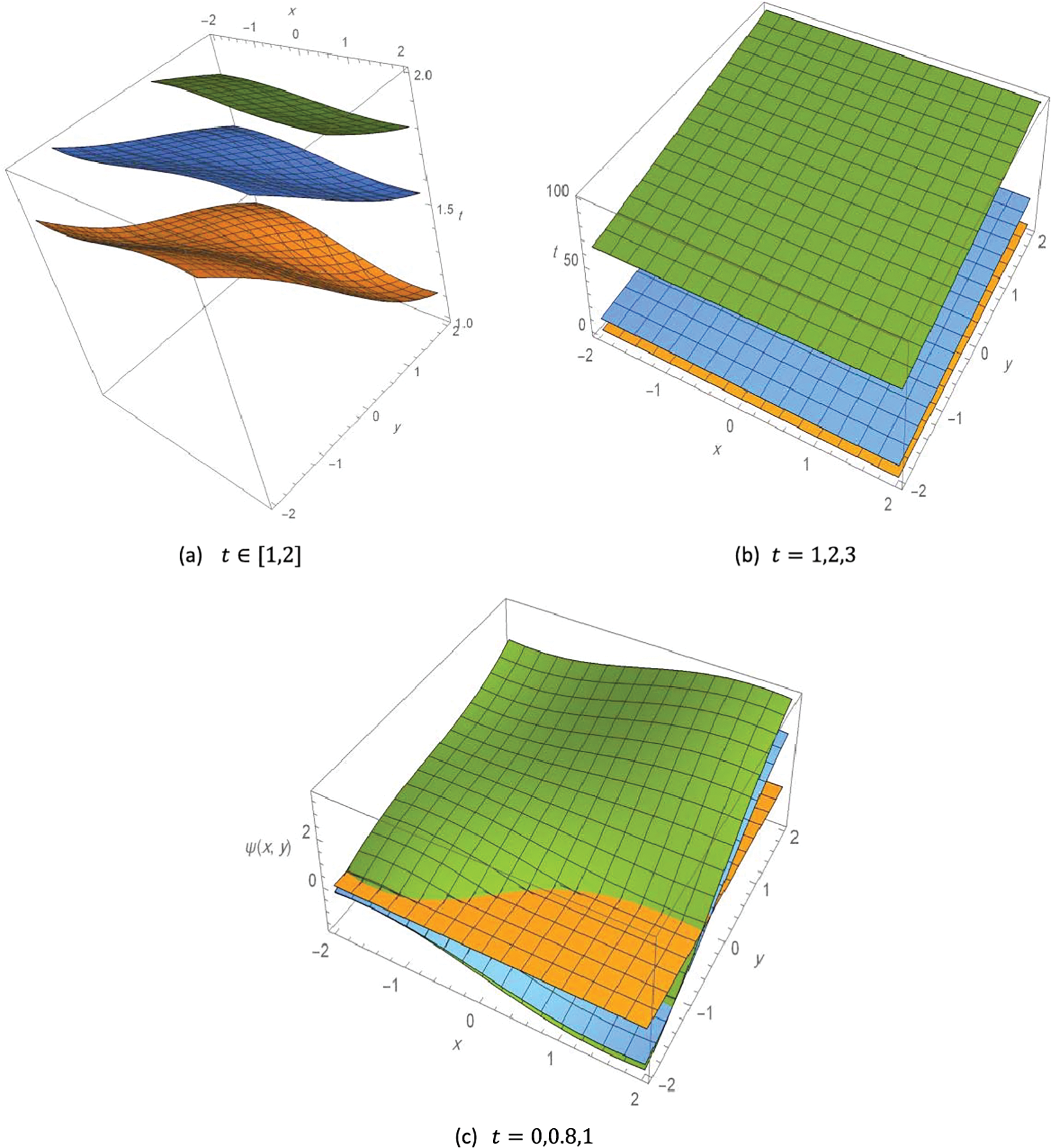
Figure 1: Contour 3D plot of the solution to Example 1,
Example 2: Consider the heat partial differential equation
where
Solution: Operating the triple ARA transform to both sides of Eq. (19) gives rise to
Employing properties of the derivative infer
To simplify Eq. (22), we compute the transformed values of the conditions as follows:
Substituting the above values included in Eq. (22) and applying some calculations we reach the conclusion
Applying the inverse
Our example has, therefore, been solved.
The following Fig. 2 illustrates the contours 3D plot of the exact solution to Example 2, with different values of the variables as follows.
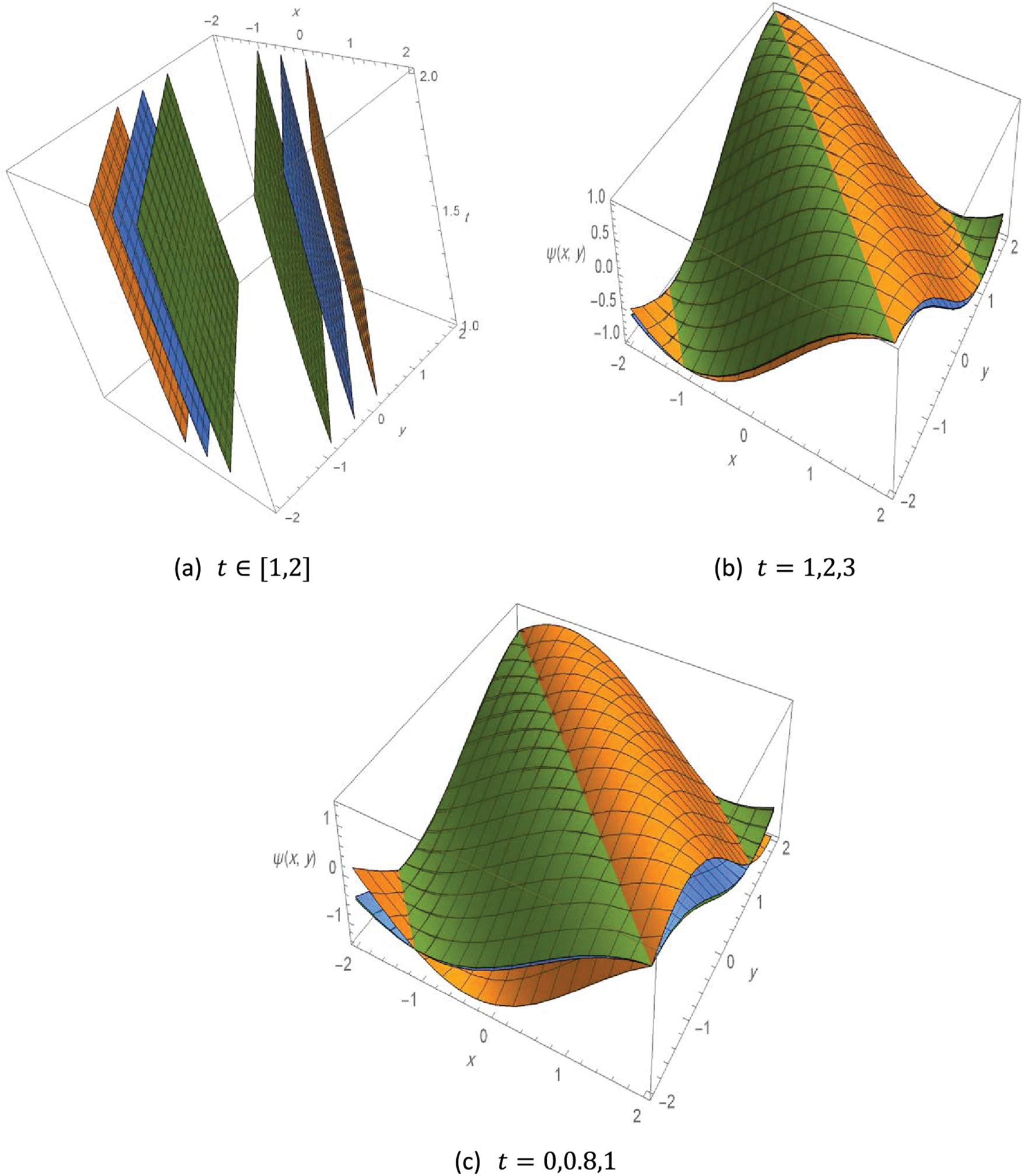
Figure 2: Contour the 3D plot of the solution to Example 2,
Example 3: Consider the following Poisson partial differential equation:
where
Solution: By arguments alike to those employed for Examples 1 and 2, we apply the TARAT to Eq. (24) and compute the transformed values of the initial conditions to infer
Thus, we have the solution, in the triple ARA space, as
Now, we reach the solution to Example 3 in the original space, by applying the inverse TARAT
Our example has been solved.
The following Fig. 3 illustrates the contours 3D plot of the exact solution to Example 3, with different values of the variables as follows.
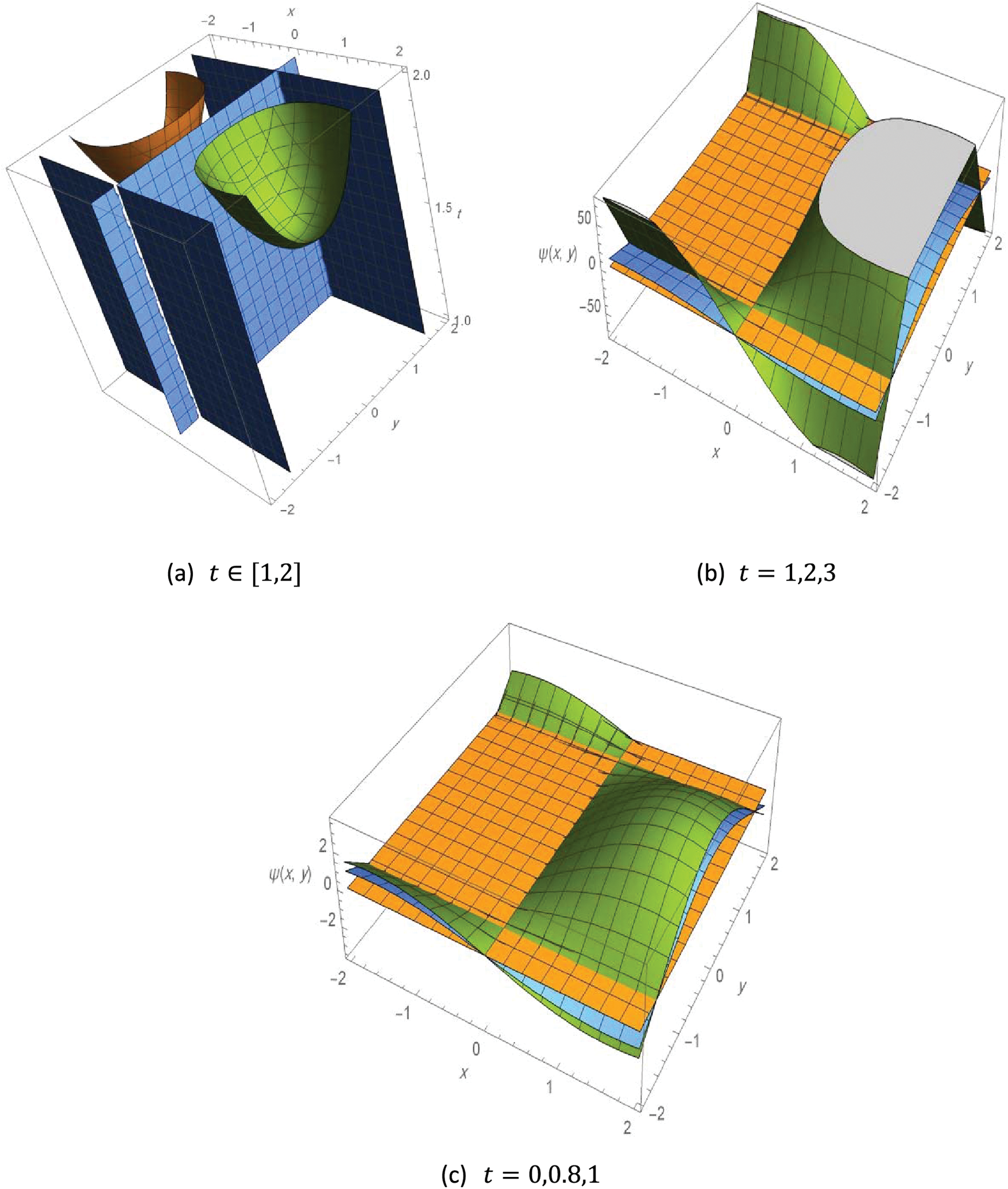
Figure 3: Contour 3D plot of the solution to Example 3,
Example 4: Consider the following Laplace partial differential equation:
where
Solution: Following steps alike to those used in the previous examples, then by applying the TARAT to the conditions in (28) and operating the triple ARA transform to Eq. (27) we establish that
Thus, we get the solution in the triple ARA space in the form
Following that, we get a solution to Example 4 in the original space after applying the inverse triple ARA transform
Our example has been solved.
The following Fig. 4 illustrates the contours 3D plot of the exact solution to Example 4, with different values of the variables as follows.
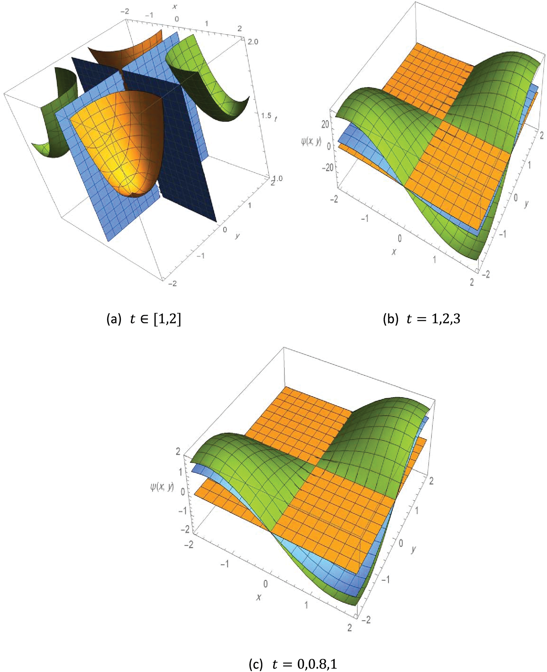
Figure 4: Contour 3D plot of the solution to Example 4,
Example 5: Consider the following partial differential equation
where
Solution: Applying the triple ARA transform to the condition (31) infers
Now, allowing the triple ARA transform to act on both sides of Eq. (31) and using the transformed values of the conditions with simple calculations reveal
This indeed implies
Operating the inverse TARAT
Our example has then been solved.
The following Fig. 5 illustrates the contours 3D plot of the exact solution to Example 5, with different values of the variables as follows.
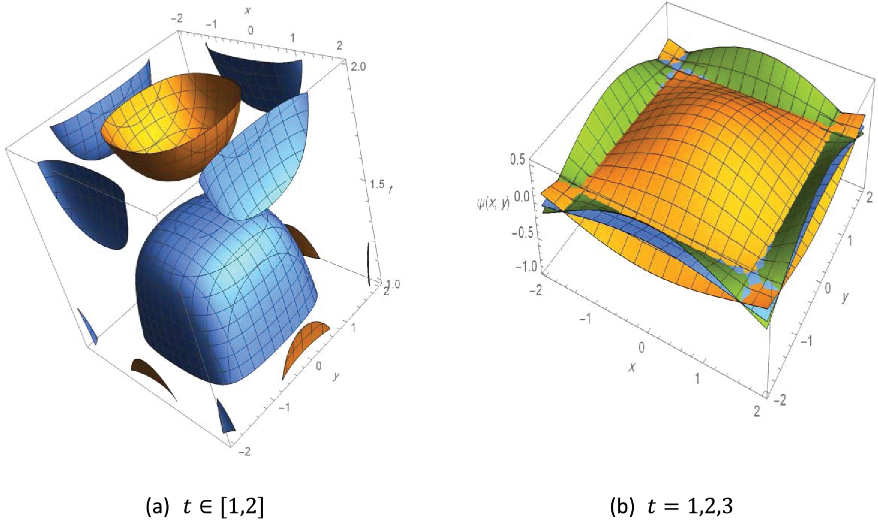
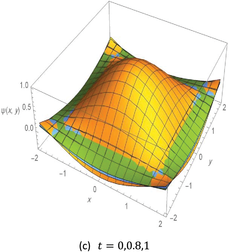
Figure 5: Contour 3D plot of the solution to Example 4,
In this paper, a new triple transform called the triple ARA transform is presented and several properties and theorems including linearity, existence, partial derivatives, and the multiple convolution theorem are introduced. Tables that summarize the new results are established to illustrate the new approach. The methodology of using the triple ARA transform in solving partial differential equations is given and further examples of several types of partial differential equations involving heat, wave, and Poisson equations are discussed. The outcomes have shown the simplicity of using the proposed transform in different aspects. In future work, we aim to solve integral equations and nonlinear partial differential equations based on the triple ARA transform.
Acknowledgement: Not applicable.
Funding Statement: This research received no external funding.
Author Contributions: All authors have read and agreed to the published version of the manuscript.
Availability of Data and Materials: Not applicable.
Conflicts of Interest: The authors declare that they have no conflicts of interest to report regarding the present study.
References
1. Ovsiannikov, L. V. E. (1982). Group analysis of differential equations. Academic Press. [Google Scholar]
2. Ovsiannikov, L. V. (1958). Groups and group-invariant solutions of partial differential equations. Doklady Akademii Nauk SSSR, 118(3), 439–442. [Google Scholar]
3. Bluman, G. W., Cole, J. D. (1969). The general similarity solution to the heat equation. Journal of Mathematics and Mechanics, 18(11), 1025–1042. [Google Scholar]
4. Saadeh, R., Alaroud, M., Al-Smadi, M., Ahmad, R. R., Salma Din, U. K. (2019). Application of fractional residual power series algorithm to solve Newell-Whitehead–Segel equation of fractional order. Symmetry, 11(12), 1431. [Google Scholar]
5. Saadeh, R. (2021). Numerical algorithm to solve a coupled system of fractional order using a novel reproducing kernel method. Alexandria Engineering Journal, 60(5), 4583–4591. [Google Scholar]
6. Saadeh, R., Al-Smadi, M., Gumah, G., Khalil, H., Khan, R. A. (2016). Numerical investigation for solving two-point fuzzy boundary value problems by reproducing kernel approach. Applied Mathematics and Information Sciences, 10(6), 2117–2129. [Google Scholar]
7. Saadeh, R., Burqan, A., El-Ajou, A. (2022). Reliable solutions to fractional Lane-Emden equations via Laplace transform and residual error function. Alexandria Engineering Journal, 61(12), 10551–10562. [Google Scholar]
8. Burqan, A., Saadeh, R., Qazza, A., Momani, S. (2023). ARA-residual power series method for solving partial fractional differential equations. Alexandria Engineering Journal, 62, 47–62. [Google Scholar]
9. Qazza, A., Burqan, A., Saadeh, R. (2022). Application of ARA-residual power series method in solving systems of fractional differential equations. Mathematical Problems in Engineering, 2022, 1–17. [Google Scholar]
10. Widder, V. (1941). The Laplace transform. Princeton, NJ, USA: Princeton University Press. [Google Scholar]
11. Atangana, A., Kiliçman, A. (2013). A novel integral operator transform and its application to some FODE and FPDE with some kind of singularities. Mathematical Problems in Engineering, 2013, 531984. [Google Scholar]
12. Al-Omari, S., Kilicman, A. (2013). An estimate of Sumudu transform for Boehmians. Advances in Difference Equations, 2013, 77. [Google Scholar]
13. Elzaki, T. M. (2011). The new integral transform “Elzaki transform”. Global Journal of Pure and Applied Mathematics, 7, 57–64. [Google Scholar]
14. Al-Omari, S. (2015). Natural transform in Boehmian spaces. Nonlinear Studies, 22(2), 291–297. [Google Scholar]
15. Saadeh, R., Qazza, A., Burqan, A. (2020). A new integral transform: ARA transform and its properties and applications. Symmetry, 12, 925. [Google Scholar]
16. Saadeh, R. Z., Ghazal, B. F. A. (2021). A new approach on transforms: Formable integral transform and its applications. Axioms, 10(4), 332. [Google Scholar]
17. Al-Omari, S. K., Kilicman, A. (2014). On the exponential Radon transform and its extension to certain functions spaces. Abstract and Applied Analysis, 2014, 612391. [Google Scholar]
18. Sedeeg, A. H. (2016). The new integral transform “Kamal Transform”. Advances in Theoretical and Applied Mathematics, 11, 451–458. [Google Scholar]
19. Al-Omari, S. K. (2016). On q-Analogues of the Mangontarum transform for certain q-Bessel functions and some application. Journal of King Saud University-Science, 28(4), 375–379. [Google Scholar]
20. Aghili, A., Parsa Moghaddam, B. (2011). Certain theorems on two dimensional Laplace transform and non-homogeneous parabolic partial differential equations. Surveys in Mathematics and its Applications, 6, 165–174. [Google Scholar]
21. Dhunde, R. R., Bhondge, N. M., Dhongle, P. R. (2013). Some remarks on the properties of double Laplace transforms. International Journal of Applied Physics and Mathematics, 3, 293–295. [Google Scholar]
22. Dhunde, R. R., Waghmare, G. L. (2017). Double Laplace transform method in mathematical physics. International Journal of Theoritical and Mathematical Physics, 7, 14–20. [Google Scholar]
23. Eltayeb, H., Kiliçman, A. A. (2013). A note on double Laplace transform and telegraphic equations. Abstract and Applied Analysis, 2013, 932578. [Google Scholar]
24. Alfaqeih, S., Misirli, E. (2020). On double Shehu transform and its properties with applications. International Journal of Analysis and Applications, 18, 381–395. [Google Scholar]
25. Sonawane, M., Kiwne, S. B. (2019). Double Kamal transforms: Properties and applications. Journal of Applied Science and Computation, 4, 1727–1739. [Google Scholar]
26. Ganie, J. A., Ahmad, A., Jain, R. (2018). Basic analogue of double Sumudu transform and its applicability in population dynamics. Asian Journal of Mathematics and Statistics, 11, 12–17. [Google Scholar]
27. Eltayeb, H., Kiliçman, A. (2010). On double Sumudu transform and double Laplace transform. Malaysian Journal of Mathematical Sciences, 4, 17–30. [Google Scholar]
28. Tchuenche, J. M., Mbare, N. S. (2007). An application of the double Sumudu transform. Applied Mathematical Sciences, 1, 31–39. [Google Scholar]
29. Al-Omari, S. K. Q. (2012). Generalized functions for double Sumudu transformation. International Journal of Algebra, 6, 139–146. [Google Scholar]
30. Eshag, M. O. (2017). On double Laplace transform and double Sumudu transform. American Journal of Engineering Research, 6, 312–317. [Google Scholar]
31. Ahmed, Z., Idrees, M. I., Belgacem, F. B. M., Perveenb, Z. (2020). On the convergence of double Sumudu transform. Journal of Nonlinear Science and Applications, 13, 154–162. [Google Scholar]
32. Idrees, M. I., Ahmed, Z., Awais, M., Perveen, Z. (2018). On the convergence of double Elzaki transform. International Journal of Advanced and Applied Sciences, 5, 19–24. [Google Scholar]
33. Ahmed, S., Elzaki, T., Elbadri, M., Mohamed, M. Z. (2021). Solution to partial differential equations by new double integral transform (Laplace-Sumudu transform). Ain Shams Engineering Journal, 12, 4045–4049. [Google Scholar]
34. Ahmed, S. A., Qazza, A., Saadeh, R. (2022). Exact solutions of nonlinear partial differential equations via the new double integral transform combined with iterative method. Axioms, 11(6), 247. [Google Scholar]
35. Ahmed, S. A., Qazza, A., Saadeh, R., Elzaki, T. (2022). Conformable double Laplace-Sumudu iterative method. Symmetry, 15, 78. [Google Scholar]
36. Saadeh, R., Qazza, A., Burqan, A. (2022). On the double ARA-Sumudu transform and its applications. Mathematics, 10, 2581. [Google Scholar]
37. Qazza, A., Burqan, A., Saadeh, R., Khalil, R. (2022). Applications on double ARA–Sumudu transform in solving fractional partial differential equations. Symmetry, 14, 1817. [Google Scholar]
38. Qazza, A., Burqan, A., Saadeh, R. (2021). A new attractive method in solving families of fractional differential equations by a new transform. Mathematics, 9(23), 3039. [Google Scholar]
39. Burqan, A., Saadeh, R., Qazza, A. (2021). A novel numerical approach in solving fractional neutral pantograph equations via the ARA integral transform. Symmetry, 14(1), 50. [Google Scholar]
40. Saadeh, R. (2022). Applications of double ARA integral transform. Computation, 10(12), 216. [Google Scholar]
41. Saadeh, R. (2022). Application of the ARA method in solving integro-differential equations in two dimensions. Computation, 11(1), 4. [Google Scholar]
42. Eltayeb, H., Bachar, I., Abdalla, Y. T. (2020). A note on time-fractional Navier-Stokes equation and multi-Laplace transform decomposition method. Advances in Difference Equations, 2020(1), 1–19. [Google Scholar]
43. Eltayeb, H., Bachar, I. (2020). A note on singular two-dimensional fractional coupled Burgers’ equation and triple Laplace Adomian decomposition method. Boundary Value Problems, 2020, 1–17. [Google Scholar]
44. Al-Omari, S. (2014). On the generalized Sumudu transform. Journal of Applied Functional Analysis, 9(1–2), 42–53. [Google Scholar]
45. Issa, A., Al-Omari, S., Naser, M., Al-Shawaqfeh, S. (2016). On Sumudu transforms and their applications to some initial value problems. Advances in Differential Equations and Control Processes, 17(4), 285–300. [Google Scholar]
46. Agarwal, P., Al-Omari, S. (2016). Some general properties of a fractional Sumudu transform in the class of Boehmians. Kuwait Journal of Science, 43(2), 206–220. [Google Scholar]
47. Al-Omari, S. K. (2018). On the quantum theory of the natural transform and some applications. Journal of Difference Equations and Applications, 25(1), 21–37. [Google Scholar]
Cite This Article
 Copyright © 2024 The Author(s). Published by Tech Science Press.
This work is licensed under a Creative Commons Attribution 4.0 International License , which permits unrestricted use, distribution, and reproduction in any medium, provided the original work is properly cited.
 Downloads
 Citation Tools