Multidomain Correlation-Based Multidimensional CSI Tensor Generation for Device-Free Wi-Fi Sensing

1  Introduction

With the widespread deployment of wireless infrastructure and the popularization of smart terminals, Wi-Fi WLANs have been widely deployed in our surroundings. Wi-Fi signals, which were previously solely used for data communication, can now provide pervasive sensing services thanks to the development and integration of technologies including wireless communication, the internet of things (IoT), and mobile computing [1–3].

The received signal strength indicator (RSSI) from the Wi-Fi MAC layer was usually used as the main sensing parameter previously. Due to the small-scale shadow fading caused by the indoor multipath effects (ME), the signal energy and the propagation path, however, are unable to maintain stable monotonicity, which results in the RSSI of multipath superposition failing to accurately reflect each path [4].

Since multipath propagation exhibits frequency selective fading, CSI as a frequency response parameter maintains a more stable data distribution than RSSI in a stable propagation space; meanwhile, it can exhibit noticeable differences when the spatial context changes in real-time [5]. Undoubtedly, using effective means to extract features reflecting different contexts from CSI is greatly beneficial to improve the performance of Wi-Fi sensing.

Compared with device-based active systems, the device-free passive Wi-Fi sensing technique has recently gained more attention because it is more suited for pervasive IoT applications [6,7]. However, in a complex room, the ME brings rich spatial information, meanwhile, it aggravates the non-stationary statistical characteristics of CSI. Although spatial variations are explicitly reflected in CSI measurements, subtle representational differences are typically masked by overall ME fluctuations, especially in the case of device-free sensing.

To overcome the above problems, most ML-based CSI sensing systems place hope on more complicated model structures, such as employing deep learning (DL) models, rather than trying to find answers in the CSI data itself, which restricts the performance upper bound of the built models.

As time, space, and frequency height correlation data, the CSI corresponding to the real-time scenario is an aggregate reflection of the parameter changes in these three domains. Some previous works have tried data preprocessing methods to smooth the feature learning of CSI [8–10]. In [8], the researchers used a 1-dimensional density clustering algorithm (i.e., CFDP) to classify the raw CSI, and then extract the inputs from the processed data to feed a deep neural network (DNN)-based model. Wang et al. [9] leveraged CSI phase difference for angle of arrival estimation, and then constructed a CSI image with 16-channel using the estimated values to improve model localization precision. However, due to the limitations of the algorithms themselves, these methods cannot fully exploit the temporal, spatial, and frequency information carried by CSI, resulting in the unsatisfactory overall performance of the sensing system.

In this paper, we propose a spatial-temporal-frequency correlation-based CSI tensor generation method, aiming to provide a better input scheme for ML-based sensing systems. First, we use real-world CSI measurements to quantitatively verify the time-frequency correlation of the CSI magnitude. Based on this characteristic, we formulate a time-frequency correlated CSI amplitude matrix and confirm its low-rank property. Second, combined with MIMO spatial diversity, we extend the CSI magnitude matrix into a 3-order CSI tensor associated with temporal, spatial, and frequency information. Third, a novel matrix factorization algorithm is proposed to separate the structured information and context fluctuations in the CSI; meanwhile, the CSI gradients w.r.t time and frequency changes are calculated. Finally, we generate the multidimensional tensor by combining the matrix factorization result with two gradient matrices, which can be used to feed an ML-based CSI sensing model.

The rest of the paper is organized as follows. Section 2 reviews the related work on CSI sensing. In Section 3, we introduce some preliminaries. Section 4 introduces the proposed method in detail. The experimental evaluation is conducted in Section 5. The conclusion is drawn in Section 6.

2  Related Work

For the research of device-free Wi-Fi sensing, Youssef et al. [6] first proposed a fingerprint-based method, in which the RSSI fingerprints of the target at different locations were first constructed, and then the target location was estimated via comparing the online data with the fingerprints; Zhang et al. [11] proposed a model-based solution and used geometric methods to calculate the target position. Since 2010, following the pioneering work of Halperin et al. [5], the CSI has gradually become the leading role in the field due to its refined metrics, and research on device-free localization using CSI has been emerging.

Xiao et al. [12] proposed a passive localization system Pilot exploiting CSI frequency diversity, which used an anomaly detection module to determine the target, the location was then estimated by fingerprint matching. Experimental results showed that the Pilot significantly outperformed RSSI-based methods. In [13], researchers built a single TX/RX pair system MonoStream. MonoStream created CSI at different locations as image data and extracted discriminative contextual features, and achieved location inference with an accuracy of 0.95 m through multiple binary classifiers. From the perspective of geometric relationship, Qian et al. [14,15] established the Widar system between the target position and CSI variation and achieved a decimeter-level tracking error of about 30 cm.

Recently, due to the powerful nonlinear description capability of DL, researchers have also applied this cutting-edge technique to CSI device-free localization and have spawned many promising solutions [10,16]. Gao et al. [17] proposed a device-free localization system DFLAR based on a radio image processing. DFLAR used the amplitude and phase of CSI to generate radio images, and then extracted color and texture features using algorithms such as Gabor filters. The deep auto-encoder network as a classifier finally performed the mapping of features to object locations. Zhou et al. extracted the most contributing feature information in CSI using density-based clustering algorithm and principal component analysis (PCA), In their two studies, support vector machine (SVM) [18] and deep BP networks [19] were employed to conduct the regression of CSI feature vector to location, respectively. Li et al. [8] used the DNN embedded with the domain adaptation mechanism as the localization model, by which they realized the transformation of the concatenating vector of CSI amplitude and phase to spatial coordinates. In [20], the researchers applied the phase calibration method to improve the CSI phase shift caused by synchronization issues, and used an enhancement measure based on the structural similarity to expand the manually collected samples, achieving an efficient an efficient and lightweight model.

In two recent studies involving CNN, COMUTE [21] represented multi-link CSI time-frequency information as multi-channel input images, and realized device-free localization based on the CNN using multi-label classification framework. In [3], the authors created a 2D array based on the CSI magnitude difference, and utilized two deep CNNs to learn two plain coordinate features of the target location, and performed coordinates quantization through two cascaded SVMs and regression functions.

However, most existing ML-based CSI sensing solutions usually suffer from the following two problems: (1) The created input does not fully utilize the spatial and time-frequency information carried by CSI, resulting in a lack of sufficient resolution for spatial context changes. (2) The constructed model focuses on the precise mapping of CSI to sensing targets, but ignores subtle data fluctuations caused by small contextual changes. These problems frequently make most sensing solutions struggle with sufficiently reliable performance, resulting in an unsmooth research process. To eliminate the above-mentioned barriers as much as possible, we carried out this work.

3  Preliminaries

3.1 Channel State Information

The CSI is the sampling of the subchannel (subcarrier) frequency response of the Wi-Fi link, and it can be resolved using the IEEE 802.11n wireless network interface cards (NIC) with modified firmware. There are currently two open-source tools available for modifying firmware in the Linux operating system, the 802.11n-CSI Tool [22] for Intel 5300 NIC and the Atheros CSI [23] for Atheors 9k series NICs.

Atheros CSI can resolve 56 (or 114) subcarriers under 20 MHz (or 40 MHz) Wi-Fi bandwidth but requires two computers with Atheors NICs. For deployment convenience, our experimental scenario is configured with a 3-antenna AP and a computer 5300 NIC. In 2.4G/20 MHz mode, each MIMO-OFDM spatial stream (TX/RX antenna pair) can resolve 30 subcarriers, and thus the CSI in each valid packet can be expressed as:

C=[h1,1⋯h1,3h2,1⋱h2,3h3,1⋯h3,3]=[ht,r]∈C3×3×K(1)

where ht,r=[hf1,hf2,…,hfK] denotes the CSI vector of spatial stream t-r, and K = 30. hfk=|hfk|ej/_hfk is the CSI at subcarrier k with center frequency fk, |hfk| and /_hfk represent the amplitude-frequency and phase-frequency response, respectively.

Due to the influence of environmental interference, protocol specifications, etc., the obtained raw CSI contains a significant amount of abrupt noise and outliers. Therefore, in order to ensure the validity and reliability of the data and minimize the impact of additional factors on system performance, it is necessary to preprocess the raw measurements. Preprocessing means often include outlier removal, data interpolation, noise filtering. Since the related methods have been described and applied in numerous publications [24–26], this procedure will not be covered in detail here.

3.2 CSI Amplitude Characteristics

Fig. 1 shows the distribution of CSI amplitudes for 30 s in four random spatial contexts (namely, the sensing target at four random locations). It can be seen that for any spatial stream, the amplitude of subcarriers shows consistency along the time axis; meanwhile, different subcarriers have similar amplitude variation trends.

Figure 1: CSI profiles in different spatial contexts. (a) CSI measurements from 1–1 spatial stream, target at random location 1. (b) CSI measurements from 1–1 spatial stream, random location 2. (c) 2–3 spatial stream, location 2. (d) 3–2 spatial stream, location 2

Such phenomenon intuitively suggests the time-frequency correlation of the amplitude vector |ht,r|, which is the cornerstone for the low-rank property of the CSI. In the following section, we perform singular value decomposition (SVD) of CSI matrices from different spatial contexts, demonstrating this property quantitatively.

4  Proposed Method

In this section, we detail the proposed method, including formulation of amplitude-based CSI matrix and its low-rank property validation, distributed low-rank factorization algorithm, and multi-dimensional CSI tensor generation.

4.1 CSI Matrix

Numerous previous studies have shown that the CSI amplitude parameter is more stable than its phase, and thus we formulate the CSI matrix based on the amplitude.

First, the amplitude of the vector ht,r in preprocessed C is calculated, and get a spatial stream amplitude vector of k-dimensional, as follows:

h¯=(h∘h∗)t,r=[|hf1|,|hf2|,…|hfk|,…,|hfK|](2)

where ‘◦’ represents the Hadamard product.

And then, N amplitude vectors h¯ form a CSI matrix in temporal order, expressed as:

Hi=[h¯1;h¯2;...;h¯N]=[h¯1,1h¯1,2⋯h¯1,Kh¯2,1h¯2,2⋯h¯2,K⋮⋮⋱⋮h¯N,1h¯N,2⋯h¯N,K]=[h¯n,k]∈RN×K(3)

Compare Eq. (2), here h¯n,k=|hfk|. The CSI matrices adjacent to Hi in the same spatial stream are expressed as:

Hi±1=[h¯1±ΔN;h¯2±ΔN;...;h¯N±ΔN](4)

In the experimental environment of this paper, to take into account the real-time and packet-loss rate, the RX ping rate is set to 100 packets/s. Considering the information coverage of matrix and the target moving speed in the real case, the length of Hi along the time axis is set to be 0.5 s, and hence N = 50; meanwhile, the time span of adjacent CSI matrices is set to 0.1 s, namely, the sliding step of h¯ is ΔN = 10. The generation of any Hi can be illustrated as in Fig. 2.

Figure 2: CSI matrices generation illustration

Based on the formulated CSI matrices, we perform SVD of CSI matrices from different spatial contexts, demonstrating this property quantitatively. The results are shown in Fig. 3.

Figure 3: Singular values proportion of the CSI matrices. The total number of matrices is 6,000

In the decomposition results of Fig. 3, the first few singular values (SVs) of Hi share most energy of the matrix, while the SVs generated by context fluctuations account for a small proportion. Fig. 3 visualizes the potential low rank of Hi, and next we propose the distributed matrix factorization algorithm based on this property. For simplicity, the following parts replace Hi with H.

4.2 Distributed Low-Rank Matrix Factorization

For a matrix H with low rank (or approximately low rank), it can be decomposed into H = I + F, where I denotes a strong low-rank matrix, and F is fluctuating data. In real cases, I is the stable structured channel information, and F corresponds to the fluctuations caused by various types of communication interference. In theory, solving I and F can be achieved by minimizing the rank of I, expressed as:

minIrank(I)s.t. I+F=H;I,F,H∈RN×K(5)

Problem (5) is a typical NP-hard problem [27], which can be transformed into

minI,F‖I‖∗+λ‖F‖2,1s.t. I+F=H;I,F,H∈RN×K(6)

where ‖F‖2,1=∑k=1K∑n=1N([F]n,k)2 aims to sparse the column vectors. ‖‖∗ represents the nuclear norm and ‖‖∗ is ℓ2,1 norm, λ is a ratio adjustment hyperparameter with the purpose of following the scenario fluctuation strength.

The main method to solve problem (6) is a numerical iterative algorithm [28–30], and given the accuracy requirements of the localization as well as the norm convexity, this paper proposes a distributed matrix factorization algorithm (DMFA) based on the alternating direction method of multipliers (ADMM) [31]. First, problem (6) is formulated as a Lagrangian function:

ℒ(I,F,V,ρ)=‖I‖∗+λ‖F‖2,1−⟨V,H−I−F⟩F+ρ2‖H−I−F‖F2(7)

where ⟨⋅,⋅⟩F and ‖‖F denote the Frobenius inner product and norm, ρ is a penalty factor and V is a multiplier matrix.

Second, the Frobenius operations in Eq. (7) is transformed as follows:

−{⟨V,H−I−F⟩F−ρ2||H−I−F||F2}=−tr{(H−I−F)TV−ρ2(H−I−F)T(H−I−F)}=ρ2||H−I−F−1ρV||F2−12ρ||V||F2(8)

Therefore,

ℒ(I,F,V,ρ)=||I||∗+λ||F||2,1+ρ2||H−I−F−1ρV||F2−12ρ||V||F2(9)

Finally, the parameters in problem (9) are solved in a distributed manner based on the ADMM framework, as follows:

•   Fix the remaining and update F.

ℒ(F)=λ||F||2,1+ρ2||Δ−F||F2=λ∑k=1K(∑n=1N[F]n,k2)12+ρ2∑k=1K∑n=1N[Δ−F]n,k2≤λ∑k=1K∑n=1N[|F|]n,k+ρ2∑k=1K∑n=1N[[Δ]n,k−[F]n,k]2=defΦ(F)(10)

Let ∀fn,k∈{[F]n,k},∀δn,k∈{[Δ]n,k}, and define a function:

ϕ(fn,k)=λ|fn,k|+ρ2(δn,k−fn,k)2(11)

Apparently, here is Φ(F)=∑k=1K∑n=1Nϕ(fn,k). Introduce the Sign function and calculate partial derivative ∇fϕ(fn,k)=λsgn(fn,k)+ρ(fn,k−δn,k), and then the minimum can be given by:

arg⁡minfn,kϕ(fn,k)={δn,k+λ/ρδn,k≥λ/ρ0|δn,k|<λ/ρδn,k+λ/ρδn,k≤−λ/ρ(12)

Introduce a shrinkage operator 𝒮τ(x)=defsgn(x)⋅max(|x|−τ,0) and the Eq. (13) is expressed as:

arg⁡minfn,kϕ(fn,k)=𝒮λ/ρ(δn,k)(13)

Then, the optimal F∗ can be given by:

F∗=∑fn,karg⁡minfn,kϕ(fn,k)=𝒮λ/ρ(Δ)(14)

Ultimately, updated Fj can be expressed as:

Fj:=𝒮λ/ρ(H−Ij−1−1/ρVj−1)(15)

•   Fix other parameters and update I.

According to Eq. (9), there are:

ℒ(I)=||I||∗+ρ2||H−I−F−1ρV||F2(16)

And the optimal I∗ can be given by:

I∗=arg⁡minI||I||∗+ρ2||H−I−F−1ρV||F2=arg⁡minI1ρ||I||∗+12||I−(H−F−1ρV)||F2(17)

Introduce the singular value threshold function [16]:

𝒟τ(X)=defU𝒮τ(Σ)WT,𝒮τ(Σ)={σi−τ0σi>τ0≤σi≤τ(18)

where U and W are the left and right orthogonal matrices, and Σ denotes the singular values diagonal matrix. Thus, update I is expressed as:

Ij:=𝒟1/ρ(H−Fj−1/ρVj−1)(19)

• Fix other parameters and update V.

ℒ(V)=ρ2||H−I−F−1ρV||F2−12ρ||V||F2(20)

Eq. (20) is strongly convex, and hence its minimum can be obtained by partial derivative:

∇Vℒ(V)=∂∂Vtr{ρ2(H−I−F−1ρV)T(H−I−F−1ρV)−12ρVTV}=−(H−I−F)(21)

Update V can be expressed as:

Vj:=Vj−1−ρ(H−Ij−Fj)(22)

•   Introduce amplification factor α>1 and update ρ.

ρj:=min(ρmax,αρj−1)(23)

The DMFA implementation is outlined in Table 1. The finally obtained structured matrix I and fluctuation matrix F will be used as the main part of the input to drive the model input.

The proposed DMFA can distribute the coupled objective into multiple simple sub-optimizations, and uses the alternate parameters update to reach the optimal value, which ensures the stability of the global optimization. Compared with some commonly used means, such as Gabor filter [17], PCA [24], and Wavelet [32], a significant advantage of DMFA is the ability to adapt to the CSI fluctuations incurred by different contexts.

4.3 CSI Time-Frequency Gradient

To further characterize the CSI differences in different spatial contexts, the variation information of the CSI matrix along the time and frequency axes is calculated.

The gradient matrix of CSI w.r.t temporal variation is expressed as:

∇nH=[h¯2−h¯1;h¯3−h¯2;…;h¯N−h¯N−1]=[h¯2,1−h¯1,1⋯h¯2,K−h¯1,K⋮⋱⋮h¯N,1−h¯N−1,1⋯h¯N,K−h¯N−1,K]=[h¯n′,k]∈R(N−1)×K(24)

The gradient matrix of CSI w.r.t frequency diversity is:

∇kH=[h¯1,2−h¯1,1⋯h¯1,K−h¯1,K−1h¯2,2−h¯2,1⋯h¯2,K−h¯2,K−1⋮⋱⋮h¯N,2−h¯N,1⋯h¯N,K−h¯N,K−1]=[h¯n,k′]∈RN×(K−1)(25)

Moreover, to make the gradient matrices and CSI matrix consistent in size to facilitate the generation of final input, we extend them with the all-zero vector, as follows:

∇nH=[∇nH;[0]1×K]∈RN×K∇kH=[∇kH,[0]N×1]∈RN×K(26)

4.4 Multidimensional CSI Tensor

According to the same time node, we first concatenate the H of 3 × 3 MIMO spatial streams into a 3-order tensor, as follows:

H=[[H(0)],[H(1)],…,[H(8)]]∈R9×N×K(27)

Ultimately, the structured matrix I, the fluctuation matrix F, and two gradient matrices together constitute the CSI multidimensional input data, which is used to drive a sensing model. Referring to Eq. (27), the generation approach is expressed as:

X=[[[I(0)],[I(1)],…,[I(8)]],[[F(0∼8)]],[[∇nH(0∼8)]],[[∇kH(0∼8)]]]4×N×K×9(28)

Our X contains spatial and time-frequency information, which can describe the spatial context from multiple dimensions; meanwhile, the introduced gradient matrices are beneficial for the sensing model to capture small target changes. These advantages can effectively enhance the fine-grainedness and richness of input data, thereby effectively enhancing the accuracy and stability of ML-based models representation learning.

5  Experimental Study

In this section, we evaluate the proposed method with CSI data from typical indoor scenarios. We take device-free localization as the main case, and the input generation methods used by several state-of-the-art systems are chosen as the benchmarks, namely, CSIi [3], CiFi [9], and DFLAR [17]. The CNN-SVM [3] and 3D CNN-GRU model (see Fig. 4) we built are employed to perform location inference.

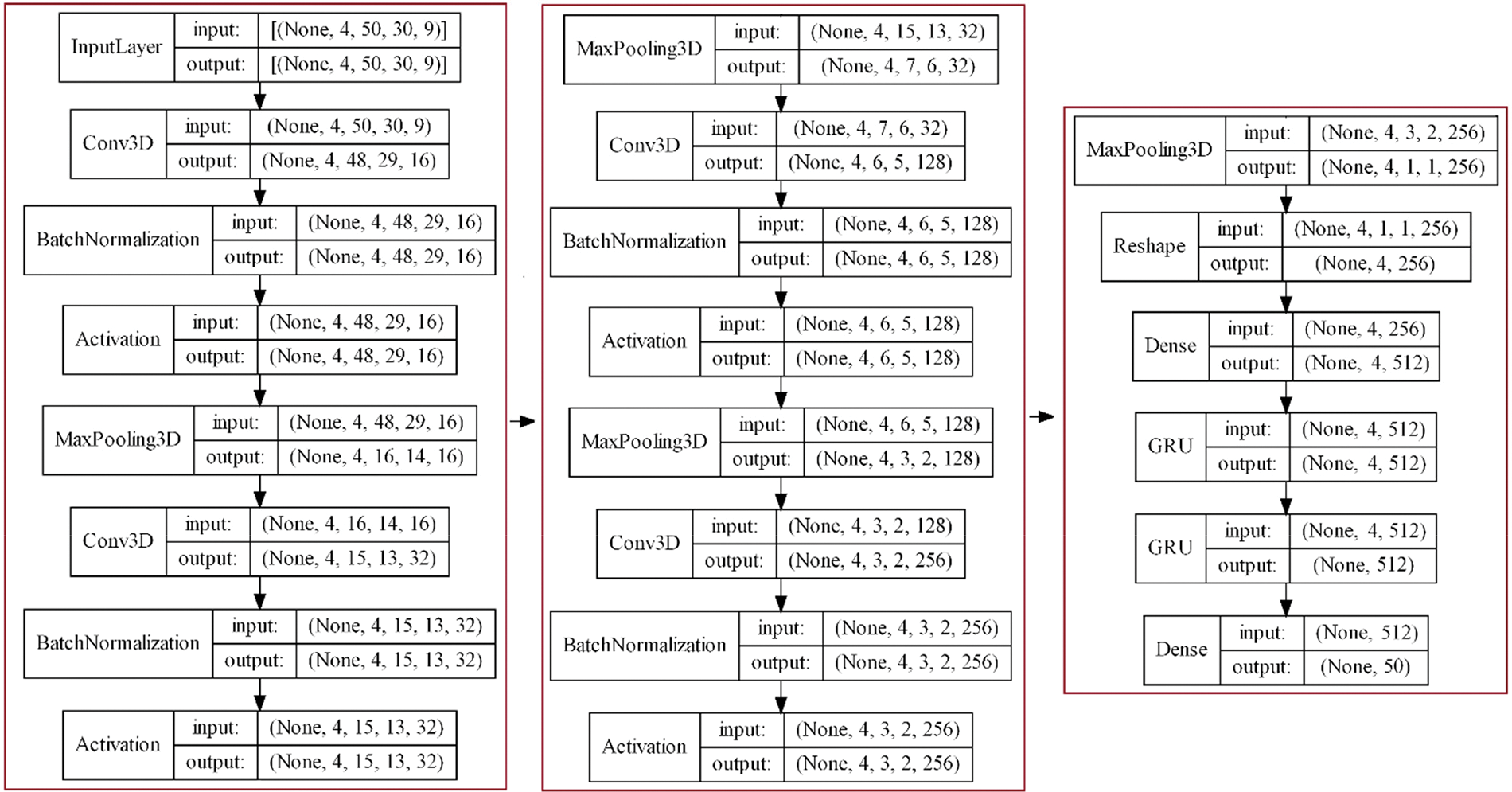
Figure 4: Illustration of 3D CNN-GRU model (by the “plot_model” of TensorFlow)

5.1 Experiment Configuration

The experimental scenario is shown in Fig. 5. The TX adopts a TL-WR882n wireless router with 3 antennas, the working mode is 2.4 GHz/20 MHz. The RX is a PC with Intel 5300 NIC, and the system is Ubuntu 12.04 LTS, the packet Ping rate is 100/s. The proposed algorithm DMDA is implemented with CVXPY 1.2, and the test models are built based on TensorFlow 2.6.0 and GeForce RTX 3070 Ti.

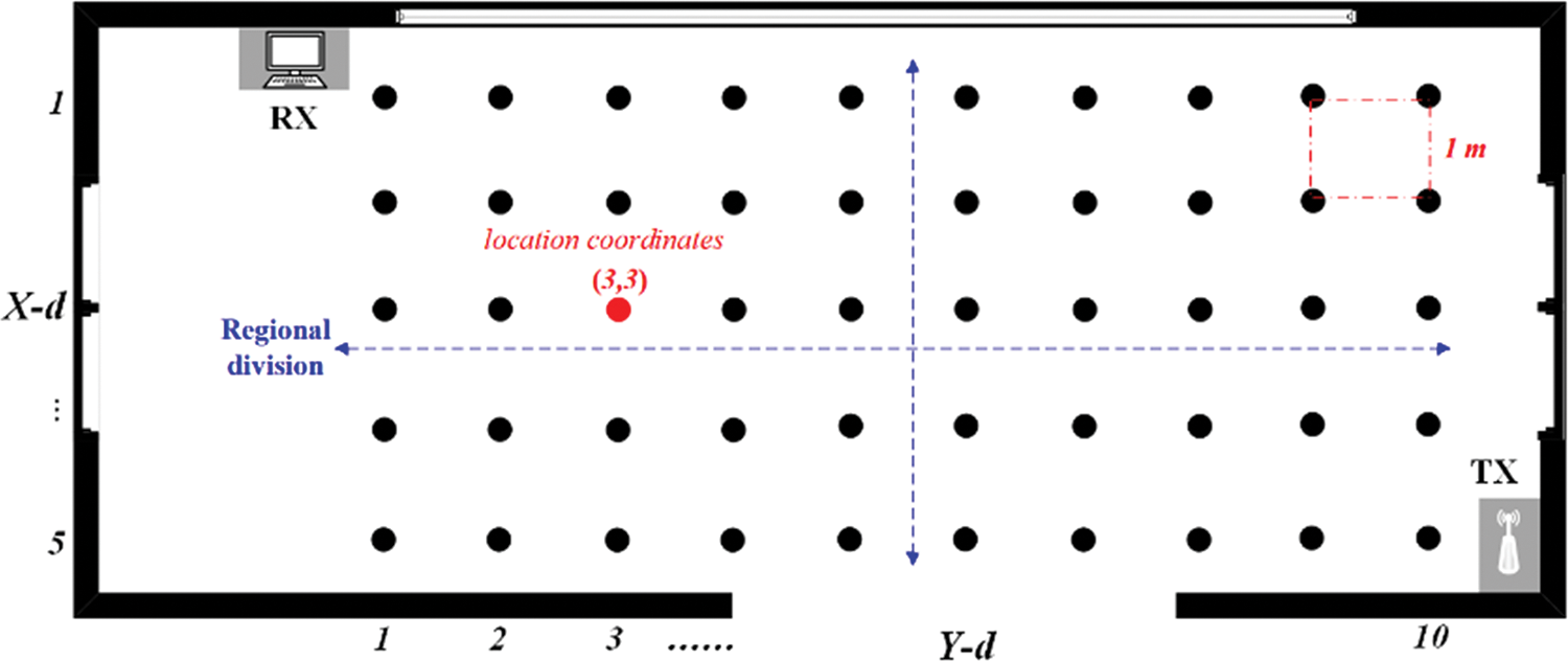
Figure 5: Layout of indoor experiment scenario

The database come from field-collected CSI, and a total of 5 targets (volunteers) participate. They performed single-target CSI acquisition at 5 different periods, traversing each reference point (RP) in the scenarios. The data of 3 targets were used for model training and testing, and we collected 3 min of data per period at each RP, resulting in a total of 270,000 CSI measurements, that is, 3 min × 60 s × 100 packets/s × 5 periods × 3 volunteers. Combining Section 4.1 and Fig. 2, the number of available CSI matrices is:

270,00−N+ΔNΔN=270,00−50+1010=26,996(29)

Removing invalid data, each RP finally has 20,000 training samples and 5,000 testing samples, called TS-I.

The other 2 acted as unknown targets, and 5,000 test samples were generated at each RP. Their data was solely used for testing the trained model, called TS-II.

5.2 Overall Evaluation

Since our method utilizes a classification pattern, we adopt the discretization evaluation instead of the absolute location error, in which the accuracy rate of inferring target locations is used as the criterion.

Based on the 3D CNN-GRU model trained by TS-I, we randomly select 30 RPs for testing. Each RP is evaluated 5 rounds with 500 random samples per round, and the result takes the average accuracy of 30 RPs. The overall performance is shown in Fig. 6.

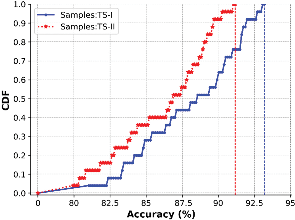
Figure 6: Overall test results of the proposed method

From the obtained accuracy rate CDF, it can be seen that the proposal achieves good inference results. The average accuracy of TS-I reaches more than 90%, of which more than half of the tests are above 88%. In the test of unknown targets, due to the individual differences of the targets, the inference ability has declined, with an average accuracy rate of slightly less than 89%, however, more than 60% of the tests are still above 85%.

The main reason is that the generated multidimensional CSI input more thoroughly incorporates the spatial and time-frequency data, which enables the localization model built using the data-driven paradigm to have a richer and more fine-grained feature base, and guarantees the data requirements of accurate mapping between CSI and RPs from the source. In addition, the employed 3D CNN-GRU can mine more differentiated features from three dimensions, improving the correct matching rate of features and RPs, which is also a positive contribution to better accuracy.

Considering the real-time requirements of some sensing tasks, we analyze the computational complexity of DMFA and the entire system in terms of elapsed time, based on the 3D CNN-GRU. The core hardware used in the test are Intel i5-11400 CPU and 16 GB RAM. Table 2 shows the running time of DMFA and the entire system. Due to the relatively small scale of the generated CSI input, the computational cost of the models is negligible with the current devices, and thus the time overhead of execution is mainly derived from the CSI data processing, that is, the execution of DMFA.

It can be seen that the DMFA accounts for about 83.2% of total overhead, in which computing matrix I takes over 82% of the time. Combined with the actual activity situation of indoor targets and the generation method of CSI matrix, the overall execution time is tolerable.

5.3 CSI Tensor Ablation Study

This part evaluates the benefits of the generated CSI tensor based on the 3D CNN-GRU, and the contribution of each component in the tensor by means of comparison.

We separately test the effect of 4 data modes (refer to Eq. (28)), including that the input is H or I only, or I + F, or CSI tensor. The samples are from TS-I and the RPs number is 25, and the test scheme is the same as Fig. 6. The results are shown in Fig. 7.

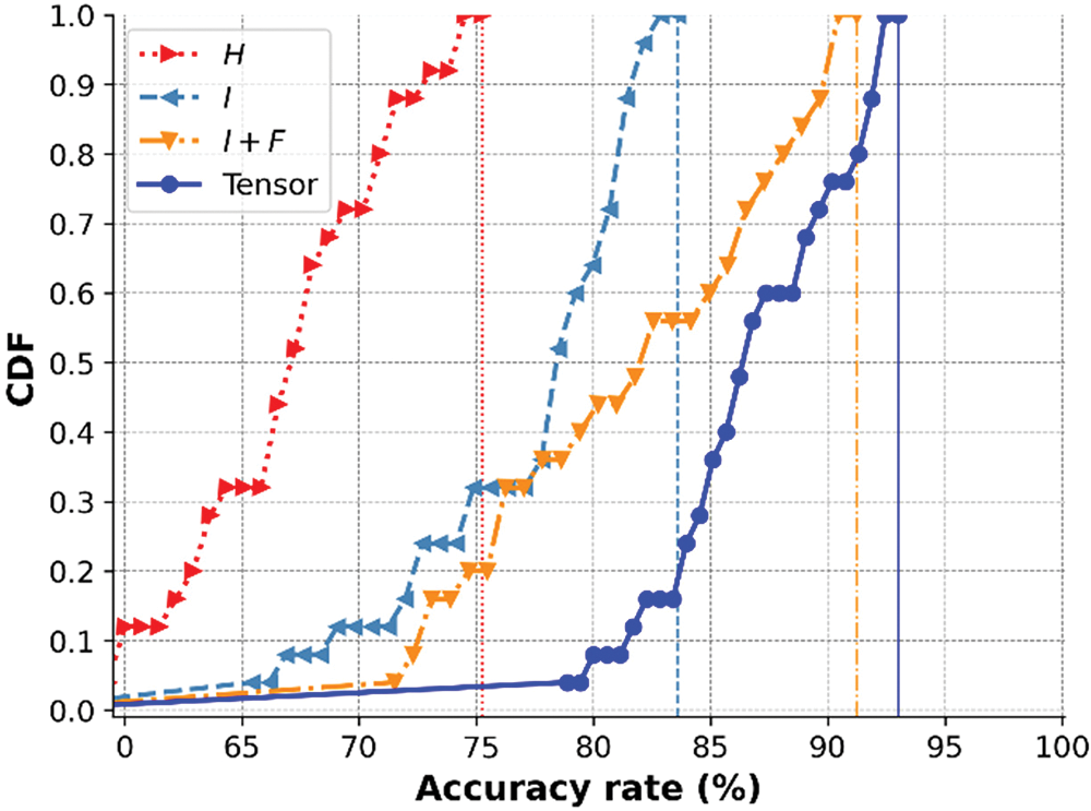
Figure 7: Contribution comparison of different components in CSI tensor

First, due to the richness and fine-grainedness of the generated CSI input, the CSI tensor provides clear advantages over adopting the raw CSI matrix H, with an average accuracy gain of roughly 20%.

Second, the I produced by the proposed DMFA makes a bigger contribution to the right inference. Compared to the other three CDFs, using the structured data I alone can achieve about 10% performance improvement, which also demonstrates the stability of the parameter CSI from the physical link layer.

Third, adding contextual fluctuation information, namely, I + F, greatly improves the performance upper limit of the sensing model, and the accuracy of half of the tests increases from less than 80% to about 85%.

Finally, adding the time and frequency variation of CSI, namely, ∇nH and ∇kH, is of great help to the inference stability. Compared with the CDF of ‘I + F’, the proportion of tests with lower accuracy dropped from over 1/2 to 1/3. The reason is that the gradient information greatly weakens the co-domain noise through differential calculation, thereby improving the resolution of CSI characterization.

5.4 Quantitative Evaluation

To further quantify the error distribution, we randomly selected 4 representative RPs for testing, that is, the region boundary RP L1 with location coordinates (LC) (X_d = 3, Y_d = 5), the edge RP L2 with LC (1, 10), two region central RPs L3 (5, 7) and L4 (2, 3). 100 random samples from TS-I are selected for each RP, and the criterion is the LC deviation (LCD), which is expressed as:

ei=|X−di−X−di,j¯|+|Y−di−Y−di,j¯|(30)

where [X−di,Y−di] denotes the actual RP location, and [X−di,j¯,Y−di,j¯] represents the inferred result with sample j. The test results are shown in Fig. 8.

Figure 8: Quantified LCD distribution

The test finds still suggest that the error of edge L2 is significantly lower than the others, with only 2 incorrect judgements and an LCD absolute value that does not surpass 2. The region boundary L3 has the highest error rate of 14%, but most LCD absolute values are below 3 and only one exceed 4. Although the LCD test performed is a single case study, it more intuitively supports the conclusions of the aforementioned overall performance test, and quantifies the benefits of the proposed method on system performance.

5.5 Comparison and Analysis

To highlight the advantages of the proposed DMFA, we compare it with three commonly used CSI preprocessing algorithms, namely, Gabor filter [17], PCA [24], and Wavelet [32], employing the 3D CNN-GRU as the execution model.

Given the data processing mechanism of the three comparison algorithms, we need to regularize the shape of the data they feed to the 3D CNN. For the PCA, we follow reference [24] but take all 30 principal components, and the Gabor and Wavelet process the raw 1 × 30 measurements directly. Next, we formulate them into an array of 50 × 30 × 9 (nine spatial streams) according to Fig. 2, and then concatenate four identical arrays into a tensor of 4 × 50 × 30 × 9. The test scheme is the same as Fig. 6, and the comparison results are shown in Fig. 9.

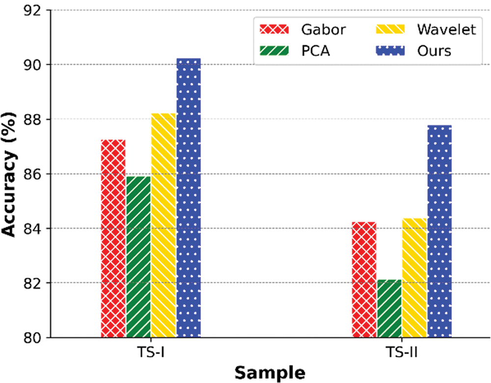
Figure 9: Average accuracy of four preprocessing algorithms

From the comparison results, it can see that our strategy produces the best outcomes based on the same deep model. In the test using TS-I samples, the average accuracy exceed 90%; while for the unknown targets, an average accuracy is about 87.8%. The PCA performs the worst, with an accuracy of only 85.92% and 82.14% in the two cases, respectively. The reason is that the PCA extracts features by eliminating the correlation of the data and assumes that this correlation is linear. Therefore, for the CSI with strong nonlinear dependencies, an ideal result is difficult to achieve.

Further, to demonstrate the overall superiority of the proposed method, we compare it to three state-of-the-art systems, namely, CSIi [3], CiFi [9], DFLAR [17], based on the 3D CNN-GRU.

We randomly select 25 RPs for testing. Each RP is evaluated 5 rounds with 500 random samples, and the result takes the average accuracy of 30 RPs. The comparison results based on 3D CNN-GRU are shown in Table 3.

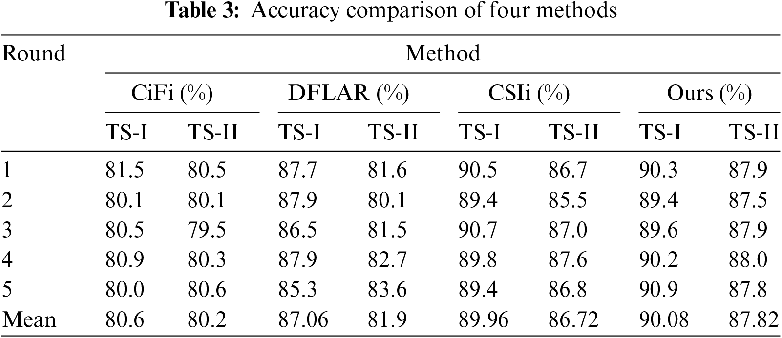
From the obtained accuracy, it can be seen that ours achieves good inference results. The average accuracy of TS-I reaches more than 92%; in the test of unknown targets, due to the individual differences of the targets, the inference ability has declined, with an average accuracy of slightly less than 90%.

The CiFi only utilizes the single and original two-dimensional CSI, and does not make use of the rich CSI information, resulting in it fail to identify potential differences well and thus the worst results. The DFLAR adds the two-dimensional phase to the two-dimensional amplitude CSI input, which benefits its inference effect. The CSIi utilizes the temporal, spatial and frequency-domain amplitude information of CSI as input, and calculates the amplitude difference between receiving antennas, which makes the generation scheme contain more contextual information for feature extraction.

In Fig. 10, we summarize the average accuracy of four methods and count the STDEVP of test results, aiming to quantitatively demonstrate their localization stability. The test scheme is the same as Fig. 6, but based on the CNN-SVM. It can be seen that under ideal test conditions, namely, testing known targets, the stability of CSIi is comparable to that of ours; for the unknown targets, ours significantly outperforms the others.

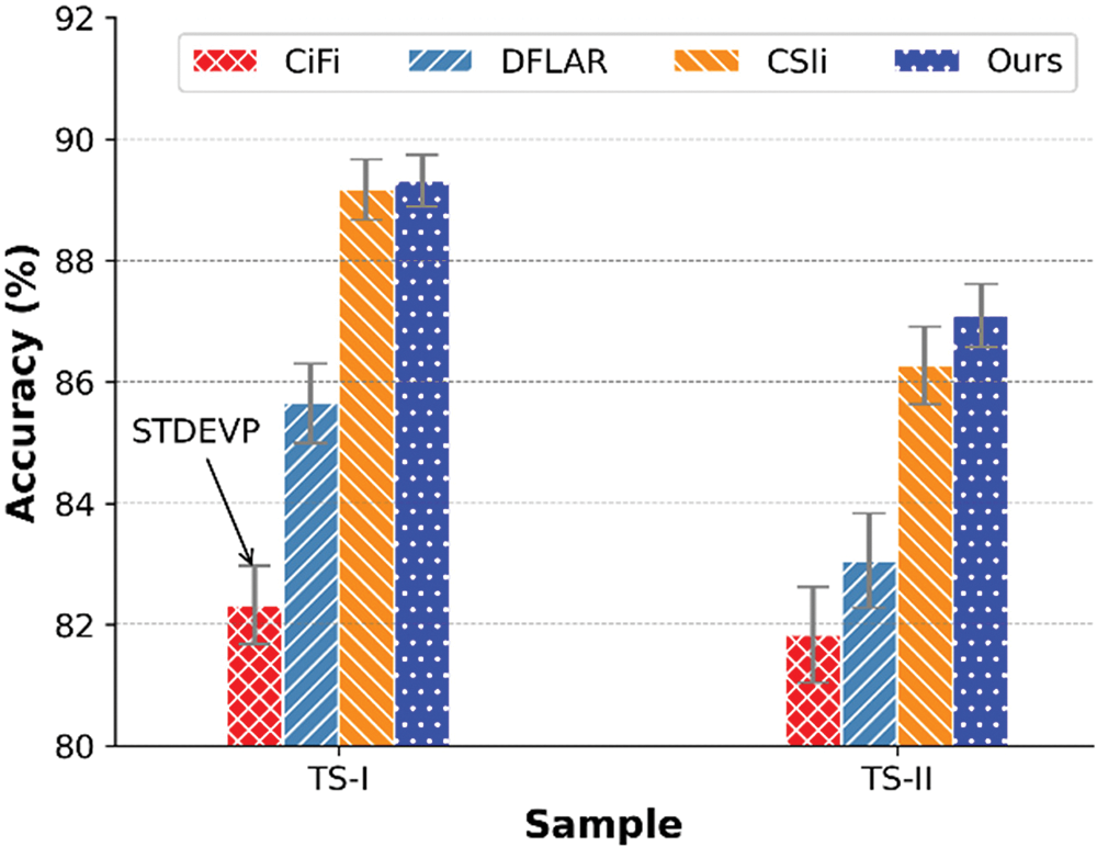
Figure 10: Average accuracy and STDEVP of four methods

6  Conclusion

In this paper, we proposed an input generation scheme for the ML-based Wi-Fi sensing technology. Under the premise of verifying the spatial-temporal-frequency correlation of CSI, we used a novel low-rank matrix factorization algorithm and gradient calculation to generate a multidimensional tensor, which can be fed to the ML-based models for training or performing sensing tasks. We evaluated the proposed method on the case of device-free localization. Experimental results demonstrated its efficiency and outperformed several state-of-the-art method.

In our future work, we will study the specific sensing applications of the proposed method, and explore excellent DL models for different tasks, as well as the sensing problems in multi-TX/RX scenarios.

Acknowledgement: The authors are grateful to the reviewers and editors for helpful suggestions that greatly improved the technical level and logical organization of this paper.

Funding Statement: This work was supported in part by the National Natural Science Foundation of China under Grant 61771258 and Grant U1804142, in part by the Key Science and Technology Project of Henan Province under Grants 202102210280, 212102210159, 222102210192, 232102210051, and in part by the Key Scientific Research Projects of Colleges and Universities in Henan Province under Grant 20B460008.

Author Contributions: The authors confirm contribution to the paper as follows: study conception and design: Liufeng Du, Linghua Zhang, Shaoru Shang; data collection: Shaoru Shang, Xiyan Tian; model building and debugging: Chong Li, Jianing Yang; analysis and interpretation of results: Liufeng Du, Shaoru Shang, Linghua Zhang; draft manuscript preparation: Liufeng Du, Shaoru Shang. All authors reviewed the results and approved the final version of the manuscript.

Availability of Data and Materials: The experimental data in this study were collected by ourselves (see Section 5.1). The data is only used within the research team at present, and the captions and tags these data have not yet been standardized and may not be clear to others. So we plan to release this dataset after it is standardized.

Conflicts of Interest: The authors declare that they have no conflicts of interest to report regarding the present study.

References

1. Xiao, J., Zhou, Z., Yi, Y., Ni, L. M. (2016). A survey on wireless indoor localization from the device perspective. ACM Computing Surveys, 49(2), 1–31. [Google Scholar]

2. Ma, Y., Zhou, G., Wang, S. (2019). WiFi sensing with channel state information: A survey. ACM Computing Surveys, 52(3), 1–36. [Google Scholar]

3. Yan, J., Wan, L., Wei, W., Wu, X., Zhu, W. P. et al. (2021). Device-free activity detection and wireless localization based on CNN using channel state information measurement. IEEE Sensors Journal, 21(21), 24482–24494. [Google Scholar]

4. Yang, Z., Zhou, Z., Liu, Y. (2013). From RSSI to CSI: Indoor localization via channel response. ACM Computing Surveys, 46(2), 1–32. [Google Scholar]

5. Halperin, D., Hu, W., Sheth, A., Wetherall, D. (2010). Predictable 802.11 packet delivery from wireless channel measurements. ACM SIGCOMM Computer Communication Review, 40(4), 159–170. [Google Scholar]

6. Youssef, M., Mah, M., Agrawala, A. (2007). Challenges: Device-free passive localization for wireless environments. Proceedings of the 13th Annual ACM International Conference on Mobile Computing and Networking, pp. 222–229. New YorK, NY, USA. [Google Scholar]

7. Wu, D., Zeng, Y., Zhang, F., Zhang, D. (2022). WiFi CSI-based device-free sensing: From Fresnel zone model to CSI-ratio model. CCF Transactions on Pervasive Computing and Interaction, 4, 88–102. [Google Scholar]

8. Li, Z., Rao, X. (2021). Toward long-term effective and robust device-free indoor localization via channel state information. IEEE Internet of Things Journal, 9(5), 3599–3611. [Google Scholar]

9. Wang, X., Wang, X., Mao, S. (2018). Deep convolutional neural networks for indoor localization with CSI images. IEEE Transactions on Network Science and Engineering, 7(1), 316–327. [Google Scholar]

10. Wang, Z., Huang, Z., Zhang, C., Dou, W., Guo, Y. et al. (2021). CSI-based human sensing using model-based approaches: A survey. Journal of Computational Design and Engineering, 8(2), 510–523. [Google Scholar]

11. Zhang, D., Ma, J., Chen, Q., Ni, L. M. (2007). An RF-based system for tracking transceiver-free objects. Proceedings of the 5th Annual IEEE International Conference on Pervasive Computing and Communications, pp. 135–144. White Plains, NY, USA. [Google Scholar]

12. Xiao, J., Wu, K., Yi, Y., Wang, L., Ni, L. M. (2013). Pilot: Passive device-free indoor localization using channel state information. Proceedings of the IEEE 33rd International Conference on Distributed Computing Systems, pp. 236–245. Philadelphia, PA, USA. [Google Scholar]

13. Sabek, I., Youssef, M. (2013). MonoStream: A minimal-hardware high accuracy device-free WLAN localization system. arXiv Preprint arXiv:1308.0768. [Google Scholar]

14. Qian, K., Wu, C., Yang, Z., Yang, C., Liu, Y. (2016). Decimeter level passive tracking with WiFi. Proceedings of the 3rd Workshop on Hot Topics in Wireless, pp. 44–48. New York, NY, USA. [Google Scholar]

15. Qian, K., Wu, C., Yang, Z., Liu, Y., Jamieson, K. (2017). Widar: Decimeter-level passive tracking via velocity monitoring with commodity Wi-Fi. Proceedings of the 18th ACM International Symposium on Mobile Ad Hoc Networking and Computing, pp. 1–10. New York, NY, USA. [Google Scholar]

16. Roy, P., Chowdhury, C. (2021). A survey of machine learning techniques for indoor localization and navigation systems. Journal of Intelligent & Robotic Systems, 101, 63. [Google Scholar]

17. Gao, Q., Wang, J., Ma, X., Feng, X., Wang, H. (2017). CSI-based device-free wireless localization and activity recognition using radio image features. IEEE Transactions on Vehicular Technology, 66(11), 10346–10356. [Google Scholar]

18. Zhou, R., Lu, X., Zhao, P., Chen, J. (2017). Device-free presence detection and localization with SVM and CSI fingerprinting. IEEE Sensors Journal, 17(23), 7990–7999. [Google Scholar]

19. Zhou, R., Hao, M., Lu, X., Tang, M., Fu, Y. (2018). Device-free localization based on CSI fingerprints and deep neural networks. Proceedings of the 15th Annual IEEE International Conference on Sensing, Communication, and Networking, pp. 1–9. Hong Kong, China. [Google Scholar]

20. Wei, W., Yan, J., Wu, X., Wang, C., Zhang, G. (2022). CSI fingerprinting for device-free localization: Phase calibration and SSIM-based augmentation. IEEE Wireless Communications Letters, 11(6), 1137–1141. [Google Scholar]

21. Sanam, T. F., Godrich, H. (2020). CoMuTe: A convolutional neural network based device free multiple target localization using CSI. arXiv Preprint arXiv:2003.05734. [Google Scholar]

22. Halperin, D., Hu, W., Sheth, A., Wetherall, D. (2011). Tool release: Gathering 802.11n traces with channel state information. ACM SIGCOMM Computer Communication Review, 41(1), 53–53. [Google Scholar]

23. Xie, Y., Li, Z., Li, M. (2015). Precise power delay profiling with commodity WiFi. Proceedings of the 21st Annual International Conference on Mobile Computing and Networking, pp. 53–64. New York, NY, USA. [Google Scholar]

24. Zhu, H., Xiao, F., Sun, L., Wang, R., Yang, P. (2017). R-TTWD: Robust device-free through-the-wall detection of moving human with WiFi. IEEE Journal on Selected Areas in Communications, 35(5), 1090–1103. [Google Scholar]

25. Li, X., Dong, F., Zhang, S., Guo, W. (2019). A survey on deep learning techniques in wireless signal recognition. Wireless Communications and Mobile Computing, 2019, 1–12. [Google Scholar]

26. Yang, Z., Zhang, Y., Chi, G., Zhang, G. (2022). Hands-on wireless sensing with Wi-Fi: A tutorial. arXiv Preprint arXiv:2206.09532. [Google Scholar]

27. Wright, J., Ganesh, A., Rao, S., Peng, Y., Ma, Y. (2009). Robust principal component analysis: Exact recovery of corrupted low-rank matrices via convex optimization. Proceedings of the 23rd Annual Conference on Neural Information Processing Systems 2009, pp. 2080–2088. Vancouver, B.C., Canada. [Google Scholar]

28. Cai, J. F., Candès, E. J., Shen, Z. (2010). A singular value thresholding algorithm for matrix completion. SIAM Journal on Optimization, 20(4), 1956–1982. [Google Scholar]

29. Beck, A., Teboulle, M. (2009). A fast iterative shrinkage-thresholding algorithm for linear inverse problems. SIAM Journal on Imaging Sciences, 2(1), 183–202. [Google Scholar]

30. Lin, Z., Chen, M., Ma, Y. (2010). The augmented lagrange multiplier method for exact recovery of corrupted low-rank matrices. arXiv Preprint arXiv:1009.5055. [Google Scholar]

31. Boyd, S., Parikh, N., Chu, E., Peleato, B., Eckstein, J. (2011). Distributed optimization and statistical learning via the alternating direction method of multipliers. Foundations and Trends® in Machine Learning, 3(1), 1–122. [Google Scholar]

32. Wang, J., Zhang, X., Gao, Q., Ma, X., Feng, X. et al. (2016). Device-free simultaneous wireless localization and activity recognition with wavelet feature. IEEE Transactions on Vehicular Technology, 66(2), 1659–1669. [Google Scholar]