Algorithm Selection Method Based on Coupling Strength for Partitioned Analysis of Structure-Piezoelectric-Circuit Coupling

1  Introduction

Partitioned analysis has attracted attention for application to coupled problems because of its software modularity [1,2]. One focus in this approach is the development of strongly coupled algorithms [3–9]. For coupled problems with a single coupling of phenomena such as fluid-structure interaction, coupling strength, such as the added mass [2,10,11], can be used to select strongly or weakly coupled algorithms [12–14] for the partitioned analysis. In contrast, for coupled multiphysics problems with k types of coupling, k-tuples of a set S that has n elements of coupling formulations can represent possible partitioned algorithms, where the number of k-tuples (maximum number of partitioned algorithms) is nk. The present study proposes a selection method for partitioned algorithms in the coupled multiphysics problem.

Some miniaturized electromechanical systems use energy harvesting based on electromagnetic, electrostatic, or piezoelectric transduction as their electric power supply. Piezoelectric energy harvesting has received the most interest [15]. In a piezoelectric energy harvester, strong structure-piezoelectric-circuit coupling, which determines the frequency response characteristics, can occur. Hence, accurate prediction of the electromechanical behavior is important for the design of such devices. The electromechanical behavior of typical piezoelectric energy harvester models, such as a uniformly laminated thin straight cantilevered composite, has been extensively studied [16]. However, in some cases direct numerical modeling is required for accurate prediction, even for such simple models [17–19]. Here, the term direct means that, prior to the finite element discretization, the governing equations are not transformed into a different form [20]. Direct numerical modeling is required to predict the electromechanical behavior of most advanced energy harvesting systems in terms of geometry complexity, materials, and electrode configuration. Hence, this study focuses on direct numerical modeling.

Previous studies on direct numerical modeling [21] have proposed a monolithic method for structure-piezoelectric-circuit coupling. This method has been recently extended to fluid-structure-piezoelectric-circuit coupling [22]. A partitioned method has been proposed for the direct numerical modeling of structure-piezoelectric-circuit coupling [9]. In these studies, the solution algorithms use fully implicit coupling formulations. That is, in [21,22], the coupling conditions were directly incorporated into the whole coupled equation system, and in [9], the governing equation system for each domain is solved iteratively in the coupling iteration such that the coupling conditions among this domain and other domains are satisfied. Structure-piezoelectric-circuit coupling includes two types of coupling or inverse and direct piezoelectric coupling and direct piezoelectric and circuit coupling. Explicit and implicit formulations are available for these types of coupling. Mixing these formulations leads to variations in partitioned algorithms. A semi-implicit coupling concept for fluid-structure interaction [23] can give further variations. However, only algorithms that use fully implicit coupling formulations are available for the direct numerical modeling of structure-piezoelectric-circuit coupling.

In this study, we propose a coupling-strength-based selection method for the partitioned analysis of structure-piezoelectric-circuit coupling, where an algorithm that uses an implicit and explicit formulation for strong and weak coupling, respectively, is selected to achieve computationally efficient analysis. Based on this selection, three feasible partitioned algorithms are generated from the tuples of the implicit and explicit formulations for the two types of coupling, namely (1) a fully strongly coupled algorithm that uses a fully implicit formulation for both types of coupling, (2) a fully weakly coupled algorithm that uses a fully explicit formulation for both types of coupling, and (3) a partially strongly coupled and partially weakly coupled algorithm that uses an implicit formulation and an explicit formulation for the two types of coupling, respectively. Numerical examples using a circuit-connected piezoelectric oscillator, which is a typical structure-piezoelectric-circuit coupling problem, are used to demonstrate that the proposed method selects a computationally efficient algorithm.

2  Coupling-Strength-Based Selection of Partitioned Algorithms for Structure-Piezoelectric-Circuit Coupling

2.1 Governing Equations

We consider a circuit-connected piezoelectric oscillator as a general model for piezoelectric electromechanical devices. The piezoelectric oscillator and the electric circuit are connected to each other via electrodes. This oscillator can include metal substructures. The electrodes and metal substructures are considered to be a pseudo-piezoelectric material [18], such that the electromechanical behavior of the circuit-connected piezoelectric oscillator is governed by the same equations as those for structure-piezoelectric-circuit coupling.

The piezoelectricity of the material can be described as

σij,j+fi=ρu¨i(1)

Di,i=0(2)

where σij is the ij-th component of the mechanical stress tensor; fi, üi, and Di are the i-th components of the body force, mechanical acceleration, and electric displacement vectors, respectively; and ρ is the mass density. The constitutive equations for the linear piezoelectricity are

σij=CijklESkl−ekijEk(3)

Di=eiklSkl+εikSEk(4)

where Cijkl is the ijkl-th component of the elastic tensor; eijk is the ijk-th component of the piezoelectric constant tensor; Sij and εij are the ij-th components of the mechanical strain and dielectric constant tensors, respectively; and Ei is the i-th component of the electric field vector. The superscripts E and S denote that the quantities are determined under constant electric and strain fields, respectively. Sij is given as (ui,j + uj,i)/2, and Ei is given as −φ,i, where ui is the i-th component of the mechanical displacement vector, and φ is the electric potential. The elementary boundary conditions are the prescribed displacement and electric potential, and the natural boundary conditions are the prescribed surface force and charge.

Eqs. (1)–(4) are spatially discretized using the standard finite element procedure [20]. The matrix-vector form equations of motion for linear piezoelectricity are derived in the global coordinate system as

Muuu¨+Kuuu+Kuφφ=fe(5)

KuφTu+Kφφφ=qe+qc(6)

where Muu is the global matrix of the structural mass; Kuu, Kuφ, and Kφφ are the global matrices of the mechanical, piezoelectric, and dielectric stiffness, respectively; u and φ are the nodal global state variable vectors for the mechanical displacement and electric potential; f and q are the nodal global equivalent vectors for the mechanical external force and charge, respectively; and the subscript e and c denote “external” and “circuit”, respectively.

The electrical resistive load is considered to be the circuit. The electrical behavior can be described using Kirchhoff’s law as

RQ˙+Vp=Ve(7)

where R is the electric resistance, Q is the charge of the electricity, Vp is the electric potential gap between the electrodes given by the piezoelectric material, and Ve is the electric voltage given by the external supply.

Under the assumption of an instantaneous distribution of the circuit charge throughout each electrode, the continuities of the electric potential and charge between the piezoelectric continuum and the electric circuit can be formulated as

qc=∫S+cNφ(Q/S+c)dS−∫S−cNφ(Q/S−c)dS(8)

Vp=φ+∗−φ−∗(9)

where φx* denotes the electric potential at a point where the circuit is connected in the area of the electrode Sxc (x is +, which corresponds to the positive pole, or −, which corresponds to the negative pole); and Nφ is the global assemblage of the shape functions of the electric potential.

2.2 Algorithm Selection Based on Coupling Strength

In the proposed coupling-strength-based selection of partitioned algorithms for structure-piezoelectric-circuit coupling, an algorithm that uses an implicit formulation for strong coupling and an explicit formulation for weak coupling is selected to achieve computationally efficient analysis. Based on this selection, feasible partitioned algorithms are generated from the tuples of the implicit and explicit formulations for the two types of coupling. The coupling condition that corresponds to inverse and direct piezoelectric coupling is satisfied if the following coupling terms in governing Eqs. (5) and (6) are accurately evaluated:

Kuφφand KuφTu(10)

while the coupling condition that corresponds to direct piezoelectric and circuit coupling is satisfied if the following coupling terms in governing Eqs. (6) and (7)are accurately evaluated:

qcand Vp(11)

First, we present the fully strongly coupled algorithm that uses a fully implicit formulation for both types of coupling. In the proposed coupling-strength-based selection method, this algorithm is selected in the case where both the inverse and direct piezoelectric coupling, and the direct piezoelectric and circuit coupling are strong. Note that this algorithm was proposed in a previous study [9], where the in-house code was developed and verified using the benchmark problems. In this study, this code was used to implement the following new algorithms. Second, we propose the partially strongly coupled and partially weakly coupled algorithm that uses an implicit formulation and an explicit formulation for the two types of coupling, respectively. In the proposed coupling-strength-based selection method, this algorithm is selected in the case where the inverse and direct piezoelectric coupling is strong and the direct piezoelectric and circuit coupling is weak. Finally, we propose the fully explicit algorithm that uses a fully explicit formulation for both types of coupling. In the proposed coupling-strength-based selection method, this algorithm is selected in the case where both the inverse and direct piezoelectric coupling and the direct piezoelectric and circuit coupling are weak.

2.3 Partitioned Algorithms for Structure-Piezoelectric-Circuit Coupling

2.3.1 Algorithm 1: Fully Strongly Coupled Algorithm Using Fully Implicit Formulation for Both Types of Coupling

The governing equations for structure-piezoelectric-circuit coupling (5)–(7) are temporally discretized at current time t+Δt such that all the coupling conditions are satisfied; that is, all the coupling terms in Eqs. (10) and (11) are evaluated at current time t+Δt as follows:

Muut+Δtu¨+Kuut+Δtu+Kuφt+Δtφ=t+Δtfe(12)

KuφTt+Δtu+Kφφt+Δtφ=t+Δtqe+t+Δtqc(13)

Rt+ΔtQ˙+t+ΔtVp=t+ΔtVe(14)

The relationships among the mechanical state variables can be given as

t+Δtu˙=tu˙+Δt[γt+Δtu¨+(1−γ)tu¨](15)

t+Δtu=tu+Δttu˙+Δt2[βt+Δtu¨+(1/2−β)tu¨](16)

where β and γ are the control parameters of Newmark’s method. Eq. (12) can be rewritten, using these relationships, as

K^uut+Δtu+Kuφt+Δtφ=t+Δtf^(17)

where

K^uu≡Kuu+(1/βΔt2)Muu(18)

t+Δtf^≡t+Δtfe+(1/βΔt2)Muu[tu+Δttu˙+(1/2−β)Δt2tu¨](19)

The relationship between the electrical state variables is given as

t+ΔtQ=tQ+Δt[(1−γ)tQ˙+γt+ΔtQ˙](20)

where γ is the control parameter of the generalized trapezoidal rule. Eq. (14) can be rewritten using this relationship as

t+ΔtQ=tQ+Δt[(1−γ)tQ˙+γ(t+ΔtVe−t+ΔtVp)/R](21)

The block Gauss–Seidel (BGS) method is used to solve Eqs. (13), (17), and (21)as follows [9]:

K^uut+Δtu(b)=t+Δtf^−Kuφt+Δtφ(b−1)(22)

Kφφt+Δtφ(b)=t+Δtqe+t+Δtqc(b)−KuφTt+Δtu(b)(23)

t+ΔtQ(b)=tQ+Δt{(1−γ)tQ˙+γ(t+ΔtVe−t+ΔtVp(b−1))/R}(24)

where the right-hand superscript b in parentheses denotes the b-th iteration of the BGS loop. Note that t+Δtqc(b) in Eq. (23) and t+ΔtVp(b−1) in Eq. (24) are respectively given by the continuity Eqs. (8) and (9) as

t+Δtqc(b)=∫S+cNφ(t+ΔtQ(b)/S+c)dS−∫S−cNφ(t+ΔtQ(b)/S−c)dS(25)

t+ΔtVp(b−1)=t+Δtφ+∗(b−1)−t+Δtφ−∗(b−1)(26)

The analysis flow of this partitioned algorithm is shown in Fig. 1. As shown, in the BGS loop, the inverse piezoelectric Eq. (22) and the circuit Eq. (24) are solved in parallel, and then the direct piezoelectric Eq. (23) is solved. The BGS loop is then repeated. This algorithm is referred to as Algorithm 1 in Section 3.

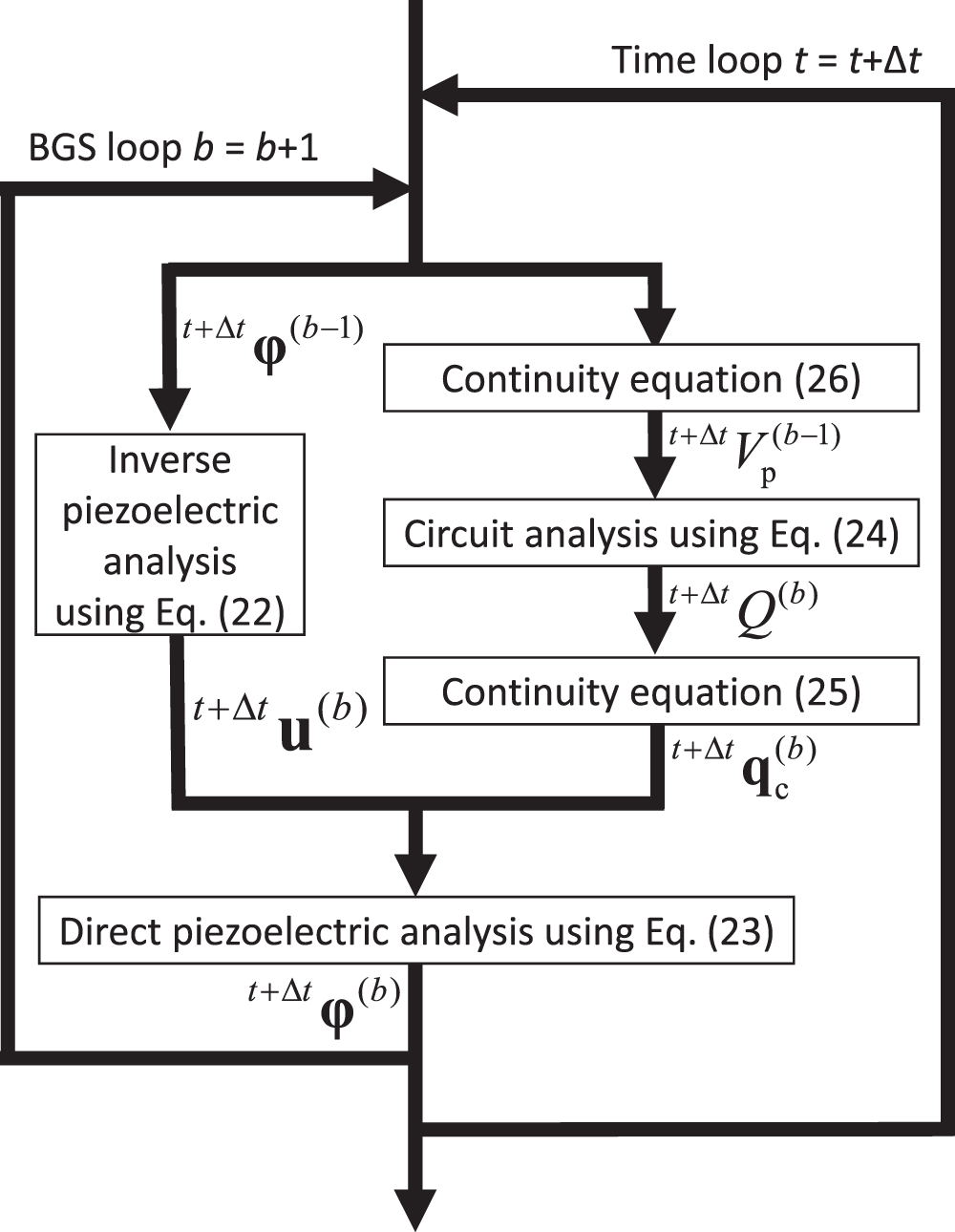
Figure 1: Analysis flow of fully strongly coupled algorithm that uses fully implicit formulation for both types of coupling

The time constant of the corresponding RC circuit is imposed on the time increment for the convergence of the coupled iteration in the fully strongly coupled algorithm (see Section 2.4 for details). From this observation, the forward Euler method can be used for the temporal discretization of the circuit Eq. (7), since it imposes the same constraint on the time increment. Hence, the fully strongly coupled algorithm is changed to the following algorithm, where the coupling condition that corresponds to the direct piezoelectric and circuit coupling is formulated explicitly, or the coupling term Vp in Eq. (11) is predicted using the known value at the previous time step.

2.3.2 Algorithm 2: Partially Strongly Coupled and Partially Weakly Coupled Algorithm that Uses an Implicit Formulation and an Explicit Formulation for the Two Types of Coupling, Respectively

The governing equations for structure-piezoelectric-circuit coupling (5)–(7) are temporally discretized such that all the coupling terms in Eqs. (10) and (11) except Vp are evaluated at current time t+Δt, and Vp is evaluated at previous time t. Then, we obtain Eqs. (12) and (13) and the following equation:

Rt+ΔtQ˙+tVp=t+ΔtVe(27)

By applying the forward Euler method to Eq. (27), this equation is discretized temporally and rearranged as

t+ΔtQ=tQ+Δt(t+ΔtVe−tVp)/R(28)

where tVp is given by the continuity Eq. (9) as

tVp=tφ+∗−tφ−∗(29)

In order to solve Eqs. (12) and (13), the BGS algorithm is used. Eq. (22) is obtained again and Eq. (23) is changed following the explicit formulation for the coupling condition of the direct piezoelectric and circuit coupling as

Kφφt+Δtφ(b)=t+Δtqe+t+Δtqc−KuφTt+Δtu(b)(30)

where t+Δtqc is given by the continuity Eq. (8) as

t+Δtqc=∫S+cNφ(t+ΔtQ/S+c)dS−∫S−cNφ(t+ΔtQ/S−c)dS(31)

in which t+ΔtQ is evaluated using Eq. (28).

The analysis flow of this partitioned algorithm is shown in Fig. 2. As shown, in the time loop, the circuit Eq. (28) is solved, and then in the BGS loop, the inverse piezoelectric Eq. (22) is first solved and then the direct piezoelectric Eq. (30) is solved. The BGS loop is then repeated. This algorithm is referred to as Algorithm 2 in Section 3.

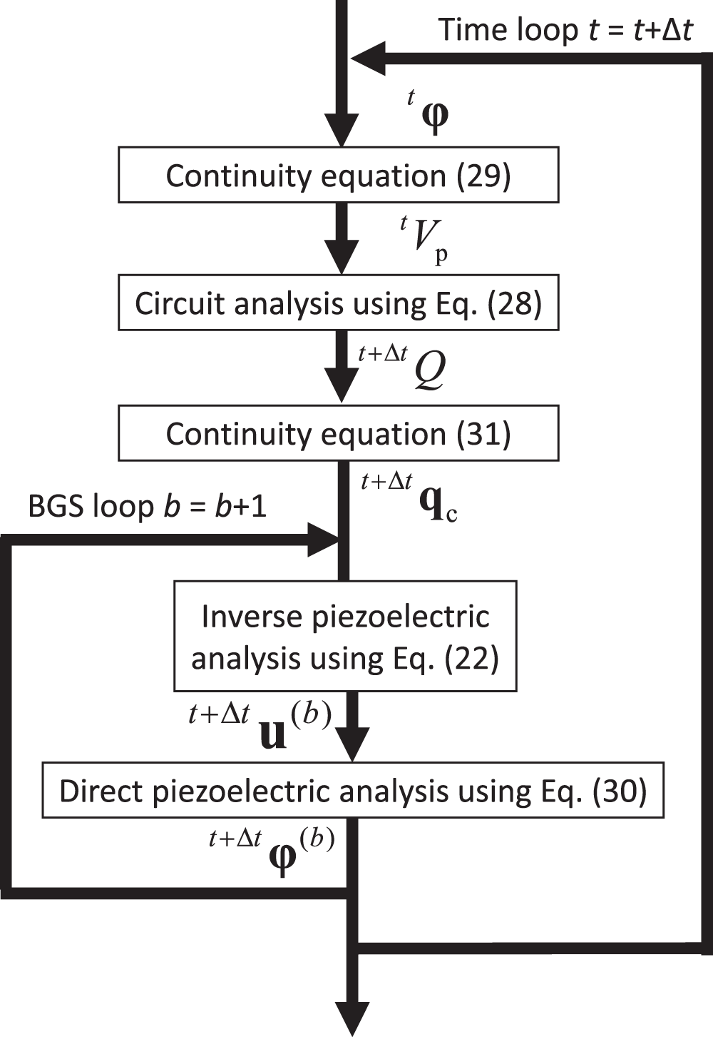
Figure 2: Analysis flow of partially strongly coupled and partially weakly coupled algorithm that uses an implicit formulation and an explicit formulation for the two types of coupling, respectively

2.3.3 Algorithm 3: Fully Weakly Coupled Algorithm that Uses Fully Explicit Formulation for Both Types of Coupling

Kuφφ in the coupling terms in Eq. (10) and Vp in the coupling terms in Eq. (11) are approximated using the known variables at previous time t. Then, Eq. (12) is changed as

Muut+Δtu¨+Kuut+Δtu+Kuφtφ=t+Δtfe(32)

and Eqs. (13) and (27) are obtained, where t+Δtqc in Eq. (13) and tVp in Eq. (27) are respectively given by the continuity Eqs. (8) and (9) as Eqs. (31) and (29). Newmark’s method and the forward Euler method are applied to Eqs. (32) and (27), respectively. These equations reduce to

K^uut+Δtu=t+Δtf^−Kuφtφ(33)

and Eq. (28), respectively. Eq. (13) is rearranged as

Kφφt+Δtφ=t+Δtqe+t+Δtqc−KuφTt+Δtu(34)

The analysis flow of this partitioned algorithm is shown in Fig. 3. As shown, in the time loop, the inverse piezoelectric Eq. (33) and the circuit Eq. (28) are solved in parallel, and then, the direct piezoelectric Eq. (34) is solved. This algorithm is referred to as Algorithm 3 in Section 3.

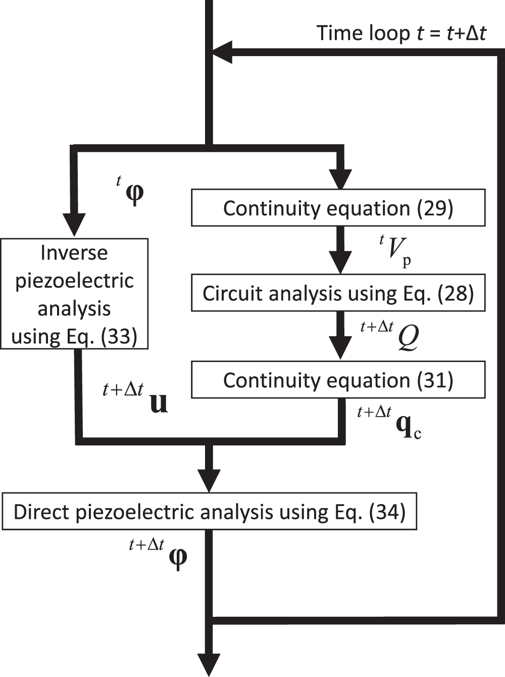
Figure 3: Analysis flow of fully weakly coupled algorithm that uses fully explicit formulation for both types of coupling

2.4 Convergence and Stability

2.4.1 Convergence of Coupling Iteration

When the BGS method is used, the conditions for the convergence of the coupling iteration are required. The coupling iteration for the inverse and direct piezoelectric coupling is considered using the following equations, which are respectively obtained from Eqs. (22) and (23):

K^uut+Δtu(b)+Kuφt+Δtφ(b−1)=0(35)

Kφφt+Δtφ(b)+KuφTt+Δtu(b)=0(36)

After t+Δtu(b) in Eq. (36) is eliminated using Eq. (35), the following recurrence relation is obtained:

t+Δtφ(b)=Λt+Δtφ(b−1)(37)

where the matrix Λ is defined as

Λ≡Kφφ−1KuφTK^uu−1Kuφ(38)

Hence, the necessary condition for convergence is that the maximum modulus of the eigenvalue of the matrix (38) is smaller than 1.

Then, the coupling iteration for the direct piezoelectric and circuit coupling is considered using the following equation, which is obtained from Eqs. (23) and (24):

Cpt+ΔtVp(b)=t+ΔtQ(b)(39)

t+ΔtQ(b)=tQ+Δt{(1−γ)tQ˙−γt+ΔtVp(b−1)/R}(40)

where the piezoelectric structure is reduced to an electrical capacitor element, whose effective capacitance is represented by Cp. Eq. (39) is substituted into Eq. (40) and the resulting equation is rearranged as

t+ΔtQ(b)=tQ+Δt(1−γ)tQ˙−Δtγ/(RCp)t+ΔtQ(b−1)(41)

Hence, the necessary condition for convergence from this equation is given as

|Δtγ/(RCp)|<1or0<Δt<Δtc(42)

where the upper limit RCp/γ is referred to as the critical time increment Δtc.

2.4.2 Stability of Time Marching

First, we consider the stability condition for the time marching that corresponds to the explicit formulation for the direct piezoelectric and circuit coupling. The derived condition is imposed on the time increment used in the partially strongly coupled and partially weakly coupled algorithm and the fully weakly coupled algorithm. The present explicit formulation leads to Eq. (28). In order to consider the stability condition associated with this formulation, Eqs. (30) or (34) is reduced to

Cpt+ΔtVp=t+ΔtQ(43)

where the piezoelectric structure is reduced to an electrical capacitor element with equivalent capacitance Cp. Substituting this equation into Eq. (28) and suitably rearranging the resulting equation gives

t+ΔtQ=(1−Δt/(RCp))tQ(44)

where no external electric power supply is assumed. Hence, the stability condition of the time marching obtained from this equation is given as

|1−Δt/(RCp)|<1or0<Δt<Δtc(45)

where the upper limit 2RCp is referred to as the critical time increment Δtc. Note that the stability condition of the time marching (45) is equivalent to the convergence condition of the coupling iteration (42) if γ = 2 or the Crank-Nicholson method is used in the fully strongly coupled algorithm.

Second, we consider the stability condition of the time marching that corresponds to the fully explicit formulation for both types of coupling or the direct piezoelectric and circuit coupling, and the inverse and direct piezoelectric coupling. Hence, the derived condition is imposed on the fully weakly coupled algorithm. In order to consider the stability condition associated with this formulation, Eqs. (32), (13), and (28) are respectively reduced to

mt+Δta+kt+Δtu−θtVp=0(46)

θt+Δtu+Cpt+ΔtVp=t+ΔtQ(47)

t+ΔtQ=tQ−ΔttVp/R(48)

where the piezoelectric structure is reduced to a SDOF model and the effective system parameters m, k, θ, and Cp are the effective mass, stiffness, electromechanical coupling, and capacitance of the system, respectively. The mechanical external force and the external surface charge are ignored. Eqs. (46) and (48) are respectively reduced using Eq. (47) as

[m0k0]t+ΔtX=[00−θ2/Cpθ/Cp]tX(49)

[0001]t+ΔtX=[00θΔt/(RCp)1−Δt/(RCp)]tX(50)

where X = T[a v u Q]. Similarly, the following relationships are obtained using Newmark’s method:

[−γΔt100]t+ΔtX=[(1−γ)Δt100]t+ΔtX(51)

[−βΔt2010]t+ΔtX=[(1/2−β)Δt2Δt10]t+ΔtX(52)

Eqs. (49)–(52)can be summarized as follows:

At+ΔtX=BtXort+ΔtX=CtX(53)

where the matrices A, B, and C are respectively defined as

A≡[m0k0−γΔt100−βΔt20100001](54)

B≡[00−θ2/Cpθ/Cp(1−γ)Δt100(1/2−β)Δt2Δt1000θΔt/(RCp)1−Δt/(RCp)](55)

C≡A−1B(56)

The matrix C (56) is the amplification matrix. The spectral radius of the amplification matrix can be used to evaluate the stability of the damping vibration analysis. That is, the necessary condition for the stability of the damping vibration analysis is

maxi|λi|≤1(57)

where λi is the i-th eigenvalue of the matrix (56), and |λi| is the modulus of λi.

3  Performance Evaluation and Selection of Partitioned Algorithms Based on Coupling Strength in Shant Damping

Shunt damping is a typical problem of circuit-connected piezoelectric oscillators. When the circuit is an electric resistive load, free mechanical vibrations of the piezoelectric oscillator are damped due to energy consumption as Joule heat in the electric resistive load.

To present the basic capability of the proposed coupling-strength-based selection method, a SDOF model is considered. Then, to demonstrate the generality of the proposed method, a finite element model is considered.

3.1 Single-Degree-of-Freedom Model of Circuit-Connected Piezoelectric Oscillator

3.1.1 Problem Setup

As shown in Fig. 4, a straight rod with a uniform square section is considered. The rod, made of a piezoelectric material, is connected to the electrical resistance via the electrodes that cover the top and bottom surfaces. The inertia and stiffness of the electrodes are negligible, and thus ignored, compared to those of the rod. The rod is fixed at one end and vibrated by a step load applied to the other end.

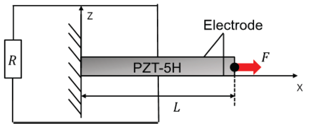
Figure 4: Straight rod with uniform square section made of piezoelectric material

Under the assumption of uniform electromechanical properties in the rod, SDOF modeling respectively reduces the governing Eqs. (5) and (6) to

mu¨+ku−θV=F(58)

θu+CpV=qe+Q(59)

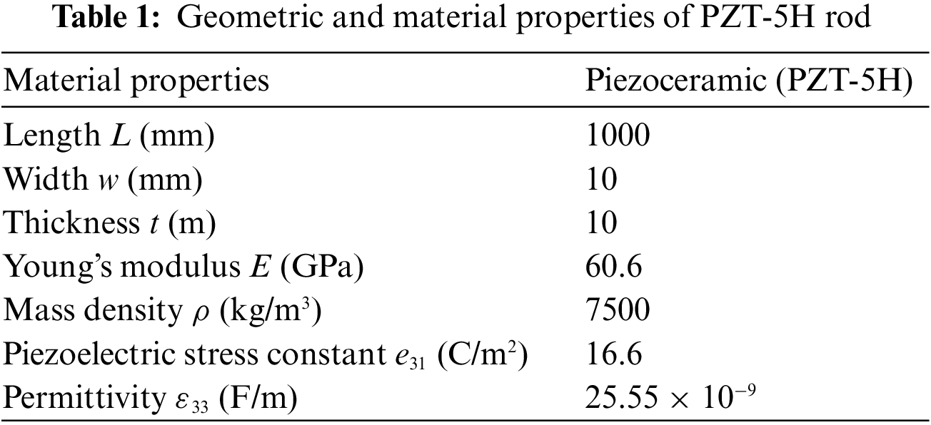
where m, k, θ, and Cp are the mass, spring constant, and coefficients for piezoelectricity and permittivity, respectively, and u, V, F, qe, and Q are the mechanical displacement, electric potential difference, mechanical step load, external charge, and charge from the electric circuit, respectively. The piezoelectric material is PZT-5H. The geometric and material properties of the rod are summarized in Table 1. F is set to 1 N. The electrical resistance R is varied from 10 Ω to 100 MΩ. The case of R = 10 Ω corresponds to a short circuit, and the case of R = 100 MΩ corresponds to an open circuit.

The base time increment Δtbase is set to 0.1 μs, which is about 20% of the critical time increment Δtc = 2RCp in Eqs. (42) or (45) for R = 10 Ω. The relative difference between the solutions obtained using Δtbase and 0.1 × Δtbase is less than 1%. Hence, we can consider the numerical solution obtained using Δtbase to be the convergent solution.

3.1.2 Results and Discussion

First, the numerical solution accuracy is discussed. Fig. 5 shows the relationship between the resistive load and the damping ratio in the mechanical displacement time histories for Algorithms 1, 2, and 3 using Δtbase. As shown, these algorithms produce the same relationship. Note that Algorithm 1 was validated in the previous study [9], and the comparison between Algorithm 1 and the others using the frequency response function can give the typical demonstration of the analysis accuracy. From this figure, the matching impedance was numerically determined to be R = 12 kΩ. That is, R = 12 kΩ maximizes the damping ratio in both Algorithms 1 and 2. This numerical result is very close to the theoretical solution R = 13.1 kΩ, which was given by the following equation [24]:

(ωCpR)opt=1/1+k2(60)

where the natural frequency for impedance matching ω, Cp, and the effective electromechanical coupling coefficient k2 are 2.957 × 103 rad/s, 2.555 × 10−8 F, and 1.2 × 10−1, respectively. Hence, the numerical results obtained using Algorithms 1, 2, and 3 are sufficiently accurate.

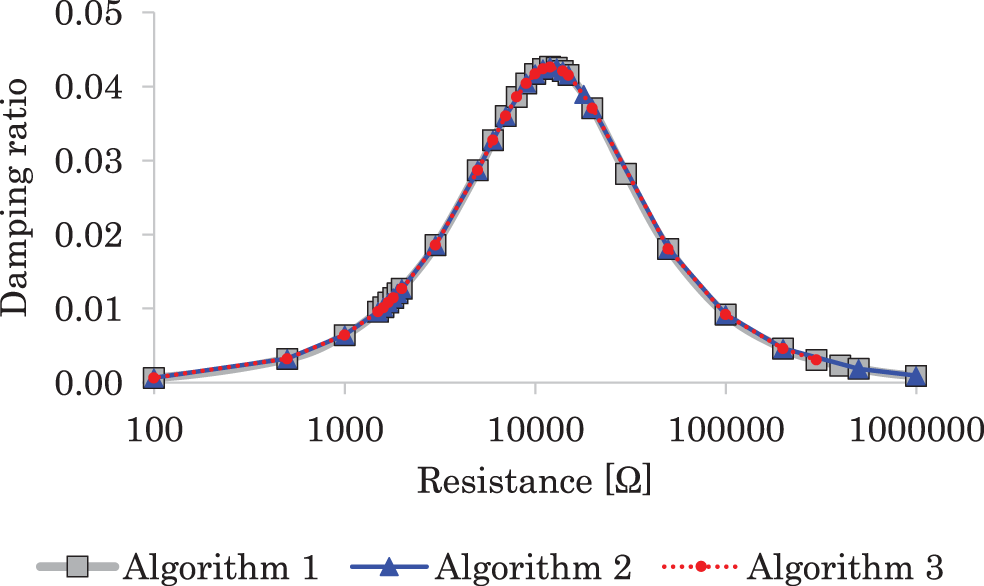
Figure 5: Relationship between resistance and damping ratio for shunt damping problem (SDOF model of circuit-connected piezoelectric oscillator)

Second, the numerical stability is discussed. We used the impedance matching case of R = 12 kΩ here. Table 2 shows the relationship between the time increment Δt and the maximum |λi| in Eq. (57). As shown, the critical time increment for Algorithm 3 is 6.0 × 10−4 to 7.0 × 10−4 s. Fig. 6 shows the mechanical displacement time histories for Algorithm 3 obtained using these time increments. As shown in Fig. 6a, damped free vibration due to shunt damping was obtained for Δt = 6.0 × 10−4 s, and as shown in Fig. 6b, numerical instability was obtained for Δt = 7.0 × 10−4 s. Hence, the stability condition for Algorithm 3 using Eq. (57) is valid. Note that the critical time increment Δtc given by Eq. (46) is 6.1 × 10−4 s, which is consistent with the result obtained using Eq. (57).

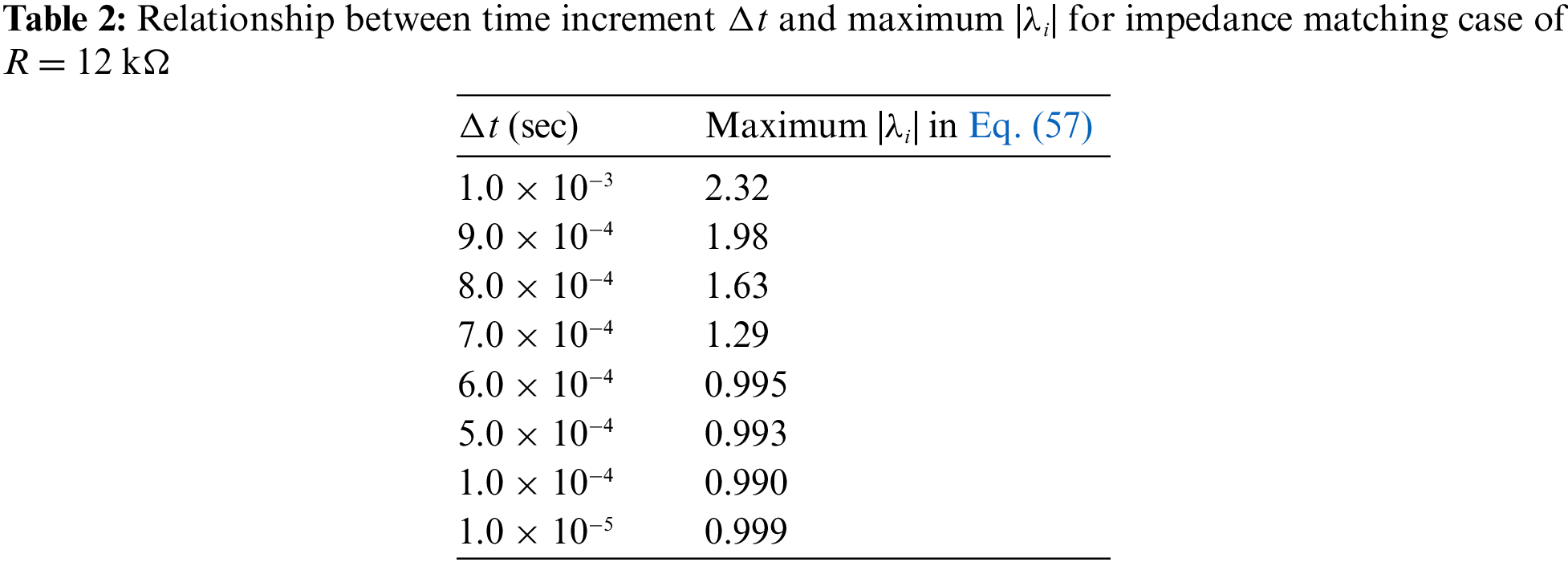
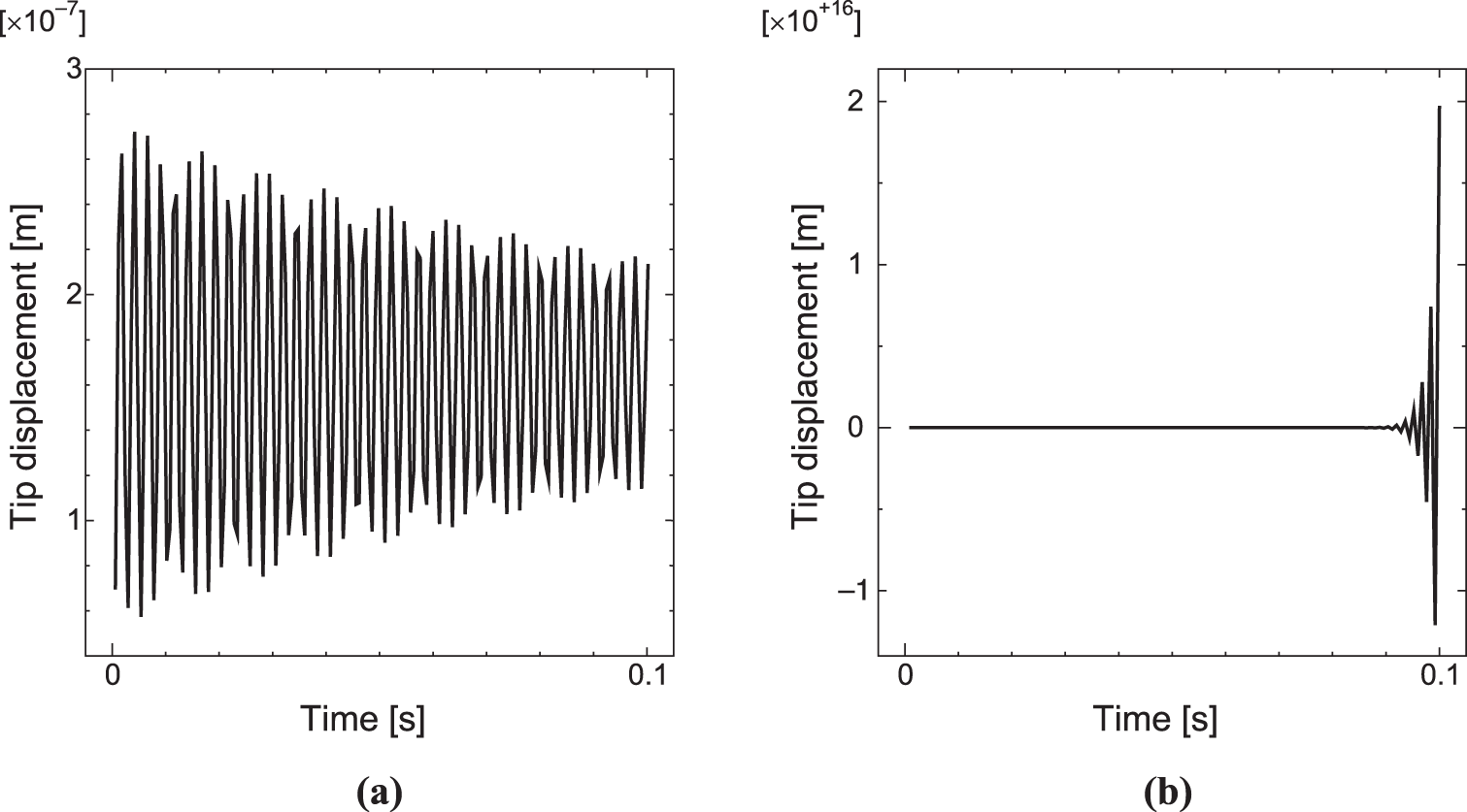
Figure 6: Time histories of mechanical displacement using Algorithm 3 with Δt = (a) 6.0 × 10−4 s, which is smaller than Δtbase, and (b) 7.0 × 10−4 s, which is larger than Δtbase

Finally, the computational cost is discussed. Here, the computational cost Nc is defined as

Nc=Nb×Nt,(61)

where Nb is the number of iterations of the BGS loop, and Nt is the inverse of the time increment Δt*, which can minimize Nc while maintaining sufficient accuracy. Note that Nb for Algorithm 3 is defined as 1. In this study, Δt* is determined using the following algorithm:

•   Increase Δt from Δtbase = 0.1 μs in increments of 0.01 μs (Δt = 0.11, 0.12, 0.13 μs, …) and obtain the mechanical displacement time history for each Δt.

•   Find Δt to minimize Nc while maintaining the relative error of the damping ratio between the results obtained using Δt and Δtbase at less than 1%.

Figs. 7a–7c respectively show the relationship between R and Nb, that between R and Δt* (= 1/Nt), and that between R and Nc (= Nb × Nt).

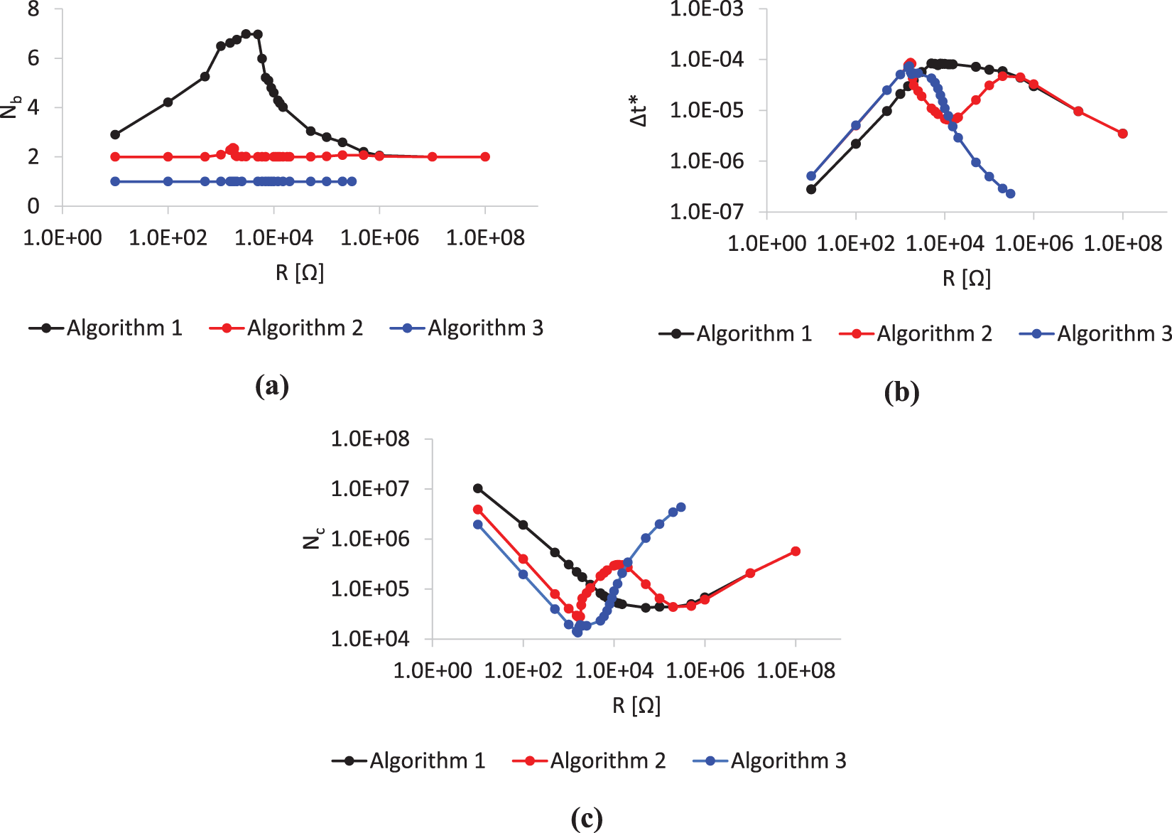
Figure 7: Relationship between electric resistance and number of iterations of (a) BGS loop, (b) time increment Δt*, and (c) computational cost

The strength of the inverse and direct piezoelectric coupling changes with R as follows. For R → 0 (short circuit), there is no coupling because the top and bottom electrodes have the same electric potential. For R → +∞ (open circuit), the coupling strength is maximum because there is no voltage drop at the electric resistance. The coupling strength increases monotonically as R increases between these two extremes. The strength of the direct piezoelectric and circuit coupling changes with R as follows. There is no coupling at the two extremes of R→0 and ∞ because there is no electric current in the circuit. The coupling strength is maximum in the impedance matching case because of the maximum shunt damping. Hence, the proposed coupling-strength-based selection method selects Algorithm 1 in the vicinity of the impedance matching case, Algorithm 2 for large R, and Algorithm 3 for small R. These selections are consistent with the relationship between R and the computational cost shown in Fig. 7c.

As shown in Fig. 7a, Nb for Algorithm 1 is larger than those for the other algorithms for any electrical resistance. This is because Algorithm 1 satisfies two coupling conditions, whereas the other algorithms satisfy only one or no coupling condition in the BGS iteration. However, as shown in this figure, Nb values for all algorithms are comparable. In contrast, as shown in Figs. 7b and 7c, Δt* and Nc are strongly correlated with each other. Hence, the algorithm selection is discussed based on the relationship between R and Δt* as follows.

In the small-resistance region, Algorithm 3 is selected since the computational cost is minimum, as shown in Fig. 7c. As shown in Fig. 7b, Δt* for all algorithms monotonically increases as R increases in this region, since the critical time increment Δtc imposed on Δt* is proportional to R. Hence, Nc monotonically decreases in this region. After this region, Δt* for Algorithm 2 decreases drastically as R increases. Δt* for Algorithm 2 is minimum in the impedance matching case of R = 12 kΩ, and increases again after this R value until it reaches Δt* for Algorithm 1. The strength of the direct piezoelectric and circuit coupling is maximum in the impedance matching case because of the shunt damping. Hence, the decrease of Δt* for Algorithm 2 is due to the direct piezoelectric and circuit coupling, which is explicitly formulated in Algorithm 2. The behavior of Δt* for Algorithm 3 is similar to that for Algorithm 2, since the direct piezoelectric and circuit coupling is also explicitly formulated in Algorithm 3. However, different from Algorithm 2, Δt* for Algorithm 3 decreases continuously as R increases beyond the impedance matching case. This is because the strength of the inverse and direct piezoelectric coupling increases as R increases, and, different from Algorithm 2, this coupling is explicitly formulated in Algorithm 3.

In the vicinity of the impedance matching case, Algorithm 1 is selected, since the computational cost is minimum as shown in Fig. 7c. In this region, the inverse and direct piezoelectric coupling and the direct piezoelectric and circuit coupling are strong. Both types of coupling are formulated implicitly in Algorithm 1. Hence, Algorithm 1 is most computationally efficient in this region.

In the large-resistance region, as shown in Fig. 7c, the computational efficiencies of Algorithms 1 and 2 are almost equivalent, and that of Algorithm 3 degrades as R increases. In this region, the inverse and direct piezoelectric coupling is strong and the piezoelectric and circuit coupling is weak. Hence, Algorithm 2 is selected.

3.2 Finite Element Model of Circuit-Connected Piezoelectric Oscillator

3.2.1 Problem Setup

As shown in Fig. 8, an energy harvester that uses a piezoelectric material is typically modeled as a symmetric bimorph cantilevered beam with three layers. The outer two piezoelectric layers are oppositely poled in the out-of-plane direction. The metal substructure, which is the intermediate layer between the piezoelectric layers, is made of brass. The electrodes on the opposite faces of the piezoelectric layers are set to be much thinner than the overall thickness and are connected to the resistive load. The cantilever is initially subjected to bending deformation, whose magnitude at the tip is set to utip = 2.0 μm. The substructure and electrodes are modeled as a pseudo-piezoelectric material, whose piezoelectric constant matrix e is set to 0 and dielectric constant matrix ε is set to 1, such that the whole system can be analyzed using a single numerical procedure [18]. The geometric and material properties of the piezoelectric, substructure, and electrode layers are summarized in Table 3. Mixed interpolation of tensorial components shell elements [25,26] and hexahedral quadratic 20-node solid elements are used for the inverse and direct piezoelectric analyses, respectively, using the degrees of freedom transformation between solid and shell elements [27]. The reason why these elements are used is the shell element is efficient and accurate for the thin plate bending analysis, while the solid element is necessary for describing the three-dimensional distribution of the electric quantity in the piezoelectric continuum. The numbers of in-plane mesh divisions of the cantilever are 10 and 1, respectively, along the longitudinal and width directions. The numbers of divisions of the solid mesh along the thickness direction are 3 for each piezoceramic layer, 2 for the intermediate layer, and 1 for each electrode layer. γ = 0.5 is used in the time integration method, which corresponds to the Crank–Nicholson method. Δtbase is set to 1.0 × 10−6 s, which is about 25% of Δtc in Eqs. (42) and (45) using R = 470 Ω.

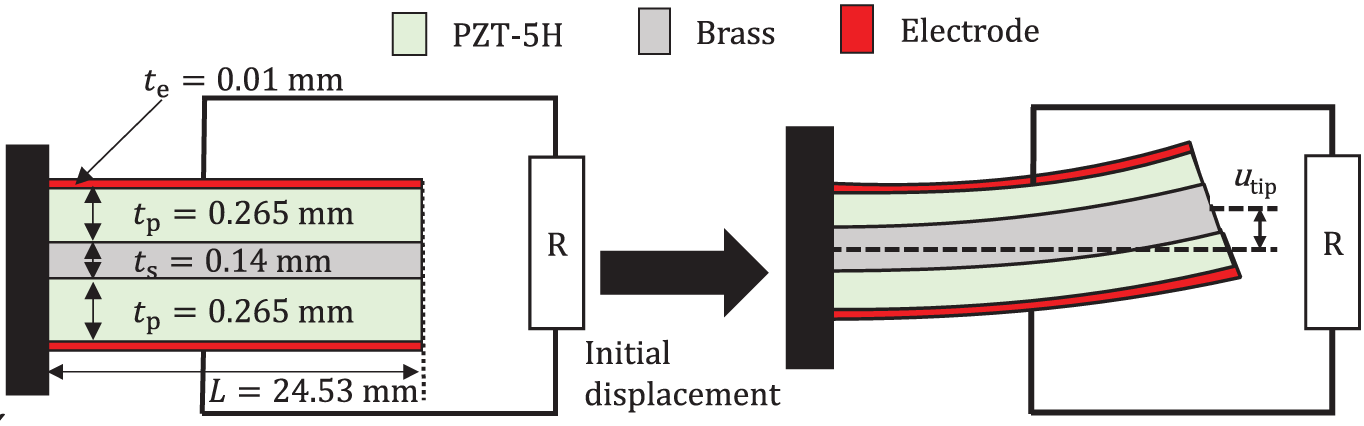
Figure 8: Bimorph cantilever energy harvester

3.2.2 Results and Discussion

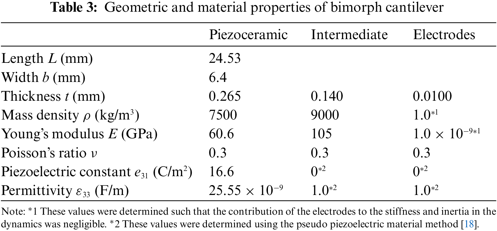
Fig. 9 shows the time histories of the tip bending displacement of the bimorph obtained using Algorithms 1 and 2. As shown, shut damping appears for all cases of R. This energy consumption is most significant in the impedance matching case (Fig. 9b). Fig. 10 shows the relationships between the resistive load and the damping ratio in the time histories of the tip bending displacement obtained using Algorithms 1 and 2 with Δtbase. As shown, these algorithms produce the same relationship. Note that Algorithm 1 was validated in the previous study [9], and the comparison between Algorithm 1 and the others using the frequency response function can give the typical demonstration of the analysis accuracy. From this figure, the matching impedance was determined to be 34 kΩ. That is, R = 34 kΩ maximizes the damping ratio in both Algorithms 1 and 2. This numerical result is very close to the theoretical solution R = 37.8 kΩ given by Eq. (60), where ω, Cp, and k2 are 3.281 × 103 rad/s, 7.568 × 10−9 F, and 3.716 × 10−1, respectively. Hence, the numerical results obtained using Algorithms 1 and 2 are sufficiently accurate.

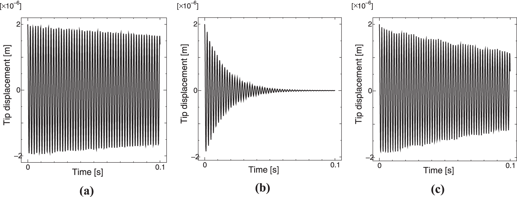
Figure 9: Time histories of tip bending displacement of bimorph for electric resistance values of (a) R = 470 Ω, (b) 34 kΩ, and (c) 995 kΩ

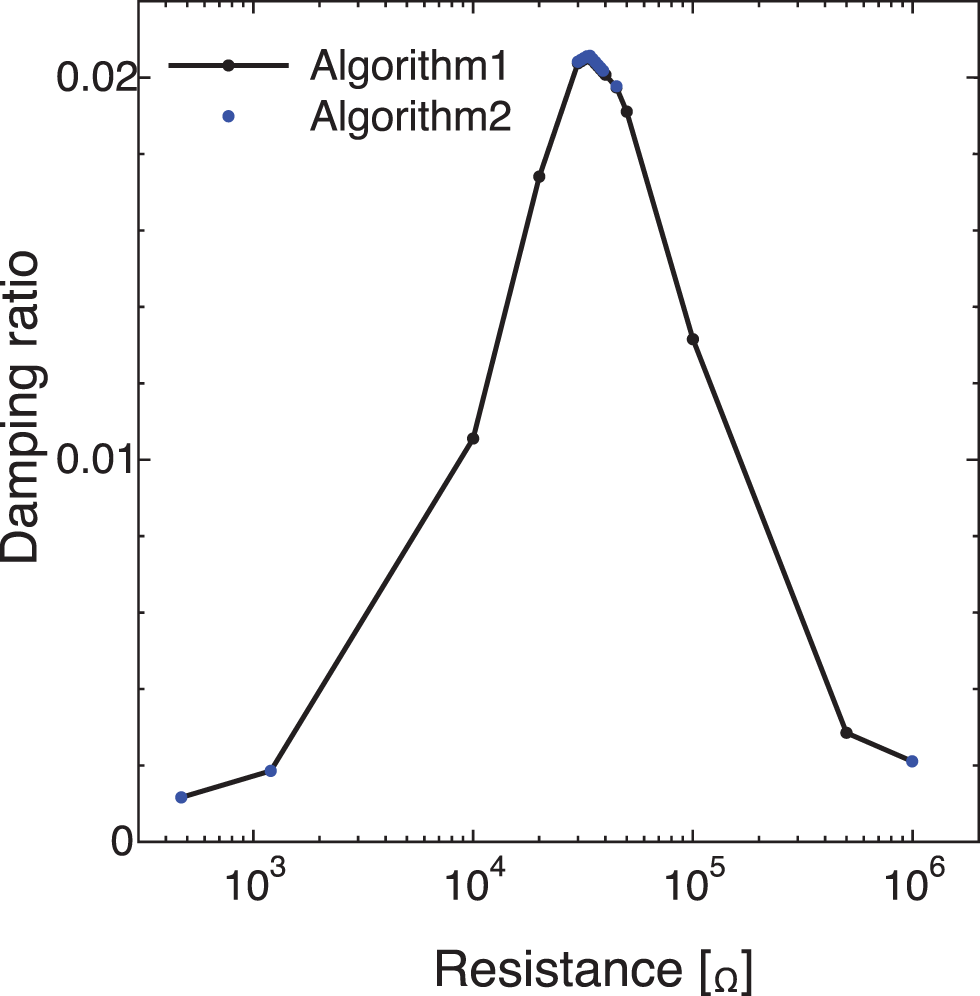
Figure 10: Relationship between resistance and damping ratio for shunt damping problem (finite element model of circuit-connected piezoelectric oscillator)

In contrast, as shown in Fig. 11, numerical instability was observed in the results obtained using Algorithm 3 with Δt equal to or smaller than Δtbase. Note that Δtbase is about 25% of Δtc in Eqs. (42) and (45), which corresponds to the explicit formulation of the direct piezoelectric and circuit coupling. We also examined Δtc obtained using Eq. (57), which corresponds to the explicit formulation of both the inverse and direct piezoelectric coupling, and the direct piezoelectric and circuit coupling. Under the assumption of a first bending mode, the effective system parameters in the governing Eqs. (46)–(48) of a SDOF system can be determined as [28]

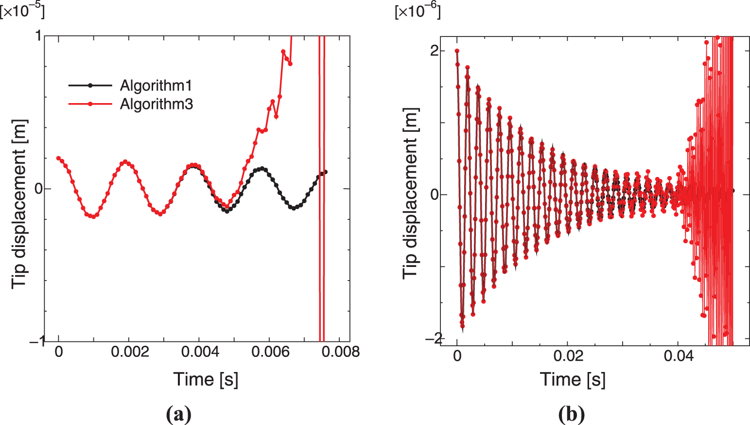
Figure 11: Time histories of mechanical displacement obtained using Algorithm 3 with (a) Δt = Δtbase and R = 34 kΩ and (b) Δt = 0.1 × Δtbase and R = 34 kΩ

m=(ρsts+2ρptp)b(62)

k=[1.0302Es(ts3/L4)+2.0604Ep(3ts2tp+6tstp2+4tp3)/L4]b(63)

θ=−2.753d31Epb(ts+tp)/L3(64)

Cp=2K3sε0bL/tp(65)

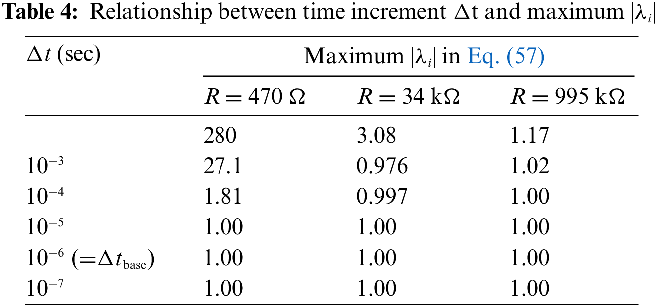
where d31 is the piezoelectric strain constant, K3s is the relative dielectric constant at constant strain, and the subscripts s and p denote the substructure and piezoelectric layers, respectively. The relationship between Δt and the maximum |λi| in Eq. (57) is given in Table 4. As shown, the maximum |λi| is not smaller than 1 for any Δt. Note that this result is an evaluation of numerical stability for first-bending-mode vibration, whereas the finite element model includes higher-mode vibration. Hence, the numerical instability observed in Fig. 11 was caused by higher-mode vibration.

Finally, the computational cost is discussed, which is defined as Nc in Eq. (61). Following this equation, the unit of Nc is the number of computations per unit time. Here, we consider only Algorithms 1 and 2, since Algorithm 3 is unconditionally unstable, as discussed above. Figs. 12a and 12b show the relationship between the electric resistance R and the computational cost Nc for the SDOF model and the finite element model, respectively. As shown, the relationships are very similar. As shown in Fig. 12b, similar to the case for the SDOF model, Algorithm 1 is selected in the vicinity of the impedance matching case and Algorithm 2 is selected in other regions of R. These results confirm that the proposed coupling-strength-based selection method selects the best partitioned algorithm in terms of computational efficiency.

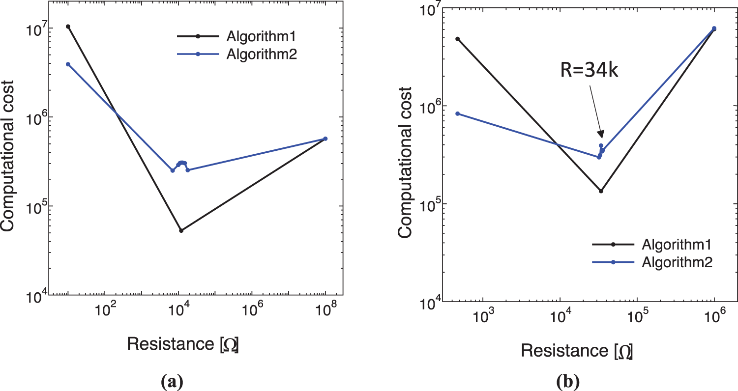
Figure 12: Relationship between electric resistance and computational cost for (a) SDOF model and (b) finite element model

4  Concluding Remarks

In this study, a coupling-strength-based selection method of partitioned algorithms was proposed for structure-piezoelectric-circuit coupling. In the proposed method, implicit and explicit formulations are used for strong and weak coupling, respectively. A coupled multiphysics problem that includes inverse and direct piezoelectric coupling and direct piezoelectric and circuit coupling was considered. In a circuit-connected piezoelectric oscillator, which is a typical structure-piezoelectric-circuit coupling problem, the strength of these two types of coupling changes with the electric resistive load. Hence, we generate three feasible partitioned algorithms based on the proposed coupling-strength-based selection, namely (1) the fully implicit partitioned algorithm (proposed in our previous study), (2) the partially implicit and partially explicit partitioned algorithm (proposed here), and (3) the fully explicit partitioned algorithm (proposed here). In numerical experiments using circuit-connected piezoelectric oscillator models, we evaluated these algorithms in terms of computational efficiency, which was measured using the computational cost. In the small-electric-resistance region, the fully explicit partitioned algorithm or the partially implicit and partially explicit partitioned algorithm is selected since they both explicitly formulate the inverse and direct piezoelectric coupling, which is weak in this region. In the vicinity of the impedance matching case, the fully implicit partitioned algorithm is selected since it implicitly formulates both types of coupling, which are strong in this region. In the large-electric-resistance region, the partially implicit and partially explicit partitioned algorithm is selected since it implicitly formulates the inverse and direct piezoelectric coupling, which is strong, and explicitly formulates the direct piezoelectric and circuit coupling, which is weak. The numerical results clearly demonstrate a consistency between the computational cost and the coupling-strength-based selection. Hence, it can be concluded that the proposed coupling-strength-based selection method effectively selects partitioned algorithms in the coupled multiphysics problem. The proposed method can be used as a framework for designing partitioned algorithms in coupled multiphysics problems. In future work, we will apply this framework to more complicated coupled multiphysics problems such as fluid-structure-piezoelectric-circuit coupling, which should be considered in the design process of flapping-wing nano air vehicles [29–31]. In this multiphysics problem with three types of coupling, 3-tuples of the set S with elements of two or more coupling formulations represent possible partitioned algorithms, where the maximum number of partitioned algorithms is 23 or more. Hence, an algorithm design framework that uses the proposed coupling-strength-based selection method will be important for complicated coupled multiphysics problems.

Acknowledgement: The authors thank the support from the Japan Society for the Promotion of Science.

Funding Statement: This research was supported by the Japan Society for the Promotion of Science, KAKENHI Grant Nos. 20H04199 and 23H00475.

Author Contributions: The authors confirm contribution to the paper as follows: study conception and design: D. Ishihara; data collection: N. Takayama; analysis and interpretation of results: D. Ishihara, N. Takayama; draft manuscript preparation: D. Ishihara. All authors reviewed the results and approved the final version of the manuscript.

Availability of Data and Materials: The datasets analyzed during the current study are available from the corresponding author on reasonable request.

Conflicts of Interest: The authors declare that they have no conflicts of interest to report regarding the present study.

References

1. Dettmer, W., Peric, D. (2006). A computational framework for fluid-structure interaction: Finite element formulation and applications. Computer Methods in Applied Mechanics and Engineering, 195, 5754–5779. https://doi.org/10.1016/j.cma.2005.10.019 [Google Scholar] [CrossRef]

2. Badia, S., Quaini, A., Quarteroni, A. (2008). Modular vs. non-modular preconditioners for fluid-structure systems with large added-mass effect. Computer Methods in Applied Mechanics and Engineering, 197, 4216–4232. https://doi.org/10.1016/j.cma.2008.04.018 [Google Scholar] [CrossRef]

3. Matthies, H. G., Steindorf, J. (2003). Partitioned strong coupling algorithms for fluid-structure interaction. Computers and Structures, 81, 805–812. https://doi.org/10.1016/S0045-7949(02)00409-1 [Google Scholar] [CrossRef]

4. Matthies, H. G., Niekamp, R., Steindorf, J. (2006). Algorithms for strong coupling procedures. Computer Methods in Applied Mechanics and Engineering, 197, 4216–4232. https://doi.org/10.1016/j.cma.2004.11.032 [Google Scholar] [CrossRef]

5. Yamada, T., Yoshimura, S. (2008). Line search partitioned approach for fluid-structure interaction analysis of flapping wing. Computer Modeling in Engineering and Science, 24(1), 51–60. https://doi.org/10.3970/cmes.2008.024.051 [Google Scholar] [CrossRef]

6. Kataoka, S., Minami, S., Kawai, H., Yamada, T., Yoshimura, S. (2014). A parallel iterative partitioned coupling analysis system for large-scale acoustic fluid-structure interactions. Computational Mechanics, 53(6), 1299–1310. https://doi.org/10.1007/s00466-013-0973-1 [Google Scholar] [CrossRef]

7. Hong, G., Kaneko, S., Mitsume, N., Yamada, T., Yoshimura, S. (2021). Robust fluid-structure interaction analysis for parametric study of flapping motion. Finite Elements in Analysis and Design, 183–184, 103494. https://doi.org/10.1016/j.finel.2020.103494 [Google Scholar] [CrossRef]

8. Ramegowda, P. C., Ishihara, D., Takata, R., Niho, T., Horie, T. (2020). Hierarchically decomposed finite element method for a triply coupled piezoelectric, structure, and fluid fields of a thin piezoelectric bimorph in fluid. Computer Methods in Applied Mechanics and Engineering, 365, 113006. https://doi.org/10.1016/j.cma.2020.113006 [Google Scholar] [CrossRef]

9. Ishihara, D., Takata, R., Ramegowda, P. C., Takayama, N. (2021). Strongly coupled partitioned iterative method for the structure-piezoelectric-circuit coupling using hierarchical decomposition. Computers and Structures, 253, 106572. https://doi.org/10.1016/j.compstruc.2021.106572 [Google Scholar] [CrossRef]

10. Forster, C., Wall, W. A., Ramm, E. (2007). Artificial added mass instabilities in sequential staggered coupling of nonlinear structures and incompressible viscous flows. Computer Methods in Applied Mechanics and Engineering, 196, 1278–1293. https://doi.org/10.1016/j.cma.2006.09.002 [Google Scholar] [CrossRef]

11. Idelsohn, S. R., Del Pin, F., Rossi, R., Onate, E. (2009). Fluid-structure interaction problems with strong added-mass effect. International Journal for Numerical Methods in Engineering, 80, 1261–1294. https://doi.org/10.1002/nme.2659 [Google Scholar] [CrossRef]

12. Hua, Z., Maxit, L., Cheng, L. (2019). Mid-to-high frequency piecewise modelling of an acoustic system with varying coupling strength. Mechanical Systems and Signal Processing, 134, 106312. https://doi.org/10.1016/j.ymssp.2019.106312 [Google Scholar] [CrossRef]

13. Egab, L., Wang, X. (2022). On the analysis of coupling strength of a stiffened plate-cavity coupling system using a deterministic-statistical energy analysis method. Mechanical Systems and Signal Processing, 164, 108234. https://doi.org/10.1016/j.ymssp.2021.108234 [Google Scholar] [CrossRef]

14. Fang, C., Zeng, Y., Zhang, Y. (2023). A numerical strategy for predicting the coupling-strength of acoustic fluid-structure interaction. Computers and Structures, 275, 106902. https://doi.org/10.1016/j.compstruc.2022.106902 [Google Scholar] [CrossRef]

15. Priya, S. (2007). Advances in energy harvesting using low profile piezoelectric transducers. Journal of Electroceramics, 19, 167–184. https://doi.org/10.1007/s10832-007-9043-4 [Google Scholar] [CrossRef]

16. Erturk, A., Inman, D. J. (2011). Piezoelectric energy harvesting. The Atrium, Southern Gate, Chichester, West Sussex, PO19 8SQ, England: John Wiley & Sons, Ltd. [Google Scholar]

17. Steel, M. R., Harrison, F., Harper, P. G. (1978). The piezoelectric bimorph: An experimental and theoretical study of its quasistatic response. Journal of Physics D: Applied Physics, 11(6), 979–989. https://doi.org/10.1088/0022-3727/11/6/017 [Google Scholar] [CrossRef]

18. Ramegowda, P. C., Ishihara, D., Takata, R., Niho, T., Horie, T. (2020). Finite element analysis of a thin piezoelectric bimorph with a metal shim using solid direct-piezoelectric and shell inverse-piezoelectric coupling with pseudo direct-piezoelectric evaluation. Composite Structures, 245, 112284. https://doi.org/10.1016/j.compstruct.2020.112284 [Google Scholar] [CrossRef]

19. Ishihara, D., Ramegowda, P. C., Aikawa, S., Iwamaru, N. (2013). Importance of three-dimensional piezoelectric coupling modeling in quantitative analysis of piezoelectric actuators. Computer Modeling in Engineering and Sciences, 136(2), 1187–1206. https://doi.org/10.32604/cmes.2023.024614 [Google Scholar] [PubMed] [CrossRef]

20. Bathe, K. J. (1996). Finite element procedures. Englewood Cliffs, N.J.: Prentice-Hall. [Google Scholar]

21. Ravi, S., Zilian, A. (2017). Monolithic modeling and finite element analysis of piezoelectric energy harvesters. Acta Mechanica, 228, 2251–2267. https://doi.org/10.1007/s00707-017-1830-7 [Google Scholar] [CrossRef]

22. Shang, L., Hoareau, C., Zilian, A. (2022). Modeling and simulation of thin-walled piezoelectric energy harvesters immersed in flow using monolithic fluid-structure interaction. Finite Elements in Analysis and Design, 206, 103761. https://doi.org/10.1016/j.finel.2022.103761 [Google Scholar] [CrossRef]

23. Fernandez, M. A., Gerbeau, J. F., Grandmont, C. (2007). A projection semi-implicit scheme for the coupling of an elastic structure with an incompressible fluid. International Journal for Numerical Methods in Engineering, 69, 794–821. https://doi.org/10.1002/(ISSN)1097-0207 [Google Scholar] [CrossRef]

24. Liao, Y., Sodano, H. A. (2010). Piezoelectric damping of resistively shunted beams and optimal parameters for maximum damping. Vibration and Acoustics, 132(4), 041014. https://doi.org/10.1115/1.4001505 [Google Scholar] [CrossRef]

25. Dvorkin, E. N. (1995). Nonlinear analysis of shells using the MITC formulation. Archives of Computational Methods in Engineering, 2(2), 1–50. https://doi.org/10.1007/BF02904994 [Google Scholar] [CrossRef]

26. Bathe, K. J., Iosilevich, A., Chapelle, D. (2000). An evaluation of the MITC shell elements. Computers and Structures, 75(1), 1–30. https://doi.org/10.1016/S0045-7949(99)00214-X [Google Scholar] [CrossRef]

27. Ramegowda, P. C., Ishihara, D., Niho, T., Horie, T. (2019). A novel coupling algorithm for the electric field-structure interaction using a transformation method between solid and shell elements in a thin piezoelectric bimorph plate analysis. Finite Elements in Analysis and Design, 159, 33–49. https://doi.org/10.1016/j.finel.2019.02.001 [Google Scholar] [CrossRef]

28. Liao, Y., Sodano, H. A. (2012). Optimal placement of piezoelectric material on a cantilever beam for maximum piezoelectric damping and power harvesting efficiency. Smart Materials and Structures, 21, 105014. https://doi.org/10.1088/0964-1726/21/10/105014 [Google Scholar] [CrossRef]

29. Rashmikant, Ishihara D., Suetsugu R., Ramegowda P. C. (2021). One-wing polymer micromachined transmission for insect-inspired flapping wing nano air vehicles. Engineering Research Express, 3(4), 045006. https://doi.org/10.1088/2631-8695/ac2bf0 [Google Scholar] [CrossRef]

30. Ishihara, D. (2022). Computational approach for the fluid-structure interaction design of insect-inspired micro flapping wings. Fluids, 7(1), 26. https://doi.org/10.3390/fluids7010026 [Google Scholar] [CrossRef]

31. Rashmikant, Ishihara, D. (2023). Iterative design window search for polymer micromachined flapping-wing nano air vehicles using nonlinear dynamic analysis. International Journal of Mechanics and Materials in Design, 19(2), 407–429. https://doi.org/10.1007/s10999-022-09635-4 [Google Scholar] [CrossRef]