Tool Wear State Recognition with Deep Transfer Learning Based on Spindle Vibration for Milling Process

1  Introduction

The health monitoring system for the tool can detect the wear state of the tool during the cutting process. It is capable of offering process decision support to engineers or automatic production control systems. The conventional tool monitoring methods establish a tool wear state recognition model that relies on historical cutting conditions. After that, the model can be employed to oversee new cutting tools under identical circumstances. The research conducted in the studies has yielded plentiful research results [1–3]. Especially with the advancement of deep learning technology, models based on deep learning have outperformed traditional models in recognizing the wear state of tools [4,5].

There are two kinds of methods for tool wear monitoring: the direct monitoring method and the indirect monitoring method. The direct monitoring method primarily utilizes machine vision technology for the purpose of measuring tool wear. Zhang et al. obtained tool wear images from the online CCD camera [6]. Qin et al. used a dynamic image sequence for face milling tool wear monitoring [7]. Nevertheless, the measurement that relies on machine vision must be actively involved in the cutting process. The chips and cutting fluid greatly affect the measurement results. Applying it to the production site is a challenging task. The indirect monitoring method establishes a pattern recognition model that recognizes the tool wear status through monitoring signals. Indirect monitoring of tool wear can be achieved through the use of machining signals, which include current signal, vibration signal, acoustic emission signal, and force signal. The cutting force signal can provide direct feedback on the level of tool wear. The downside is that the measurement of cutting force will significantly affect the production process. The measuring equipment is too expensive to be widely utilized. The stress wave generated by chip deformation in the cutting contact area is the acoustic emission signal. Some studies have indicated that the acoustic emission signal can indirectly indicate the tool wear states [8,9]. However, acoustic emission signals place high demands on signal acquisition and storage. Current signals is also utilized to predict tool wear [10,11]. The advantage of this signal is that it is easy to obtain. However, the current signal transmission path is lengthy, causing the loss of high-frequency signals that reflect the change in cutting state. The cutting vibration signal can indicate the contact status between the tool and the workpiece. It possesses the suitable frequency bandwidth. The installation of the acceleration sensor is convenient, and it has been widely utilized by researchers. Kilundu et al. successfully conducted tool condition monitoring in metal cutting through the analysis of vibration signals on a singular spectrum [12]. Stavropoulos et al. investigated the mechanism of generating face milling vibration signals [13]. High spindle speed can blur the time-domain characteristics of vibration signals, making signal analysis and processing greatly difficult.

Researchers have proposed time domain-based methods [14,15], frequency domain-based methods [16,17] and time-frequency domain-based methods [18] for different research purposes in terms of the analysis and processing methods of monitoring signals. The time-domain method utilizes statistical theory to determine the characteristics of signals. It offers advantages such as requiring a small amount of computation and being ideal for real-time monitoring. The features of the domain are highly susceptible to the working conditions. The frequency-domain method is the most widely used analysis method in prognostics and health management. The signal spectrum or envelope spectra [19] comprises substantial vibration source information. In comparison to the amplitude attenuation in the time domain during the propagation process, the frequency component can essentially remain unaffected. The limitation is that the change of frequency components over time cannot be observed. The method that operates in the time-frequency domain is capable of handling non-stationary signals. The main disadvantages lie in the excessive computational demand and the significant amount of data redundancy. The tool cutting monitoring signal exhibits a non-stationary nature within a single spindle rotation cycle, and remains stationary between multiple rotation cycles. The monitoring task’s focus should be on detecting changes in signal characteristics throughout the entire cutting life, rather than just in one rotation cycle. Hence, the frequency domain-based analysis and processing method is capable of meeting the requirements of tool wear monitoring.

Researchers primarily utilize machine learning methods to develop a sophisticated nonlinear mapping model that connects monitoring signal characteristics and tool wear states in terms of modeling methods. Currently, neural network models, fuzzy inference models, Bayesian network models, and support vector machine models are extensively utilized in the field of tool wear monitoring. Xie et al. utilized the Least Squares Support Vector Machine, optimized through Particle Swarm Optimization, to achieve the recognition of milling cutter wear status [20]. Azmi et al. have proposed a neuro-fuzzy model for predicting carbide tool wear, which enables timely decision-making regarding tool re-conditioning or replacement [21]. Zhang et al. employed a deep autoencoder to reduce the dimensionality of features and developed a deep multi-layer perception system that estimated tool wear with an error of 8.2% on test samples [22]. In recent years, researchers have utilized deep learning technology for the monitoring of tool wear. Qin et al. have proposed a dual-stage attention model for tool wear prediction, which has achieved satisfactory prediction results [23]. The performance of three long short-term memory network (LSTM) deep learning models was analyzed by Shah et al. in tool wear prediction, and the results indicated that the stacked LSTM model achieved the best results [24]. The deep learning technology model possesses remarkable nonlinear fitting and feature extraction capabilities. The prediction is that deep learning technology will have a vast application in the field of tool wear monitoring research.

The state recognition model based on historical condition will fail when the cutting condition changes. The primary reason for this is the monitoring signal characteristics of the cutting process that will vary with the operating conditions. The model that has been trained cannot adapt to the new operating conditions. If we create a new dataset and train new models for new working conditions, it will undoubtedly require a substantial amount of resources. This method has no practical value when the working conditions are constantly changing. Hence, it is imperative to conduct further research on the tool wear monitoring approach amidst the real cutting scenario. Several researchers have conducted research on monitoring tool wear during diverse cutting conditions. Li et al. calculated time-frequency intrinsic feature of acoustic emission signals that is independent of the cutting condition [25]. Pan et al. found force coefficients, which do not vary with milling parameters [26]. These methods depend on the artificial prior knowledge to extract signal characteristics across operating conditions. They cannot be utilized when there is insufficient prior knowledge. The interest of researchers has been drawn to the research of a tool wear monitoring method that does not require specific prior knowledge.

Transfer learning is a type of machine learning technique that leverages the similarity between two dissimilar domains to transfer knowledge [27]. As the degree of tool wear increases for the cutting process, the contact stiffness between the rake face and flank of the milling inserts and the workpiece remains constant, regardless of the cutting conditions. The contact stiffness governs the frequency distribution characteristics of vibration signals. If transfer learning is used to migrate the tool wear law from the old working condition to the new working condition, it will become easier to monitor tool wear under multiple working conditions. Feuz et al. utilized the new technique, known as Feature-Space Remapping [28], to facilitate the transfer of knowledge between domains with dissimilar distribution spaces. Jiang et al. proposed a multi-label metric transfer learning algorithm that jointly takes into account the divergence of instance space and label space distribution [29]. Lee et al. utilized a recently developed multi-objective instance weight to address domain discrepancy [30]. When it comes to monitoring tool cutting, the same feature and label spaces are observed across diverse working conditions, albeit their probability distributions vary. Thus, the transfer learning between two cutting conditions primarily addresses the issue of probability distribution discrepancy, specifically domain adaptation. Reducing the distribution discrepancy of two types of monitoring data is possible through domain adaptation. The prediction function, which has been trained on the basis of the old working condition data, aims to minimize the prediction error on the new working condition.

Supervised transfer learning still requires a labeled target domain dataset. Unsupervised transfer learning does not necessitate labeled data from the target domain for training, thereby offering greater flexibility in applications. During the production process, it is effortless to obtain the monitoring data of the cutting process. However, the process of labeling monitoring data incurs significant labor costs. Frequent monitoring of new working conditions and frequent training of new models cannot be accomplished easily. Clearly, the unsupervised transfer learning method is capable of handling this application scenario. Liao et al. proposed a dynamic distribution adaptation algorithm that enables the estimation of the effects of both marginal and conditional distributions simultaneously [31]. Li et al. utilized the maximum mean square discrepancy method to assess the similarity between the historical tool and the new tool features [32]. Furthermore, the machine learning model can be utilized to learn implicit distribution distance measurement in addition to employing explicit distribution distance measurement [33,34]. However, the complexity and training difficulty of the model are increased by the implicit distance measurement. No experiment has been conducted to demonstrate that the result obtained through implicit feature transformation is superior to that obtained through explicit feature transformation [35].

Due to the frequent changes in cutting conditions for flexible production lines, the development process of tool wear is intricate, resulting in challenges in monitoring tool wear. Furthermore, this particular cutting process necessitates a diverse range of cutting tools, each with their own unique wear development process. The unsupervised transfer learning technology allows for the maximization of the utilization of limited labeled data and plentiful unlabeled data. The realization of unlabeled data diagnosis can be achieved through knowledge transfer. This study proposes a new tool wear states recognition method, aiming to address the issue of monitoring tool wear in multiple working conditions. The model can be utilized to achieve the recognition of tool wear state in new working conditions without the need for label data. The primary contributions of this paper include: (a) We propose a method for monitoring tool wear states, which utilizes both the labeled historical monitoring data and the unlabeled new condition monitoring data to facilitate the training of the model. The classification of tool wear states under both new and old conditions has been accomplished; (b) In this paper, we combine one-dimensional convolutional network and multi-layer perceptron network to build a double-flow tool wear monitoring deep neural network. Additionally, a domain adaptive layer is embedded to achieve deep feature alignment; (c) The optimized maximum mean discrepancy is utilized to restrict the data distribution disparity between two operating conditions, ultimately aiding in the alignment of the deep feature distribution.

The rest of this paper is organized as follows: Section 2 summarizes the fundamental theories of related technologies and methods. Section 3 details the proposed tool wear state monitoring method that utilizes unsupervised deep transfer learning. Section 4 features experiments that are conducted and the experimental results that are displayed and analyzed. In Section 5, the conclusion is finally presented.

2  Background and Preliminaries

2.1 Tool Wear State Monitoring

During the cutting process, the contact zone between the tool and the workpiece or chips experiences high temperatures and high pressure. It is inevitable that tools will wear and break. Based on the tool wear states and trend, the wear process under single cutting conditions can be roughly divided into three stages, as depicted in Fig. 1. The average value of flank wear (VB) is used to indicate the amount of tool wear. During the initial wear stage, tools quickly wear down due to micro-peaks and cracks on the rake face and flank of the tool and the small radius of the new cutting edge. However, the overall length of the stage is brief. During the initial wear stage, the cutting edge becomes continuous and smooth, marking the beginning of the normal wear stage. The tool is capable of maintaining a wear state for an extended period of time. Severe wear stage signifies that the cutting edge has been significantly passivated with a series of small chippings at the end of the normal wear stage. At this stage, the cutting conditions will progressively worsen, resulting in increased wear and chipping that will ultimately cause the tool to fail. Heavy tool wear can lead to severe cutting vibrations, which may even cause the CNC machine to shut down. Hence, it is imperative to actively monitor tool wear to prevent the tools from wearing out and to replace them in a timely manner.

Figure 1: Tool wear states curve

2.2 Deep Transfer Learning Based on Data Distribution Adaptation

Machine learning-based tool wear monitoring methods typically utilize labeled monitoring data to train models for tool wear recognition. The trained model is then utilized to diagnose the monitoring data under the identical operating conditions. When the cutting conditions are altered, the distribution characteristics of the monitoring data will also alter, culminating in the failure of the trained wear recognition model. In order to transfer knowledge from labeled data to new operating conditions, it is imperative that the machine learning model can automatically adapt to these new conditions through unsupervised transfer learning.

The deep transfer learning methodology utilizes deep networks for transfer learning. Compared to traditional non-deep transfer learning methods, deep transfer learning directly enhances the performance of prediction models on various tasks [36]. It is based on data distribution adaptation, directly extracting features from the original monitoring data to realize the end-to-end pattern recognition. In particular, it utilizes adaptive layers to accomplish the domain adaptation. According to the principle of transfer learning theory, transfer learning task has two data domains, namely the source domain 𝒟s={(xi,yi)}i=1Ns and the target domain 𝒟t={xj}j=1Nt. They have the same feature distribution and label distribution, that is 𝒳s=𝒳t, 𝒴s=𝒴t. However, the joint probability space of features and labels is different, that is Ps(x,y)≠Pt(x,y). The deep transfer learning method’s unified learning objective can be calculated as

f∗=argminf∈ℐ1B∑i=1B⁡ℓ(f(υixi),yi)+λR(ℬs,ℬt),(1)

where υ∈RNs, υi∈[0,1] is the feature weight, R(⋅,⋅) is a computational expression for the distribution difference between two domains, λ is a training hyperparameter, f(⋅) is a function used to distinguish the wear state, ℓ(⋅,⋅) is the discriminant error metric function, ℬ represents a batch of samples.

Deep transfer learning utilizes the random gradient descent technique of small batch data in deep learning to achieve the learning objectives. The gradient of the network for learning parameters can be calculated as

∇Θ=∂ℓ(f(xi),yi)∂Θ+λ∂R(ℬs,ℬt)∂Θ,(2)

where Θ represents the parameters to be learned for the deep network. If the weight and bias are the parameters that need to be learned by the network, θ={W,b}.

2.3 Data Distribution Alignment

The characteristics of monitoring data vary under different operating conditions. For tools with similar wear laws, the difference in data characteristics is primarily reflected in the marginal distribution. The optimization goal, which is to achieve domain adaptation, requires the continuous reduction of distribution discrepancy, as measured by the distribution discrepancy. The maximum mean discrepancy is widely used in machine learning to measure the difference between two probability distributions.

Among the many statistical distance metrics, the maximum mean discrepancy is one of the most widely used distributed distance metrics in transfer learning. It calculates the distribution distance of two probabilities in the reproducing kernel Hilbert space (RHKS) [37]. It was initially utilized in the two-sample test in statistics. Ps represents the marginal distribution of the source domain. Xs={xi}i=1Ns⊂Rd is the data set sampling from Ps. Pt represents the marginal distribution of the target domain. Xt={xi}i=1Nt⊂Rd is the data set sampling from Pt. Ex∼Ps[g(x)] and Ex∼Pt[g(x)] are the mathematical expectation of g(x) in the source domain and target domain, respectively. g(x) is a continuous function in the sample space. The maximum mean discrepancy between the marginal distribution of the target domain and the marginal distribution of the target domain is defined as

MMD(𝒢,Ps,Pt)≜supg∈𝒢||E x∼Ps[g(x)]−E x∼Pt[g(x)]||,(3)

where 𝒢 represents a set of functions g, and supg∈𝒢(⋅) represents the supremum.

To ensure a sufficiently large space, 𝒢 is set as the unit sphere ℋ in the RHKS, using the kernel function to determine its value. From the reproducibility of RHKS, Ex∼P(x)[g(x)]=∫ℋg(x)P(x)dx will be a continuous functional of g. The Riesz representation theorem guarantees the existence of a feature mapping ϕ(x) that successfully implements the transformations, which involves mapping from the original space to RKHS. It makes Ex∼P[g(x)]=⟨Ex∼Pϕ(x),g⟩ℋ. Eq. (3) can be further expressed as

MMD(ℋ,Ps,Pt)=supg∈ℋ,||g||ℋ≤1||⟨Ex∼Ps[ϕ(x)],g⟩ℋ−⟨Ex∼Pt[ϕ(x)],g⟩ℋ||=||Ex∼Ps[ϕ(x)]−Ex∼Pt[ϕ(x)]||ℋ,(4)

where ⟨⋅,⋅⟩ represents the inner product operation, and ||⋅||ℋ represents the norm in space ℋ.

The square of MMD is then utilized as a calculation trick, allowing the function’s expectation to be converted into the expectation of the inner product through the kernel estimation method. The calculation of the inner product of two vectors in the mapping space can be achieved without the need for an explicit expression ϕ(x). To enhance the algorithm’s efficiency in practice, MMD is calculated linearly as follows:

D^ℋ2(Ps,Pt)=||1ns∑xi∈𝒟sϕ(xi)−1nt∑xj∈𝒟tϕ(xj)||ℋ2,(5)

D^ℋ2(Ps,Pt)=1ns2∑i=1ns⁡∑j=1ns⁡𝒦(xis,xjs)+1nt2∑i=1nt⁡∑j=1nt⁡𝒦(xit,xjt)−2nsnt∑i=1ns⁡∑j=1nt⁡𝒦(xis,xjt),(6)

where 𝒦(⋅,⋅) is the reproducing kernel function of space ℋ, D^ℋ2(Ps,Pt) is an unbiased estimator of MMD (ℋ,Ps,Pt) [38].

3  Proposed Methodology

3.1 The Framework of the Proposed Method

Representations of tool wear in monitoring data will vary in the actual tool cutting environment, thereby reducing the diagnostic accuracy of the diagnosis model based on machine learning. When cutting conditions are frequently changing, it results in a significant increase in labor costs to re-label data under new conditions and train new models. As such, the current paper suggests a method for recognizing the wear state of tools based on unsupervised deep transfer learning. The domain adaptation method, which involves feature re-representation of deep learning, is utilized to address the discrepancy of deep features under varying operating conditions. We have built a deep transfer learning network that utilizes 1DCNN and MLP, and employed an unsupervised training approach to facilitate the adaptation to new operating conditions. Fig. 2 presents the research framework of this paper.

Figure 2: The framework of the proposed method

3.2 Monitoring Signal Analysis and Processing

To ensure minimal intervention of the monitoring system in the original production system while monitoring tool wear in the actual cutting environment, the cost of the monitoring system should be kept as low as possible. As per the analysis in Section 1, the vibration signal acquisition sensor is effortless to install, and the signal frequency range is commendable. The vibration signal can accurately indicate the contact status between the tool and the workpiece, making it ideal for monitoring tool wear. Therefore, vibration signals can be used as the only signal for indirect monitoring of tool wear. The industrial camera is employed to capture images of milling inserts flank. Fig. 3 illustrates the data preprocessing process discussed in this paper.

Figure 3: Monitoring data preprocessing process

The vibration acceleration signal obtained from CNC machines comprises a significant quantity of idle stroke data and noise, which cannot be utilized directly. Firstly, the signal amplitude is utilized to detect the effective cutting data and the empty stroke data. The effective cutting data remains, while the empty stroke data is discarded. The effective cutting data is then segmented using a particular sample length. The stiffness of contact between the rake face and flank of milling inserts and the workpiece will vary due to tool wear. Furthermore, the cutting vibration signal’s frequency distribution will vary according to the contact stiffness. In order to analyze the tool wear states, the study selects the frequency spectrum of cutting vibration signals. To obtain the spectrum data, the segmented data is firstly Fourier transformed. Afterwards, to facilitate the extraction of frequency distribution characteristics from the feature extraction model, the spectral data is normalized within the sample. Finally, the samples for tool wear recognition model training and testing are intercepted in the main frequency band of the spectrum.

To ensure accurate identification of tool wear states, this paper categorizes tool wear into four distinct states based on VB and the trend of the tool wear curve. In the present study, an industrial camera is utilized to capture images of the flank. The camera parameters will determine the scale for the pictures. After that, the area of wear is measured and calculated. Finally, the wear area is converted into the actual VB value, which is then categorized into four wear states.

3.3 Tool Wear State Recognition Model Based on Unsupervised Transfer Learning

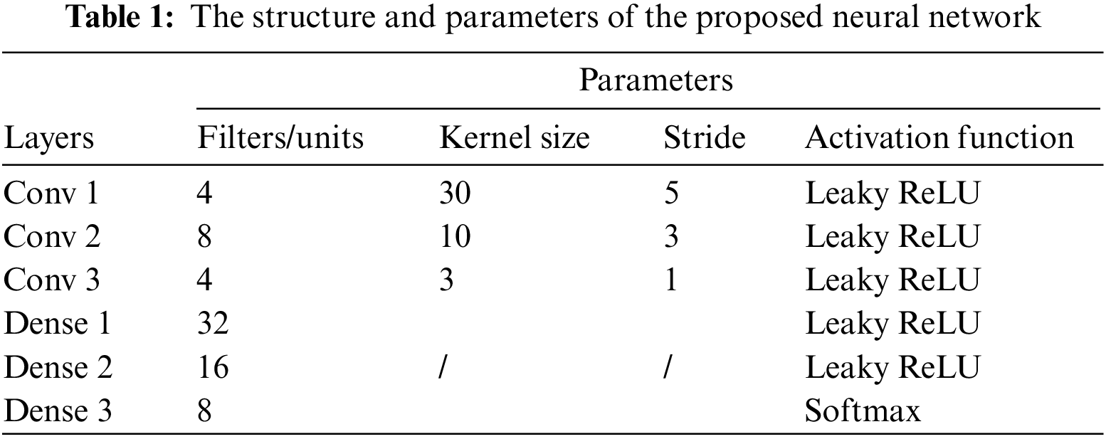
The network for recognizing the wear state of tools discussed in this paper is depicted in Fig. 4. The network is a structure that combines both source and target domain networks, forming a dual-flow system. The source domain network is a supervised classification network that is utilized to carry out the tool wear states classification task based on historical working condition data. The target domain network is an unsupervised network that is utilized to carry out the tool wear states classification task amidst the new operating condition data. The spectrum of the vibration data is a one-dimensional array. 1D convolution is more appropriate for handling 1D data compared to 2D convolution. Thus, the article utilizes 1D convolution to analyze spectral data. The network consists of 1D convolution layers (Conv layer) that share the same domain, as well as domain-shared full connection layers (Dense layer). The source domain network has been trained to obtain the optimal network parameters on the source domain. This training task pertains to the model pre-training discussed in Section 3.5. Table 1 shows the neural network parameters and activation function of each layer. Currently, there is no research that can demonstrate the effectiveness of utilizing more adaptive units in enhancing the model’s performance. The adaptation layer is placed on the penultimate layer, which serves as the transfer of knowledge. The adaptation layer employs the maximum mean difference algorithm to restrict the distribution discrepancy between two parallel networks. The realization of feature alignment between the new and the old working conditions can be achieved.

Figure 4: Tool wear state recognition model

3.4 Model Learning Task

The tool wear state recognition model presented in this paper encompasses two fundamental learning tasks. The first task is the classification of source domains, while the second one involves minimizing distribution discrepancies between domains.

Source domain classification task: g:𝒳→𝒵 represents the feature extractor that is responsible for mapping the sample data to the deep feature vectors. The classifier, represented by f:𝒵→𝒴, is utilized to map the deep feature vectors to prediction labels. Θg is the parameter set of the feature extractor, and Θf is the parameter set of the classifier. The optimization direction of this task is to reduce classification error. The specific optimization goal can be expressed as

minΘgΘf1Nb∑i=1Nb⁡ℒen(f(g(xsi)),ysi),(7)

where xs represents the data of the source domain, ys is the one-hot code of labels, ℒen(⋅,⋅) represents the Categorical Cross Entropy loss function.

Inter-domain distribution discrepancy minimization task: to estimate the inter-domain distribution discrepancy, Eq. (6) can be utilized to generate deep feature vectors that originate from both the source domain and the target domain network adaptation layer. The Eq. (8) defines the task of minimizing the discrepancy between domains in distribution.

minΘgΘfD^ℋ2(g(ℬs),g(ℬt))(8)

3.5 Model Training Method

The model training method of the proposed transfer learning model is as follows, drawing upon the two learning tasks outlined in Section 3.4:

(1) Model pre-training: the labeled data samples from the source domain are utilized to train the source domain network, thus endowing the model with the fundamental capability for source domain classification. Eq. (7) presents the optimization objective. The Mini-batch Stochastic Gradient Descent algorithm is utilized to modify neural network parameters. The Adam optimization algorithm is utilized to fine-tune the learning rate. In the literature, neural networks typically employ normal training methods. As a result, the source domain classification network has good performance on test samples.

(2) Transfer learning training: the aim of transfer learning is to overcome the disparity in distribution between the target and source domains by bridging the gap in the deep feature space. Simultaneously, the capability for classifying source domain data should be maintained. The optimization target is Eq. (9), where α serves as a weight parameter to govern the learning process. The training method for transfer learning is identical to that of pre-training.

minΘgΘf1Nb∑i=1Nb⁡ℒen(f(g(xsi)),ysi)+αD^ℋ2(g(ℬs),g(ℬt))(9)

(3) Tool wear state recognition of target domain data: after model training, the classification network, which is composed of feature extractor and classifier, can be utilized to assess the tool wear state of the target domain’s monitoring data.

4  Experiment and Discussion

4.1 Setup

To verify the performance of the proposed model, a full-life cutting experiment was conducted on milling tools in a 3-axis vertical CNC machine center (FEELER VMC650). A quick-feed milling cutter is utilized in the experiment, which has four inserts. The workpiece material is annealed Cr12MoV die steel. The vibration sensor (PCB 357B03) is employed to gather the cutting vibration of the CNC machine spindle. The machine tool spindle has three mutually perpendicular sensors installed. The data acquisition recorder (NI PXIE-1078) is utilized to store vibration signal data. The sampling frequency is 128,000 Hz. An industrial camera (KEYENCE CV-035 M) is utilized to capture the images of the flanks of four inserts. Fig. 5 displays the experimental platform.

Figure 5: Cutting experimental platform

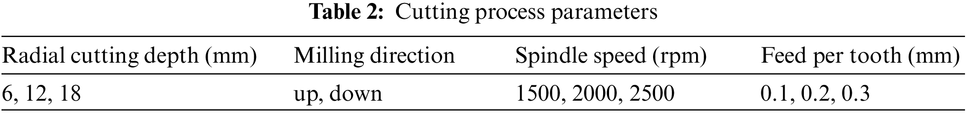
The implementation of this experiment should be relatively straightforward and enable the collection of a substantial amount of high-quality vibration monitoring data. The experiment solely utilizes a single type of tool, workpiece, and material. This paper primarily investigates the transfer of models across various process parameters. Model transfer between different tools and workpieces is not included. The milling task involves multi-parameters plane milling, which is carried out through plane reciprocating cutting. The workpiece plane size is 200 mm * 200 mm. The cutting conditions are set by altering the radial cutting depth, milling direction, spindle speed and feed per tooth. In Table 2, a variety of processing parameters are presented. For every working condition, the cutting area measures 200 mm * 50 mm. The cutting process under each operating condition is completed with a single step. A cutting cycle is completed by performing 54 steps. The cutting process is repeated 65 times throughout the entire life span. During the experimental cutting process, the vibration data is collected continuously and images of the flank are collected after each cycle.

4.2 Monitoring Data Processing

The method outlined in Section 3.2 is utilized to process the monitoring data in order to obtain the training dataset for the model. The threshold of 100 points is selected as the judgment criterion (2 m/s2) to detect the effective cutting stroke and the empty stroke signal segments. To obtain the original cutting vibration signal sample, the effective cutting stroke signal is divided by 1 s. Fig. 6 depicts the cutting vibration signal in the 30th cutting cycle under various operating conditions.

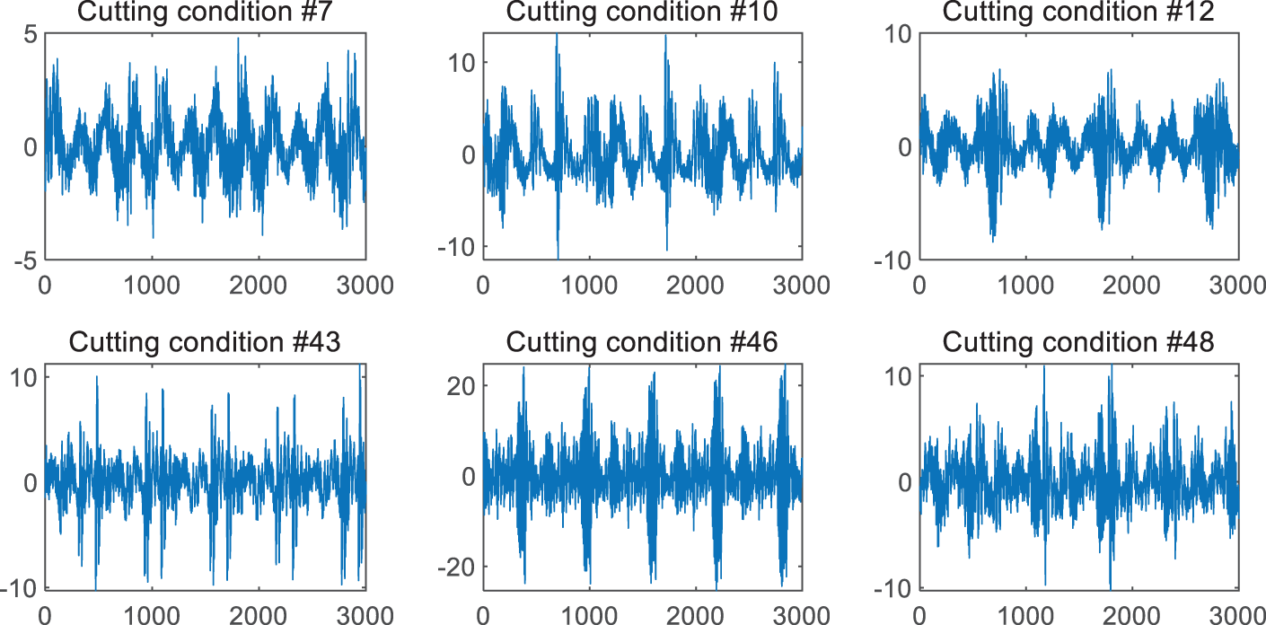
Figure 6: X-axis vibration signal under different cutting conditions

The Fourier transform is applied to the vibration signal sample in order to obtain the spectrum data. The spectrum of varying cutting conditions is depicted in Fig. 7. The figure reveals that the distribution of spectrum data for varying cutting conditions under the same wear state exhibits comparable traits, while the magnitude of the amplitude demonstrates significant differences. The spectrum distribution differs from one cutting condition to another, even though the wear states remain the same. Finally, the spectrum within the sample is normalized. The initial 4000 spectral data points are chosen as the training data for the tool wear recognition model. The band needs to be folded in a specific format, where 2×2000.

Figure 7: X-axis vibration signal spectrum under different cutting conditions

In the present study, the average VB value of four inserts during 65 cutting cycles was determined using the image processing method outlined in Section 3.2. The health status of the tool is determined by analyzing the trend and the value of changes. The cycle scopes for the four wear states are as follows: 1–10, 11–44, 45–54, and 55–65. Fig. 8 displays the average wear value curve of the experimental tool.

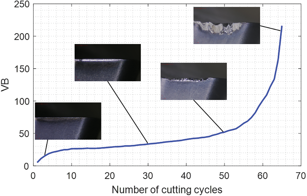
Figure 8: Average wear value curve

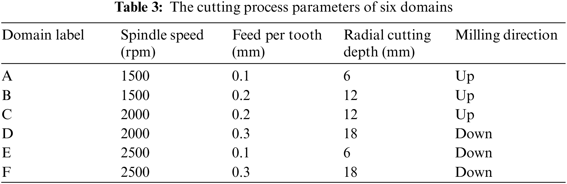
In the present study, six different cutting conditions were chosen to test the tool wear monitoring approach outlined in this paper. The principle behind selecting six working conditions is to maximize the variety of process parameter changes, thereby increasing the complexity of transfer learning. The power and signal-to-noise ratio of vibration signals vary under different operating conditions. However, when subjected to the same wear state with varying cutting conditions, the contact stiffness between the tool and workpiece remains the same, resulting in similar spectral distribution characteristics in their corresponding monitoring samples. Table 3 shows the parameters for six operating conditions. Each cutting condition is a distinct domain. To conduct unsupervised transfer learning of the tool wear state recognition model, a set of working condition data will be designated as the source domain, while another set will be designated as the target domain. The training task is represented as “X→Y”. For instance, A→B denotes a transfer learning task that has source domain A and target domain B.

4.3 Model Performance Analysis

4.3.1 Algorithm Evaluation Index

The performance of the transfer learning algorithm is evaluated using the transfer loss and transfer rate, as depicted in Eqs. (10) and (11), respectively. errt,t indicates the error within a domain. The error occurs when the model is trained on labeled samples from the target domain, and subsequently tested on the same samples. It may be utilized to characterize the difficulty of classification in the target domain. The transfer error is referred to as errs,t. The error is the result of testing the transfer learning model in the target domain. The transfer loss can be used to assess the efficiency of the transfer learning approach. The transfer learning is more effective when the loss value is smaller. To compare the performance of different algorithms in the same task, this paper chooses the source domain classification network in the proposed tool wear state recognition model as the benchmark algorithm to calculate errbt,t. The transfer rate Rtl is utilized to assess the efficiency of models on various tasks. The intra-domain accuracy is used as the denominator, while the transfer accuracy is utilized as the numerator, and the results of various transfer tasks are averaged. The transfer rate Rtl has a positive correlation with the effectiveness of the transfer learning algorithm.

Ltl=errs,t−errbt,t(10)

Rtl=1m∑i=1m⁡[(1−errs,t)/(1−errbt,t)](11)

4.3.2 Task Weight Parameter Optimization

The task of source domain classification and the task of minimizing the distribution discrepancy between domains must be completed simultaneously in order to optimize the tool wear state recognition model in this study. Hyperparameters α are utilized to regulate the model’s optimization direction. The value of this will have an immediate impact on the model’s final performance. In our study, the tasks (A→C, B→E, D→F) was used to optimize the task weight.

When α=0, the relationship between the source domain classification cross entropy (SDCE) and the MMD is shown in Fig. 9. Under this scenario, model training is exclusively carried out for the purpose of source domain classification task. The curve reveals that during the initial phase of training optimization, the SDCE value is significant, whereas the MMD value remains small. The reason for this is that the model employs random initialization. During the process of transmitting forward to deep space, the original samples are blended with random noise, which causes a difference in the distribution of deep features between the source domain and the target domain. As the number of training epochs increases, the model’s ability to match with the source domain classification task improves, while its applicability to the target domain decreases. The disparity in distribution between the target and source domains in the deep feature space is increasing. The training outcome will be that the model is restricted to the source domain data and cannot be applied to the target domain data. This demonstrates that it is imperative to conduct transfer learning for the tool wear recognition model in response to alterations in the working condition.

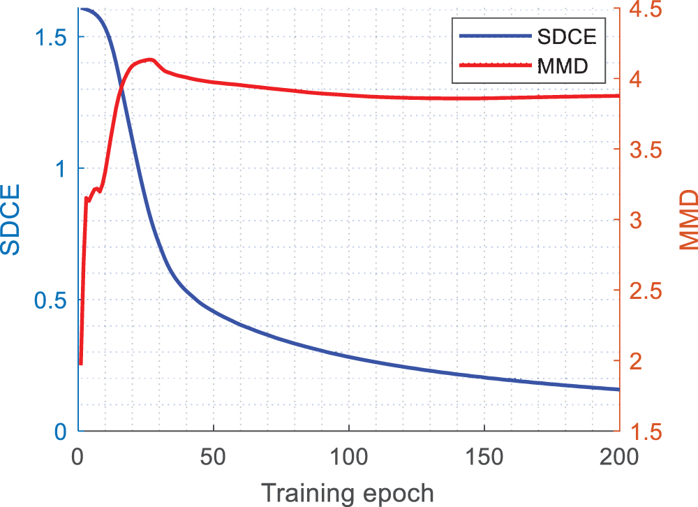
Figure 9: The training process of the proposed model when α=0

The significance of α can impact the training model’s optimization direction, ultimately determining its performance in both the target and source domains. Therefore, this study needs to optimize the value of α. We conducted the model training on three tasks for each α. The mean value of MMD for the trained models on the test set, as well as its classification accuracy on the target domain test set, were both recorded. Fig. 10 illustrates the correlation between the mean value of MMD and α. When comparing Figs. 9 and 10, it is evident that MMD holds a significant position in model optimization. When α=0.3, the MMD value is 1.4, which is nearly 3 times less than the value when α=0. As the value of α increases, the adaptability of the deep feature space domain is strengthened, causing a gradual decrease in the MMD value.

Figure 10: The correlation between the MMD and the task weight

In Fig. 11, the classification accuracy of the model on the test set of target domain is depicted as α varies. It is evident that any α can enhance the model’s classification accuracy in the target domain. The accuracy of classification, however, initially surges and ultimately declines as the value progresses. This indicates that an excessively high value of α will cause the deep features to clump together, leading to heightened classification complexity and diminished classification precision. The highest model classification accuracy of 86% was achieved when α=0.3.

Figure 11: The correlation between the classification accuracy and the task weight

4.3.3 Model Performance Analysis

In order to confirm the effectiveness of the proposed dual-flow model with a domain-adaptive layer (DFMDA), five transfer learning tasks were developed by utilizing the domains presented in Table 3 to identify the tool wear state across different cutting conditions. The weight parameter α was set as 0.3. In order to explain the advantages of the model in this paper, this section reproduces the methods disclosed in several documents, such as adversarial domain adaptation transfer learning model (ADATLM) [39], and pretrained transfer learning model (PTLM) [40].

Fig. 12 displays the models’ performance on six learning tasks, and the accuracy are achieved in the target domain test set. The baseline model 1DCNN, which does not utilize transfer learning, achieves a classification accuracy of only 55%. It holds no practical significance. On the other hand, three transfer learning methods considerably enhance the accuracy of target domain testing. The transfer learning tasks of the method proposed in this paper have achieved the highest test accuracy, with an accuracy rate of over 80% in the other two transfer learning tasks. This demonstrates that the method proposed in this paper outperforms the other two methods.

Figure 12: Model performance comparison on six learning tasks

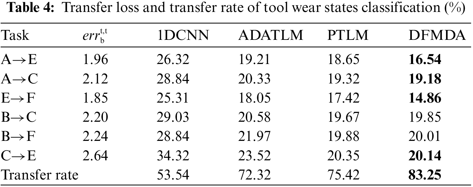
Table 4 displays the transfer loss and transfer rate of diverse models in each task. Our proposed model obtains the lowest transfer loss across four tasks. The transfer rate of up to 83.25% as a multi-task statistical indicator further validates the robustness of the proposed method.

5  Conclusion

The severe wear of metal tools has an impact on the quality of cutting. To improve the quality of the workpiece, it is essential to monitor the health states of the tool. This paper proposes a tool wear states recognition model based on unsupervised transfer learning for multi-condition cutting environments. The model’s structure is simple and comprises a convolutional neural network and a multilayer perceptron network. The recognition model is trained using labeled source domain and unlabeled target domain data, allowing for the implementation of both classification and deep feature distribution adaptation tasks. The experimental results presented in our study demonstrate that the proposed model outperforms the methods currently available in the target domain.

In the subsequent phase of research, the study may delve deeper into transfer learning in intricate situations where a variety of tools and workpieces, including CNC machines, are involved. The method of distributing data should be improved. In future research, the transfer learning of multiple source domains could be taken into account to enhance the robustness and applicability of deep learning models.

Acknowledgement: The authors want to thank the editor and reviewers for valuable comments.

Funding Statement: This work is supported by the National Key Research and Development Program of China (No. 2020YFB1713500); the Natural Science Basic Research Program of Shaanxi (Grant No. 2023JCYB289) and the National Natural Science Foundation of China (Grant No. 52175112) and the Fundamental Research Funds for the Central Universities (Grant No. ZYTS23102).

Author Contributions: The authors confirm contribution to the paper as follows: study conception and design: Qixin Lan, Binqiang Chen, Yao Bin, Wangpeng He; data collection: Qixin Lan; analysis and interpretation of results: Binqiang Chen, Qixin Lan, Yao Bin; draft manuscript preparation: Qixin Lan. All authors reviewed the results and approved the final version of the manuscript.

Availability of Data and Materials: Readers can contact us via the corresponding author’s email address to inquire about the acquisition method of the data in this article. Due to intellectual property protection, we cannot provide raw data, only processed data.

Conflicts of Interest: The authors declare that they have no conflicts of interest to report regarding the present study.

References

1. Stavropoulos, P., Papacharalampopoulos, A., Vasiliadis, E., Chryssolouris, G. (2016). Tool wear predictability estimation in milling based on multi-sensorial data. International Journal of Advanced Manufacturing Technology, 82, 509–521. [Google Scholar]

2. Liao, X. P., Zhou, G., Zhang, Z. K., Lu, J., Ma, J. Y. (2019). Tool wear state recognition based on GWO-SVM with feature selection of genetic algorithm. International Journal of Advanced Manufacturing Technology, 104, 1051–1063. [Google Scholar]

3. Chen, N., Hao, B. J., Guo, Y. L., Li, L., Khan, M. A. et al. (2020). Research on tool wear monitoring in drilling process based on APSO-LS-SVM approach. International Journal of Advanced Manufacturing Technology, 108, 2091–2101. [Google Scholar]

4. Li, X. B., Liu, X. L., Yue, C. X., Liu, S. Y., Zhang, B. W. et al. (2021). A data-driven approach for tool wear recognition and quantitative prediction based on radar map feature fusion. Measurement, 185, 110072. [Google Scholar]

5. Bazi, R., Benkedjouh, T., Habbouche, H., Rechak, S., Zerhouni, N. (2022). A hybrid CNN-BiLSTM approach-based variational mode decomposition for tool wear monitoring. International Journal of Advanced Manufacturing Technology, 119, 3803–3817. [Google Scholar]

6. Zhang, C., Zhang, J. L. (2013). On-line tool wear measurement for ball-end milling cutter based on machine vision. Computers in Industry, 64, 708–719. [Google Scholar]

7. Qin, A. P., Guo, L., You, Z. C., Gao, H. L., Wu, X. D. et al. (2020). Research on automatic monitoring method of face milling cutter wear based on dynamic image sequence. International Journal of Advanced Manufacturing Technology, 110, 3365–3376. [Google Scholar]

8. Zhou, J. H., Pang, C. K., Zhong, Z. W., Lewis, F. L. (2011). Tool wear monitoring using acoustic emissions by dominant-feature identification. IEEE Transactions on Instrumentation and Measurement, 60, 547–559. [Google Scholar]

9. Duspara, M., Sabo, K., Stoic, A. (2014). Acoustic emission as tool wear monitoring. Tehnicki Vjesnik-Technical Gazette, 21, 1097–1101. [Google Scholar]

10. Ou, J. Y., Li, H. K., Huang, G. J., Liu, B., Wang, Z. D. (2021). Tool wear recognition based on deep kernel autoencoder with multichannel signals fusion. IEEE Transactions on Instrumentation and Measurement, 70, 1–9. [Google Scholar]

11. Akbari, A., Danesh, M., Khalili, K. (2017). A method based on spindle motor current harmonic distortion measurements for tool wear monitoring. Journal of the Brazilian Society of Mechanical Sciences and Engineering, 39, 5049–5055. [Google Scholar]

12. Kilundu, B., Dehombreux, P., Chiementin, X. (2011). Tool wear monitoring by machine learning techniques and singular spectrum analysis. Mechanical Systems and Signal Processing, 25, 400–415. [Google Scholar]

13. Stavropoulos, P., Papacharalampopoulos, A., Souflas, T. (2020). Indirect online tool wear monitoring and model-based identification of process-related signal. Advances in Mechanical Engineering, 12, 1–12. [Google Scholar]

14. Liu, B., Li, H. K., Ou, J. Y., Wang, Z. D., Sun, W. (2022). Intelligent recognition of milling tool wear status based on variational auto-encoder and extreme learning machine. International Journal of Advanced Manufacturing Technology, 119, 4109–4123. [Google Scholar]

15. da Silva, R. H. L., da Silva, M. B., Hassui, A. (2016). A probabilistic neural network applied in monitoring tool wear in the end milling operation via acoustic emission and cutting power signals. Machining Science and Technology, 20, 386–405. [Google Scholar]

16. Ai, C. S., Sun, Y. J., He, G. W., Ze, X. B., Li, W. et al. (2012). The milling tool wear monitoring using the acoustic spectrum. International Journal of Advanced Manufacturing Technology, 61, 457–463. [Google Scholar]

17. Nguyen, V., Nguyen, V., Pham, V. (2020). Deep stacked auto-encoder network based tool wear monitoring in the face milling process. Journal of Mechanical Engineering/Strojniški Vestnik, 66, 227–234. [Google Scholar]

18. Tangjitsitcharoen, S., Lohasiriwat, H. (2018). Intelligent monitoring and prediction of tool wear in CNC turning by utilizing wavelet transform. International Journal of Advanced Manufacturing Technology, 99, 2219–2230. [Google Scholar]

19. Hou, W., Zhang, C., Jiang, Y., Cai, K., Wang, Y. et al. (2023). A new bearing fault diagnosis method via simulation data driving transfer learning without target fault data. Measurement, 215, 112879. [Google Scholar]

20. Xie, Y., Zhang, C. Y., Liu, Q. (2021). Tool wear status recognition and prediction model of milling cutter based on deep learning. IEEE Access, 9, 1616–1625. [Google Scholar]

21. Azmi, A. I., Lin, R. J. T., Bhattacharyya, D. (2013). Tool wear prediction models during end milling of glass fibre-reinforced polymer composites. International Journal of Advanced Manufacturing Technology, 67, 701–718. [Google Scholar]

22. Zhang, X. D., Han, C., Luo, M., Zhang, D. H. (2020). Tool wear monitoring for complex part milling based on deep learning. Applied Sciences, 10, 6916. [Google Scholar]

23. Qin, Y. R., Li, J. F., Zhang, C. X., Zhao, Q. P., Ma, X. F. (2022). A dual-stage attention model for tool wear prediction in dry milling operation. Entropy, 24, 1733. [Google Scholar] [PubMed]

24. Shah, M., Vakharia, V., Chaudhari, R., Vora, J., Pimenov, D. Y. et al. (2022). Tool wear prediction in face milling of stainless steel using singular generative adversarial network and LSTM deep learning models. International Journal of Advanced Manufacturing Technology, 121, 723–736. [Google Scholar]

25. Li, Z. M., Zhong, W., Shi, Y. G., Yu, M., Zhao, J. et al. (2022). Unsupervised tool wear monitoring in the corner milling of a titanium alloy based on a cutting condition-independent method. Machines, 10, 616. [Google Scholar]

26. Pan, T. H., Zhang, J., Zhang, X., Zhao, W. H., Zhang, H. J. et al. (2022). Milling force coefficients-based tool wear monitoring for variable parameter milling. International Journal of Advanced Manufacturing Technology, 120, 4565–4580. [Google Scholar]

27. Pan, S. J., Yang, Q. A. (2010). A survey on transfer learning. IEEE Transactions on Knowledge and Data Engineering, 22, 1345–1359. [Google Scholar]

28. Feuz, K. D., Cook, D. J. (2015). Transfer learning across feature-rich heterogeneous feature spaces via feature-space remapping (FSR). ACM Transactions on Intelligent Systems and Technology, 6, 1–27. [Google Scholar]

29. Jiang, S. Y., Xu, Y. H., Wang, T. Y., Yang, H. Z., Qiu, S. J. et al. (2019). Multi-label metric transfer learning jointly considering instance space and label space distribution divergence. IEEE Access, 7, 10362–10373. [Google Scholar]

30. Lee, K., Han, S., Pham, V. H., Cho, S., Choi, H. J. et al. (2021). Multi-objective instance weighting-based deep transfer learning network for intelligent fault diagnosis. Applied Sciences, 11, 2370. [Google Scholar]

31. Liao, Y. X., Huang, R. Y., Li, J. P., Chen, Z. Y., Li, W. H. (2021). Dynamic distribution adaptation based transfer network for cross domain bearing fault diagnosis. Chinese Journal of Mechanical Engineering, 34, 1–10. [Google Scholar]

32. Li, J. B., Lu, J., Chen, C. Y., Ma, J. Y., Liao, X. P. (2021). Tool wear state prediction based on feature-based transfer learning. International Journal of Advanced Manufacturing Technology, 113, 3283–3301. [Google Scholar]

33. Kaya, M., Bilge, H. S. (2019). Deep metric learning: A survey. Symmetry, 11, 1066. [Google Scholar]

34. Tzeng, E., Hoffman, J., Saenko, K., Darrell, T. (2017). Adversarial discriminative domain adaptation. 30th IEEE Conference on Computer Vision and Pattern Recognition (CVPR 2017), pp. 2962–2971. Honolulu, HI, USA, IEEE. [Google Scholar]

35. Ganin, Y., Lempitsky, V. (2015). Unsupervised domain adaptation by backpropagation. International Conference on Machine Learning, vol. 37, pp. 1180–1189. Lille, France, JMLR. [Google Scholar]

36. Tan, C. Q., Sun, F. C., Kong, T., Zhang, W. C., Yang, C. et al. (2018). A survey on deep transfer learning. In: Artificial neural networks and machine learning—ICANN 2018, pp. 270–279. Cham: Springer. [Google Scholar]

37. Borgwardt, K. M., Gretton, A., Rasch, M. J., Kriegel, H. P., Scholkopf, B. et al. (2006). Integrating structured biological data by kernel maximum mean discrepancy. Bioinformatics, 22, E49–E57. [Google Scholar] [PubMed]

38. Gretton, A., Borgwardt, K. M., Rasch, M. J., Scholkopf, B., Smola, A. (2012). A kernel Two-sample test. Journal of Machine Learning Research, 13, 723–773. [Google Scholar]

39. Li, K., Chen, M. S., Lin, Y. C., Li, Z., Jia, X. S. et al. (2022). A novel adversarial domain adaptation transfer learning method for tool wear state prediction. Knowledge-Based Systems, 254, 109537. [Google Scholar]

40. Bahador, A., Du, C. L., Ng, H. P., Dzulqarnain, N. A., Ho, C. L. (2022). Cost-effective classification of tool wear with transfer learning based on tool vibration for hard turning processes. Measurement, 201, 111701. [Google Scholar]