Computational Analysis of Novel Extended Lindley Progressively Censored Data

Abbreviations

1  Introduction

One of the key research areas in the concept of distribution theory is the evolution of suggesting new statistical distributions. Such generalized distributions allow modelling for a range of disciplines, including reliability, engineering and medicine with even greater flexibility. The two-parameter Marshall-Olkin-Lindley (MOL) distribution suggested by Ghitany et al. [1] is one of the novel versions of Marshall-Olkin models that take the conventional Lindley distribution as a baseline distribution. Assume that X is a lifetime random variable of an experimental item that follows the MOL distribution, denoted by MOL(θ,σ), with shape parameter θ and scale parameter σ.

Hence, its probability density function (PDF), g(⋅), reliability function (RF), R(⋅), and hazard rate function (HRF), h(⋅), of x>0, are given, respectively, by:

g(x;θ,σ)=θσ2e−σx(x+1)(σ+1)[1−θ¯e−σx(1+σxσ+1)]2, θ,σ>0,(1)

R(x;θ,σ)=θe−σx(1+σxσ+1)1−θ¯e−σx(1+σxσ+1)(2)

and

h(x;θ,σ)=σ2(x+1)[σ(x+1)+1][1−θ¯e−σx(1+σxσ+1)],(3)

where θ¯=1−θ. Obviously, the Lindley distribution can be obtained from (1) as a special case by setting θ=1. Using some specified values on the MOL’s parameters of θ and σ, via R 4.1.2 software, we plotted various shapes of the PDF and HRF of the MOL distribution, see Fig. 1. It shows that the density shapes are unimodal or decreasing while the HRF shapes are increasing, bathtub and unimodal then bathtub. Since these hazard rate shapes are quite beneficial in lifetime data modelling, hence the MOL distribution is justly flexible and can be considered to provide a good description of different plans of censored data, for details see Ghitany et al. [1]. A look at the literature reveals that just one study by do Espirito Santo et al. [2] used a complete sample to explore the estimations of the MOL distribution using six classical estimation approaches. On the other hand, no study considered the MOL distribution in the censoring case.

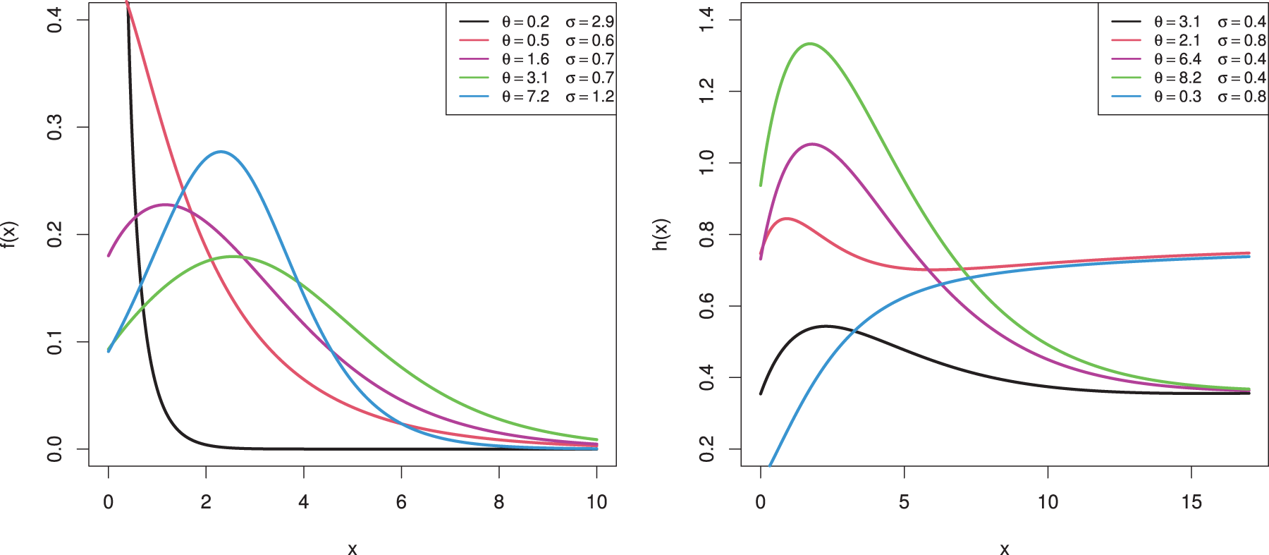
Figure 1: Various shapes for the density and hazard functions of MOEL distribution

Frequently, life testing studies are stopped before all of the components fail. Due to financial or time restrictions, it occurs. The observations that emerge from this type of scenario are known as the censored sample. The literature has developed a number of filtering techniques for the evaluation of various life-testing strategies. The two most popular censorship techniques among the various techniques are Types I and II. The experimental units cannot be removed during a life-testing experiment, however, under any of these censorship techniques. This adaptability is featured in a life-testing experiment with progressive censoring. Since the publication of the book by Balakrishnan et al. [3], extensive research has been conducted on the various facets of progressive censoring. A recent book by Balakrishnan et al. [4] has an extensive compilation of different studies connected to the progressive censorship strategy.

In order to estimate the parameters of the MOL distribution, we work with the progressive Type-II censored (PT-IIC) sample in this study. The PT-IIC sample can be explained as follows: assume that a life testing experiment involving n units with a predetermined number progressive censoring scheme R=(R1,R2,…,Rm), where m<n is the desired number of observed failures. At the time of the first failure X1:m:n, the experiment is stopped and R1 working units are removed. The experiment then resumes using the remaining n−1−R1 units, and when it reaches the second failure, X2:m:n, it is stopped and R2 operating units are removed at random from the remaining n−2−R1 units, and so on. The experiment ends and all of the remaining units n−m−∑i=1m−1Ri are eliminated when it reaches the mth failure time Xm:m:n. The ordered observed failure times in this case are given by X1:m:n<X2:m:n<⋯<Xm:m:n, and the likelihood function for a PT-IIC sample can be expressed as:

L=A∏i=1mg(xi:m:n)[1−G(xi:m:n)]Ri,(4)

where A is a constant that is independent of the parameters and G(x)=1−R(x). For several practical lifetime models, a number of inferential techniques based on the PT-IIC scheme have been introduced. For instance, see Sultan et al. [5], Guo et al. [6], Joukar et al. [7], Elshahhat et al. [8], Alotaibi et al. [9], Okasha et al. [10] and Maiti et al. [11], as well as the references therein.

Due to the MOL distribution’s flexibility and the PT-IIC scheme’s effectiveness in gathering sample data, no study investigated the estimation problems of the MOL distribution in the case of the PT-IIC sample. Also, in the original work of Ghitany et al. [1], they just used the maximum likelihood approach to estimate the parameters of the MOL distribution without saying anything about the Bayesian estimation method. In addition, they estimated only the unknown parameters, while it is of interest to reliability engineers and other practitioners to see the performance of the reliability measures of the used distribution. Therefore, this paper’s main goal is to examine frequentist and Bayesian inferences of the MOL distribution’s unknown parameters under the PT-IIC, along with the related reliability indices, such as the RF and HRF. As expected, it is found that the maximum likelihood estimators (MLEs) of θ and σ cannot be derived in closed form; instead, they must be obtained by simultaneously solving two non-linear equations. The MLEs of the RF and HRF are obtained using the invariance property. We suggest constructing the approximative confidence intervals (ACIs) for the various parameters, including RF and HRF, using the asymptotic distribution of the MLEs. We also take into account the Bayesian inference based on independent gamma priors and use two loss functions: squared error (SE) and general entropy (GEnt), which serve as symmetric and asymmetric loss functions, respectively. Due to the fact that the Bayesian estimators cannot be derived in closed form, we suggest using the Markov Chain Monte Carlo approach to get point estimates and the highest posterior density (HPD) credible intervals. The overall performance of the various techniques is compared using Monte Carlo simulations, and two data sets with various progressive censoring plans are examined for illustration.

The remainder of the article is structured as follows. We present the MLEs and ACIs of the unknown parameters, RF and HRF, in Section 2. We acquire the Bayesian inference in Section 3. Sections 4 and 5 separately describe the findings of the Monte Carlo simulation and the analysis of two data sets, respectively. At last, we sum up the paper in Section 6.

2  Maximum Likelihood Estimation

In this part, we estimate the unknown parameters, RF and HRF of the MOL distribution using the method of maximum likelihood based on the PT-IIC sample. The ACIs of the different parameters are explained in addition to the point estimators. Assume that x1:m:n,x2:m:n,...,xm:m:n is a PT-IIC sample of size m with progressive pattern R1,…,Rm taken from the MOL population with PDF and RF as displayed in (1) and (2), respectively. Then the likelihood function, without the constant term, takes the following form based on (1) and (2), and (4):

L(θ,σ)=θnσ2m(σ+1)me−σ∑i=1m(1+Ri)xi∏i=1m(1+σyi)Ri[1+σ−θ¯e−σxi(1+σyi)]2+Ri,(5)

where xi=xi:m:n for simplicity and yi=1+xi. The log-likelihood function is expressed as follows, using Eq. (5):

ℓ(θ,σ)=nlog⁡(θ)+2mlog⁡(σ)+mlog⁡(σ¯)−σ∑i=1m(1+Ri)xi+∑i=1mRilog⁡(1+σyi)−∑i=1m(2+Ri)log⁡[σ¯−θ¯e−σxi(1+σyi)],(6)

where σ¯=σ+1. The likelihood equations are derived by calculating the first partial derivatives of (6) with regard to θ and σ and equating each one to zero as shown below:

∂ℓ(θ,σ)∂θ=nθ−∑i=1m(2+Ri)e−σxi(1+σyi)σ¯−θ¯e−σxi(1+σyi)=0(7)

and

∂ℓ(θ,σ)∂σ=2mσ+mσ¯−∑i=1m(1+Ri)xi+∑i=1mRiyi1+σyi−∑i=1m(2+Ri)ψiσ¯−θ¯e−σxi(1+σyi)=0,(8)

where ψi=1−θ¯e−σxi[yi−xi(1+σyi)]. It is obvious that analytical solutions to the likelihood equations in (7) and (8) in order to obtain the MLEs of θ and σ, denoted by θ^ and σ^, are not possible. Therefore, to obtain the needed MLEs, any iteration process may be used, including the Newton-Raphson procedure. The MLEs of RF and HRF at a given time t can then be calculated using the invariance property of MLEs once the MLEs θ^ and σ^ have been obtained. The MLEs of G(t) and h(t) in this instance are derived from (2) and (3) as follows:

R^(t)=θ^e−σ^t(1+σ^tσ^+1)1−θ¯^e−σ^t(1+σ^tσ^+1)

and

h^(t)=σ^2(t+1)[σ^(t+1)+1][1−θ¯^e−σ^t(1+σ^tσ^+1)].

Utilizing the asymptotic normality of the MLEs is the most common approach for establishing confidence bounds for the parameters. The MLEs’ asymptotic distribution can be expressed as (θ^,σ^)∼N[(θ,σ),J−1(θ,σ)], where J−1(θ,σ) stands for the variance-covariance matrix obtained based on the Fisher information matrix denoted by J. In practice, we use J−1(θ^,σ^) to estimate J−1(θ,σ) due to the challenging second derivative expressions. In this case, we can write J−1(θ^,σ^) as follows:

J−1(θ^,σ^)=(−∂2ℓ(θ,σ)∂θ2−∂2ℓ(θ,σ)∂θ∂σ−∂2ℓ(θ,σ)∂σ∂θ−∂2ℓ(θ,σ)∂σ2)(θ,σ)=(θ^,σ^)−1=(var^(θ^)cov^(θ^,σ^)cov^(σ^,θ^)var^(σ^)),(9)

with

∂2ℓ(θ,σ)∂θ2=−nθ2−∑i=1m(2+Ri)e−2σxi(1+σyi)2ϕi2,

∂2ℓ(θ,σ)∂σ2=−2mσ2−mσ¯2^+∑i=1mRiyi2(1+σyi)2−∑i=1m(2+Ri)ϖiϕi−∑i=1m(2+Ri)ψi2ϕi2

and

∂2ℓ(θ,σ)∂θ∂σ=∑i=1m(2+Ri)ψ´iϕi−∑i=1m(2+Ri)e−σxi(1+σyi)ψiϕi2,

where ϕi=σ¯−θ¯e−σxi(1+σyi) and ϖi=xiθ¯e−σxi[xi(1+σyi)−2yi] and ψ´i=e−σxi[yi−xi(1+σyi)]. Then, the 100(1−α)% ACIs of θ and σ can be computed, respectively, as:

θ^±zα/2var^(θ^),andσ^±zα/2var^(σ^),

where var^(θ^) and var^(σ^) are the main diagonal elements of (9), respectively, and zα/2 is the upper (α/2)th percentile point of the standard normal distribution. On the other hand, we must first determine the variances of respective estimators for the RF and HRF in order to construct such intervals. Here, we approximate these variances using the delta approach. The following derivatives obtained from (2) and (3), respectively, are required in order to use the delta method:

Rθ=∂R(t;θ,σ)∂θ=G(t;θ,σ)θ[1−R(t;θ,σ)],

Rσ=∂R(t;θ,σ)∂σ=θte−σtσ¯ϕt−θ¯tσR(t;θ,σ)e−σt(1+σ¯yt)σ¯2ϕt−tR(t;θ,σ),

hθ=∂h(t;θ,σ)∂θ=−h(t;θ,σ)e−σt(1+σyt)ϕtσ¯

and

hσ=∂h(t;θ,σ)∂σ=σytϕt(1+σyt)[2−σyt(1+σyt)]−θ¯tσh(t;θ,σ)e−σt(1+σ¯yt)σ¯2ϕt,

where ϕt=σ¯−θ¯e−σt(1+σ(1+t)) and yt=1+t.

Suppose that ΔR=(Rθ,Rσ)|(θ,σ)=(θ^,σ^) and Δh=(hθ,hσ)|(θ,σ)=(θ^,σ^), then we can obtain the approximated estimated variances of R^(t) and h^(t), respectively, as follows:

var^(R^)≈[ΔRJ−1(θ^,σ^)ΔR⊤]andvar^(h^)≈[ΔhJ−1(θ^,σ^)Δh⊤],

As a result, with 100(1−α)% confidence level, the ACIs that align to G(t) and h(t) can be acquired, respectively, as follows:

R^(t)±zα/2var^(R^),andh^(t)±zα/2var^(h^).

3  Bayesian Estimation

For analyzing failure time data, the Bayesian estimation approach has attracted a lot of attention. It uses one’s past knowledge of the parameters and also takes into account the information that is readily available. In this section, the Bayesian estimators of θ,σ,R(t) and h(t) are considered under the assumption that the two unknown parameters are independent and have gamma prior distributions. We consider the use of independent gamma priors due to the flexibility of gamma distribution and to avoid adding more complexity to the posterior distribution. Moreover, independent priors are considered because they are rather straightforward and concise, which may not produce many challenging computational and inferential problems. Despite dependent priors appearing more appealing in some practical contexts, the dependent property between parameters cannot be justified subjectively based on historical data and expert knowledge where such prior information may be extremely rare. Hence, for the sake of simplicity, independent priors are more widely used in statistics under the Bayesian method. In order to get the Bayesian estimators, two loss functions are offered to get the point estimators, namely SE and GEnt loss functions. Besides acquiring the point estimators, the HPD credible intervals are also obtained. Suppose that θ∼G(a1,b1) and σ∼G(a2,b2), where aj,bj,j=1,2 are the hyper-parameters. Therefore, the joint prior of θ and σ can be expressed as shown below:

q(θ,σ)∝θa1−1σa2−1e−(b1θ+b2σ),θ,σ>0.(10)

The posterior distribution of the unknown parameters θ and σ can be obtained by combining the likelihood function in (5) with the joint prior distribution provided (10) and by applying the Bayes theorem as follows:

g(θ,σ|x_)=θn+a1−1σ2m+a2−1σ¯me−σ[∑i=1m(1+Ri)xi+b2]−b1θC∏i=1m(1+σyi)Ri[σ¯−θ¯e−σxi(1+σyi)]2+Ri,(11)

where x_=(x1,…,xm) and C is the normalized constant.

If one setting aj=bj=0 for j=1,2 in (10), the joint posterior density (11) will then be in proportion to the likelihood function (5), i.e., g(θ,σ|x_)∝(θσ)−1L(θ,σ), which is the non-informative case. From a Bayesian viewpoint, there is clearly no way in which one can say that one prior is better than any other. Generally, if the proper prior information is available, it is better to use the informative prior(s) than the non-informative prior(s). Otherwise, if one does not have sufficient prior information, it is better to use a non-informative prior distribution. Since the Bayesian estimates using SE loss function with non-informative priors behave like the maximum likelihood estimates whereas those with informative priors behave much better than others, it is always better to use the frequentist estimates rather than the Bayesian estimates because the latter are computationally more expensive when the MCMC procedure is used. In Section 4, to evaluate the sensitivity of the priors, some discussions about various sets of prior distributions are reported.

Now, in order to derive the Bayesian estimators, we take into account the SE and GEnt loss functions. The Bayesian estimator for the SE loss function is the posterior mean, which considers overestimation and underestimation equally. In contrast hand, the GEnt loss function offers different influences for overestimation and underestimation. Calabria et al. [12] introduced the GEnt loss function, which is defined as:

GEnt(λ~,λ)∝(λ~λ)μ−μlog⁡(λ~λ)−1,

where μ is a parameter that controls the level of asymmetry and λ~ is the Bayesian estimator of λ. Below is the Bayesian estimator of λ using the GEnt loss function:

λ~GEnt=[Eλ(λ−μ)]−1μ,(12)

given that Eδ(δ−κ) exists and is finite. Assume that ϑ(θ,σ) is a function of the unknown parameters, we may easily derive its Bayesian estimator using SE and GEnt loss functions, respectively, as follows:

ϑ~SE(θ,σ)=∫0∞∫0∞ϑ(θ,σ)g(θ,σ|x_)dθdσ(13)

and

ϑ~GEnt(θ,σ)=[∫0∞∫0∞[ϑ(θ,σ)]−μg(θ,σ|x_)dθdσ]−1μ(14)

It is obvious that it is difficult to determine the Bayesian estimators using (13) and (14) analytically. In order to acquire the Bayesian estimates of θ and σ and the related HPD credible intervals, we suggest using the MCMC procedure. We must first determine the full conditional distributions of the unknown parameters from (11) as follows:

g(θ|σ,x_)∝θn+a1−1exp⁡{−∑i=1m(2+Ri)log⁡[σ¯−θ¯e−σxi(1+σyi)]−b1θ}(15)

and

g(σ|θ,x_)∝σ2m+a2−1σ¯me−σ[∑i=1m(1+Ri)xi+b2]∏i=1m(1+σyi)Ri[σ¯−θ¯e−σxi(1+σyi)]2+Ri.(16)

It is evident that the conditional distributions of θ and σ as provided in (15) and (16) cannot be represented in standard forms, but their graphs are equivalent to the normal distribution. As a result, we employ the Metropolis-Hastings (M-H) algorithm with normal proposal distribution with asymptotic variances to produce random samples from these distributions. The steps that follow now demonstrate how to get the required samples.

Step 1. Set k=1.

Step 2. Begin with the initial guesses (θ(0),σ(0))=(θ^,σ^).

Step 3. From (15), generate θ(k) using normal proposal distribution, i.e., N(θ(0),var^(θ(0))), by using the M-H steps, where var^(θ(0))≅var^(θ^) is given by (9).

Step 4. Use (16) to get σ(k) using the M-H steps with normal proposal distribution, i.e., N(σ(0),var^(σ(0))), where var^(σ(0))≅var^(σ^) is given by (9).

Step 5. Based on the generated θ(k) and σ(k), obtain

R(k)(t)=θ(k)e−σ(k)t(1+σ(k)tσ(k)+1)1−θ¯(k)e−σ(k)t(1+σ(k)tσ(k)+1)

and

h(k)(t)=σ2(k)(t+1)[σ(k)(t+1)+1][1−θ¯(k)e−σ(k)t(1+σ(k)tσ(k)+1)],

Step 6. Put k=k+1.

Step 7. Repeat steps 3–6, M times to compute

[β(1),…,β(M)],

where β=θ,σ,R(t) or h(t).

In this study, the first B generated samples are discarded in order to ensure convergence and remove the appeal of initial guesses. In this situation, we possess β(k),k=B+1,…,M. The Bayesian estimate of β based on the SE and GEnt loss functions can be calculated using large M, respectively, as:

β~SE=1M−B∑k=B+1Mβ(k)andβ~GEnt={1M−B∑k=B+1M[β(k)]−μ}−1μ.

To construct the HPD credible intervals of β, order β(k),k=B+1,…,M. Therefore, the 100(1−α)% HPD credible interval of β will be [β(k∗),β(k∗+(1−α)(M−B))], where k∗=B+1,B+2,…,M is determined such that:

β(k∗+[(1−α)(M−B)])−β(k∗)=min1⩽l⩽α(M−B)⁡[β(l+[(1−α)(M−B)])−β(k))],

where [ν] stands for the biggest integer that is less than or equal to ν.

4  Monte Carlo Simulation

To evaluate the behavior of the proposed estimators of θ, σ, R(t) and h(t) developed in the proceeding sections, Monte Carlo simulation experiments are conducted. For this target, we simulate 1,000 PT-IIC samples from MOL(0.8,0.4) based on various choices of n, m and progressive pattern R. Taking t=0.2, the actual values of R(t) and h(t) are 0.970 and 0.104, respectively. Using n(=50,90), the proposed numerical experiments are performed by taking m as a failure percentage (FP) of each n as mn(=40, 80)%. Moreover, for each set of (n,m), different progressive patterns R=(R1,R2,…,Rm) are considered as:

Scheme-1: R=(n−m,0∗(m−1)),Scheme-2: R=(0∗(m2−1),n−m,0∗(m2)),Scheme-3: R=(0∗(m−1),n−m),

where R=(1,0,0,0,1) is denoted by R=(1,0∗3,1) for short notation.

Once the 1,000 PT-IIC samples collected, the maximum likelihood and 95% ACI estimates of θ, σ, R(t) and h(t) are calculated utilizing via ’maxLik’ package (by Henningsen et al. [13]) in R 4.1.2 software. To develop the Bayesian MCMC inferences of the same unknown MOL parameters, by according to the mean and variance of the gamma density, two informative sets of the hyperparameters ai and bi for i=1,2 of θ and σ are used namely: prior-1: (a1,a2,b1,b2)=(4,2,5,5) and prior-2: (a1,a2,b1,b2)=(8,4,10,10). Following Kundu [14] and Dey et al. [15], the given hyperparameter values of ai,bi, i=1,2 of the unknown MOL parameters are chosen in such a way that the prior mean becomes the expected value of the corresponding parameter. Using the M-H algorithm sampler, from SE and GEnt (for μ(=−2,+2)) loss functions, the Bayesian point estimates of θ, σ, R(t) and h(t) are calculated based on 12,000 MCMC samples after ignoring the first 2,000 variates as burn-in. Further, from 10,000 MCMC samples, the 95% HPD credible intervals of θ, σ, R(t) or h(t) are calculated also. All Bayesian evaluations of the unknown parameters θ and σ or the reliability time parameters R(t) and h(t) are performed via ’coda’ package (by Plummer et al. [16]) in R 4.1.2 software. All necessary computational algorithms were performed on a laptop with Core(TM) i5-2410M processor and 4.00 GB of RAM. It is better to be noted, regarding the benefits of both ‘maxLik’ and ‘coda’ programming packages, that the CPU time required per iteration is not expensive.

To monitor whether the simulated Markovian sample is sufficiently close to the target posterior, beside the trace and autocorrelation plots, we purpose to consider the Brooks-Gelman-Rubin (BGR) diagnostic statistic, which evaluates the convergence by analyzing the difference between the variance-within chains and the variance-between chains for each model parameter, for details see [17]. To establish this purpose, by running two chains using n[FP%] = 50[40%], Scheme-1, and prior-1 (as an example), we plotted the suggested convergence diagnostics in Figs. 2 and 3 via R 4.1.2 software. It is clear, from Fig. 2, that the MCMC iterations are converged well. On the other hand, Fig. 3 shows that the proposed BGR diagnoses close to one after simulating the first 2,000 iterations, which means that the combustion sample has an adequate size to ignore the influence of the initial guesses, and thus the simulated chains converged well.

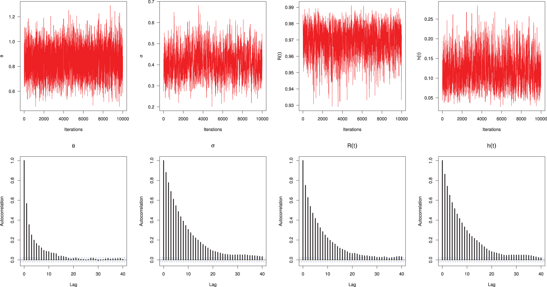
Figure 2: Trace (top) and Autocorrelation (bottom) plots for MCMC draws of θ, σ, R(t) and h(t) in Monte Carlo simulation

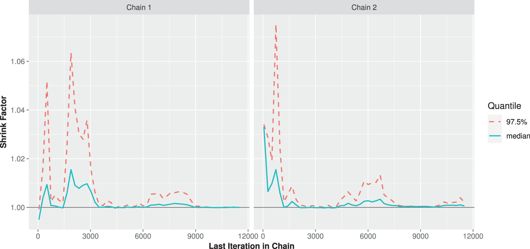
Figure 3: The BGR diagnostic for MCMC draws of θ (left) and σ (right) in Monte Carlo simulation

The average estimates (Av.Es) from classical (or Bayesian) approach of θ, σ, R(t) and h(t) (say ω) are given by:

ωˇd¯=11,000∑i=11,000ωˇd(i), d=1,2,3,4,

where ωˇ(i) is the calculated estimate of ω at the ith simulated sample, ω1=θ, ω2=σ, ω3=R(t) and ω4=h(t).

Further, the comparison between point estimates of ω is made based on their root mean squared-errors (RMSEs) and mean relative absolute biases (MRABs) as:

RMSE(ωˇd)=11000∑i=11000(ωˇd(i)−ωd)2, d=1,2,3,4,

and

MRAB(ωˇd)=11000∑i=110001ωd|ωˇd(i)−ωd|, d=1,2,3,4,

respectively.

Furthermore, the comparison between interval estimates of the same unknown parameters is made using their average confidence lengths (ACLs) and coverage percentages (CPs) which can be computed as

ACL(1−α)%(ωd)=11000∑i=11000(𝒰ωˇd(i)−ℒωˇd(i)), d=1,2,3,4,

and

CP(1−α)%(ωd)=11000∑i=110001(ℒωˇd(i);𝒰ωˇd(i))(ωd), d=1,2,3,4,

respectively, where 1(⋅) is the indicator function and ℒ(⋅) and 𝒰(⋅) denote the lower and upper bounds, respectively, of (1−α)% asymptotic (or HPD credible) interval of ωd.

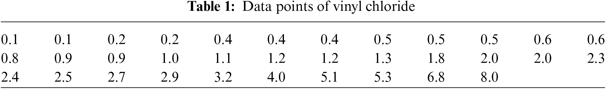
Heatmap is a method of representing data graphically where values are depicted by color, making it easy to visualize complex data and understand it at a glance. So, via R data visualization, all numerical results of θ, σ, R(t) and h(t) are displayed with heatmap plots in Figs. 4–7, respectively. Here, following the graphical tools reported in Elshahhat [18], the suggested heatmaps are plotted via R 4.1.2 software. Each heatmap range is classified from lowest to highest values with the colors cyan, red, and yellow, respectively. Each heatmap also displays the proposed estimation methods and the specified test settings on the “x-axis” and “y-axis” lines, respectively. In the supplementary file, all simulation tables of θ, σ, R(t) and h(t) are listed. Furthermore, for specification, several notations of the estimation methods have been used in Figs. 4–7 such as (based on Prior 1 (say P1) as an example) the Bayesian estimates based on SE loss mentioned as “SE-P1” as well as the Bayesian estimates based on GEnt loss for μ=−2 and +2 mentioned as “GE1-P1” and “GE2-P1”, respectively.

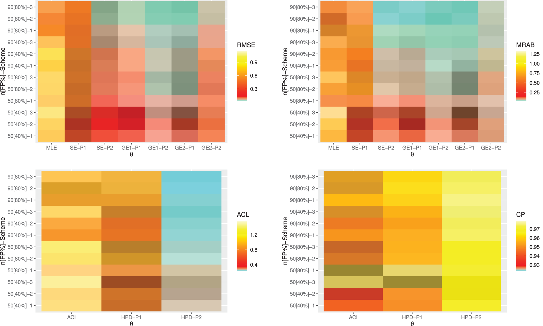
Figure 4: Heatmap plots for the point and interval results of θ

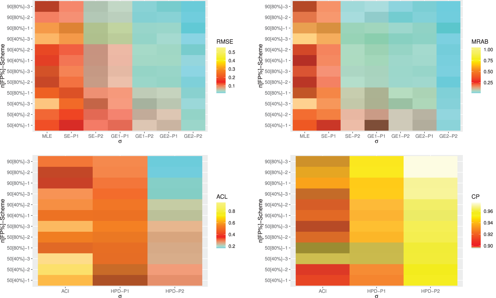
Figure 5: Heatmap plots for the point and interval results of σ

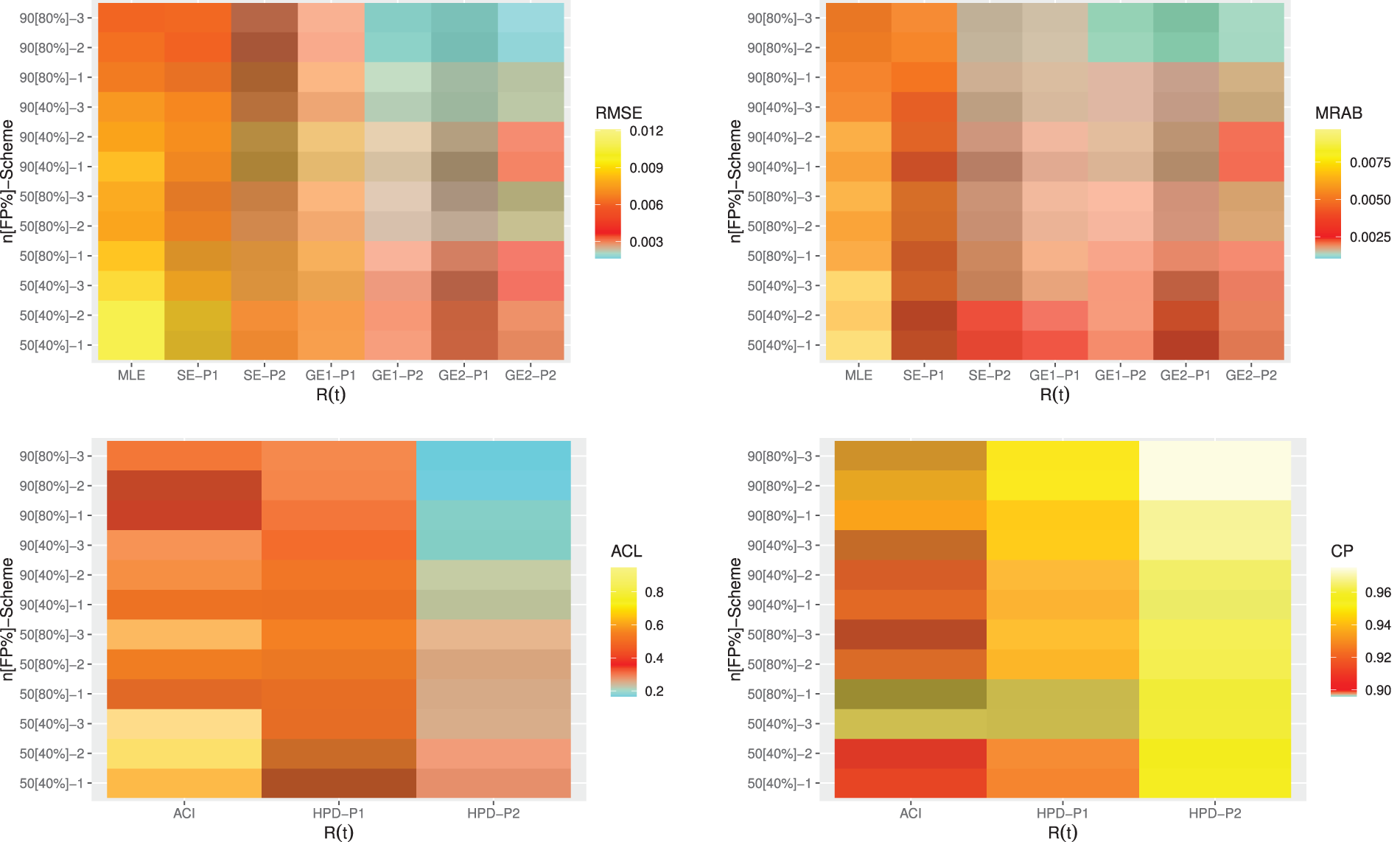
Figure 6: Heatmap plots for the point and interval results of R(t)

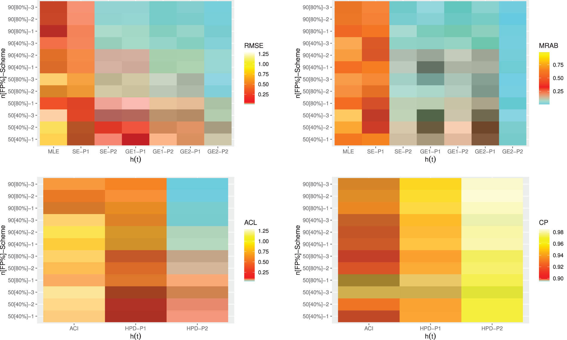
Figure 7: Heatmap plots for the point and interval results of h(t)

From Figs. 4–7, in terms of the lowest RMSE, MRAB and ACL values as well as the highest CP values, the following comments can be drawn:

•   Generally, the proposed point and interval estimates of θ, σ, R(t) and h(t) of the MOL model in presence of PT-IIC data behave satisfactorily.

•   As n(or FP) increases, the maximum likelihood and Bayesian estimates of θ, σ, R(t) and h(t) perform well. A similar observation is reached when n−m decreases.

•   Bayesian estimates against the GEnt loss function perform superior than those obtained against the SE loss function, and both perform better compared to the other estimates due to the gamma prior information. Similar result is also observed in the case of HPD credible interval estimates.

•   To evaluate the effect of parameter loss, it can be seen that the asymmetric Bayes estimates of θ, σ, R(t) or h(t) are overestimates (or underestimates) for μ<0 (or μ>0). This is one of the useful properties of working with the GEnt loss function.

•   Comparing the considered prior sets 1 and 2, due to the variance of prior 2 is smaller than the variance of prior 1, it is observed that the Bayesian estimates and associated HPD credible intervals under prior 2 of all unknown parameters have good perform than others.

•   Asymmetric Bayesian estimates of θ, σ, R(t) or h(t) have overestimates (when (μ<0)) and underestimates (when (μ>0)).

•   Comparing the censoring schemes 1, 2 and 3, it is clear that the both proposed point and interval estimates of θ and h(t) perform better using scheme-1 (when the survived items n−m drawn at x1); of R(t) perform better using scheme-3 (when the survived items n−m drawn at xm); and of σ perform better based on scheme-1 (for likelihood inference) while based on scheme-3 (for Bayesian inference).

•   Finally, to estimate the MOL distribution parameters or its reliability characteristics under PT-IIC mechanism, the Bayesian M-H algorithm method is recommended.

5  Real-Life Applications

In order to demonstrate the significance of the suggested inferential methodologies and the applicability of study objectives to actual phenomena, this part presents two practical applications from the domains of engineering and chemistry.

5.1 Vinyl Chloride

Vinyl chloride is a known human carcinogen and a rapidly burning colorless gas. In this application, 34 data points (measured in milligrams/liter) as presented in see Table 1 for vinyl chloride were taken from clean-up-gradient monitoring wells and analyzed. This data set was reported by Bhaumik et al. [19] and re-analyzed also by Elshahhat et al. [20], Alotaibi et al. [21], Elshahhat et al. [22].

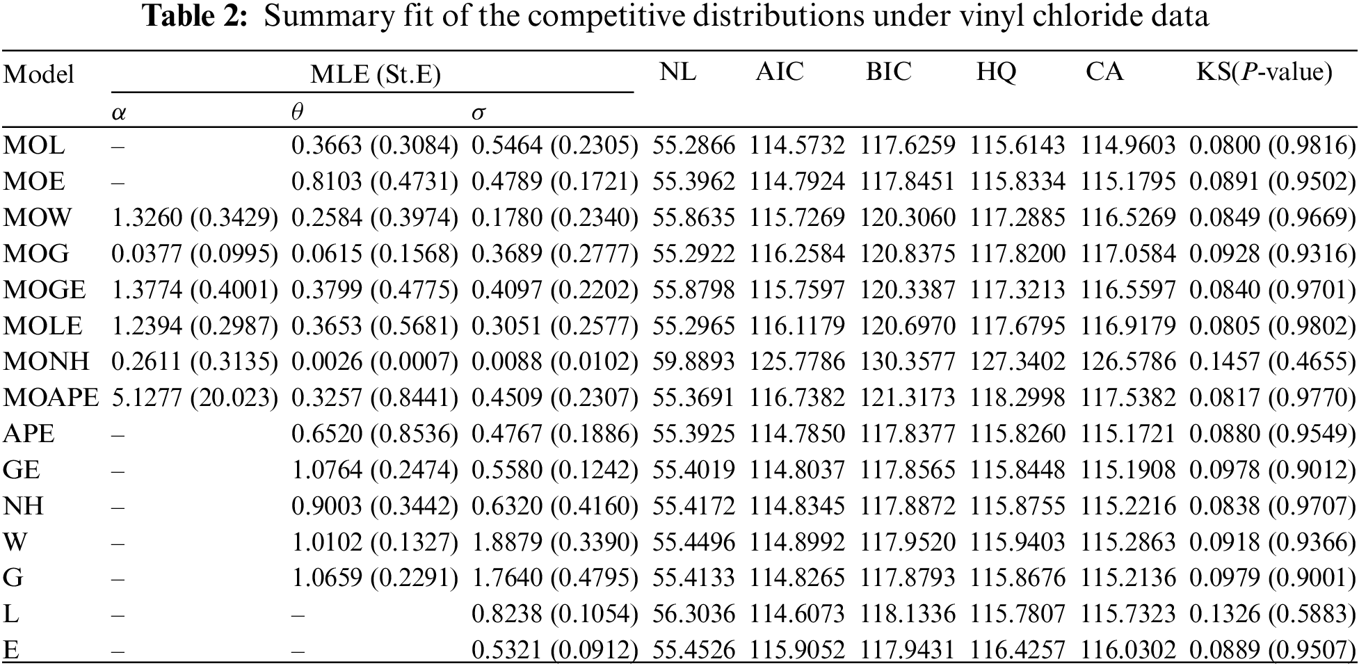
To verify the flexibility of the MOL model, the MOL distribution is compared with fourteen well-known distributions, (for x>0 and α,θ,σ), namely; Marshall-Olkin exponential (MOE(θ,σ)) by Marshall et al. [23], Marshall-Olkin Weibull (MOW(α,θ,σ)) by Cordeiro et al. [24], Marshall-Olkin Gompertz (MOG(α,θ,σ)) by Eghwerido et al. [25], Marshall-Olkin generalized exponential (MOGE(α,θ,σ)) by Ristić et al. [26], Marshall-Olkin logistic-exponential (MOLE(α,θ,σ)) by Mansoor et al. [27], Marshall-Olkin Nadarajah-Haghighi (MONH(α,θ,σ)) by Lemonte et al. [28], Marshall-Olkin alpha power exponential (MOAPE(α,θ,σ)) by Nassar et al. [29], alpha power exponential (APE(θ,σ)) by Mahdavi et al. [30], generalized-exponential (GE(θ,σ)) by Gupta et al. [31], Nadarajah-Haghighi (NH(θ,σ)) by Nadarajah et al. [32], Weibull (W(θ,σ)) by Weibull [33], gamma (G(θ,σ)) and exponential (E(σ)) by Johnson et al. [34], Lindley (L(σ)) by Lindley [35] distributions.

Different goodness-of-fit metrics, including the negative log-likelihood (NL), Akaike information criterion (AIC), Bayesian information criterion (BIC), Hannan-Quinn (HQ), Consistent Akaike (CA), and Kolmogorov-Smirnov (KS) statistic with its p-value, must be taken into account when comparing two (or more) distributions. The given goodness criteria are computed using the maximum likelihood and its standard-error (St.E) of each unknown parameter, as shown in Table 2. It is evident that the MOL distribution offers a better fit than other rival distributions based on the lowest values of NL, AIC, BIC, HQ, CA, and KS as well as the greatest p-value.

We also provided the quantile-quantile (QQ) plot as a graphical demonstration, via R 4.1.2 software, for each considered model, see Fig. 8. It is observed, from Fig. 8, that dots are not too far away from the diagonal line follow the diagonal line. It also supports the same results established in Table 2.

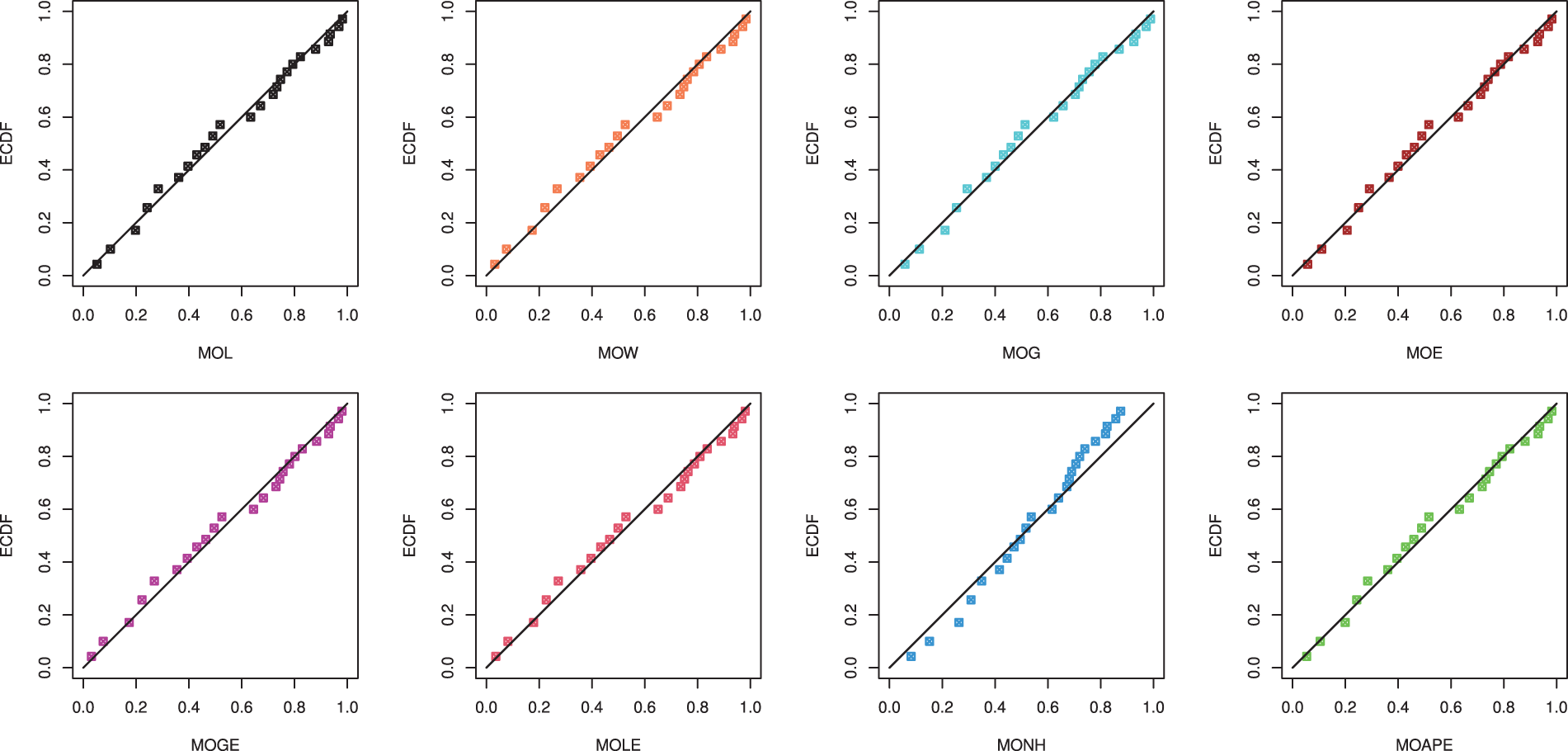
Figure 8: The Q-Q plots of the MOL and some competing distributions from vinyl chloride data

In Fig. 9, via R 4.1.2 software, we provided the histograms with the fitted densities as well as plots of the fitted and empirical RFs. Fig. 9a shows that the fitted density lines captured the data histograms adequately. Fig. 9b displays that the fitted reliability line of the proposed model captures the empirical reliability line better than others.

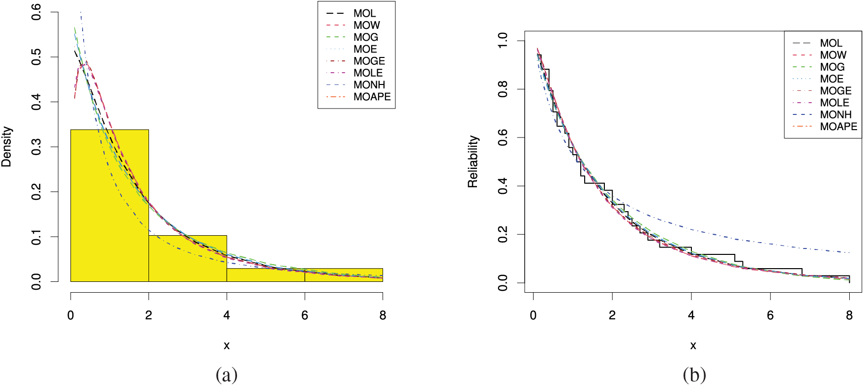
Figure 9: (a) Histograms and fitted PDFs and (b) Empirical and fitted RFs under vinyl chloride data

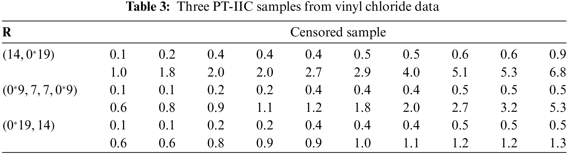
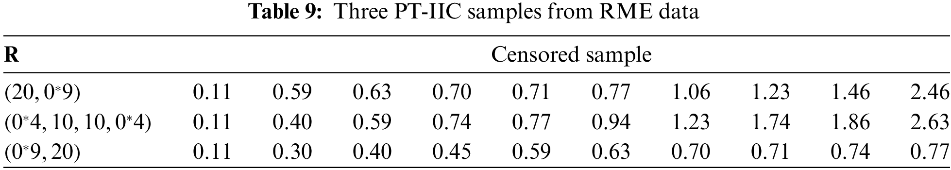
Now three different PT-IIC samples, from the complete vinyl chloride data, are generated with m=20 based on different schemes and reported in Table 3. From Table 3, the MLEs with their St.Es of θ, σ, R(t) and h(t) (at time t=0.2) are computed. via the M-H algorithm, from 50,000 MCMC samples with 10,000 burn-in, the Bayesian estimates with their St.Es under SE and GEnt (for μ(=−3,−0.03,+3)) loss functions of θ, σ, R(t) and h(t) (at t=0.2) are calculated using the improper priors, see Table 4. Also, in Table 5, the two bounds of the 95% ACI/HPD credible interval estimates with their lengths of the unknown parameters are also calculated. The classical estimates of θ and σ are selected as the start guesses to apply the proposed MCMC sampler. Before proceeding to calculate the Bayes objectives, we calculate the acceptance rate of Metropolis-Hastings proposals for all created samples, obtained by (14,0∗19), (0∗9,7,7,0∗9), and (0∗19,14) are: 60.294%, 57.774%, and 60.702%, respectively. It is observed that each MCMC sample gives an acceptable approximation for the posterior density, thus the derived inferences are reliable.

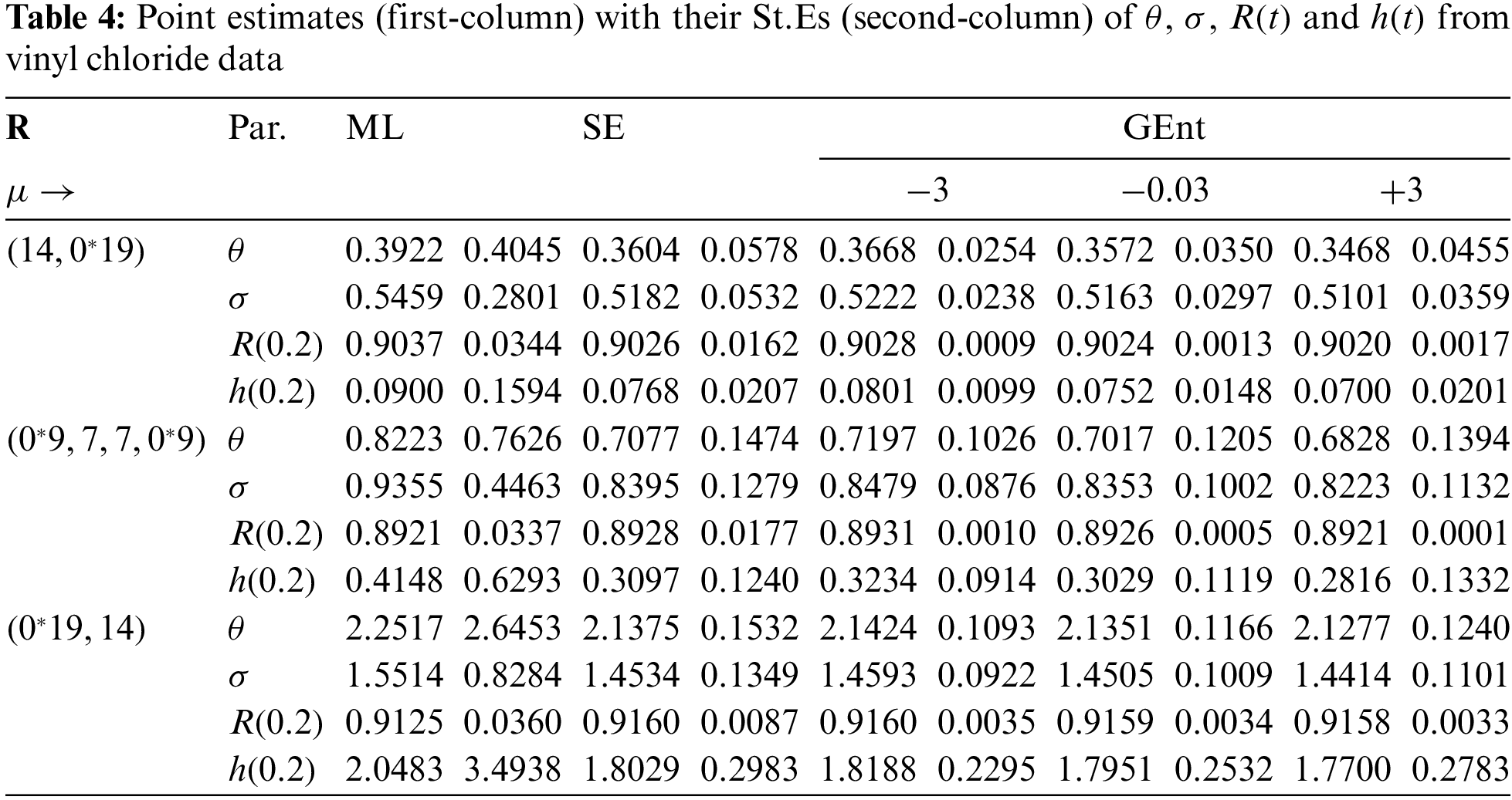
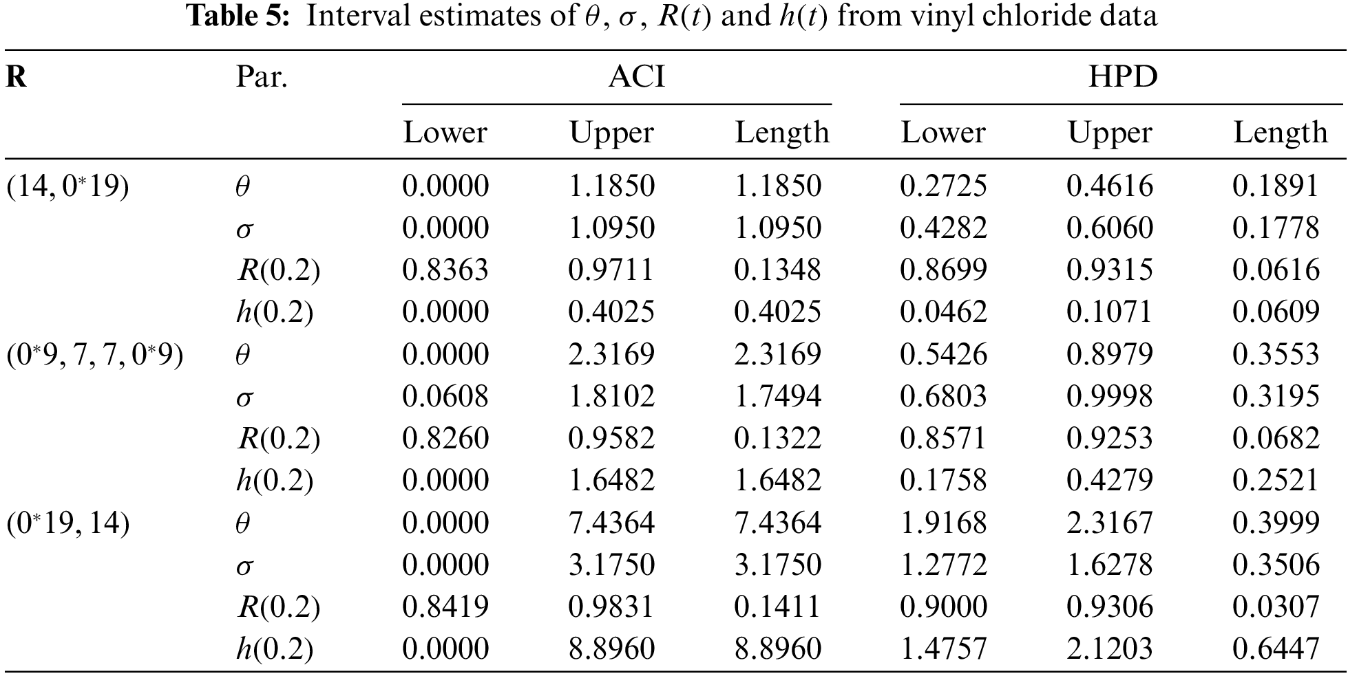
From each sample in Table 3, useful statistics for the MCMC variates of θ, σ, R(0.2) and h(0.2) after bun-in, namely: mean, mode, standard deviation (St.D), skewness and quartiles (Q1,Q2,Q3) are computed and presented in Table 6. To show the convergence of MCMC variates, based on the sample obtained from (14,0∗19) (as an example), MCMC trace plots of θ, σ, R(t) and h(t) are displayed in Fig. 10. Using the fitted Gaussian kernel for the sample obtained from (14,0∗19), the associated histograms of the simulated MCMC variates of θ, σ, R(t) and h(t) are also displayed in Fig. 10. All plots shown in Fig. 10 are developed via R 4.1.2 software.

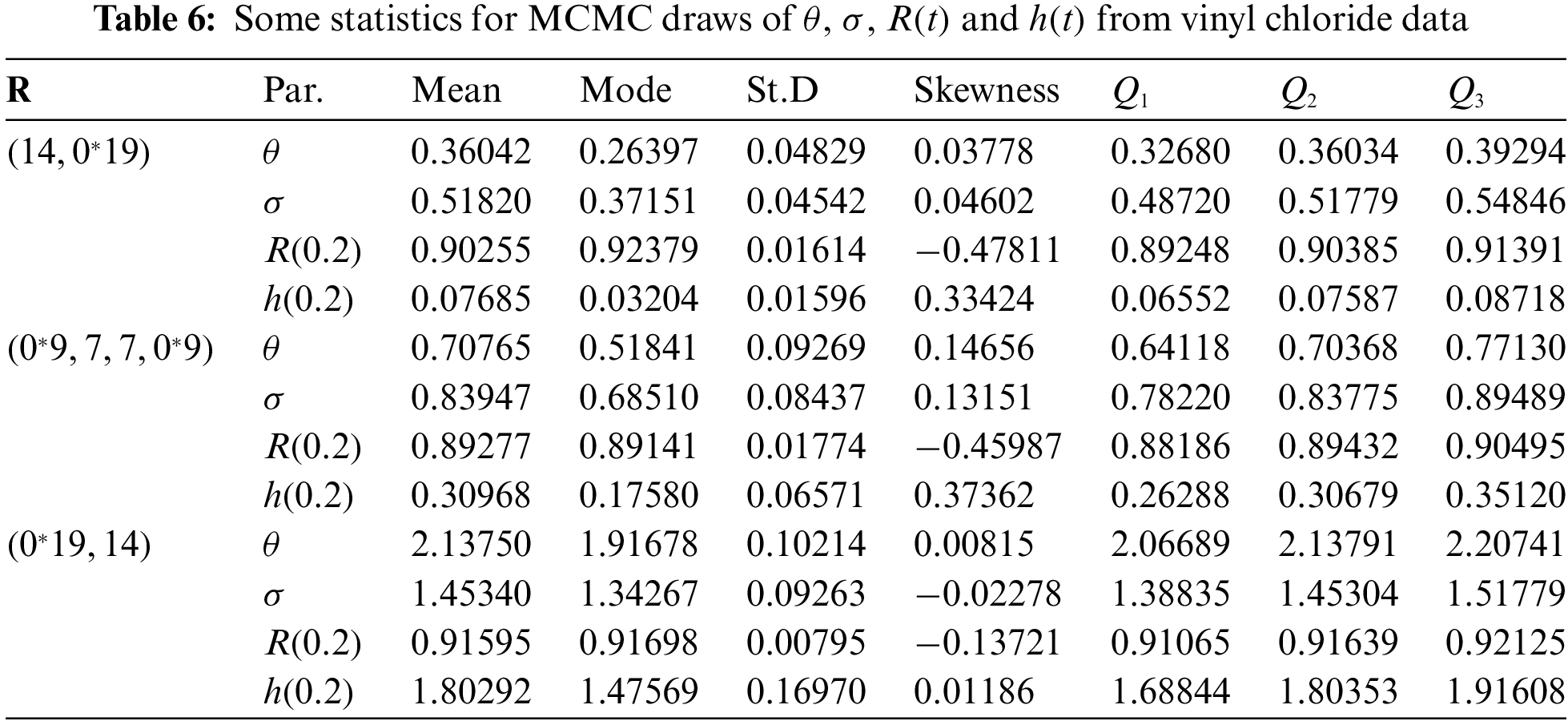
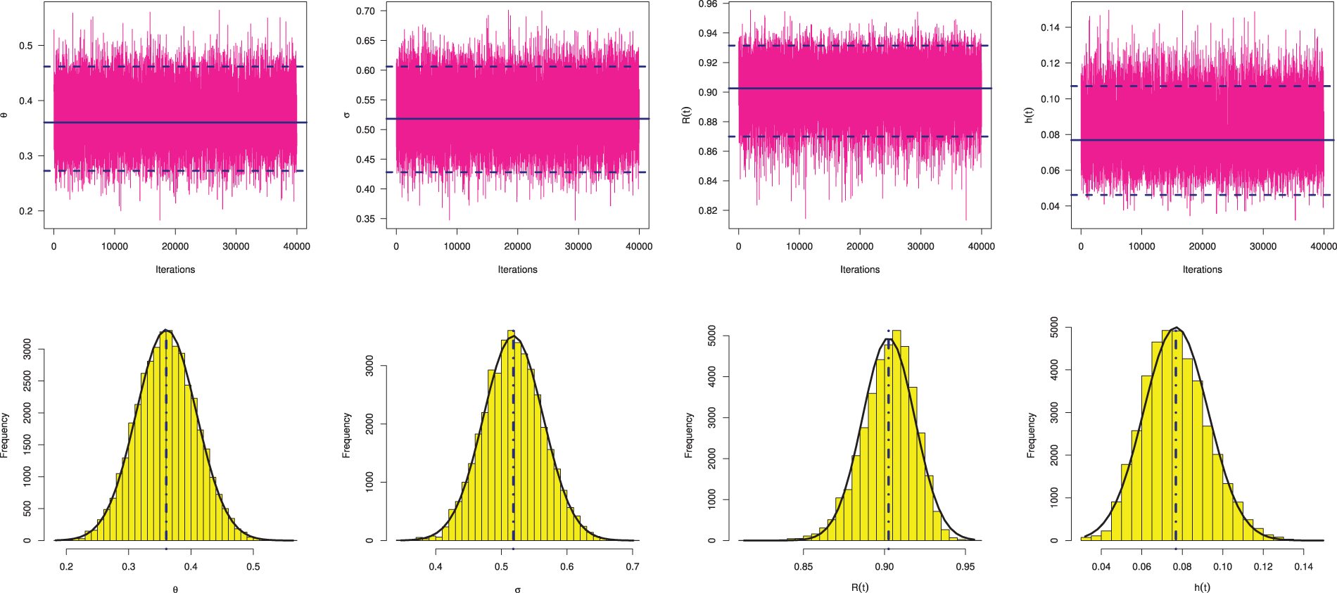
Figure 10: Trace (top) and Histograms (bottom) plots of θ, σ, R(t) and h(t) from vinyl chloride data

In each trace plot, the sample mean and two bounds of 95% HPD credible intervals of θ, σ, R(t) or h(t) are represented with soled- and dashed-horizontal lines, respectively. Additionally, each sample mean of θ, σ, R(t) or h(t) is represented with vertical dotted (:) line. Fig. 10 shows that the MCMC sampler converges quite well and indicates the burn-in sample has an appropriate size to eliminate the effect of the initial values. It is also observed, from Fig. 10, that the generated MCMC variates of θ and σ are fairly symmetrical while of R(t) and h(t) are negative and positive quite skewed, respectively. For brevity, other trace and histogram plots of θ, σ, R(t) and h(t) based on the PT-IIC samples obtained from (0∗9,7,7,0∗9) and (0∗19,14) are plotted and reported in the supplementary file.

5.2 Mechanical Equipments

In this application, from the engineering field, we will explain our theoretical results based on the time between consecutive failures for repairable mechanical equipment (RME) items depicted in Table 7. Murthy et al. [36] initially conveyed this data and it has also been examined by Elshahhat et al. [37], Nassar et al. [38], and Elshahhat et al. [39]. Employing the competitive statistical distributions as well as the model selection criteria proposed in Subsection 5.1, the MOL distribution based on the complete RME data is compared. All results of the MOL distribution and other models are provided in Table 8. It suggests that the MOL distribution is the most suitable model to fit the MRE data when compared to others.

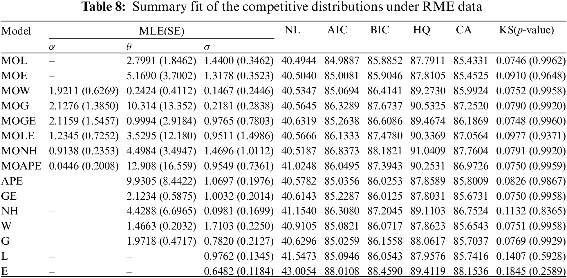
Also, using the complete RME data, Fig. 11 displays the QQ plots of MOL, MOE, MOW, MOG, MOGE, MOLE, MONH and MOAPE distributions. It supports the same findings reported in Table 8 also. Further, three graphics of goodness-of-fit are investigated; (i) plot of histograms of RME data with fitted PDFs, and (ii) plot of the fitted and empirical RFs under RME data are shown in Fig. 12. It indicates that the MOL distribution is the best model compared to its competitive models.

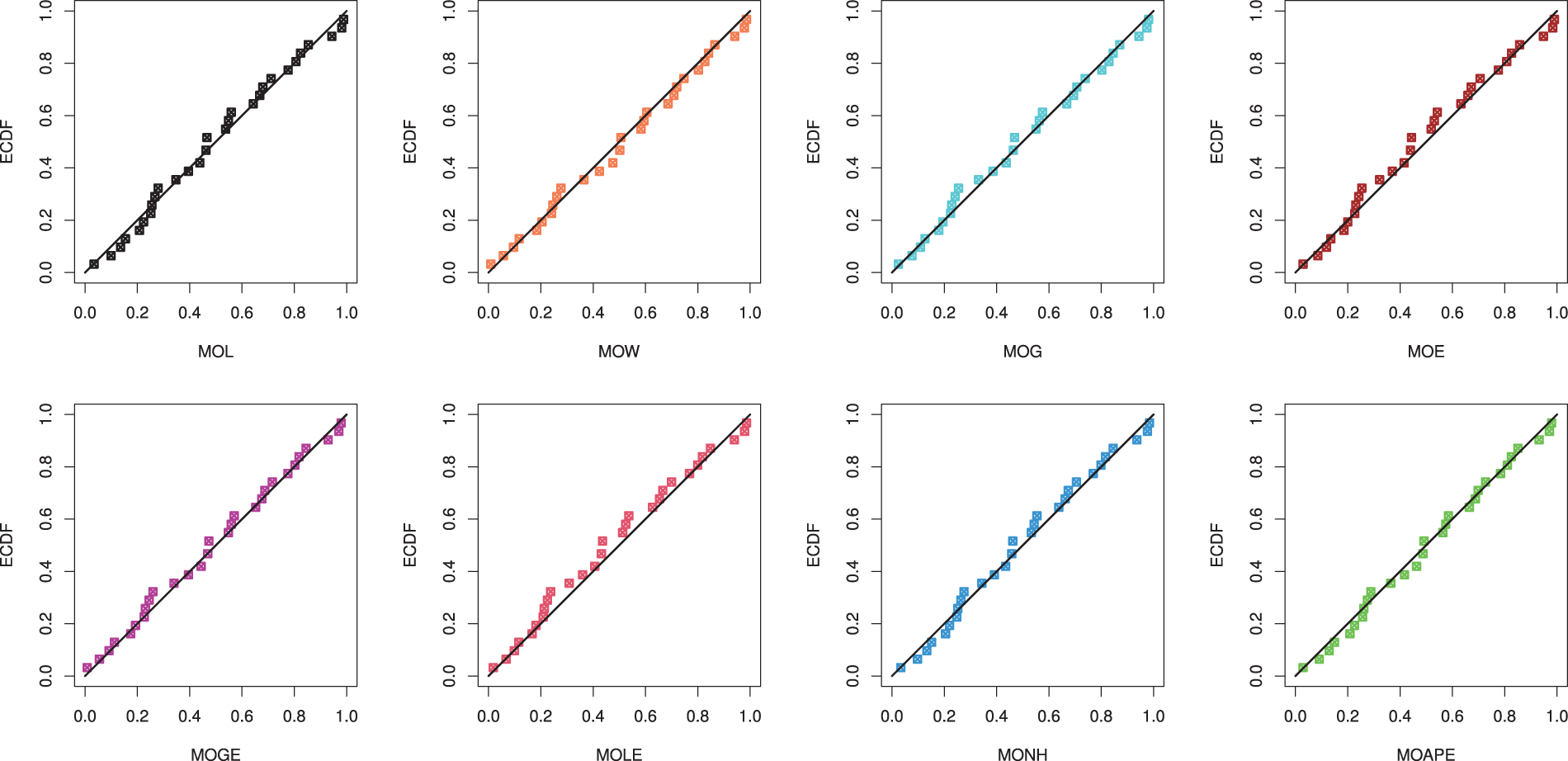
Figure 11: The Q-Q plots of the competing models from mechanical equipments data

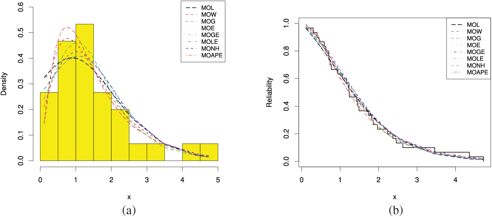
Figure 12: (a) Histograms and fitted PDFs and (b) Empirical and fitted RFs from the RME data

From the complete RME data, three different PT-IIC samples are generated with m=10 based on different schemes and provided in Table 9. From each generated sample in Table 9, the maximum likelihood and Bayesian estimates with their St.Es of θ, σ, R(t) and h(t) (at time t=0.5) are computed and presented in Table 10. Two-sided 95% ACI and HPD credible interval estimates with their lengths of θ, σ, R(t) and h(t) are also calculated and reported in Table 11. Via improper priors, utilizing 50,000 MCMC draws with 10,000 burn-in, the Bayesian analysis is performed based on both SE and GEnt (for μ(=−5,−0.05,+5)) (Table 12). Using the PT-IIC samples generated by (20,0∗9), (0∗4,10,10,0∗4) and (0∗9,20), the acceptance rates of the Metropolis-Hastings proposals are 61.824%, 61.132%, and 61.154%, respectively. These rates support the same result reported in Application 5.1, which is that the percentage of iterations in which the proposals were accepted is much higher.

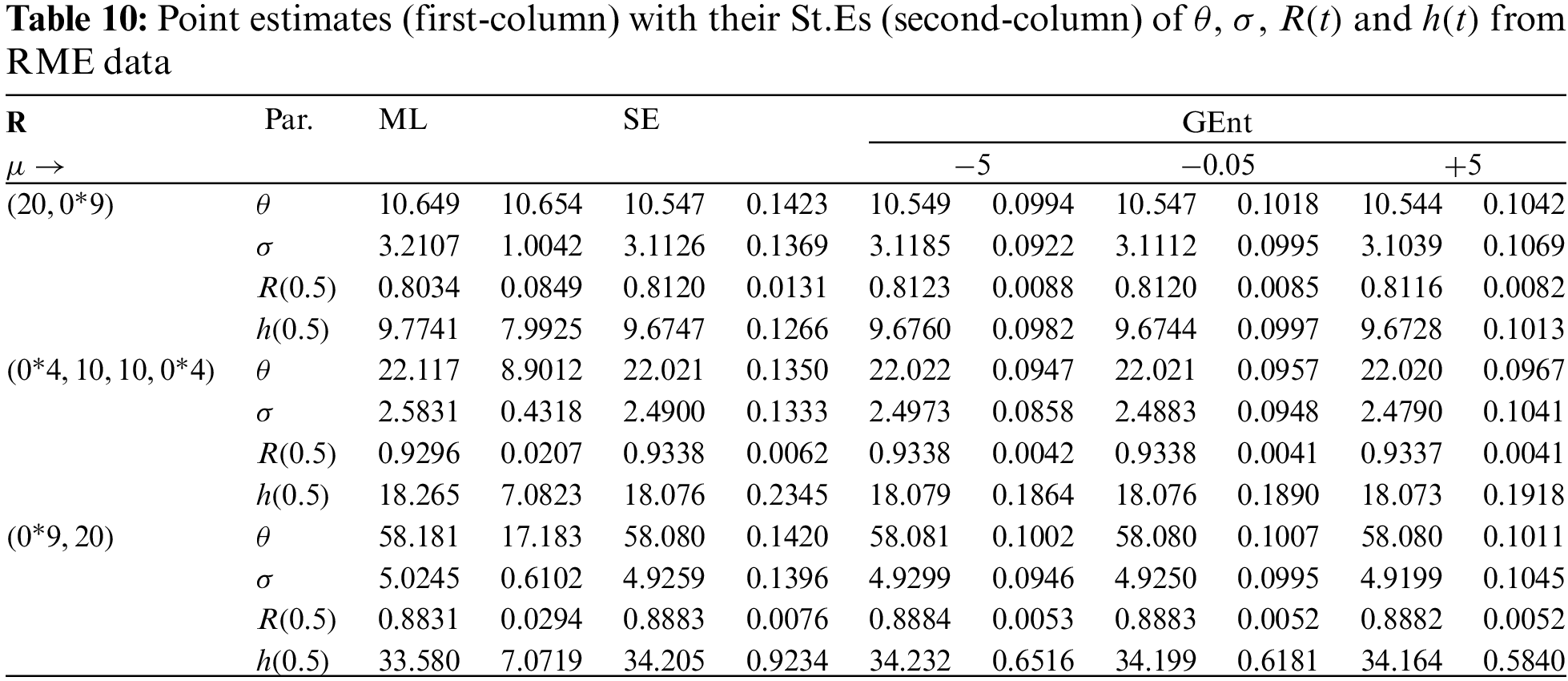
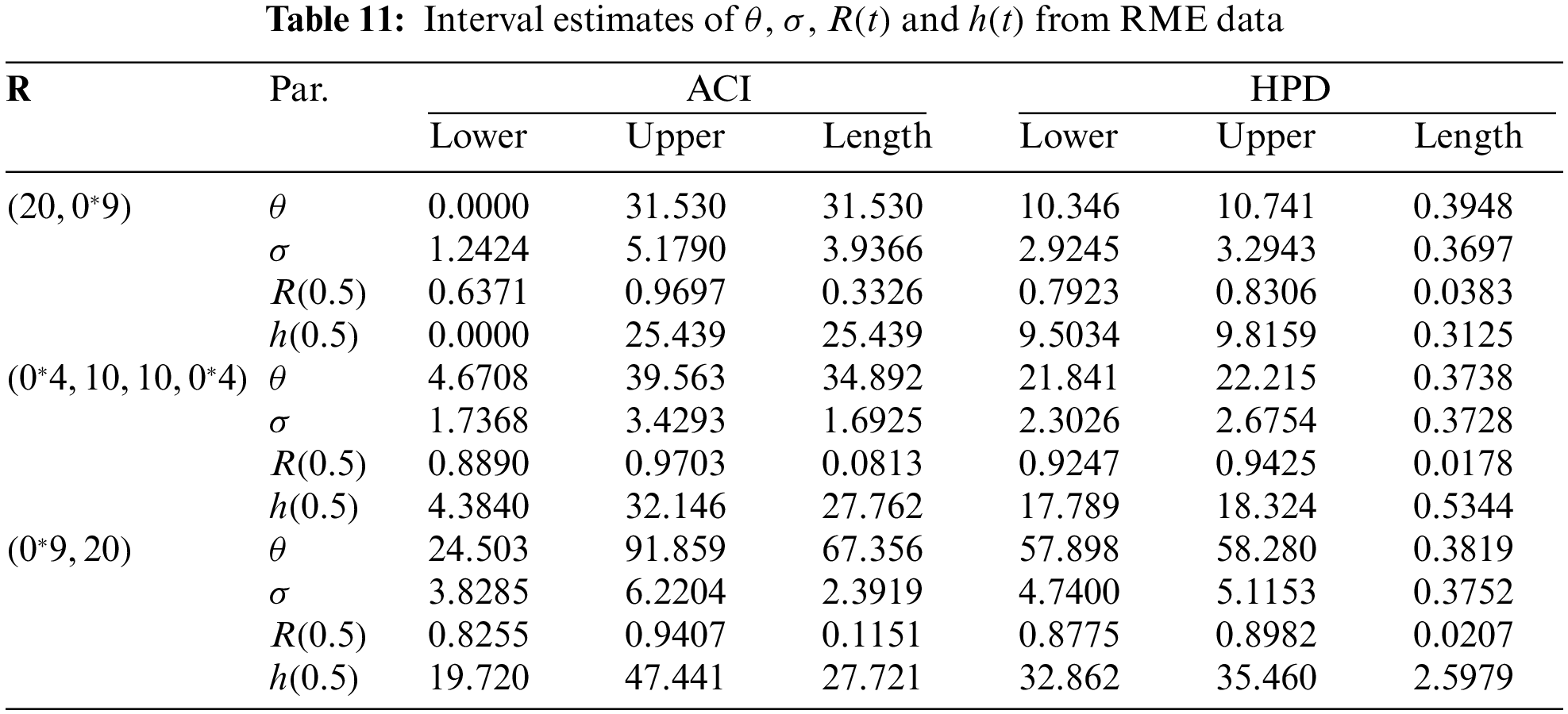
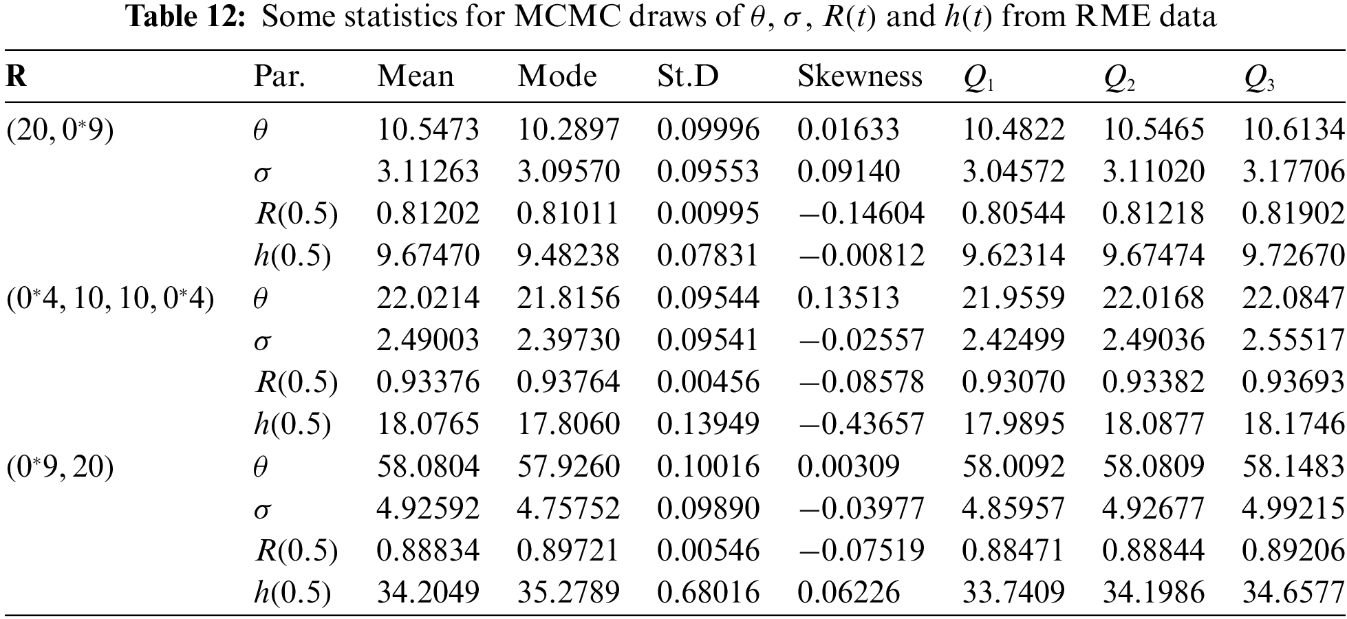
From the PT-IIC sample generated by (20,0∗9), trace and histogram plots of the MCMC simulated variates of all unknown parameters are provided in Fig. 13. It shows that the MCMC mechanism converges well and demonstrates that the MCMC variates of θ, σ, R(t) and h(t) are fairly symmetrical. Other plots of θ, σ, R(t) and h(t) based on (0∗4,10,10,0∗4) and (0∗9,20) are available in the supplementary file. Lastly, from both chemical and engineering examples, one can decide that the results of the proposed methodologies provide a good explanation to the proposed MOL lifetime model.

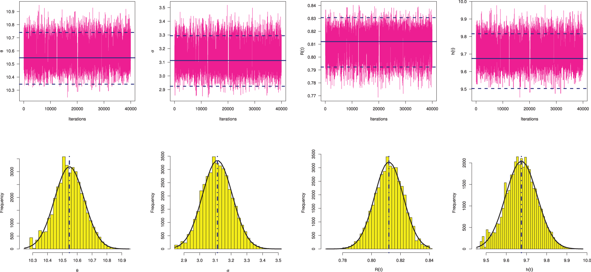
Figure 13: Trace (top) and Histograms (bottom) plots of θ, σ, R(t) and h(t) from RME data

6  Concluding Remarks

In this study, we looked into the statistical inference of the Marshall-Olkin Lindley distribution’s unknown parameters, reliability, and hazard rate functions under progressively Type-II censored data. The various parameters of interest are inferred using both classical and Bayesian methods. The normal approximation of the maximum likelihood estimators is also used to create the approximate confidence intervals. The Bayesian estimations are addressed by employing independent gamma priors and symmetric and asymmetric loss functions. We have indicated that the explicit expressions of the proposed Bayesian estimators are not available. The Markov Chain Monte Carlo technique is employed as a result. For each parameter, the highest posterior density credible intervals are also attained. We conducted a thorough simulation analysis and examined two applications to real-world data sets to evaluate the effectiveness of the delivered estimations. The findings of the numerical study showed that when progressively Type-II censored data were given, the suggested point and interval estimations of the Marshall-Olkin Lindley distribution acted reasonably. More specifically, the highest posterior density credible intervals were advised and the Bayesian estimates utilizing the general entropy loss function outperformed all other estimates. In addition, the real data analysis showed that the Marshall-Olkin Lindley distribution could be used as a good model to fit vinyl chloride and repairable mechanical equipment data sets rather than some other Marshall-Olkin models, including Marshall-Olkin Weibull, Marshall-Olkin Gompertz, Marshall-Olkin generalized exponential and Marshall-Olkin logistic-exponential distributions. In future work, it is of interest to investigate the estimation problems of the considered distribution based on other censoring schemes like an adaptive progressive Type-II censoring scheme. Another significant future work to be addressed is exploring the performance of dependability metrics of the utilized model in the case of accelerated life tests.

Acknowledgement: The authors would desire to express their thanks to the editor and the three anonymous referees for useful suggestions and valuable comments. Princess Nourah bint Abdulrahman University Researchers Supporting Project and Princess Nourah bint Abdulrahman University, Riyadh, Saudi Arabia.

Funding Statement: This research was funded by Princess Nourah bint Abdulrahman University Researchers Supporting Project Number (PNURSP2023R50), Princess Nourah bint Abdulrahman University, Riyadh, Saudi Arabia.

Author Contributions: The authors confirm contribution to the paper as follows: study conception and design: R. Alotaibi, M. Nassar, and A. Elshahhat; data collection: A. Elshahhat; analysis and interpretation of results: A. Elshahhat; draft manuscript preparation: M. Nassar, R. Alotaibi. All authors reviewed the results and approved the final version of the manuscript.

Availability of Data and Materials: The data that support the findings of this study are available in the text.

Conflicts of Interest: The authors declare that they have no conflicts of interest to report regarding the present study.

Supplementary Materials: The supplementary material is available online at https://doi.org/10.32604/cmes.2023.030582.

References

1. Ghitany, M. E., Al-Mutairi, D. K., Al-Awadhi, F. A., Al-Burais, M. M. (2012). Marshall-Olkin extended Lindley distribution and its application. International Journal of Applied Mathematics, 25(5), 709–721. [Google Scholar]

2. do Espirito Santo, A. P. J., Mazucheli, J. (2015). Comparison of estimation methods for the Marshall-Olkin extended Lindley distribution. Journal of Statistical Computation and Simulation, 85(17), 3437–3450. [Google Scholar]

3. Balakrishnan, N., Aggarwala, R. (2000). Progressive censoring: Theory, methods, and applications. Birkhäuser, Boston: Springer Science & Business Media. [Google Scholar]

4. Balakrishnan, N., Cramer, E. (2014). The art of progressive censoring. Birkhäuser, New York: Springer. [Google Scholar]

5. Sultan, K. S., Alsadat, N. H., Kundu, D. (2014). Bayesian and maximum likelihood estimations of the inverse Weibull parameters under progressive type-II censoring. Journal of Statistical Computation and Simulation, 84(10), 2248–2265. [Google Scholar]

6. Guo, L., Gui, W. (2018). Statistical inference of the reliability for generalized exponential distribution under progressive type-II censoring schemes. IEEE Transactions on Reliability, 67(2), 470–480. [Google Scholar]

7. Joukar, A., Ramezani, M., MirMostafaee, S. M. T. K. (2020). Estimation of P (X > Y) for the power Lindley distribution based on progressively type II right censored samples. Journal of Statistical Computation and Simulation, 90(2), 355–389. [Google Scholar]

8. Elshahhat, A., Rastogi, M. K. (2021). Estimation of parameters of life for an inverted Nadarajah-Haghighi distribution from Type-II progressively censored samples. Journal of the Indian Society for Probability and Statistics, 22(1), 113–154. [Google Scholar]

9. Alotaibi, R., Nassar, M., Rezk, H., Elshahhat, A. (2022). Inferences and engineering applications of alpha power Weibull distribution using progressive Type-II censoring. Mathematics, 10(16), 2901. [Google Scholar]

10. Okasha, H., Nassar, M. (2022). Product of spacing estimation of entropy for inverse Weibull distribution under progressive type-II censored data with applications. Journal of Taibah University for Science, 16(1), 259–269. [Google Scholar]

11. Maiti, K., Kayal, S., Kundu, D. (2022). Statistical Inference on the shannon and rényi entropy measures of generalized exponential distribution under the progressive censoring. SN Computer Science, 3(4), 1–21. [Google Scholar]

12. Calabria, R., Pulcini, G. (1994). An engineering approach to Bayes estimation for the Weibull distribution. Microelectronics Reliability, 34(5), 789–802. [Google Scholar]

13. Henningsen, A., Toomet, O. (2011). maxLik: A package for maximum likelihood estimation in R. Computational Statistics, 26(3), 443–458. [Google Scholar]

14. Kundu, D. (2008). Bayesian inference and life testing plan for the Weibull distribution in presence of progressive censoring. Technometrics, 50(2), 144–154. [Google Scholar]

15. Dey, S., Elshahhat, A., Nassar, M. (2022). Analysis of progressive type-II censored gamma distribution. Computational Statistics, 38(1), 481–508. [Google Scholar]

16. Plummer, M., Best, N., Cowles, K., Vines, K. (2006). CODA: Convergence diagnosis and output analysis for MCMC. R News, 6, 7–11. [Google Scholar]

17. Roy, V. (2020). Convergence diagnostics for Markov Chain Monte Carlo. Annual Review of Statistics and Its Application, 7(1), 387–412. [Google Scholar]

18. Elshahhat, A. (2022). R programming language for data analytics. The 55th Annual International Conference on Data Science, Egypt, Cairo University. https://doi.org/10.13140/RG.2.2.15044.09607/1 [Google Scholar] [CrossRef]

19. Bhaumik, D. K., Kapur, K., Gibbons, R. D. (2009). Testing parameters of a gamma distribution for small samples. Technometrics, 51(3), 326–334. [Google Scholar]

20. Elshahhat, A., Elemary, B. R. (2021). Analysis for xgamma parameters of life under type-II adaptive progressively hybrid censoring with applications in engineering and chemistry. Symmetry, 13(11), 2112. [Google Scholar]

21. Alotaibi, R., Nassar, M., Elshahhat, A. (2022). Computational analysis of XLindley parameters using adaptive Type-II progressive hybrid censoring with applications in chemical engineering. Mathematics, 10(18), 3355. [Google Scholar]

22. Elshahhat, A., Dutta, S., Abo-Kasem, O. E., Mohammed, H. S. (2023). Statistical analysis of the Gompertz-Makeham model using adaptive progressively hybrid Type-II censoring and its applications in various sciences. Journal of Radiation Research and Applied Sciences, 16(4), 100644. https://doi.org/10.1016/j.jrras.2023.100644 [Google Scholar] [CrossRef]

23. Marshall, A. W., Olkin, I. (1997). A new method for adding a parameter to a family of distributions with application to the exponential and Weibull families. Biometrika, 84(3), 641–652. [Google Scholar]

24. Cordeiro, G. M., Lemonte, A. J. (2013). On the Marshall-Olkin extended Weibull distribution. Statistical Papers, 54(2), 333–353. [Google Scholar]

25. Eghwerido, J. T., Ogbo, J. O., Omotoye, A. E. (2021). The Marshall-Olkin Gompertz distribution: Properties and applications. Statistica, 81, 183–215. [Google Scholar]

26. Ristić, M. M., Kundu, D. (2015). Marshall-Olkin generalized exponential distribution. Metron, 73(3), 317–333. [Google Scholar]

27. Mansoor, M., Tahir, M. H., Cordeiro, G. M., Provost, S. B., Alzaatreh, A. (2019). The Marshall-Olkin logistic-exponential distribution. Communications in Statistics-Theory and Methods, 48(2), 220–234. [Google Scholar]

28. Lemonte, A. J., Cordeiro, G. M., Moreno-Arenas, G. (2016). A new useful three-parameter extension of the exponential distribution. Statistics, 50, 312–337. [Google Scholar]

29. Nassar, M., Kumar, D., Dey, S., Cordeiro, G. M., Afify, A. Z. (2019). The Marshall-Olkin alpha power family of distributions with applications. Journal of Computational and Applied Mathematics, 351, 41–53. [Google Scholar]

30. Mahdavi, A., Kundu, D. (2017). A new method for generating distributions with an application to exponential distribution. Communications in Statistics-Theory and Methods, 46(13), 6543–6557. [Google Scholar]

31. Gupta, R. D., Kundu, D. (1999). Theory and methods: Generalized exponential distributions. Australian and New Zealand Journal of Statistics, 41(2), 173–188. [Google Scholar]

32. Nadarajah, S., Haghighi, F. (2011). An extension of the exponential distribution. Statistics, 45(6), 543–558. [Google Scholar]

33. Weibull, W. (1951). A statistical distribution function of wide applicability. Journal of Applied Mechanics, 18(3), 293–297. [Google Scholar]

34. Johnson, N., Kotz, S., Balakrishnan, N. (1994). Continuous univariate distributions. 2nd edition. New York: John Wiley and Sons. [Google Scholar]

35. Lindley, D. V. (1958). Fiducial distributions and Bayes’ theorem. Journal of the Royal Statistical Society: Series B, 20, 102–107. [Google Scholar]

36. Murthy, D. N. P., Xie, M., Jiang, R. (2004). Weibull models. In: Wiley series in probability and statistics. New Jersey: John Wiley and Sons. [Google Scholar]

37. Elshahhat, A., Aljohani, H. M., Afify, A. Z. (2021). Bayesian and classical inference under Type-II censored samples of the extended inverse gompertz distribution with engineering applications. Entropy, 23(12), 1578. [Google Scholar] [PubMed]

38. Nassar, M., Elshahhat, A. (2023). Estimation procedures and optimal censoring schemes for an improved adaptive progressively type-II censored Weibull distribution. Journal of Applied Statistics. https://doi.org/10.1080/02664763.2023.2230536 [Google Scholar] [CrossRef]

39. Elshahhat, A., Almetwally, E. M., Dey, S., Mohammed, H. S. (2023). Analysis of WE parameters of life using adaptive-progressively Type-II hybrid censored mechanical equipment data. Axioms, 12(7), 690. [Google Scholar]