Fault Identification for Shear-Type Structures Using Low-Frequency Vibration Modes

1  Introduction

The shear-type structure is a common structural form in industrial and civil buildings, such as concrete and steel frame structures. For example, many high-rise residential buildings can be classified as the shear-type structures due to the particularly high stiffness of the floor compared to the columns. It is known that structural failures are inevitable due to the environmental corrosion, material fatigue, disaster loads, and other factors. In order to ensure residential safety, it is necessary to carry out structural health monitoring and defect diagnosis. Due to the large volume and numerous components of building structures, traditional non-destructive testing techniques such as ultrasound, radiographic testing, and penetration testing cannot complete defect diagnosis of large building structures. In the past few decades, methods for diagnosing structural damage using response parameters of structures under static or dynamic loads have been continuously studied in depth. The theoretical basis for this type of method is that faults in structures can cause changes in structural static and vibration response parameters [1–4]. In practice, the response data of structures can be measured through special testing equipment and then their changes can be used to diagnose structural fault conditions.

In recent years, many methods have been developed for structural fault diagnosis by using static or dynamic response parameters. Yang et al. proposed a fast static displacement analysis method for structural damage detection using flexible disassembly perturbation [5,6]. Peng et al. [7] developed a method for determining the damage location of beam structures by using redistribution of static shear energy. Li et al. [8] proposed a flexible method for damage identification of cantilever structures, such as high-rise buildings and chimneys, using a few dynamic modal data. Koo et al. [9] proposed a damage quantification method for shear buildings based on the modal data measured by ambient vibration. It is found from the experimental study that the damage quantity of the proposed method is very consistent with the actual damage quantity obtained from the static pushdown test. Zhu et al. [10] proposed an effective damage detection method for shear buildings by using the change of the first mode shape slope. An eight-layer numerical example and a three-layer experimental model verify the effectiveness of the method. Xing et al. [11] proposed a substructure method that allows local damage detection of shear structures. Their method only needs three sensors to identify the local damage of any floor of the shear structure building. The feasibility of the proposed method is tested by simulation and experiment on a five-storey building. Su et al. [12] developed a simple and effective method to locate the floors where the property (stiffness and mass) changes during the shear building life cycle. The floors that may be damaged are determined by comparing the natural frequencies of the substructure at different stages of the building life cycle. Sung et al. [13] conducted a comprehensive experimental verification of the damage induced deflection method for shear building damage detection. The results showed that the damaged floor was successfully located, and the damage rate estimated by the damage induced deflection method was consistent with the damage rate calculated by numerical simulation. Panigrahi et al. [14] developed a method based on residual force vector and genetic algorithm to identify damages of multi-layer shear structures from sparse modal information. Li et al. [15] proposed a data-driven method for seismic damage detection and location of multi-degree-of-freedom shear-type building structures under strong ground motions. The proposed method is based on the joint realization of time-frequency analysis and fractal dimension characteristics. An et al. [16] carried out the application research of damage location method based on impact energy in real-time damage detection of shear structures under random base excitation. The performance of their method in damage detection was experimentally verified using a laboratory scale 6-layer shear structure model. Wang et al. [17] proposed a damage identification method for the shear-type building based on proper orthogonal modes. The experimental results show that this method can effectively identify the location and severity of shear building structure damage. Mei et al. [18] proposed an improved substructure based damage detection method to locate and quantify damage in shear structures. Luo et al. [19] proposed a new method for extracting the spectral transfer function and detecting damage of shear frame structures under non-stationary random excitation. Shi et al. [20] studied the damage localization by using the curvature of the lateral displacement envelope in the shear building structure. The finite difference method and interpolation method are used to evaluate the modal curvature and frequency response function for damage localization. Mei et al. [21] presented a new substructure damage detection method based on the autoregressive moving average exogenous input (ARMAX) model and the optimal sub-mode assignment (OSPA) distance to locate and quantify the damage. Paral et al. [22] proposed a damage assessment method based on artificial neural network, which takes the change of the first mode slope damage index as the input layer of the artificial neural network. The effectiveness of their method is proved by the experimental tests of the three-story steel shear frame model. Liang et al. [23] carried out the damage detection of shear buildings by frequency-change-ratio and model updating algorithm. Ghannadi et al. [24] used a new bio-inspired optimization algorithm to identify the damage location and severity of the multi-layer shear frame. Do et al. [25] developed a new damage detection method based on output-only vibration information for shear-type structures. Zhao et al. [26] proposed a two-step modeling method based on wavelet frequency response function estimation and least squares iterative algorithm to identify structural vibration modal parameters. Liu et al. [27] studied schemes to repair earthquake damage from the aspects of load transfer path, enclosure structure, beam column nodes, and structural stiffness. It was found that the seismic performance of masonry walls can be greatly improved after being wrapped in reinforced concrete or seismic zones. Niu [28] proposed a damage detection method for shear frame structures based on frequency response function. The influence of noise on damage detection is greatly suppressed by simultaneously increasing the number of equations and reducing the unknown coefficients. Yang et al. [29,30] studied dynamic model reduction and used modal sensitivity for fault diagnosis based on the reduced model. Tan et al. [31] proposed a model- calibration-free method for damage identification of shear structures using modal data. The advantage of the proposed method is that the model-free calibration characteristics can avoid the need to calibrate the mass and stiffness parameters of the structure. Roy [32] proposed a new formula to establish the expression of damage severity in the form of mode shape slope. The derived closed-form solution directly relates the percentage of damage strength to the derivative of the vibration mode change in the shear building.

Although great progress has been made in damage diagnosis of shear structures, there are still many difficulties that need to be further studied to overcome. The main disadvantage of the existing methods described above is that accurate structural finite element model (FEM) is required in these methods to perform the damage assessment. However, it is difficult to obtain accurate FEMs for many shear-type structures. It is an urgent need in engineering practice to study defect diagnosis methods that do not require accurate finite element models. For this purpose, a FEM-free method for defect diagnosis of the shear structure is developed in this paper, which only needs to measure a few low-order vibration modes of the structure. The proposed defect diagnosis method is divided into two stages. In the first stage, the location of the defect is determined based on the virtual displacement difference derived from the dynamic flexibility matrix before and after damage. In the second stage, the damage severity is evaluated based on the improved frequency sensitivity equation. The main innovations of the proposed method lie in two aspects. The first is the development of a virtual displacement difference method for determining the location of damage in the shear structure. The second is to improve the existing frequency sensitivity equation to calculate the damage degree without constructing FEM. The proposed method has been validated on a numerical model of a 22-story shear-type frame structure and a three-story steel shear structure model. Based on numerical analysis and experimental data validation, it is shown that the proposed method can diagnose the defect location and damage degree only by using the lower order modes of structural vibration, and does not require finite element modeling. The proposed method should be a very simple and practical defect diagnosis technique in engineering practice.

2  Theoretical Development

2.1 Damage Localization by the Virtual Displacement Difference

In this section, the virtual displacement difference method is proposed for defect localization of shear-type structures. For an undamaged structure with n degrees of freedom (DOFs), the free vibration modes can be computed by the following generalized eigenvalue problem as:

(K−λrM)φr=0(1)

φrTMφr=1(2)

where K and M are the stiffness and mass matrices of the FEM of the undamaged structure, λr is the r-th eigenvalue (angular frequency), φr is the mass-normalized eigenvector (mode shape). Note that λr and φr (also called as the r-th eigen-pair) can be also obtained by the dynamic test on the undamaged structure without FEM. A structure with n-DOFs will have n independent eigen-pairs, i.e., r=1∼n. Thus Eqs. (1) and (2) can be rewritten for n eigen-pairs as:

KΨ=MΨΛ(3)

ΨTMΨ=I(4)

where I is a n-dimensional identity matrix, Ψ is the eigenvector matrix and Λ is the eigenvalue matrix as:

Ψ=[φ1,⋯,φn](5)

Λ=[λ1⋱λn](6)

From Eq. (4), one has

Ψ−1=ΨTM(7)

(ΨT)−1=MΨ(8)

Combining Eq. (3) with (7), one has

K=MΨΛΨTM(9)

From Eq. (9), the inverse matrix of K (i.e., the flexibility matrix F) can be obtained as:

F=K−1=(ΨTM)−1Λ−1(MΨ)−1(10)

Using Eqs. (7), (8), and (10) can be simplified as:

F=K−1=ΨΛ−1ΨT(11)

Using Eqs. (5), (6) and (11) can be rewritten as:

F=K−1=∑r=1n1λrφrφrT(12)

The eigenvalues of structural vibration are generally sorted from small to large, that is, 0<λ1<λ2<λ3<⋯. This means that the reciprocal ordering of eigenvalues is exactly the opposite as 1λ1>1λ2>1λ3>⋯>0. Thus Eq. (12) can be approximated as:

F≈∑r=1m1λrφrφrT(13)

where m is the number of the lower-frequency modes in the dynamic test of the undamaged structure. It is known that the appearance of structural defects usually only results in changes in structural stiffness or flexibility, while the mass generally does not change. For a damaged structure, the similar equations can be derived as follows:

(Kd−λdrM)φdr=0(14)

φdrTMφdr=1(15)

Fd=Kd−1=∑r=1n1λdrφdrφdrT(16)

Fd≈∑r=1m1λdrφdrφdrT(17)

in which Kd is the stiffness matrix of the damaged system, λdr and φdr are the corresponding eigenvalue and mode shape, Fd is the damage flexibility matrix. Note that λdr and φdr can be also obtained by the dynamic test on the damaged structure without FEM. From Eqs. (13) and (17), the change of the dynamic flexibility matrix due to fault can be approximately computed by:

ΔF≈∑r=1m(1λdrφdrφdrT−1λrφrφrT)(18)

From a static perspective, the displacement before and after structural damage under a certain static load can be obtained as follows:

ξ=F⋅lv(19)

ξd=Fd⋅lv(20)

where ξ and ξd are the displacement vectors before and after structural damage under the certain static load lv. For shear-type structures, it can be assumed that a unit force is applied at the free end of the structure to obtain a virtual load vector of lv=(1,0,0,⋯,0)T. Note that the purpose of applying a unit force at the free end of the shear structure is to ensure that each layer of the structure can undergo shear deformation, as shown in Fig. 1a. If this unit force is applied to the middle layer, the layers above the load position will not undergo shear deformation, as shown in Fig. 1b. Thus the loading scheme of Fig. 1b will not be able to identify the possible damage in the layers above the load location by the shear deformation. In view of this, the virtual load should be applied to the free end of the shear structure (i.e., the top layer) as shown in Fig. 1a. Note that in Fig. 1a, the floors are numbered from top to bottom as 1, 2, … , n. Thus the virtual load vector corresponding to Fig. 1a is lv=(1,0,0,⋯,0)T since only the element corresponding to the unit force at the first floor is 1 and the other elements are zeros. If the floors are numbered from bottom to top as 1, 2, … , n, as shown in Fig. 1c, the corresponding virtual load vector will be lv=(0,0,⋯,0,1)T since only the element corresponding to the unit force at the highest floor is 1 and the other elements are zeros.

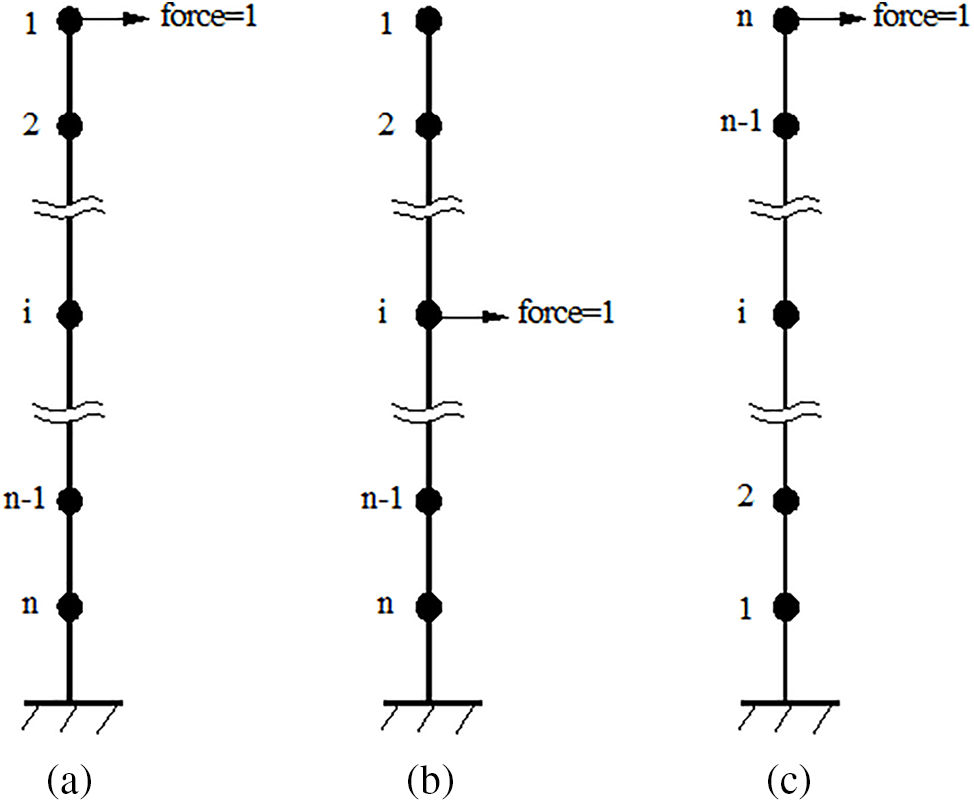
Figure 1: (a) A virtual load at the top floor (floors are numbered from top to bottom as 1, 2, … , n); (b) A virtual load at the middle layer; (c) A virtual load at the top floor (floors are numbered from bottom to top as 1, 2, … , n)

Therefore, the virtual displacement difference vector Δξ can be obtained as:

Δξ=ΔF⋅lv(21)

According to the research results of the reference [33], it has been proven that the displacement difference vector for the linear structure before and after damage under the same static load will undergo a sudden change at the damage location. Thus the location of the fault in a shear structure can be determined by the location of the element value mutation in the vector Δξ. The virtual displacement difference vector Δξ is also called as the defect localization vector. It should be emphasized that the vector Δξ can be obtained from Eq. (21) only by testing the low-frequency modal data of the free vibration of the shear structure before and after damage, without requiring a finite element model. This means that the defect localization of the structure can be carried out without the need to establish a FEM of the structure in advance.

2.2 Damage Quantification by the Improved Frequency Sensitivity

An assessment of the defect severity is necessary to estimate the remaining life of the structure or to determine whether maintenance is required. To this end, an improved frequency sensitivity algorithm is developed for fault quantification of the shear structure. According to the FEM theory, the total stiffness matrix K of the undamaged structure can be obtained by the sum of all the elementary stiffness matrices as:

K=∑i=1NKi(22)

where Ki is the i-th elementary stiffness matrix, N is the number of all elements of the structure. In most cases, structural damage only leads to a decrease in structural stiffness without causing a change in mass. The reduction in local stiffness can be represented by multiplying a reduction coefficient by the elementary stiffness matrix. Therefore, the total stiffness matrix considering structural damage can be expressed as:

K=∑i=1N(1+εi)Ki(23)

where εi is a reduction coefficient reflecting the severity of the defect in the i-th element. εi is a number located in the interval [−1, 0]. Theoretically, εi=0 denotes that the i-th element has not been damaged, −1<εi<0 indicates partial damage to the i-th element, and εi=−1 indicates complete damage to the i-th element. By performing partial derivatives on Eq. (1) with respect to the variable εi, one has:

(K−λrM)∂φr∂εi=(∂λr∂εiM−Ki)φr(24)

in which ∂λr∂εi and ∂φr∂εi are the frequency and mode shape sensitivities, respectively. Eq. (1) can be rewritten by the matrix transpose as:

[(K−λrM)φr]T=0(25)

According to the FEM theory, the stiffness and mass matrices K and M are both symmetric matrices. Thus Eq. (25) can be expanded by considering the symmetry of K and M as:

φrT(K−λrM)=0(26)

Multiplying Eq. (24) by φrT and using Eq. (26), one has

0=φrT(∂λr∂εiM−Ki)φr(27)

Eq. (27) can be expanded as:

∂λr∂εi(φrTMφr)=φrTKiφr(28)

Substituting Eq. (2) into (28) yields

∂λr∂εi=φrTKiφr(29)

The eigenvalue (i.e., angular frequency) variation Δλr due to the faults in the structure can be calculated by:

Δλr=λdr−λr(30)

Substituting Eq. (23) into (1) yields as:

(∑i=1N(1+εi)Ki−λrM)φr=0(31)

Eq. (31) shows that λr is a implicit function of the variables ε1,ε2,⋯,εN, i.e., λr=f(ε1,ε2,⋯,εN). Thus the change of λr due to the changes of ε1,ε2,⋯,εN can be approximated by using Taylor’s series expansion and ignoring higher-order derivatives as:

Δλr=∑i=1Nεi∂λr∂εi(32)

As stated before, the defect location has been determined based on the damage location vector Δξ in the first stage. The following quantitative evaluation of defects is divided into two situations: single defect and multiple defects. For single defect case, assuming that the i-th element is determined to be a damaged element, Eq. (32) is simplified as:

Δλr=εi∂λr∂εi(33)

Substituting Eq. (29) into (33) yields

Δλr=εi(φrTKiφr)(34)

In the above derivation, φr is the mass-normalized mode shape obtained by solving the eigenvalue problem based on structural FEM. To avoid constructing FEM, Eq. (34) can be improved by replacing the mode shape calculated from FEM with the tested mode shape as:

Δλr=εi(φ¯rTKiφ¯r)(35)

where φ¯r represents the measured mode shape of the undamaged structure. Generally, the first vibration mode is the easiest to measure and has the highest accuracy. Thus the fault coefficient can be calculated using the first vibration mode from Eq. (35) as:

εi=Δλ1φ¯1TKiφ¯1(36)

Note that Ki in Eq. (36) can be directly obtained by the interlayer stiffness of the i-th element of the shear structure without the need to establish structural FEM. It is known that the elementary stiffness matrix of the shear structure in local co-ordinates can be expressed as:

Kie=12EIL3[1−1−11](37)

where E denotes the elastic modulus, I denotes the moment of inertia, L is the shear element length, and 12EIL3 is also called as the interlayer stiffness. Eqs. (36) and (37) indicate that the fault coefficient of the structure can be solved directly using the tested vibration mode and the interlayer stiffness of the individual element, without the need to construct a FEM of the entire structure.

For multiple defect case, more vibration modes besides the first vibration mode are needed to solve the fault coefficients. The number of the used vibration modes should be greater than or equal to the number of damage locations determined by the above damage localization approach. Without losing generality, Eq. (32) can be expanded for multiple defects to

[Δλ1⋮Δλm]=S⋅{εi⋮εj}(38)

S=[∂λ1∂εi⋯∂λ1∂εj⋮⋱⋮∂λm∂εi⋯∂λm∂εj](39)

where the matrix S is also obtained by using the measured mode shapes instead of the theoretical mode shapes computed by FEM. This improvement can avoid establishing the overall FEM of the structure. From Eq. (38), all the fault coefficients can be computed by:

{εi⋮εj}=S+[Δλ1⋮Δλm](40)

In Eq. (40), the superscript “+” denotes the matrix generalized inverse. Finally, the damage severity of shear structures can be evaluated based on the calculation results of Eq. (40). Fig. 2 shows the flow chart of the proposed algorithm to explain the process more clearly.

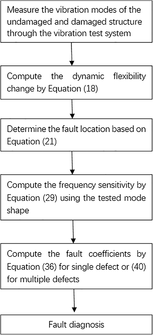
Figure 2: Flowchart of the proposed algorithm

3  Validation by the Numerical Model

A 22-story shear frame structure shown in Fig. 3a is used to verify the feasibility of the presented approach. The stiffness and mass of each floor in Fig. 3a are k1=k2=1296, k3=⋯=k22=1024, m1=m2=72, and m3=⋯=m22=64, respectively. The node numbers from the ground to the roof of this shear structure are 1, 2, ... , and 23, as shown in Fig. 3b. Two defect scenarios are simulated in this numerical example. The first defect scenario assumes a 15% reduction in the interlayer stiffness of the fifth floor. The second defect scenario assumes that the stiffness of the 5th and 16th floors is reduced by 20% and 15%, respectively. Note that the reduction of interlayer stiffness is achieved through the reduction of stiffness parameter ki. For example, k5 = 1024 of the undamaged structure changes to be k5 = 0.85 × 1024 = 870.4 of the damaged structure, resulting in a 15% reduction in the interlayer stiffness of the fifth floor for the first defect scenario. In this example, only the first and second vibration modes are used for defect diagnosis. A 3% level of data noise is added to the vibration modes of the damaged structure to simulate the measurement errors. Tables 1 and 2 present the eigen-frequencies and modal shapes obtained by the FEMs of the undamaged and damaged structures. Note that the node number is different from the floor number as shown in Fig. 3b. The node 1 in Table 2 corresponds to the fixed end of the structure. For this numerical example, the frequencies and modal shapes are obtained from the FEM by solving the above eigenvalue in Eq. (1). The data with noise in these tables are used to simulate the corresponding values obtained from the dynamic test in a real scenario. Note that these modal data can be obtained through vibration testing experiments for a real scenario in practice. For example, the data used in the following experimental structure is the actual test data, as shown in the next section.

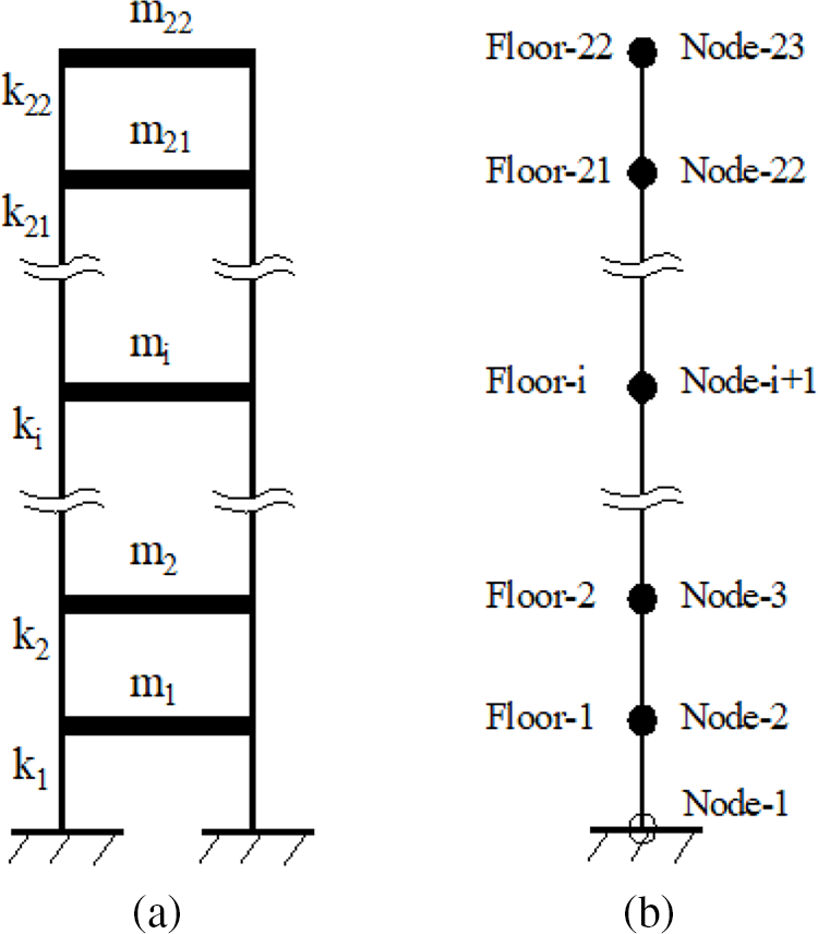
Figure 3: (a) A 22-story numerical shear frame structure; (b) Floor number and node number

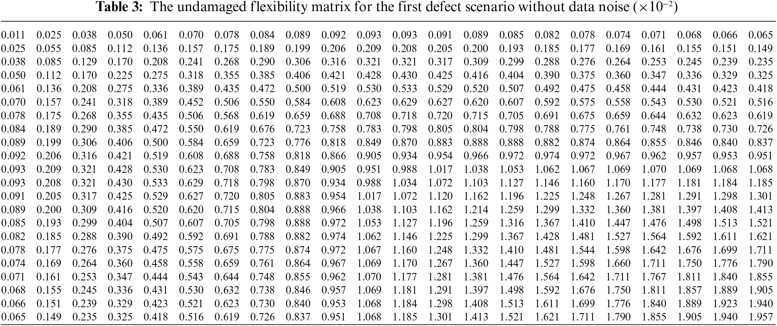
Taking the first defect scenario without data noise as an example, the specific process of calculating the damage localization vector Δξ using the proposed method is as follows:

(1) Calculate the undamaged flexibility matrix F using Eq. (13) as:

F≈1λ1φ1φ1T+1λ2φ2φ2T(41)

The result of F obtained by Eq. (41) is shown in Table 3.

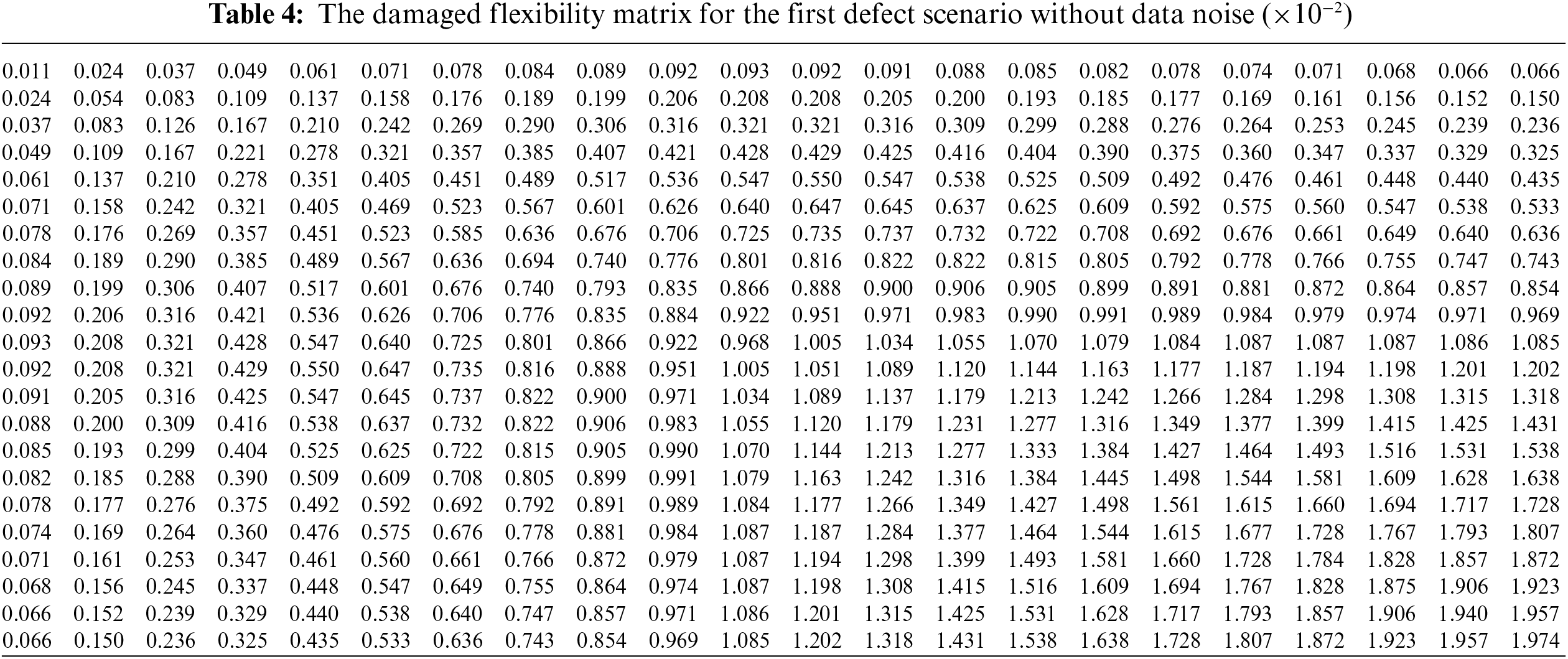
(2) Calculate the damaged flexibility matrix Fd using Eq. (17) as:

Fd≈1λd1φd1φd1T+1λd2φd2φd2T(42)

The result of Fd obtained by Eq. (42) is shown in Table 4.

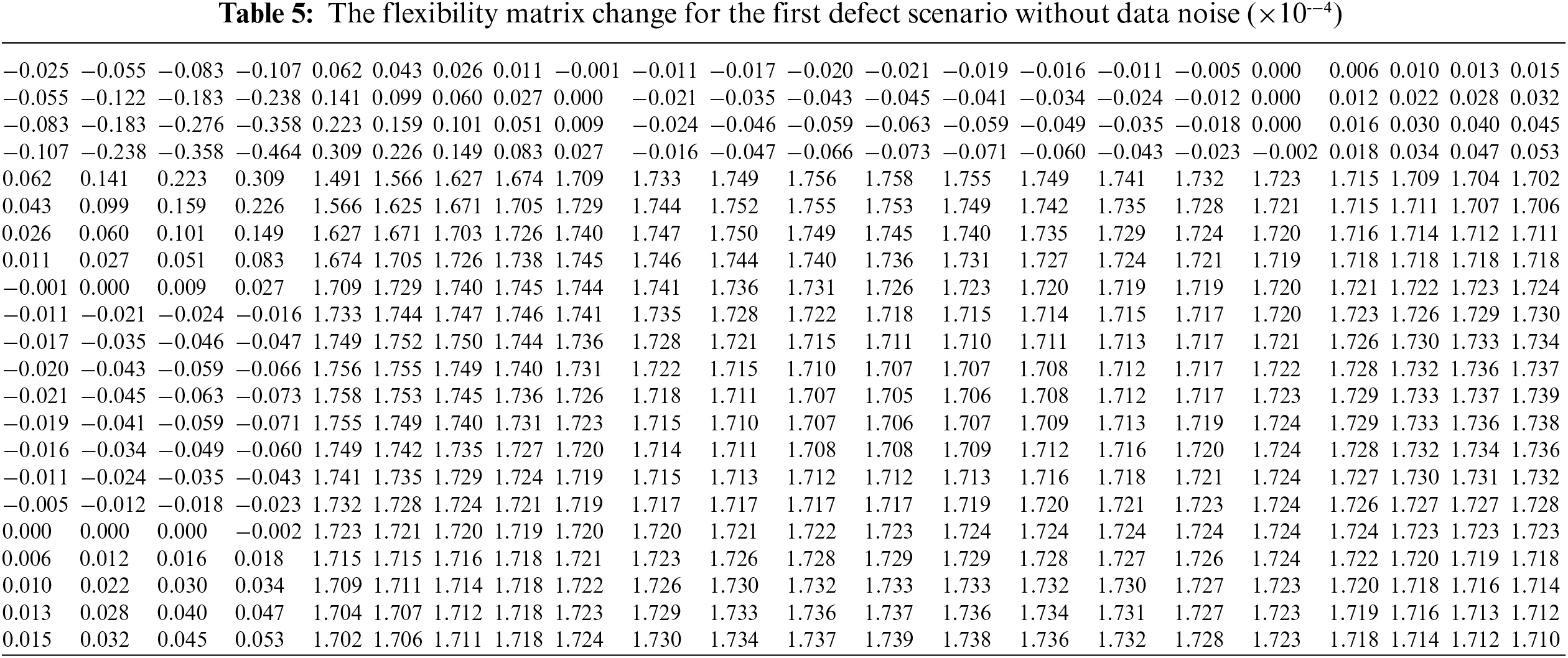
(3) Calculate the flexibility matrix change ΔF by:

ΔF=Fd−F(43)

The result of ΔF obtained by Eq. (43) is shown in Table 5.

(4) Calculate damage localization vector Δξ using Eq. (21) with lv=(0,0,0,0,0,0,0,0,0,0,0,0,0, 0,0,0,0,0,0,0,0,1)T. Fig. 4 gives the calculation result of the defect localization vector Δξ for the first defect scenario by the exact data and the data with 3% noise. From Fig. 4, one can find that there is a mutation between the nodes numbered 5 and 6, which exactly corresponds to the fifth floor. This means that the fifth floor is where the defect is located. For the second defect scenario, Fig. 5 gives the calculation results of the defect localization vectors by the exact data and the data with 3% noise. From Fig. 5, one can find that there is two mutations between the nodes numbered 5, 6, 16, and 17, which exactly correspond to the 5th and 16th floors. This means that the 5th and 16th floors are where the defects are located. For the above two defect scenarios, Table 6 presents the calculated severity of the damages using the data with and without noise. One can find from Table 6 that these calculated damage severity values are relatively close to the assumed true values in the two defect scenarios. This indicates that the proposed method can successfully determine the locations and extents of the defects in this numerical shear structure.

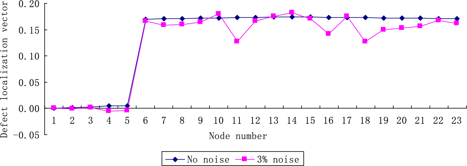
Figure 4: The defect localization vector Δξ for the first defect scenario of the numerical example when the fifth floor is damaged (×10−3)

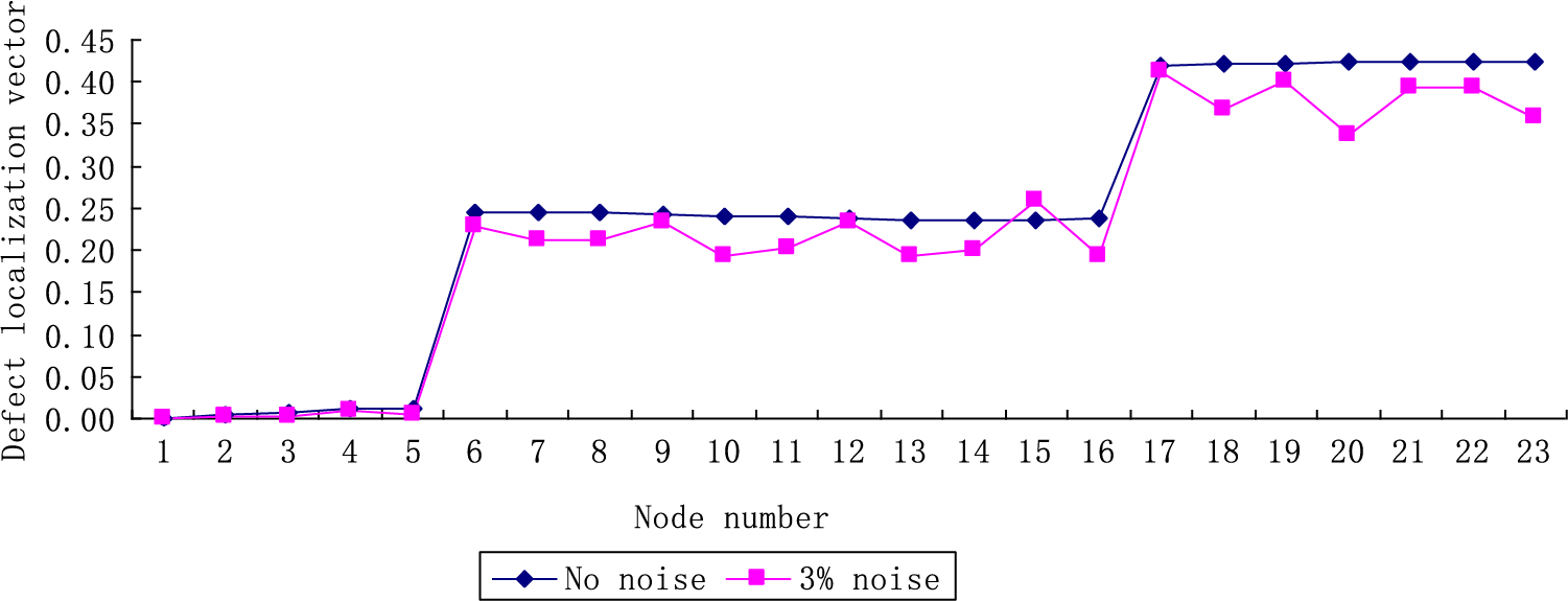
Figure 5: The defect localization vector Δξ for the second defect scenario of the numerical example when the 5th and 16th floors are damaged (×10−3)

4  Validation by Experimental Data

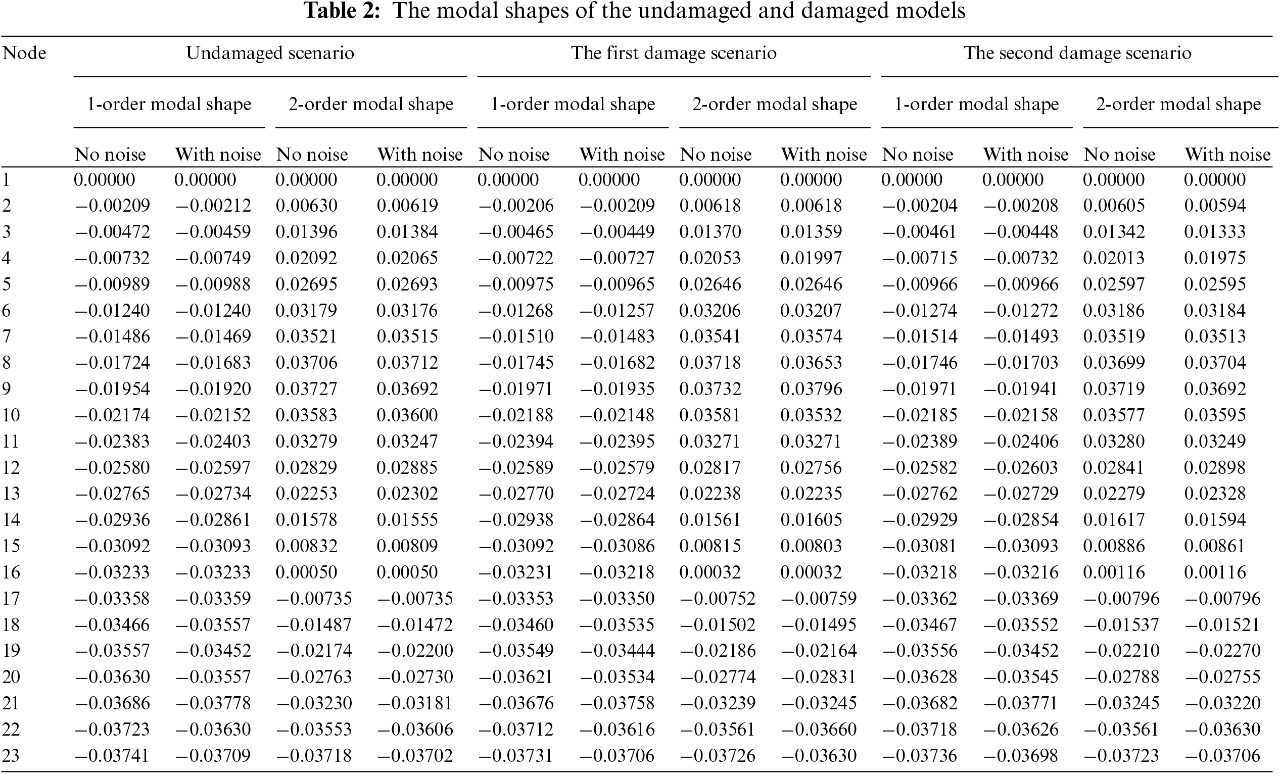
The proposed approach is validated again using the experiment data measured by Li from a three-story steel frame structure in reference [34]. The experimental structure, material parameters, and experimental process are described in detail in reference [34]. Fig. 6 provides the geometric model of this steel frame structure. From Fig. 6a, this structure is composed of three steel plates and four rectangular columns. These components are welded to simplify to a rigid shear system of Fig. 6b. The node numbers from bottom to top of this shear structure are 1, 2, 3, and 4. From vibration testing, the first natural frequency and modal shape of the undamaged structure are f1 = 3.369 and φ1 = (0.02118, 0.03922, 0.048427)T. The second modal data of the undamaged structure are f2 = 9.704 and φ2 = (0.048758, 0.02031, −0.03923)T. The third modal data of the undamaged structure are f3 = 14.282 and φ3 = (0.037936, −0.04866, 0.022852)T. Note that the conversion formula between the natural frequency fr and the aforementioned angular frequency (i.e., eigenvalue λr) is as follows:

λr=(2πfr)2(44)

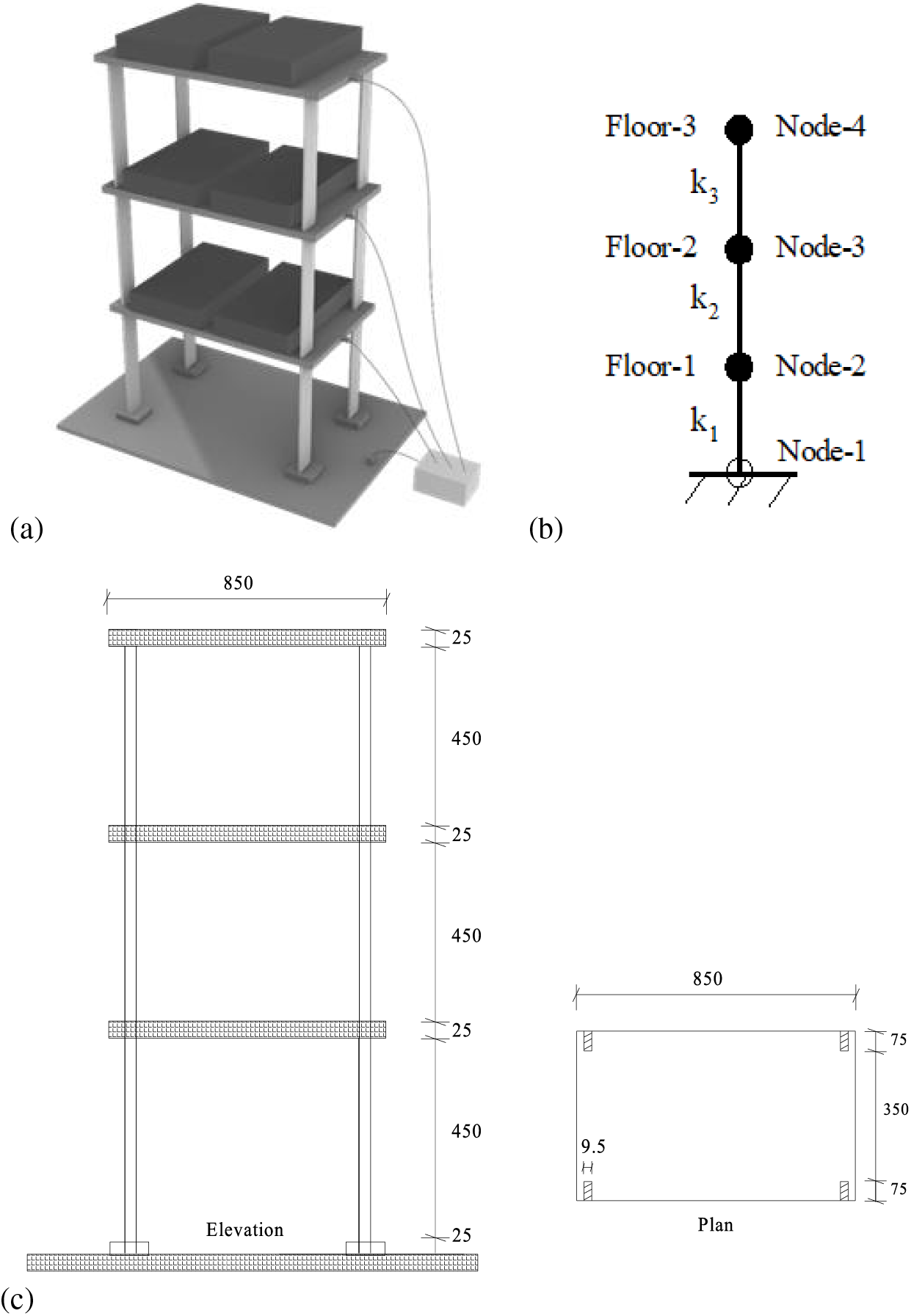
Figure 6: (a) A three-story experimental shear structure; (b) Simplified shear system corresponding to the experimental structure; (c) Geometric size of the experimental structure

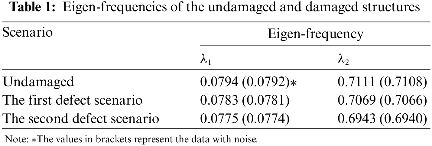
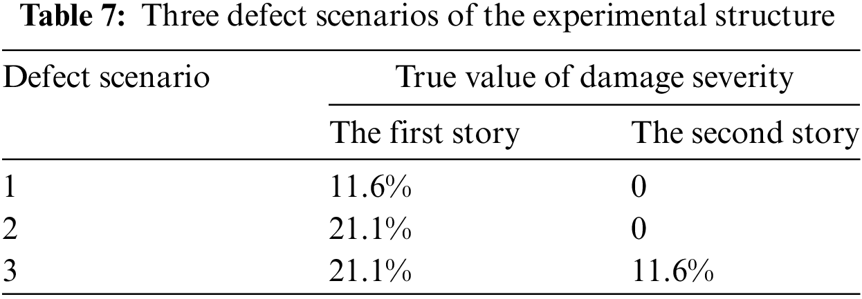
Some defect scenarios have been tested on this three-story steel frame structure in reference [34]. For the first defect scenario, the cross-sectional width of the lower ends of the four columns for the first floor has been reduced from 75 to 51.3 mm by cutting, as shown in Fig. 7a. The geometric dimensions before and after cutting are used to calculate the shear stiffness of the structure. The formula for calculating the shear stiffness was given in [34]. The ratio between the shear stiffness difference before and after cutting and the shear stiffness of the intact structure is used as the true value of the damage severity. For the first defect scenario, the true value of damage severity calculated based on the shear stiffness is 11.6%. For the second defect scenario, the cross-sectional width of the lower ends of the four columns for the first floor has been cut from 75 to 37.46 mm as shown in Fig. 7b. The corresponding true value of damage severity calculated based on the shear stiffness is 21.1%. The third damage scenario is to reduce the cross-sectional width of all column bottoms in the first floor from 75 to 37.46 mm, and to reduce the cross-sectional width of all column bottoms in the second floor from 75 to 51.3 mm, resulting in a damage degree of 21% and 11% for the first and second floors, respectively. These three defect scenarios are listed in Table 7.

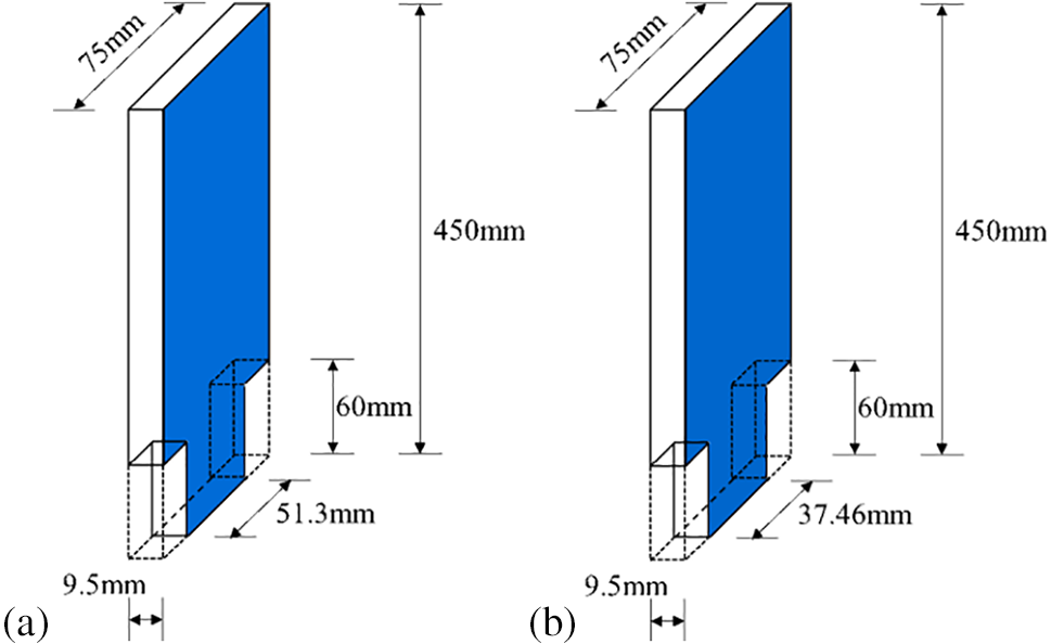
Figure 7: (a) Cut the width of the column bottom from 75 to 51.3 mm; (b) Cut the width of the column bottom from 75 to 37.46 mm

For the first defect scenario, the measured first-order modal data are fd1 = 3.259 and φd1 = (0.022735, 0.039331, 0.047594)T. The second-order modal data are fd2 = 9.485 and φd2 = (0.049417, 0.017683, −0.03968)T. The third-order modal data are fd3 = 14.209 and φd3 = (0.035798, −0.04982, 0.02379)T. Using only the first vibration mode, the specific process of calculating the damage localization vector Δξ using the proposed method is as follows:

(1) Calculate the undamaged flexibility matrix using Eq. (13) as:

F≈1λ1φ1φ1T=1(2πf1)2φ1φ1T=[0.09940.18480.22810.18480.34330.42390.22810.42390.5234]×10−5(45)

(2) Calculate the damaged flexibility matrix using Eq. (17) as:

Fd≈1λd1φd1φd1T=1(2πfd1)2φd1φd1T=[0.12330.21330.25810.21330.36890.44640.25810.44640.5402]×10−5(46)

(3) Calculate the change of flexibility matrix as:

ΔF=Fd−F=[0.23840.28500.29930.28500.25640.22560.29930.22560.1685]×10−6(47)

(4) Calculate damage localization vector Δξ using Eq. (21) with lv=(0,0,1)T as:

Δξ=ΔF⋅lv=[0.23840.28500.29930.28500.25640.22560.29930.22560.1685]×10−6×[001]=[0.29930.22560.1685]×10−6(48)

For convenience, Table 8 gives the calculation results of the defect localization vector Δξ shown in Eq. (48). Note in Table 8 that the node number is different from the floor number as shown in Fig. 6b. The node 1 in Table 8 corresponds to the fixed end of the structure. Obviously, the displacement difference before and after damage under any load is always zero at this fixed end position. Thus the value corresponding to node 1 is 0 in Table 8. From Table 8, one can find that there is a largest mutation between the nodes numbered 1 and 2, which exactly corresponds to the first floor. This means that the first floor is where the defect is most possibly located. For more accurate damage diagnosis, the fault coefficients for all floors can be computed by using the measured three frequencies with Eq. (40). The specific process of calculating the fault coefficients using the proposed method is as follows:

(1) Calculate the changes of the eigenvalues using Eq. (30) as:

[Δλ1Δλ2Δλ3]=[λd1−λ1λd2−λ2λd3−λ3]=[−28.7829−165.9037−82.1089](49)

(2) Calculate the eigenvalue sensitivity matrix S using Eqs. (29) and (39) as:

S=[∂λ1∂ε1∂λ1∂ε2∂λ1∂ε3∂λ2∂ε1∂λ2∂ε2∂λ2∂ε3∂λ3∂ε1∂λ3∂ε2∂λ3∂ε3]=[φ1TK1φ1φ1TK2φ1φ1TK3φ1φ2TK1φ2φ2TK2φ2φ2TK3φ2φ3TK1φ3φ3TK2φ3φ3TK3φ3]=[0.25150.18520.04791.34210.45692.00130.81244.23332.8870]×103(50)

(3) Calculate the fault coefficients using Eq. (40) as:

{ε1ε2ε3}=S+[Δλ1Δλ2Δλ3]=[−0.11850.0068−0.0050](51)

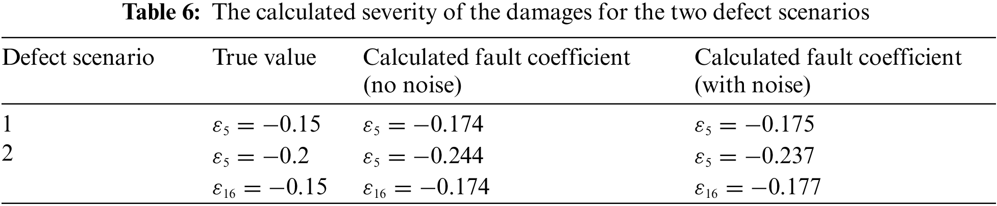
From Eq. (51), the calculated values of the fault coefficients are ε1=−0.1185, ε2=0.0068, and ε3=−0.0050, respectively. Based on these calculated damage severity values, it can be clearly determined that the first floor is damaged, while the second and third floors are not damaged since their calculated damage levels are very close to zero. The calculated damage severity value of the first floor (11.85%) is very close to the true value (11.6%). This indicates that the proposed method can successfully determine the location and severity of the defect in the experimental steel shear structure.

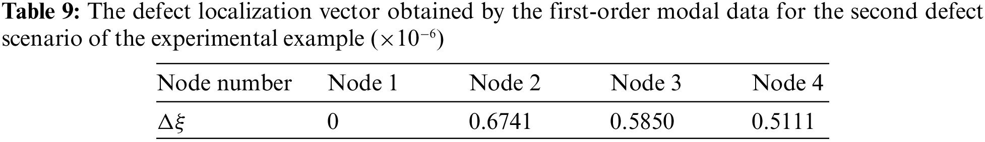
For the second defect scenario, the measured first-order modal data are fd1 = 3.113 and φd1 = (0.024117, 0.039364, 0.046881)T. The second-order modal data are fd2 = 9.302 and φd2 = (0.049711, 0.016267, −0.03992)T. The third-order modal data are fd3 = 14.136 and φd3 = (0.035067, −0.05014, 0.024199)T. Using only the first vibration mode, the damage localization vector Δξ obtained by the proposed method is given in Table 9. From Table 9, one can find that there is a largest mutation between the nodes numbered 1 and 2, which exactly corresponds to the first floor. This means that the first floor is where the defect is most possibly located. For more accurate damage diagnosis, the fault coefficients for all floors can be computed by the proposed method as: ε1=−0.2608, ε2=−0.0061, and ε3=0.0256, respectively. Based on these calculated damage severity values, it can be clearly determined that the first floor is damaged, while the second and third floors are not damaged since their calculated damage levels are very close to zero. The calculated damage severity value of the first floor (26.08%) is close to the true value (21.1%). This indicates that the proposed method can successfully determine the location and severity of the defect in the experimental steel shear structure.

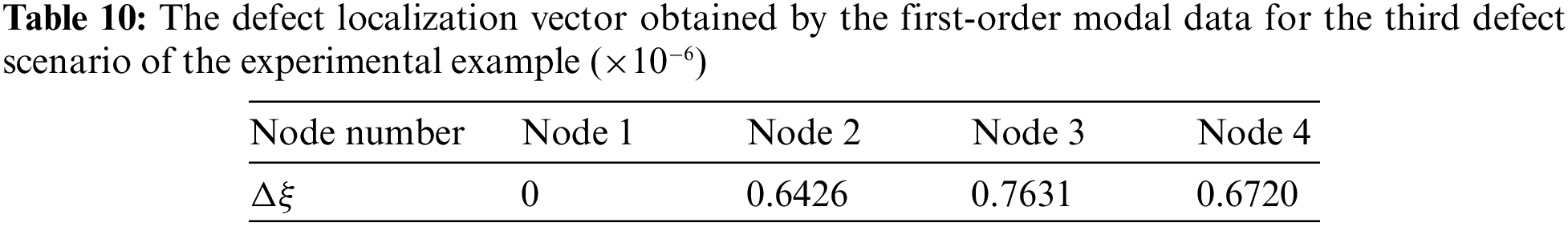
For the third defect scenario, the measured first-order modal data are fd1 = 3.076 and φd1 = (0.023253, 0.039779, 0.046968)T. The second-order modal data are fd2 = 9.192 and φd2 = (0.051655, 0.014387, −0.03813)T. The third-order modal data are fd3 = 13.660 and φd3 = (0.032448, −0.05058, 0.026788)T. Using only the first vibration mode, the damage localization vector Δξ obtained by the proposed method is given in Table 10. From Table 10, it can be observed that there is a large mutation between nodes 1 and 2, and a small mutation between nodes 2 and 3, which correspond to the first and second floors, respectively. This means that the first and second floors are where the defects are most possibly located. Note that the number of floors in this structure is only three, so the mutation feature is not as obvious as those structures with many floors. For more accurate damage diagnosis, the fault coefficients can be further computed by the proposed method as: ε1=−0.2145, ε2=−0.1053, and ε3=−0.0230, respectively. Based on these calculated fault coefficients, it can be clearly determined that the first and second floors are damaged, while the third floor is not damaged since its calculated damage level is close to zero. The calculated damage severity values of the first and second floors (21.45% and 10.53%) are close to the true values (21.1% and 11.6%). This indicates that the proposed method can successfully identify the location and severity of multiple defects in the structure.

5  Conclusions

In this paper, a new method of defect localization and quantitative evaluation is developed for the diagnosis of shear-type structural defects. The greatest advantage of the proposed method is that only a few low-frequency vibration modes of the shear structure need to be measured for defect diagnosis, without requiring a FEM of the structure. The proposed method completes the task of damage diagnosis through the first stage of defect localization and the second stage of defect quantitative evaluation. The proposed method has been successfully verified on a numerical model and an experimental model. According to the computation results, some conclusions can be summarized as follows. (1) For the numerical example, the location and severity of defects in the shear structure can be correctly diagnosed using only the first two vibration modal data. The proposed method can successfully identify defects in the structure even under the interference of 3% level noise. (2) For the experimental example, the most obvious mutation location in the damage location vector also corresponds to the location of the defect in the shear structure. The improved frequency sensitivity method can further accurately diagnose the damage in the shear structure and obtain the severity of the damage. (3) The method proposed in this paper does not require an overall FEM of the structure and complex mathematical operations during implementation, so it is particularly suitable for engineering applications. It has been shown that the proposed method may be very effective for defect diagnosis of shear-type structures.

Acknowledgement: None.

Funding Statement: This work is supported by the Zhejiang Public Welfare Technology Application Research Project (LGF22E080021), Ningbo Natural Science Foundation Project (202003N4169), Natural Science Foundation of China (11202138, 52008215), the Natural Science Foundation of Zhejiang Province, China (LQ20E080013), and the Major Special Science and Technology Project (2019B10076) of “Ningbo Science and Technology Innovation 2025”.

Author Contributions: The authors confirm contribution to the paper as follows: study conception and design: C.L., Q.Y.; data collection: Q.Y., X.P.; analysis and interpretation of results: C.L., Q.Y.; draft manuscript preparation: C.L., Q.Y., X.P. All authors reviewed the results and approved the final version of the manuscript.

Availability of Data and Materials: The data used to support the findings of this study are included within the article and also available from the corresponding author upon request.

Conflicts of Interest: The authors declare that they have no conflicts of interest to report regarding the present study.

References

1. Zhao, L., Shenton III, H. W. (2005). Structural damage detection using best approximated dead load redistribution. Structural Health Monitoring, 4(4), 319–339. [Google Scholar]

2. Abdo, M. A. B. (2012). Parametric study of using only static response in structural damage detection. Engineering Structures, 34, 124–131. [Google Scholar]

3. Avci, O., Abdeljaber, O., Kiranyaz, S., Hussein, M., Gabbouj, M. et al. (2021). A review of vibration-based damage detection in civil structures: From traditional methods to Machine Learning and Deep Learning applications. Mechanical Systems and Signal Processing, 147, 107077. [Google Scholar]

4. Ahmadi-Nedushan, B., Fathnejat, H. (2022). A modified teaching-learning optimization algorithm for structural damage detection using a novel damage index based on modal flexibility and strain energy under environmental variations. Engineering with Computers, 38(1), 847–874. [Google Scholar]

5. Yang, Q. W. (2019). Fast and exact algorithm for structural static reanalysis based on flexibility disassembly perturbation. AIAA Journal, 57(8), 3599–3607. [Google Scholar]

6. Yang, Q. W., Peng, X. (2023). A fast calculation method for sensitivity analysis using matrix decomposition technique. Axioms, 12(2), 179. [Google Scholar]

7. Peng, X., Yang, Q. W. (2022). Damage detection in beam-like structures using static shear energy redistribution. Frontiers of Structural and Civil Engineering, 16(12), 1552–1564. [Google Scholar]

8. Li, G. Q., Hao, K. C., Lu, Y., Chen, S. W. (1999). A flexibility approach for damage identification of cantilever-type structures with bending and shear deformation. Computers & Structures, 73(6), 565–572. [Google Scholar]

9. Koo, K. Y., Sung, S. H., Jung, H. J. (2011). Damage quantification of shear buildings using deflections obtained by modal flexibility. Smart Materials and Structures, 20(4), 045010. [Google Scholar]

10. Zhu, H., Li, L., He, X. Q. (2011). Damage detection method for shear buildings using the changes in the first mode shape slopes. Computers & Structures, 89(9–10), 733–743. [Google Scholar]

11. Xing, Z., Mita, A. (2012). A substructure approach to local damage detection of shear structure. Structural Control and Health Monitoring, 19(2), 309–318. [Google Scholar]

12. Su, W. C., Huang, C. S., Hung, S. L., Chen, L. J., Lin, W. J. (2012). Locating damaged storeys in a shear building based on its sub-structural natural frequencies. Engineering Structures, 39, 126–138. [Google Scholar]

13. Sung, S. H., Koo, K. Y., Jung, H. Y., Jung, H. J. (2012). Damage-induced deflection approach for damage localization and quantification of shear buildings: Validation on a full-scale shear building. Smart Materials and Structures, 21(11), 115013. [Google Scholar]

14. Panigrahi, S. K., Chakraverty, S., Mishra, B. K. (2013). Damage identification of multistory shear structure from sparse modal information. Journal of Computing in Civil Engineering, 27(1), 1–9. [Google Scholar]

15. Li, H., Tao, D., Huang, Y., Bao, Y. (2013). A data-driven approach for seismic damage detection of shear-type building structures using the fractal dimension of time-frequency features. Structural Control and Health Monitoring, 20(9), 1191–1210. [Google Scholar]

16. An, Y., Spencer Jr, B. F., Ou, J. (2015). Real-time fast damage detection of shear structures with random base excitation. Measurement, 74, 92–102. [Google Scholar]

17. Wang, D., Xiang, W., Zeng, P., Zhu, H. (2015). Damage identification in shear-type structures using a proper orthogonal decomposition approach. Journal of Sound and Vibration, 355, 135–149. [Google Scholar]

18. Mei, L., Mita, A., Zhou, J. (2016). An improved substructural damage detection approach of shear structure based on ARMAX model residual. Structural Control and Health Monitoring, 23(2), 218–236. [Google Scholar]

19. Luo, J., Liu, G., Huang, Z. (2017). Damage detection for shear structures based on wavelet spectral transmissibility matrices under nonstationary stochastic excitation. Structural Control and Health Monitoring, 24(1), e1862. [Google Scholar]

20. Shi, J. Y., Spencer Jr, B. F., Chen, S. S. (2018). Damage detection in shear buildings using different estimated curvature. Structural Control and Health Monitoring, 25(1), e2050. [Google Scholar]

21. Mei, L., Li, H., Zhou, Y., Wang, W., Xing, F. (2019). Substructural damage detection in shear structures via ARMAX model and optimal subpattern assignment distance. Engineering Structures, 191, 625–639. [Google Scholar]

22. Paral, A., Singha Roy, D. K., Samanta, A. K. (2019). Application of a mode shape derivative-based damage index in artificial neural network for structural damage identification in shear frame building. Journal of Civil Structural Health Monitoring, 9, 411–423. [Google Scholar]

23. Liang, Y., Feng, Q., Li, H., Jiang, J. (2019). Damage detection of shear buildings using frequency-change-ratio and model updating algorithm. Smart Structures and Systems, An International Journal, 23(2), 107–122. [Google Scholar]

24. Ghannadi, P., Kourehli, S. S. (2019). Model updating and damage detection in multi-story shear frames using Salp Swarm Algorithm. Earthquakes and Structures, 17(1), 63–73. [Google Scholar]

25. Do, N. T., Gül, M. (2020). A time series based damage detection method for obtaining separate mass and stiffness damage features of shear-type structures. Engineering Structures, 208, 109914. [Google Scholar]

26. Zhao, L., Jin, D., Wang, H., Liu, C. (2020). Modal parameter identification of time-varying systems via wavelet-based frequency response function. Archive of Applied Mechanics, 90(11), 2529–2542. [Google Scholar]

27. Liu, C., Fang, D., Zhao, L. (2021). Reflection on earthquake damage of buildings in 2015 Nepal earthquake and seismic measures for post-earthquake reconstruction. Structures, 30, 647–658. [Google Scholar]

28. Niu, Z. (2021). Two-step structural damage detection method for shear frame structures using FRF and Neumann series expansion. Mechanical Systems and Signal Processing, 149, 107185. [Google Scholar]

29. Yang, Q. W., Peng, X. (2023). A highly efficient method for structural model reduction. International Journal for Numerical Methods in Engineering, 124(2), 513–533. [Google Scholar]

30. Yang, Q. W., Peng, X. (2021). Sensitivity analysis using a reduced finite element model for structural damage identification. Materials, 14(19), 5514. [Google Scholar] [PubMed]

31. Tan, Y., Chen, Y., Lu, Z. R., Wang, L. (2022). Model-calibration-free damage identification of shear structures by measurement changes correction and sparse regularization. Structures, 37, 255–266. [Google Scholar]

32. Roy, K. (2023). Structural damage quantification in shear buildings using mode shape slope ratio. Structural Health Monitoring, 22(4), 2346–2359. [Google Scholar]

33. Yang, Q. W., Du, S. G., Liang, C. F., Yang, L. (2014). A universal model-independent algorithm for structural damage localization. Computer Modeling in Engineering & Sciences, 100, 223–248. https://doi.org/10.3970/cmes.2014.100.223 [Google Scholar] [CrossRef]

34. Li, L. (2005). Numerical and experimental studies of damage detection for shear buildings (Ph.D. Thesis). Huazhong University of Science and Technology, Wuhan, China. [Google Scholar]