Enriched Constant Elements in the Boundary Element Method for Solving 2D Acoustic Problems at Higher Frequencies

1  Introduction

The finite element method (FEM) [1] and the boundary element method (BEM) [2] are the two most popular methods for modeling the propagation of acoustic wave problems. In the FEM, the entire problem domain needs to be divided into area or volume for 2D or 3D elements, respectively. When an infinite domain is considered, a considerable number of finite elements are needed to solve the problem, or an artificial outer boundary needs to be introduced to transform the infinite domain into a bounded domain [3]. On the other hand, the BEM requires meshing only on the boundary [4] and can satisfy boundary conditions at infinity naturally. However, the coefficient matrix in the BEM is usually a dense and nonsymmetrical matrix, which can lead to a much larger storage requirement and more computing time to solve the BEM equations compared with other methods.

Researchers have developed numerous techniques in the last few decades to improve the efficiency of the BEM solutions, including the fast multipole method for potential, elastostatic, and acoustic problems (see some works in [5–11]), adaptive cross approximation method (e.g., [12–15]), and fast direct solver method (e.g., [16–19]). These methods all aim to speed up the solutions of the BEM equations and have already achieved significant progress. However, some researchers have also considered further reducing the dimensionality of the problem domain (including the 2.5D singular boundary method [20]) or improving the quality of the representation of boundary variables in the BEM to reduce the BEM model size.

Using enriched elements is one way to reduce the size of the BEM matrix while maintaining the accuracy of the model. One of the methods used to enrich elements is the partition-of-unity method (PUM). The PUM was proposed by Melenk et al. in 1996 [21] and initially used in the FEM [22–25]. The basic idea of the PUM is to apply new functions to enrich or expand the solution space and enable accurate solutions with a coarse mesh, while the use of original polynomials in the conventional finite elements ensures convergence when the mesh is refined. With the aid of the PUM, the simulation of problems with singularities (e.g., crack propagation [26,27]) and acoustic wave propagation [28,29] becomes much easier. In the BEM literature, Trevelyan et al. have published some interesting and promising work on coupling the BEM with the PUM [30–34] and using plane wave interpolation. The majority of their studies, however, have focused on using higher-order elements (quadratic or isogeometric elements) to represent the geometries of the domain accurately, while the enriched terms have been applied to represent the field more accurately and thus significant reductions in the number of elements in a BEM model can be achieved.

In solving acoustic problems, however, the desired results of acoustic quantities are often at locations far away from the boundary of the domain. The use of higher-order elements may not be critical. Therefore, constant boundary elements are often applied in the acoustic BEM because they are easier to implement (regarding the treatment of corner problems and analytical integration of the singular integrals). They are often used with fast solution methods for the acoustic BEM owing to these advantages [9]. However, the accuracy of using constant elements is often poorer than using high-order elements. It is thus worthwhile and intriguing to study the enriched constant elements, which has not been done, to improve the accuracy of using the constant elements in the acoustic BEM.

In this study, we propose two types of enrichment constant elements in the BEM for 2D acoustic wave problems: 1) a plane wave expansion with constant elements, for modeling scattering problems; and 2) a special plane wave expansion with constant elements, for solving radiation problems. Two verification problems are used to study the performance of the proposed elements regarding computational efficiency and accuracy. The numerical results show that enriched constant elements perform well in both scattering and radiation problems and that using even a single-term expansion can reduce errors markedly. The plane-wave-expansion elements are also used in solving two larger-scale problems and an acoustic meta-material model. The proposed work is novel in that it uses the enriched element concept with constant elements for the acoustic BEM. The enriched constant elements are easy to implement, more accurate, and more efficient compared with the regular constant elements.

The rest of this paper is organized as follows: In Section 2, we introduce the BEM and the enriched elements. In Section 3, two numerical verification cases using the enriched elements are presented. In Section 4, three application cases are tested, and details of the models and results are discussed. In Section 5, discussions on the potential, improvements, and future work with enriched constant elements are presented to conclude the paper.

2  Constant and Enriched Elements for 2D Acoustic BEM

2.1 Boundary Integral Equation

Consider the propagation of time-harmonic acoustic waves in a homogeneous isotropic acoustic medium Ω (either finite or infinite), governed by the following Helmholtz equation (e.g., Chapter 6 in [9]):

∇2ϕ(x)+k2ϕ(x)=0,∀x∈Ω,(1)

where ∇2 is the Laplacian operator, ϕ(x) is the acoustic pressure at point x, k=ω/c is the wave number, ω is the angular frequency, and c is the sound speed.

The boundary conditions for acoustic problems can be the Dirichlet boundary condition, Neumann boundary condition, or Robin boundary condition. For exterior domain problems, the Sommerfeld condition at infinity must also be satisfied.

Using Green’s second identity, and letting point x approach the boundary, we can obtain the boundary integral equation (BIE) as follows [9]:

c(x)ϕ(x)=∫S[G(x,y,ω)q(y)−F(x,y,ω)ϕ(y)]dS(y)+ϕI(x),(2)

where c(x)=1/2 for source point x on the boundary S (assumed to be smooth), y is the integration point on the boundary, q(y) is the normal derivative of the sound pressure at point y, and ϕI(x) is the incident wave and does not present in a pure radiation problem. The fundamental solution G(x,y,ω) and the normal derivative of the fundamental solution F(x,y,ω) for 2D acoustic problems are given by:

G(x,y,ω)=i4H0(1)(kr),F(x,y,ω)=∂G(x,y,ω)∂n(y)=−ik4H1(1)(kr)r,lnl(y),(3)

where Hn(1)() represents the Hankel function of the first kind, i=−1 is the imaginary unit number, and r is the distance between points x and y.

In the BEM, the boundary can be discretized using constant, linear, quadratic, or other higher-order elements. For solving acoustic problems, we use the constant elements to yield the following discretized form of the BIE (BEM equations) [9]:

12ϕ(x)+∑j=1N∫SjF(x,y,ω)ϕjdS(y)=∑j=1N∫SjG(x,y,ω)qjdS(y)+ϕI(x),(4)

where N is the number of elements; Sj is the jth element on boundary S, which is divided into a total number of N elements; and ϕj and qj are the constant acoustic pressure and normal derivative of the pressure on element Sj, respectively.

We collocate x at the midpoint of each element and rearrange the equations into a standard linear system of equations after applying the boundary conditions to solve Eq. (4) using constant elements:

Aλ=b,(5)

where A is the coefficient matrix with a dimension of N by N, λ is the unknown vector with unknown ϕj or qj on each element, and b is the known right-hand side vector computed from the known boundary values and/or incident wave.

2.2 Enriched Element

To introduce the enrichment, we use a new function on a constant element to better represent the acoustic field on the element. For example, for scattering problems, we describe the sound pressure on the element as the sum of a series of plane waves as follows (instead of assuming it is constant on the element):

ϕ(y)=∑l=1LAleikdl⋅y,(6)

where L is the number of plane waves used, and Al is the amplitude of the pressure at point y for the plane wave in direction dl. The unit directional vector dl can be expressed as follows:

dl=(cos⁡θl,sin⁡θl),(7)

where θl is the angle one can choose, such as

θl=2π(l−1)L+θI,l=1,2,…,L,(8)

where θI is the angle of the incident plane wave with respect to the x-axis. For scattering from a hard surface, we have q=0 on the boundary, and the discretized form of the BIE (Eq. (4)) using the plane-wave-enriched constant elements can be written as follows:

12ϕ(x)+∑j=1N∑l=1L[∫SjF(x,y,ω)eikdl⋅ydS(y)]Alj=ϕI(x),(9)

where Alj is the unknown amplitude of direction dl on the jth element.

The integral on element Sj is computed using a Gaussian quadrature for nonsingular cases. For singular cases, the values of the integral vanish because of the term r,lnl(y)=0 in the F kernel. To provide a sufficient number of equations, we must also expand the term ϕ(x) on the left-hand side of Eq. (9) using Eq. (6).

For radiation problems, it is found that the use of plane wave expansions as in Eq. (6) does not perform as well as in the scattering case. Therefore, another special wave expansion is attempted, in which the acoustic pressure and its derivative on this enriched element are described as

ϕ(y)=Aeikξ(y),q(y)=Beikξ(y),(10)

where ξ(y) is the distance from a reference point to point y, which we select (the method of selecting ξ(y) is discussed later with examples); A and B are the amplitudes of the sound pressure and its normal derivative, respectively. Thus, the discretized BIE using the special plane wave expansion for constant elements for radiation problems can be written as follows:

12ϕ(x)+∑j=1N[∫SjF(x,y,ω)eikξ(y)dS(y)]Aj=∑j=1N[∫SjG(x,y,ω)eikξ(y)dS(y)]Bj.(11)

In Eq. (11), we use a Gaussian quadrature for both singular and nonsingular cases. On a singular element (a straight line in 2D), the integral of F(x,y,ω)eikξ(y) is zero, and the integral of G(x,y,ω)eikξ(y) is weakly singular. Both can be computed using the standard quadrature formula within an acceptable range of errors.

The unknowns on a traditional constant element, an enriched element for scattering problems, and an enriched element for radiation problems are shown in Fig. 1. Note that in the scattering problems, the unknown pressure ϕ in the enriched elements is replaced by the unknown amplitude Al in the direction dl, as Fig. 1b shows. In the radiation problems, the unknown pressure ϕ or its norm derivative q is replaced by the unknown amplitude A or B, which is along the direction of the vector from the pre-set point to the point y, as Fig. 1c shows. As a result, the number of DOFs in a mesh using constant element discretization is changed from the number of elements N to NL in scattering problems. To provide additional equations, we select L collocation points on each element for the enriched elements, compared to just one collocation point on each element in the conventional constant element case.

Figure 1: Unknowns on a constant element (a), an enriched element for scattering problems (b), and an enriched element for radiation problems (c)

Therefore, the linear system of the BEM equations with the enriched elements becomes

A′λ′=b′,(12)

where A′ is the coefficient matrix with a dimension of NL by NL (for the special wave expansion enriched element L = 1), λ′ is the unknown vector consistent with L new unknowns on each element, and b′ is the new known right-hand side vector computed with the given boundary values.

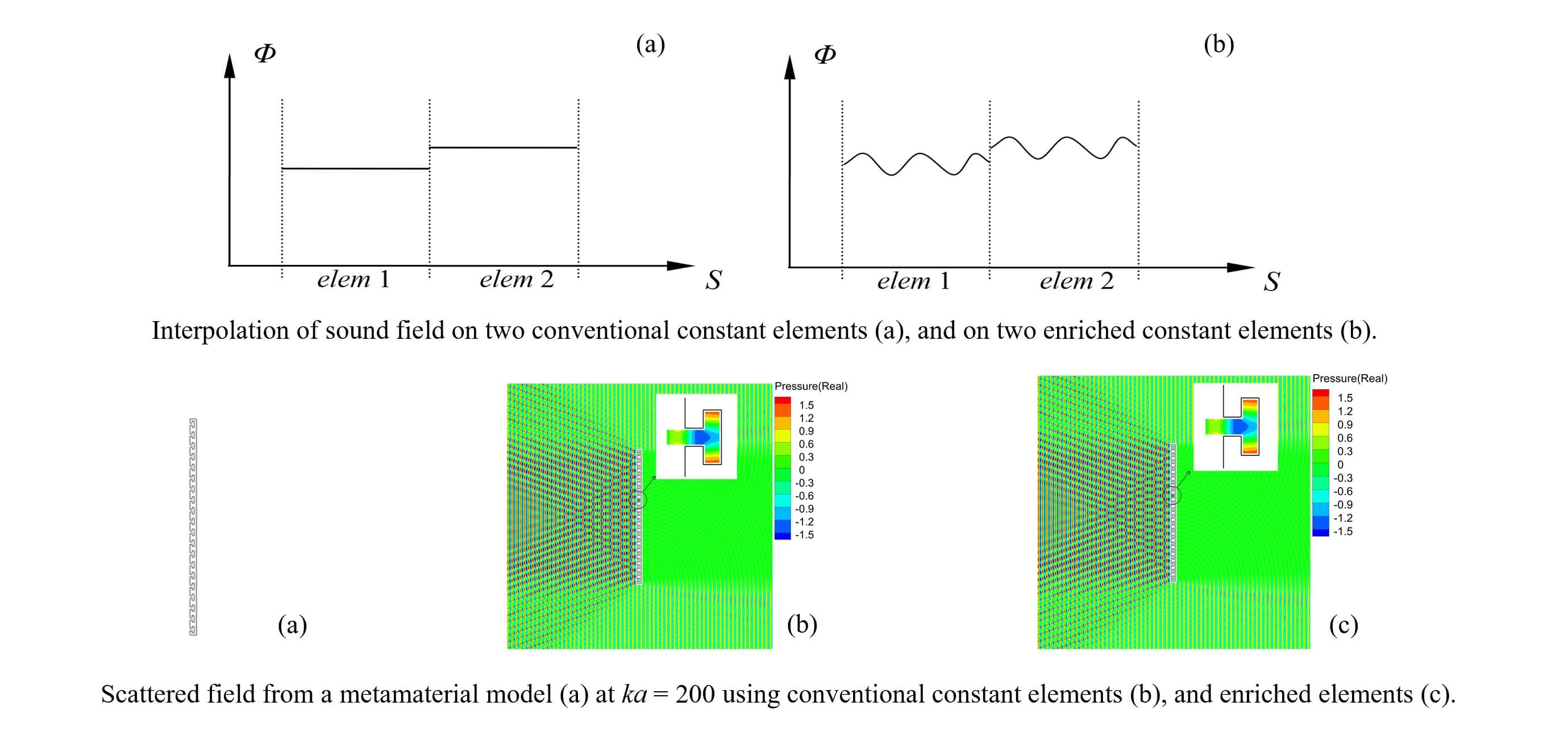
From Eqs. (4) and (9), we can observe that the sound pressures on the enriched elements are represented differently compared with the case using the conventional constant elements. The sound pressure on the enriched elements can have one or more wave shapes on a single element (Fig. 2), instead of having constant values on each entire element. Clearly, better results can be expected using the enriched elements as they can represent the wave shapes better than the conventional elements.

Figure 2: Illustration of the variations of sound pressure on two conventional constant elements (a) and on two enriched constant elements (b)

3  Verification Problems

We consider a problem with a circular scatterer (an infinitely long cylinder) and another problem with a pulsating cylinder, both in a 2D infinite domain, to verify the correctness of the enriched elements presented in the previous section. In both cases, the circular domain has a radius of 1 m and is discretized with 60 elements initially. A field surface is defined by a square region of 15 m × 15 m around the cylinder and is placed with 2,080 field points to measure the error of the calculation. We use the L2-norm to evaluate the error ε:

ε=‖Φ−Φex‖L2‖Φex‖L2,(13)

where Φ is the vector of sound pressure values at the field points calculated using either the conventional constant elements or the enriched constant elements, and Φex is the vector of sound pressure values evaluated using the analytical solution. All the computations are done on a desktop computer with an Intel® Xeon® CPU E5-2650 v4 and 64 GB of RAM.

3.1 Scattering Problem

The sound-hard boundary condition is considered for the problem of scattering from the cylinder, with an incident plane wave propagating in the +x direction. The total wave for this scattering problem can be calculated using the analytical solution [35]:

ϕex(x)=ϕI(x)−A0[J0′(k)H0′(1)(k)Hn(1)(kr)+2∑n=1∞inJn′(k)Hn′(1)(k)Hn(1)(kr)cos⁡nθ],(14)

where A0 is the amplitude of an incident plane wave, r and θ are the polar coordinates for point x, and Jn() is the Bessel function of the first kind of order n.

The results using the enriched elements with L = 1, 3, 5, 7 and the conventional constant elements are shown in Fig. 3, in which ka is the product of the wave number and the characteristic length (in this case, a = 2 m). We plot the results for sound pressure at point (5, 0) m, with (0, 0) m being the center of the cylinder and ka being between 2 and 100 at an interval of 2. The plot shows that the results obtained using the enriched elements with L = 1, 3, 5, 7 have a significantly higher degree of accuracy than those obtained using the conventional constant elements, with the increase in the frequencies up to ka = 100. It is observed that all tested enriched elements can deliver good results within a ka range of 1–100, a much wider range than that of using the conventional constant element. It is also noticed that the results at a few frequencies exhibit spikes with larger errors, which is the case of the fictitious eigenfrequency difficulty for exterior domain problems. This issue will be addressed in future work.

Figure 3: Results using conventional constant elements and plane-wave-enriched elements with L = 1, 3, 5, 7 at the field point (5, 0) m

The contour plots of the computed sound pressure distributions on the field surface using the analytical solution, conventional constant elements, and the enriched constant elements with L = 1 at ka = 50 are shown in Fig. 4. Clearly, the results agree well using the two types of elements. In this case, the memory and computational costs of using the plane-wave-enriched elements are nearly identical to those using the conventional constant element.

Figure 4: Contour plots of the computed sound pressure at ka = 50 on the field surface using the analytical solution (a), conventional constant elements (b), and enriched constant elements with L = 1 (c)

An enriched constant element with three expansion terms has the same number of DOFs as that of three conventional constant elements. Therefore, we next compare the results for the scattering cylinder using these two types of elements with the same number of DOFs.

The computing time for the two types of elements with the same number of DOFs is shown in Table 1, in which ka refers to the wave number before the first occurrence of error greater than 5%, and the time is the duration it takes to calculate all the 2,080 field points from k = 1 to k = 100 at an interval of 1, for a total of 100 calculations. We notice that for the same number of DOFs, the enriched elements take less time than the conventional constant elements. As the number of elements increases, the time reduction using the enriched elements also increases.

The errors when using 420 conventional constant elements and 60 enriched constant elements with seven expansion terms (number of DOFs = 60 × 7 = 420) are shown in Fig. 5. With the same number of DOFs, the results calculated using these two types of elements show no significant difference in the results. However, the calculation time is lower when using the enriched elements than when using conventional constant elements (see the last row of Table 1).

Figure 5: Comparison of 420 conventional elements and 60 enriched elements with L = 7 at point (5, 0) m

3.2 Radiation Problem

Next, the model of a pulsating cylinder (with a radius of 1 m) is considered, with a constant pressure boundary condition (ϕ=100+0i) prescribed. The analytical solution for this radiation problem is given by the following equation [35]:

ϕ(x)=ϕ0H0(1)(kr),(15)

where ϕ0 is the amplitude of the sound pressure. Consider the radiation problem for ka in the range of 2–116 at intervals of 2.

We first test the case using the same type of plane-wave-expansion-enriched constant elements as used for the scattering problem. The errors of the results are shown in Fig. 6. In this test, the results of the enriched elements with L = 1, 3, 5 are calculated. By setting 5% as the upper limit of errors, we find that the constant elements perform well when ka < 80, while the results using the plane-wave-enriched elements with L = 1, 3 are unsatisfactory. This is because radiation waves have different directions as the normal direction of the boundary changes. For the radiation problem, the waves propagate mainly along the normal direction near the boundary. However, in the plane wave expansion, the direction we set does not coincide with the normal direction of the elements, which can lead to errors. The error decreases as the number of expansion terms increases to L = 5, as shown in Fig. 6. This is because with the increase in the expansion terms, one of the directions in the expansions is more likely to be closer to the normal direction of the boundary.

Figure 6: Errors in conventional constant elements and plane-wave-enriched elements with L = 1, 3, 5

Based on this observation, to more effectively model the radiation problems with the enriched elements, we turn to the special plane-wave-expansion-enriched constant elements, as introduced in Eq. (10). In this example, the parameter ξ is chosen as the radius of the cylinder, which leads to a constant density function on each element (see Eq. (10)). However, this constant has a plane wave component and is not an arbitrary constant, as in the case of the conventional constant element. With this enriched element, we calculate ka in the range of 2–110, and the errors for using conventional constant elements and enriched constant elements are shown in Fig. 7. Compared with the results in Fig. 6, we can see that the special plane-wave-expansion-enriched elements have a better accuracy than the plane-wave-expansion element with L = 1, 3. Therefore, the targeted special plane-wave-enriched element is more efficient for modeling radiation problems than just using the same plane wave expansions as used for the scattering problems, and with more terms.

Figure 7: Errors in results using conventional constant elements and the special plane-wave-enriched elements for the radiation problem

The contour plots of the computed sound pressure on the field surface at ka = 42 using the analytical solution, conventional constant elements, and enriched elements with the special plane wave expansion are shown in Fig. 8. Good agreement is observed among these three plots.

Figure 8: Contour plots of the computed sound pressure on the field surface at ka = 42 using analytical solution (a), conventional constant elements (b), and enriched elements with special plane wave expansion (c)

4  Application Examples

In this section, to verify the effectiveness and efficiency of using the proposed enriched elements, we consider models of three problems on domains with more complicated geometries. To verify the accuracy of the enriched elements, we use the L2-norm in Eq. (13), in which Φex is evaluated using the converged solutions with the conventional constant elements. In all subsequent scattering cases, unless otherwise specified, we use 20 Gaussian integration points for the boundary integrals and five Gaussian integration points for the calculations at the field points.

4.1 Scattering from Multiple Cylinders

First, we study the scattering problem from a regular array of 25 (5 × 5) infinitely long circular cylinders. To describe the geometry and field accurately in this case, we use a large number of plane-wave-enriched elements. This model is used to verify whether the enriched elements are suitable for solving larger-scale BEM models.

For scattering from a hard surface, the boundary condition is q = 0. The incident plane wave propagates in the +x direction. Each cylinder has a radius of 1 m, and the distance between the centers of two neighboring cylinders is 3 m. We test this case with k = 45 1/m, and the overall nondimensional wave number ka value reaches 630 in this case. Each cylinder is divided into 1,750 conventional constant elements for obtaining the converged results, with a total of 43,750 conventional constant elements used in the entire model. When the plane-wave-expansion-enriched elements are used, we only need 400 elements for each cylinder, so there are only 10,000 elements in the entire model. A field surface is defined by a square region of 16 m × 16 m around the model to calculate the acoustic pressure and error on this surface.

The contour plots of the sound pressure on the field surface with different numbers of plane-wave-expansion terms are shown in Fig. 9. There is no significant difference in the contour plots with different numbers of expansion terms, as shown in the figure.

Figure 9: Contour plots of sound pressure for multiple cylinders computed using conventional and enriched elements using expansions with different numbers of terms

The comparison of the numbers of elements, total numbers of DOFs, percent differences in the solutions, and computing times when using the two methods is shown in Table 2. The first row of the table shows the results using the conventional constant elements, and the following rows show the results using the enriched elements. It can be seen from the data in Table 2 that the enriched elements can be used in solving larger models, with significantly reduced computational time.

4.2 Radiation of Multiple Cylinders

In this case, to calculate a radiation problem and investigate the effectiveness of the special plane-wave-enriched elements, we use the same model as in the previous section. For this purpose, the number of elements for each circle is set to 300 in the current calculations, which is sufficient for obtaining converged results using the conventional constant elements for the radiation problem when k = 15 1/m. The boundary condition for this radiation problem is set as q = 1. The parameter ξ is chosen as the radius of the cylinder, as in the single-cylinder radiation case.

The contour plots of sound pressure computed for the model with multiple cylinders at k = 15 1/m using the conventional constant elements and special plane-wave-enriched elements are shown in Fig. 10. From the contour plots, it is observed that results obtained using the two types of elements are in good agreement. The L2-norm is also calculated regarding the difference between the two solutions. It is found that the difference between the results using the two types of elements is only 3.87%. This suggests that the special plane-wave-enriched elements can deliver accurate results in modeling larger radiation problems.

Figure 10: Contour plots for multiple cylinders at k = 15 1/m using conventional constant elements (a) and special plane-wave-enriched elements (b)

4.3 Meta-Material Model

In this case, we study the scattering problem of an acoustic meta-material model using the enriched elements to demonstrate the feasibility of the enriched elements in solving problems in domains with complex geometries. The rule for selecting angles of the expansion terms for the enriched elements in this case is related not only to the incidence angle of the plane wave but also to the direction normal to the boundary. We choose the first angle θ1=θI, and the rest of the angles can be expressed as follows:

θl=θn−π2+(l−1)Lπ,l=2,3,4,…,L,(16)

in which θn is the direction normal to the element.

The structure of the meta-material model is shown in Fig. 11, which is a long rectangle with dimensions of 0.03 m × 1 m. For each unit cell in this periodic structure, the sizes can be designed according to the targeted frequency. In this case, the specific dimensions are marked in Fig. 11b. This model is studied with an incident plane wave traveling from left to right and with k = 200 1/m, and the sound-hard boundary condition is considered. The field surface is defined by a square region of 2 m × 2 m around the model to calculate the sound pressure and error (differences) on this surface.

Figure 11: A meta-material model used in the scattering problem

The contour plots of the acoustic wave propagation under the influence of structures in the meta-material model are shown in Fig. 12. The sound waves are focused in front of the meta-material model; behind the model, the sound waves are almost insulated. Although the sound pressure distributions near the model using the one-term enriched elements are not the same as those using the constant elements in the small channel areas (shown in the insets), the overall L2-norms of results between the conventional constant elements and enriched constant elements are found to be below 2% when three and five expansion terms are used in the enriched elements, as shown in Table 3.

Figure 12: Contour plots of results for the meta-material model at k = 200 1/m using conventional and enriched elements

In Table 3, the first row of numbers shows the results using 2,928 conventional constant elements. The remaining three rows show the results using the same mesh of 366 enriched elements with different numbers of expansion terms. It is shown that the enriched elements perform equally well in the model of meta-material as they do in the case of multiple cylinders. However, to obtain more accurate results when working with complex models, like those for meta-materials, more expansion terms are required. As observed in the previous example, using the enriched elements can reduce the computing time significantly, with the same level of accuracy.

Table 3 shows that for a fixed number of elements (366 elements), the accuracy of using the enriched elements improves as L increases. When we use the number of expansion terms L = 5, the accuracy of the result can converge with the difference below 0.5%, compared with that of the conventional constant elements. For numbers of expansion terms L = 1 and 3, differences in the results can also converge to below 1% if more elements are used, as shown in Table 4.

Based on the results in Tables 3 and 4, it is evident that using the enriched elements comes with a few advantages. Specifically, the number of DOFs can be reduced, and the computing time can be shortened compared with using the conventional constant elements. Furthermore, an increase in either the number of elements or the value of L can yield converged results. It is demonstrated that applying enriched elements can improve the computational accuracy of a mesh with a fixed number of elements. Thus, the meta-material model and results show that enriched elements can be used to solve larger-scale models with more complex geometries.

5  Discussion

In this paper, two types of enriched constant elements to solve 2D acoustic wave problems are proposed: 1) a plane wave expansion, for scattering problems, and 2) a special plane wave expansion for radiation problems. These new enriched elements can be applied to solve acoustic wave problems at higher frequencies as demonstrated by the verification and application cases. To verify the accuracy of these enriched elements, two verification cases have been studied. To show their capability to solve problems with more complex geometries, three application cases have been studied. It has shown that using the plane-wave-expansion-enriched constant elements is more efficient than using the conventional constant elements for solving scattering and radiation problems with the same number of DOFs. It has also shown that the error in the results is fewer when using the enriched elements than when using the conventional constant elements at the same frequency when a boundary mesh is given. Our work is novel in using enriched elements with constant elements, making it easy to implement in the treatment of corners of geometries and analytical integration of singular integrals.

The plane-wave-expansion-enriched elements and the special-plane-wave-expansion-enriched elements still need to be improved regarding their implementations and solutions of the BEM system of equations. The fictitious eigenfrequency problems existing with the conventional BIE need to be addressed. These enriched elements can also be extended to solve 3D acoustic wave problems, although the implementation will be more complicated. The solution of the BEM equations with the enriched boundary elements can be accelerated using the fast multipole method [9] or adaptive cross approximation methods [11,13]. All these are interesting topics for further research work.

Acknowledgement: The authors would like to thank the anonymous reviewers and journal editors for providing useful comments and suggestions.

Funding Statement: The authors would like to thank the following for their financial support for this work: the National Natural Science Foundation of China (https://www.nsfc.gov.cn/; Project No. 11972179), the Natural Science Foundation of Guangdong Province (http://gdstc.gd.gov.cn/; No. 2020A1515010685), and the Department of Education of Guangdong Province (http://edu.gd.gov.cn/; No. 2020ZDZX2008).

Author Contributions: The authors confirm contribution to the paper as follows: study conception and design: Zonglin Li, Yijun Liu; program and data collection: Zonglin Li; analysis and interpretation of results: Zonglin Li, Zhenyu Gao, Yijun Liu; draft manuscript preparation: Zonglin Li, Yijun Liu. All authors reviewed the results and approved the final version of the manuscript.

Availability of Data and Materials: None.

Conflicts of Interest: The authors declare that they have no conflicts of interest to report regarding the present study.

References

1. Zienkiewicz, O. C., Taylor, R. L., Zhu, J. Z. (2013). The finite element method: Its basis and fundamentals. Oxford: Butterworth-Heinemann. [Google Scholar]

2. Brebbia, C. A. (1978). The boundary element method for engineers. London: Pentech Press. [Google Scholar]

3. Babuška, I., Ihlenburg, F., Paik, E. T., Sauter, S. A. (1995). A generalized finite element method for solving the Helmholtz equation in two dimensions with minimal pollution. Computer Methods in Applied Mechanics and Engineering, 128(3), 325–359. [Google Scholar]

4. Liu, Y. J. (2019). On the BEM for acoustic wave problems. Engineering Analysis with Boundary Elements, 107, 53–62. [Google Scholar]

5. Greengard, L., Rokhlin, V. (1987). A fast algorithm for particle simulations. Journal of Computational Physics, 73(2), 325–348. [Google Scholar]

6. Peirce, A. P., Napier, J. A. L. (1995). A spectral multipole method for efficient solution of large-scale boundary element models in elastostatics. International Journal for Numerical Methods in Engineering, 38(23), 4009–4034. [Google Scholar]

7. Nishimura, N., Yoshida, E. I., Kobayashi, S. (1999). A fast multipole boundary integral equation method for crack problems in 3D. Engineering Analysis with Boundary Elements, 23(1), 97–105. [Google Scholar]

8. Shen, L., Liu, Y. J. (2007). An adaptive fast multipole boundary element method for three-dimensional acoustic wave problems based on the Burton-Miller formulation. Computational Mechanics, 40(3), 461–472. [Google Scholar]

9. Liu, Y. J. (2009). Fast multipole boundary element method: Theory and applications in engineering. Cambridge: Cambridge University Press. [Google Scholar]

10. Gumerov, N. A., Kaneko, S., Duraiswami, R. (2023). Recursive computation of the multipole expansions of layer potential integrals over simplices for efficient fast multipole accelerated boundary elements. Journal of Computational Physics, 486, 112118. [Google Scholar]

11. Zhang, Y., Liu, Y. J. (2023). Fast evaluations of integrals in the Ffowcs Williams-Hawkings formulation in aeroacoustics via the fast multipole method. Acoustics, 5(3), 817–844. [Google Scholar]

12. Hackbusch, W. (1999). A sparse matrix arithmetic based on ℋ-matrices. Part I: Introduction toℋ-matrices. Computing, 62(2), 89–108. [Google Scholar]

13. Bebendorf, M., Rjasanow, S. (2003). Adaptive low-rank approximation of collocation matrices. Computing, 70(1), 1–24. [Google Scholar]

14. Bebendorf, M. (2008). Hierarchical matrices: A means to efficiently solve elliptic boundary value problems. Heidelberg, Berlin: Springer-Verlag. [Google Scholar]

15. Brancati, A., Aliabadi, M. H., Benedetti, I. (2009). Hierarchical adaptive cross approximation GMRES technique for solution of acoustic problems using the boundary element method. Computer Modeling in Engineering & Sciences, 43(2), 149–172. https://doi.org/10.3970/cmes.2009.043.149 [Google Scholar] [CrossRef]

16. Martinsson, P. G., Rokhlin, V. (2005). A fast direct solver for boundary integral equations in two dimensions. Journal of Computational Physics, 205(1), 1–23. [Google Scholar]

17. Lai, J., Ambikasaran, S., Greengard, L. (2014). A fast direct solver for high frequency scattering from a large cavity in two dimensions. Siam Journal on Scientific Computing, 36(6), B881–B903. [Google Scholar]

18. Huang, S., Liu, Y. J. (2017). A new fast direct solver for the boundary element method. Computational Mechanics, 60(3), 379–392. [Google Scholar]

19. Li, R. Y., Liu, Y. J., Ye, W. J. (2023). A fast direct boundary element method for 3D acoustic problems based on hierarchical matrices. Engineering Analysis with Boundary Elements, 147, 171–180. [Google Scholar]

20. Wei, X., Luo, W. (2021). 2.5D singular boundary method for acoustic wave propagation. Applied Mathematics Letters, 112, 106760. [Google Scholar]

21. Melenk, J. M., Babuska, I. (1996). The partition of unity finite element method: Basic theory and applications. Computer Methods in Applied Mechanics and Engineering, 139(1–4), 289–314. [Google Scholar]

22. Taylor, R. L., Zienkiewicz, O. C., Oñate, E. (1998). A hierarchical finite element method based on the partition of unity. Computer Methods in Applied Mechanics and Engineering, 152(1), 73–84. [Google Scholar]

23. Babuška, I., Zhang, Z. (1998). The partition of unity method for the elastically supported beam. Computer Methods in Applied Mechanics and Engineering, 152(1), 1–18. [Google Scholar]

24. Dolbow, J., Moës, N., Belytschko, T. (2000). Discontinuous enrichment in finite elements with a partition of unity method. Finite Elements in Analysis and Design, 36(3), 235–260. [Google Scholar]

25. Hazard, L., Bouillard, P., Sener, J. Y. (2006). A partition of unity finite element method applied to the study of viscoelastic sandwich structures. III European Conference on Computational Mechanics, Dordrecht. [Google Scholar]

26. Moës, N., Sukumar, N., Moran, B., Belytschko, T. (2000). An extended finite element method (X-FEM) for two-and three-dimensional crack modeling. European Congress on Computational Methods in Applied Sciences and Engineering, Barcelona. [Google Scholar]

27. Gasser, T. C., Holzapfel, G. A. (2005). Modeling 3D crack propagation in unreinforced concrete using PUFEM. Computer Methods in Applied Mechanics Engineering, 194(25–26), 2859–2896. [Google Scholar]

28. Laghrouche, O., Bettess, P., Perrey-Debain, E., Trevelyan, J. (2003). Plane wave basis finite-elements for wave scattering in three dimensions. Communications in Numerical Methods in Engineering, 19(9), 715–723. [Google Scholar]

29. Yang, M., Perrey-Debain, E., Nennig, B., Chazot, J. D. (2018). Development of 3D PUFEM with linear tetrahedral elements for the simulation of acoustic waves in enclosed cavities. Computer Methods in Applied Mechanics and Engineering, 335, 403–418. [Google Scholar]

30. Perrey-Debain, E., Trevelyan, J., Bettess, P. (2003). Plane wave interpolation in direct collocation boundary element method for radiation and wave scattering: Numerical aspects and applications. Journal of Sound Vibration, 261(5), 839–858. [Google Scholar]

31. Peake, M. J., Trevelyan, J., Coates, G. (2012). Novel basis functions for the partition of unity boundary element method for Helmholtz problems. International Journal for Numerical Methods in Engineering, 93(9), 905–918. [Google Scholar]

32. Peake, M. J., Trevelyan, J., Coates, G. (2013). Extended isogeometric boundary element method (XIBEM) for two-dimensional Helmholtz problems. Computer Methods in Applied Mechanics and Engineering, 259, 93–102. [Google Scholar]

33. Gilvey, B., Trevelyan, J., Hattori, G. (2020). Singular enrichment functions for Helmholtz scattering at corner locations using the boundary element method. International Journal for Numerical Methods in Engineering, 121(3), 519–533. [Google Scholar]

34. Gilvey, B., Trevelyan, J. (2021). A comparison of high-order and plane wave enriched boundary element basis functions for Helmholtz problems. Engineering Analysis with Boundary Elements, 122, 190–201. [Google Scholar]

35. Kinsler, L., Frey, A. R., Coppens, A. B., Sanders, J. V. (1967). Fundamentals of acoustics. New York: John Wiley & Sons, Inc. [Google Scholar]