Bearing Fault Diagnosis Based on Deep Discriminative Adversarial Domain Adaptation Neural Networks

1  Introduction

With the modern industry’s rapid development, intelligent equipment health status monitoring and management methods are vital to the reliable operation of industrial equipment [1]. As a key mechanical component of most rotating devices, the harsh environment and long periods for the operation of bearings could lead to frequent faults. The breakdown will lead to a reduction in production efficiency, as well as a threat to personal safety and significant economic losses [2]. Researchers have developed numerous signal-processing techniques and data-driven methodologies for equipment monitoring and fault detection, which improve the safety and dependability of mechanical equipment [3–5]. In recent years, thanks to the arrival of the big data era and the evolution of sensing technology, deep learning (DL)-based fault identification methods have gained vast development space [6,7].

The DL-based method constructs network model to extract the fault knowledge implicitly contained in the monitoring data of mechanical equipment. Compared with traditional shallow networks like support vector machine (SVM) [8], K-neighborhood network (KNN) [9], and artificial neural network (ANN) [10], DL-based fault diagnosis methods undoubtedly possess higher recognition accuracy and better interpretability. To perform bearing fault identification, Lu et al. [11] offered a superposition denoising autoencoder. Building a deep belief network to be used for fault signal analysis was put forward by Jiang et al. [12]. An adaptive deep convolutional neural network was proposed by Fuan et al. [13], and it produced results in recognition that were more accurate. In order to increase diagnosis accuracy and noise immunity, Zhao et al. [14] created a dynamic weighted wavelet coefficient in conjunction with a deep residual network.

Although DL has achieved favorable results in rotating machinery fault classification, there are still some limitations [15–17]. Current research generally considers that there is no discrepancy of probability distributions between training data and test data. The distribution of sensing data acquired under the various working conditions (e.g., load and noise) differs dramatically in practical engineering applications, which makes the above assumptions challenging to sustain [18]. On the other hand, the high cost of acquiring training data with labels also hinders the application of intelligent fault diagnosis in practice [19,20].

Domain adaptation (DA) is a valuable method to alleviate the above limitations [21]. It feeds the model data from source domain data with label and transfers the parameters to unlabeled target domain [22]. The use of DA-based fault diagnosis methods has grown in popularity in recent years, and they have made significant strides in resolving domain offset issues. Most scholars have broadly classified DA work into four categories [23]: network-based approaches [24,25], instanced-based approaches [26], mapping-based approaches, and adversarial-based approaches.

The main idea of mapping-based DA is to bridge the mapped data distribution discrepancy within the feature space. Zhang et al. [27] introduced Maximum Mean Discrepancy (MMD) into the feature extractor of domain adaptive convolutional neural networks. Qian et al. [28] suggested a joint domain adaptation (JDA), which aims to better align the data distributions. It achieved good results on rolling bearing and gearbox fault datasets. Another impressive approach is correlation alignment (CORAL) [29], which aligns the second-order statistics of data at a lower computational cost.

Adversarial-based DA involves the introduction of a domain discriminator that extracts invariant features across domains, which is achieved through adversarial training with a feature extractor [30]. Wang et al. [31] pioneered utilization of adversarial-based DA network in mechanical fault diagnosis, combining MMD and the adaption batch normalization (AdaBN) to validate and give a consistent strategy. Wang et al. [32] introduced a deep adversarial network with joint Wasserstein distance, which directly identifies faults on the original signal. Jiao et al. [33] presented a residual joint adaptation adversarial network that employs Joint Maximum Mean Discrepancy (JMMD) for adaptive feature learning. A new domain adversarial transfer network with two non-fused deep convolutional neural asymmetric encoders was designed by Chen et al. [34].

The research mentioned above have produced a few beneficial options for the domain shift problem and had favorable results. However, several researchers have focused solely on reducing the marginal distribution mismatch, neglecting the data’s discriminability [35]. Meanwhile, simple adversarial-based domain adaptation also suffers from insufficient distribution alignment capability. To conquer the above limitations, a deep discriminative adversarial domain adaptation neural network (DDADAN) for the bearing fault recognition method is proposed. The DDADAN employs an improved deep convolutional neural network with wide first-layer kernels (IWDCNN) as a feature extractor. It allows features to be well aggregated and separable by domain adversarial training according to jointing discriminative feature learning and deep correlation alignment. Fig. 1 displays the capability of the DDADAN. The major contributions of this paper can be summarized as follows:

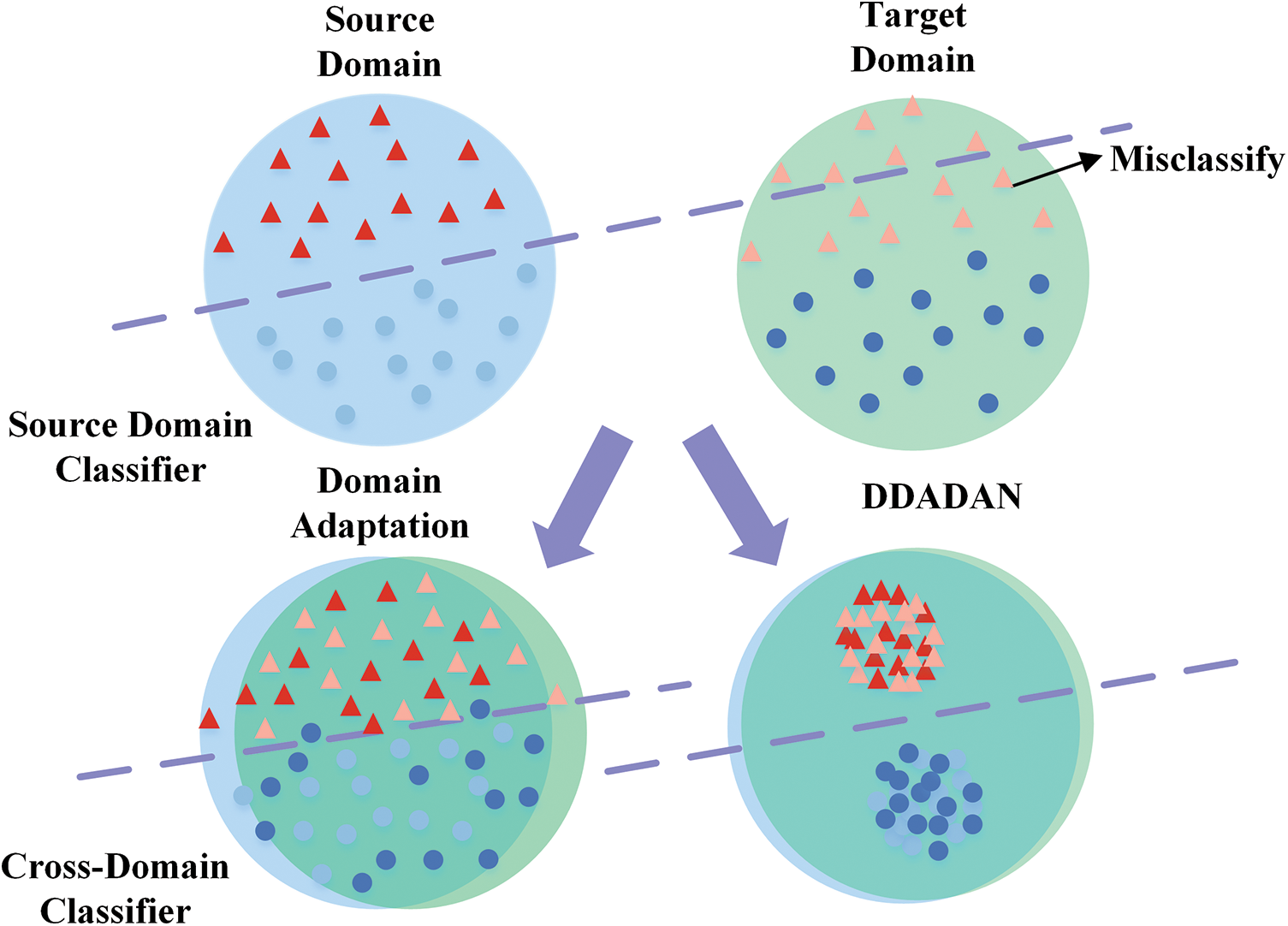
Figure 1: Illustration of the capability of DDADAN. The source domain classifier cannot be directly employed due to the distribution discrepancy. The proposed DDADAN can well bridges the distributional discrepancy and promotes the discriminability of the target domain features

(1) A novel deep adversarial domain adaptation intelligent fault diagnosis method is proposed, which employs IWDCNN as a feature extractor to avoid noise disturbance in the data acquired in industrial environments.

(2) In order to bridge the discrepancy in data distribution between the two domains, a deep correlation alignment is implemented as a discrepancy metric across two domains. Discriminative feature terms are also embedded into the model, which enable features to be clustered within classes and differentiated between classes.

(3) Extensive testing on two sets of bearing fault datasets has revealed that DDADAN outperforms other methods in terms of fault recognition accuracy and generalization capabilities. Experimental analysis and feature visualization show that DDADAN can reduce cross-domain distribution discrepancy, and enhance feature distinguishability.

The following sections of the paper are organized as: An illustration of the domain adaptation problem, accompanied by a brief explanation of the a priori knowledge, is provided in Section 2. Section 3 provides an elaboration on the proposed method. The experiments are presented in Section 4 and the proposed method is evaluated by analyzing the results. Section 5 draws conclusions.

2  Preliminary

2.1 Problem Definition

In this paper, we defined the source domain data as 𝒟s={(xis,yis)}i=1ns, where labels containing machine degradation or fault status information are available. Target domain is defined as 𝒟t={(xjt)}j=1nt. It is the test data, and labels are not usable. Further, the 𝒟s and 𝒟t have the same label space y={0,1,2,…,K−1}. The labels indicate the health status or fault status, respectively. However, since the machine will experience different environment and operation conditions during its service life, 𝒟s and 𝒟t are expected to obey distributions P(X) and Q(X), respectively [36].

In the domain shift problem, sensor data is collected under various operating conditions. A model trained using labeled source domain data has limited adaptability when transferring to unlabeled target domain data. Therefore, the purpose of this paper is to construct a deep discriminative adversarial diagnosis method, which is based on domain adaptation theory. In the constructed method, the extracted features make the domain discriminator difficult to distinguish coming from either the source or the target domain. The domain discriminator then endeavors to differentiate which domain the features come from. Through the performance of such adversarial training, the model learns generalized knowledge.

2.2 Deep Correlation Alignment

The underlying domain-adversarial training can pull the distributions of the two domains closer, but its robustness is limited. Accordingly, the deep correlation alignment algorithm [29] was introduced to improve the model, i.e., a new loss is introduced-the deep CORAL loss (DCORAL). DCORAL is similar to the distance algorithm MMD but its computational cost is cheaper. In contrast to the CORAL algorithm [37], DCORAL overcomes its reliance on linear transformations. It non-linearly aligns second-order statistics from various distributions to extract domain-invariant features. In addition, it is easy to interface DCORAL with deep models [38].

Assuming that CS and CT are the covariance matrices of the source and target domain features, respectively. The DCORAL can be represented as:

Lc=14d2‖CS−CT‖F2(1)

where ‖⋅‖F2 is denoted as the F-norm of the square matrix.

The covariance of the features can be computed as:

CS=1ns−1(Ds⊤Ds−1ns(1⊤Ds)⊤(1⊤Ds))(2)

CT=1nt−1(Dt⊤Dt−1ns(1⊤Dt)⊤(1⊤Dt))(3)

where 1 is a column vector with 1 as each of its elements.

3  Proposed Method

We elaborate on the DDADAN, including the architecture and training procedure in this section.

3.1 DDADAN

To address the discrepancy in fault data distribution under varying operating conditions in the same equipment, we propose a deep discriminative adversarial domain adaptation model. The structure of DDADAN comprises three main components: a feature extractor, a deep discriminative label classifier and a domain discriminator. This is illustrated in Fig. 2. Firstly, the proposed method utilizes IWDCNN to extract deep features from frequency domain signals; Second, the domain discriminator and the deep discriminative label classifier are set up in parallel. The classification labels of samples are predicted using the deep discriminative label classifier; Finally, the domain discriminator is inspired by the adversarial idea and is used to differentiate samples. The domain discriminator is used during training to measure the distribution distance. Simultaneously, DCORAL is performed at the last layer of the feature extractor to bridge distribution discrepancy. The discriminative feature learning is executed at the fully connected layer of the label classifier.

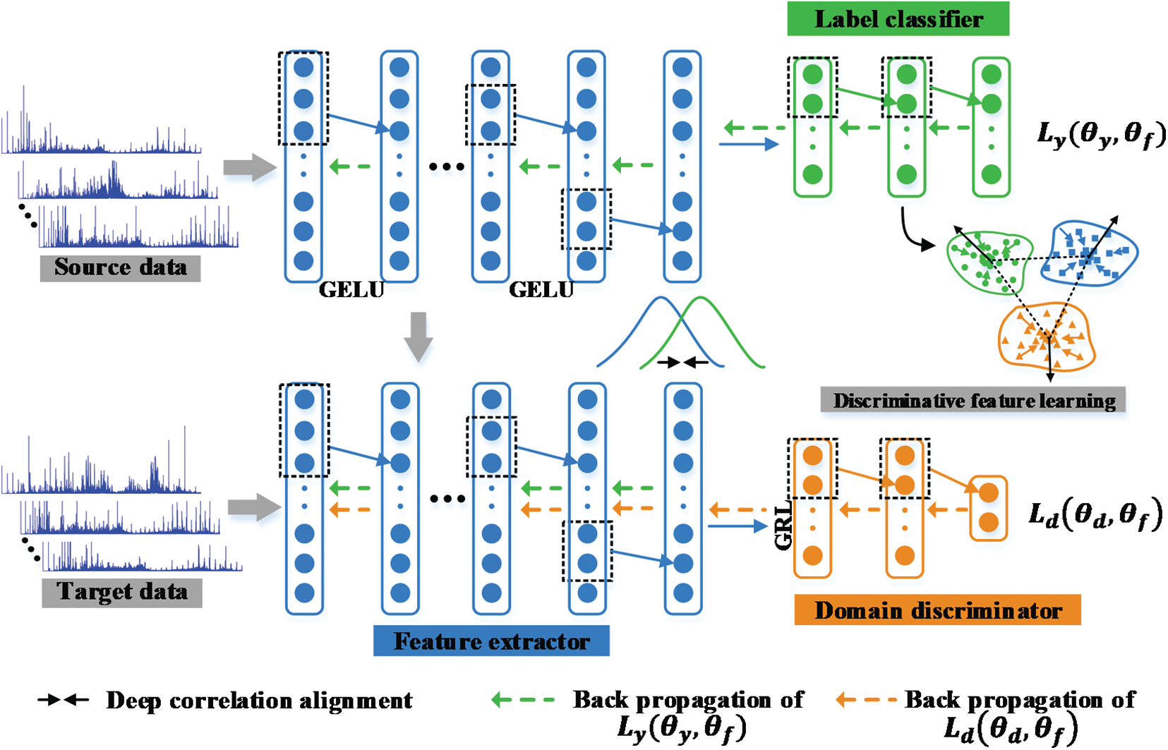
Figure 2: Architecture of the DDADAN model

3.1.1 IWDCNN

As mentioned above, CNNs have been used extensively for fault diagnosis, where some models have not achieved superior performance compared to traditional methods. For one-dimensional signals, the first layer of convolution of the small kernel is prone to cause the model to be disturbed by the high-frequency noise. Meanwhile, large-scale convolutional kernel tends to extract low frequency information and small-scale convolutional kernel inclines to extract high frequency information. Therefore, in order to capture more valuable information in the vibration signal, IWDCNN is proposed as a feature extractor based on WDCNN [26].

Firstly, we employ first convolution layer with a wide kernel to extract features. Four layers of small-scale convolution kernels to deepen the network and obtain high level feature representations. For the j-th convolution kernel, the mathematical expression of the convolution operation is as follows:

cjl(i)=wjl−1∗xl−1(i)+bjl−1(4)

where w and b denote weights and bias; ∗ denotes the convolution operation; and cjl(i) is the output.

After the convolution procedure, the network requires the addition of an activation layer. The activation function enables the network to gather a nonlinear representation of the input signal, which in turn enhances its feature differentiability. The Gaussian Error Linear Unit (GELU) [39] was introduced for improving the model’s generalizability. GELU adds the idea of stochastic regularity to the activation, which is intuitively more in line with natural cognition. The approximate computation of GELU is expressed as:

ajl(i)=GELU(cjl(i))=0.5cjl(i)(1+tanh[2/π(cjl(i)+0.044715(cjl(i))3)])(5)

The parameters of the features are reduced using the max-pooling process to generate shift-invariant features. The mathematical expression of max-pooling is as follows:

pjl(i)=max(i−1)w+1≤u≤iw{ajl(i)}(6)

where pjl(i) denotes the output; (i−1)w+1≤u≤iw denotes the pooling region.

Further, in order to minimize the internal covariance shift and hasten model training, a BN layer is also added. After the convolutional layer and before the activation function, the BN layer is inserted, and the h-dimensional input x=(x1,x2,…,xh) for the BN layer is converted to:

x^i=xi−E[xi]Var[xi](7)

bi=γix^i+βi(8)

where bi is the output, γi corresponds to the scale parameter and βi represents the displacement parameter.

Finally, the last convolutional layer is subjected to global average pooling to accelerate the training process. This allows a significant decrease in network parameters and a direct dimensionality reduction. Global average pooling is defined as:

gjl(i)=average(i−1)w+1≤v≤iw{ajl(i)}(9)

where gjl(i) denotes the output of the average pooling layer; (i−1)w+1≤v≤iw denotes the pooling induction region. A fully connected layer flattens the features on the output into a one-dimensional vector which is then input to the domain discriminator and label classifier.

The combination of the above operations constitutes a feature extractor, which obtains the transferable features. Here we use Gf to represent the feature extractor, where the mapping parameter is θf. Following feature extraction, the source domain input sample xis is transformed into fis=Gf(xis,θf) and the target domain input sample xjt is transformed into fjt=Gf(xjt,θf).

3.1.2 Deep Discriminative Label Classifier

Faults on the source and target domain samples are categorized using the label classifier. The activation function ReLU and the classification function Softmax make up its two fully connected layers. Given a dataset containing K defect classes, the label classifier’s output can be written as:

[p0(x)p1(x)⋯pK−1(x)]=1∑K−1k=0eσkx[eσ0xeσ1x⋯eσKx](10)

where σ denotes the parameters to be learned.

The objective of training the label classifier is to identify the fault types as accurately as possible based on the various classification features. Therefore, it is desired to minimize the loss of labeled classifier during training. We denote the labeled classifier with parameter θy by Gy and its loss Lcl can be calculated by cross-entropy loss as follows:

Lcl(θy,θf)=−∑K−1k=0I[y=k]log⁡pK−1(x)(11)

where I[⋅] is the indicator function.

Discriminative feature learning [40] is introduced as a means to further differentiate the deep features taking into account the intricate relationships between fault classes. Discriminative feature learning, in contrast to center-based loss [41], penalizes the distance between a deep feature and its related class center as well as widens the gap between various class centers. Meanwhile, the computational complexity of center-based discriminative loss is lower, which can be described as follows:

Lce=ε∑nsi=1max(0,‖fis−cyi‖22−m1)+∑K−1i,j=0,i≠jmax(0,m2−‖ci−cj‖22)(12)

where ε is the trade-off parameter and m1 and m2 are two constraint margins; fis denotes the deep feature output of the i-th training sample after feature extraction; cyi denotes the global class center of the yi-th deep feature, yi∈{0,1,2,…,K−1}; ci and cj indicate the batch class centers, which are approximated by averaging the deep features of the current batch. The loss consists of two terms. The former term is intended to measure the intra-class compactness of the features. Its distance between samples within a class is constrained to be no greater than m1. The latter term, which is used to gauge inter-class separability, constrains the distance between intra-class samples to be no less than m2.

To render features more identifiable, the proposed method embeds a center-based discriminative loss term. Therefore, the loss of the final deep discriminative label classifier is given as:

Ly(θy,θf)=Lcl(θy,θf)+φ⋅Lce(13)

where φ is the trade-off parameter.

3.1.3 Domain Discriminator

To obtain domain-invariant features, we introduce the domain discriminator Gd which reduces the data distribution across the two domains. The inspiration for Gd comes from generative adversarial networks (GAN) [42]. There are two fully connected layers in the domain discriminator. LeakyReLU is the first layer’s activation function, and softmax is the second layer. The binary cross-entropy loss function’s estimated loss can be characterized as follows:

Ld(θd,θf)=1n∑ni=1(rilogd(xi)+(1−ri)log(1−d(xi)))(14)

where, d(xi) represents the predicted domain label for the i-th input sample; ri denotes the actual domain label.

For the output of the feature extractor, the above equation can be expressed as:

Ld(θd,θf)=1ns∑nsi=1Ld(θd,θf)(Gf(xis,θf))+1nt∑ntj=1Ld(θd,θf)(Gf(xjt,θf))(15)

where Gf(xis,θf) and Gf(xjt,θf) represent the outputs after the feature extractor.

3.2 Optimization Strategy

The proposed method’s optimization objective necessitates that Gf extract features that may as effectively separate the source and target domains as possible. Meanwhile, Gd is unable to distinguish the difference between the two domains. The total loss can be established as:

L(θf,θy,θd)=Ly(θy,θf)−λ1Ld(θd,θf)+λ2Lc(16)

where λ2 is the trade-off parameter. According to the optimization objective of the proposed method, a set of saddle point parameters θ^f, θ^y, θ^d of the function (16) is sought. Therefore, the following equation holds:

(θ^f,θ^y)=argminθf,θyL(θf,θy,θ^d)(17)

θ^d=argmaxθdL(θ^f,θ^y,θd)(18)

At the saddle point, the parameter θy minimizes the loss of label classification, and θd minimizes the loss of domain discrimination. The parameter θf of the feature extractor minimizes the loss of label classification while maximizing the loss of domain discrimination, i.e., the features are discriminative and having domain invariance. The parameters θf, θy, and θd are updated by back-propagation as follow:

θf←θf−η∂(Ly−λ1Ld+λ2Lc)∂θf(19)

θy←θy−η∂Ly∂θy(20)

θd←θd−η∂Ld∂θd(21)

where η is the learning rate. Due to the −λ1 factor, the parameter update process cannot be directly implemented by stochastic gradient descent. Therefore, a gradient reversal layer (GRL) is introduced among the domain discriminator and the feature extractor. During forward propagation, GRL is only used as a constant transform. In backward propagation, the gradient is obtained from the domain classifier by multiplying it by −λ1, i.e., by −λ1∂Ld∂θf instead of ∂Ld∂θf.

In each iteration, the global class center cyi is modified as follows:

Δcj=∑nbi=1δ(yi=j)(cj−fis)1+∑nbi=1δ(yi=j)(22)

cjt+1=cjt−αΔcjt(23)

where α is the learning rate of the updated global class center; nb is batch size. In the first iteration, the global class center is initialized to the batch class center. The global class center will be in closer proximity to cyi as the number of iterations rises.

3.3 Fault Diagnosis Process of DDADAN

The completed diagnostic procedure for the DDADAN is illustrated in Fig. 3. Firstly, the vibration data is collected by accelerometers, and FFT is employed to gather the required data set. Then, the feature extractor receives input from both the source domain data and the target domain data in order to extract the deep features. The deep discriminative label classifier performs fault classification based on the extracted features. And the domain discriminator predicts the domain labels. The loss function and the total optimization objective are calculated by Eq. (16). Next, the backpropagation algorithm is applied to update the parameters θf, θy, θd. Finally, classification predictions are generated by feeding the test data to the trained model.

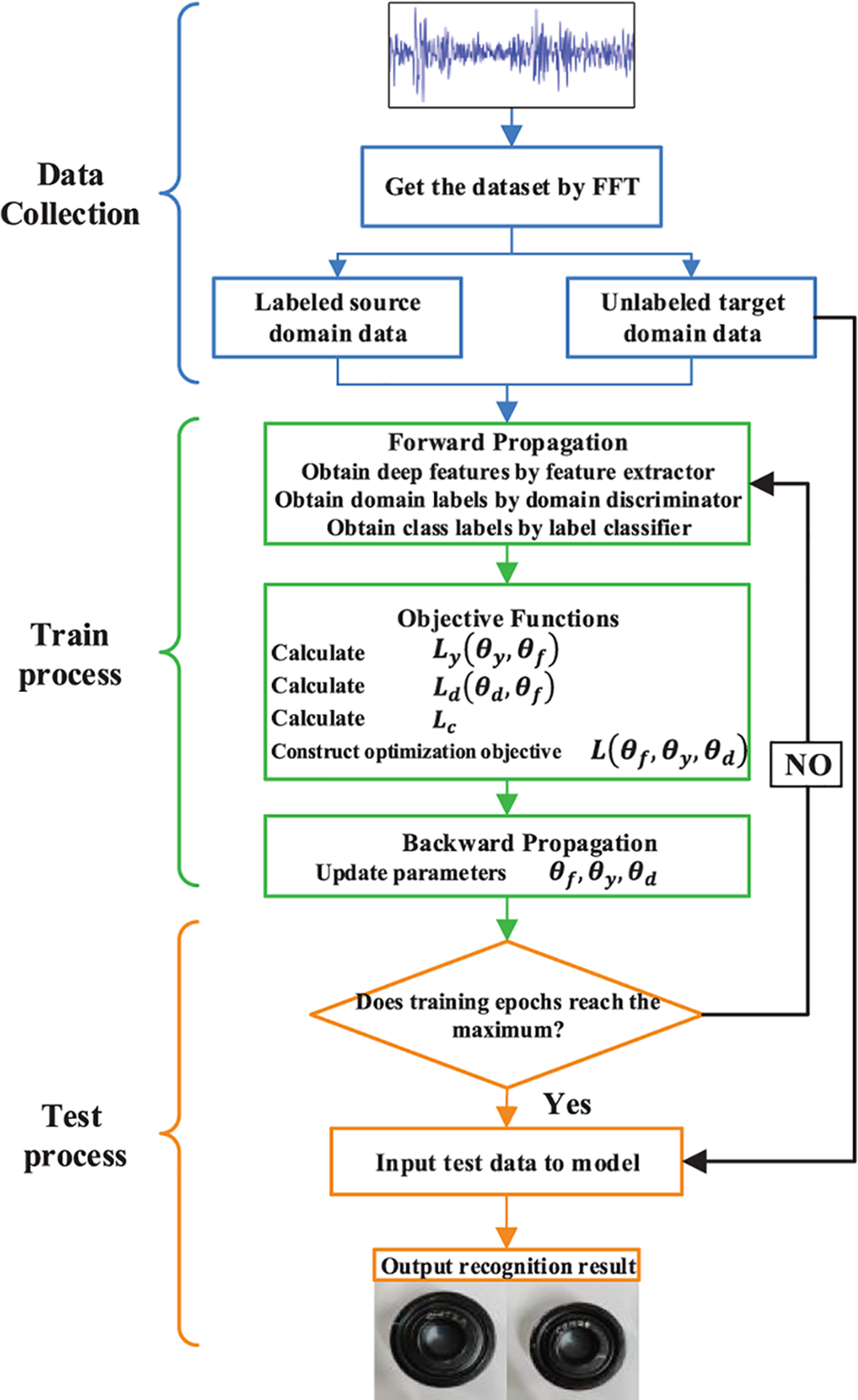
Figure 3: DDADAN fault diagnosis flow chart

4  Experimental Study

In this research, fault diagnostic tests are performed using a set of public bearing datasets and a collection of laboratory datasets to confirm the efficacy of the DDADAN.

4.1 Description of Dataset

4.1.1 Case1: Machinery Fault Simulator (MFS) Dataset

As shown in Fig. 4, the machinery fault simulator test bench mainly includes signal collector, motor control system, tachometer, drive motor, test bearing housing and acceleration sensor. The bearing type of the MFS test bench is MB ER-10K, which parameters are shown in Table 1. The vibration signals of five various health states including ball fault (BF), combined inner ring fault (IRF), normal condition (NC), outer ring fault (ORF) and inner and outer ring fault (CF). The sampling frequency is set to 25.6 KHz. We construct six domain adaptation fault identification tasks: D01, D02, D10, D12, D20 and D21 between three different speeds of 2400, 2800 and 3200 r/min, respectively. D01 indicates that under the same load, the source domain data was acquired at a speed of 2400 r/min and the target domain data was sampled at a speed of 2800 r/min. The source and target domains have sample counts of 100 and 80, respectively, with a sample length of 2048. The frequency domain waveforms of the bearings in five health states at varying rotational speeds are shown in Figs. 5a–5c.

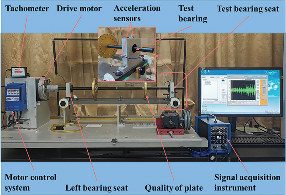
Figure 4: MFS bearing dataset test bench

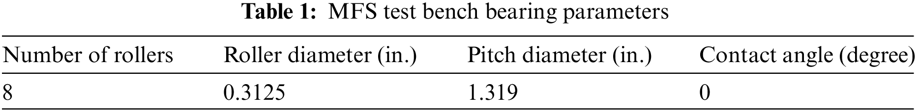
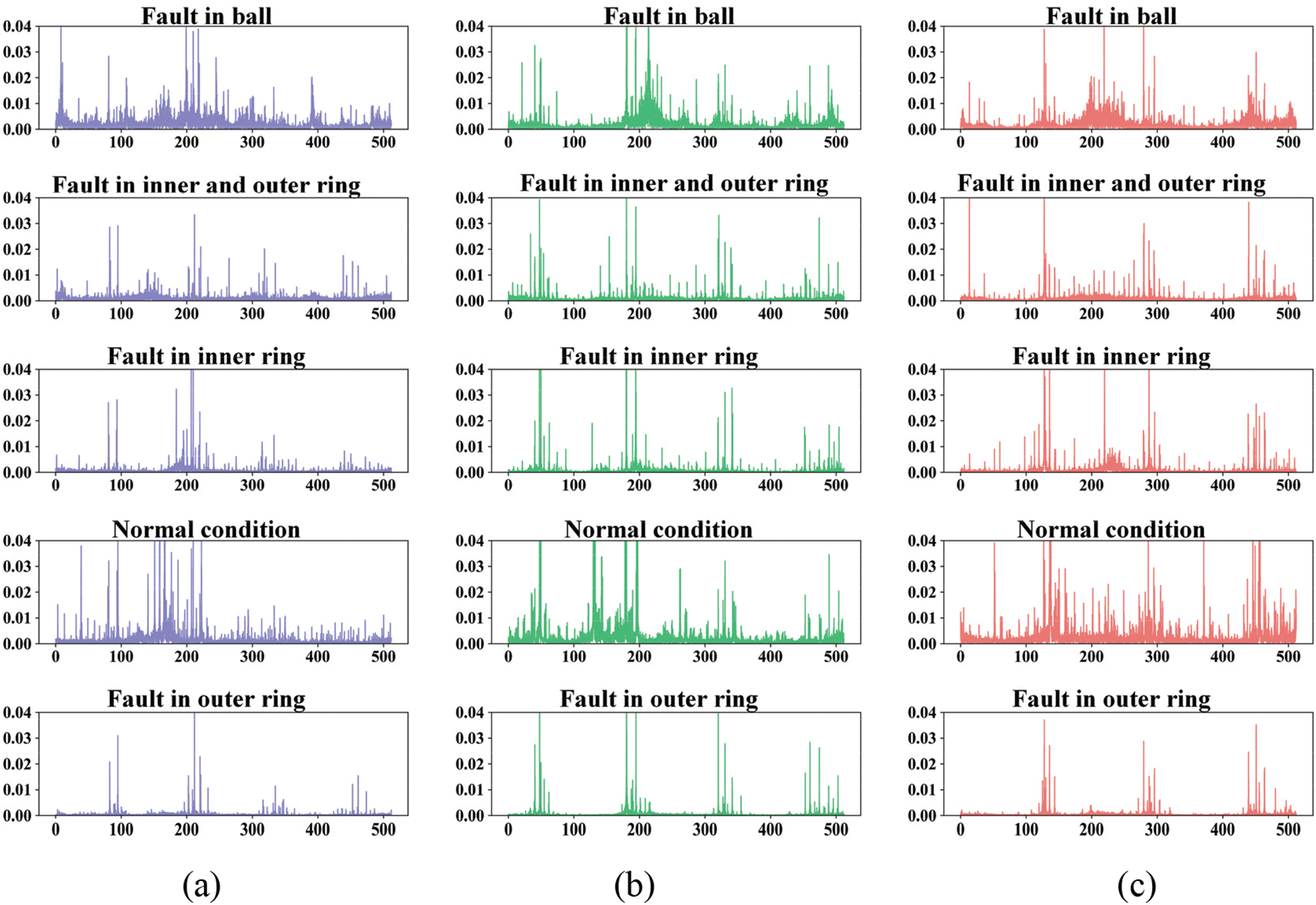
Figure 5: The frequency domain waveforms of the bearings in five health states at varying rotational speeds. (a) 2400 r/min (b) 2800 r/min (c) 3200 r/min

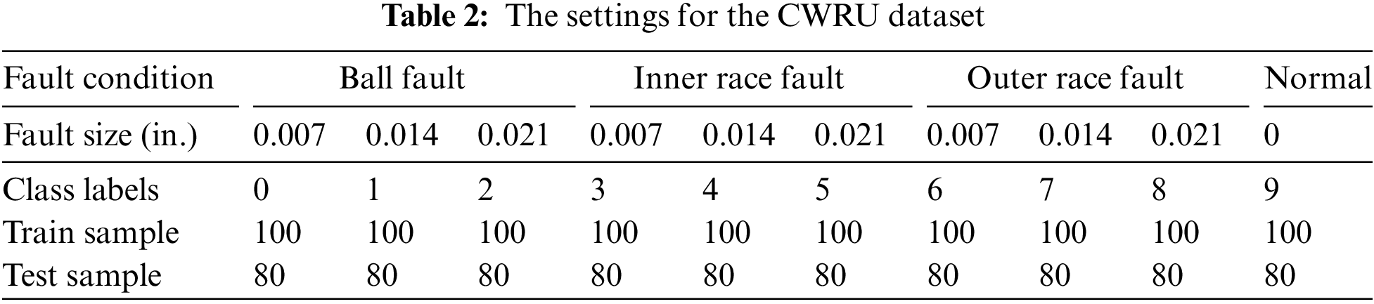
4.1.2 Case2: Case Western Reserve University (CWRU) Dataset

The CWRU dataset [43] is used as experimental data for fault classification, and its experimental setup is shown in Fig. 6. The testing bench mainly includes sensors, an electric motor and dynamometer, etc. We chose a 12 kHz drive end vibration acceleration signal with dynamometer-generated rated loads of 0, 1, 2, and 3 hp. Bearing fault data include, in addition to normal condition, ball fault, inner ring fault and outer ring fault. Each fault state introduces three damage diameters: 0.007, 0.014 and 0.021 inch, separately. Therefore, there are ten different fault conditions under each load. To examine the performance of the proposed DDADAN, 12 transfer tasks are constructed across varied loads. The transfer tasks are designated as C01, C02, C03, C10, C12, C13, C20, C21, C23, C30, C31, C32, respectively. Table 2 gives the settings for the CWRU dataset.

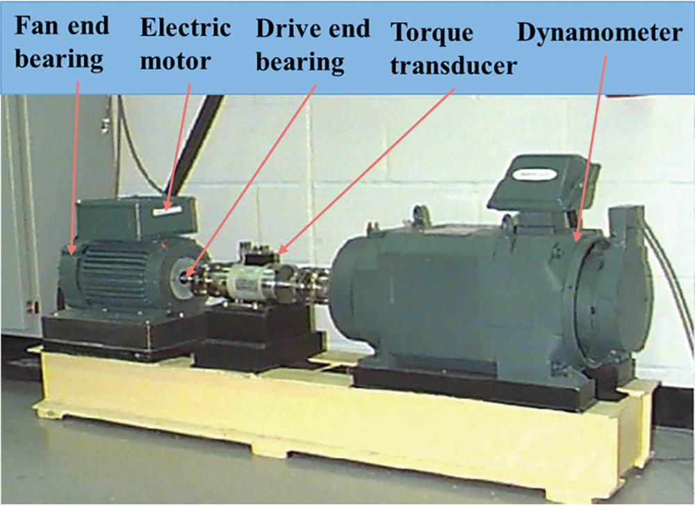
Figure 6: CWRU bearing dataset test bench

4.2 Methods Comparison

CNN: Convolutional neural network (CNN) [44] is a typical deep model used extensively in fault diagnosis. CNN is trained with source domain data as one of the comparative methods.

DANN: DANN [45] is one of the most representative models of DA. DANN has been configured to have the same structure and parameters as DDADAN.

MMD: MMD [46] is a broadly used discrepancy metric that facilitates network acquisition of transferable features. The MMD-based method shares the same network parameters with DDADAN, which is added MMD loss to its optimization objective.

EntMin: Entropy minimization (EntMin) [47] is performed by reducing the Shannon entropy of the batch output matrix in the target domain, which reduces the prediction uncertainty. There is significance in combining the base model with EntMin as one of the comparison methods.

To ensure a fair comparison, identical hyperparameters were adopted for all methods to be updated by the Adam optimizer. The batch size was chosen to be 64 and the learning rate η was adjusted to 0.002. The trade-off parameter λ1 is progressively raised from 0 to 1 for all DA methods using the following formula:

λ1=21+exp⁡(−10g)−1(24)

where g is the global training step of DDADAN. The parameter λ2 is set to 0.02 and φ is set to 0.2. For discriminative feature learning, the parameter ε is fixed to 0.5 and the learning rate of class center α is set to 0.05. The constraint margins m1 and m2 are set to 0 and 100, respectively.

4.3 Experimental Results of the Dataset

4.3.1 Case1: Experimental Results of the MFS Dataset

Ten experiments were conducted for all four methods under the established six domain adaption fault identification task. Also, to eliminate coincidences, there were ten repetitions of the experiment for each transfer task. The accuracy obtained is the average of the results of ten trials. The final obtained fault classification accuracy of DDADAN and the comparison methods are shown in Table 3. It is noticeable that the highest classification accuracy of CNN is only 81.92%. That indicates without transfer learning, diagnosis methods would perform poorly in cross-domain tasks. DANN method learns domain invariant features and achieves an average accuracy of 92.35%. However, it will suffer from a lack of transfer capability when faced with certain tasks. The MMD method aligns the marginal distributions of the source and target domains, and the diagnostic accuracy is improved up to 97.67%. The EntMin method reduces the uncertainty of target domain prediction, achieving an average accuracy of 96.59%. Compared with the MMD method, the proposed method enhances the discrimination of the target domain in addition to the aligned data distribution. Higher accuracy is achieved on different transfer tasks, with an average accuracy of 98.89%. For tasks D02 and D20 with large discrepancy of data, the diagnostic accuracy of the DDADAN can still achieve more than 97.53%. Fig. 7 gives a comparison of the accuracy of several methods of fault diagnosis.

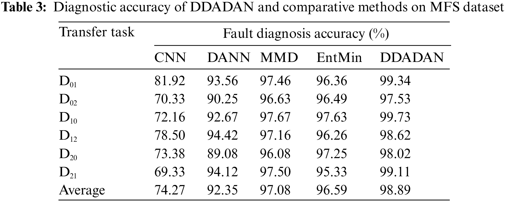
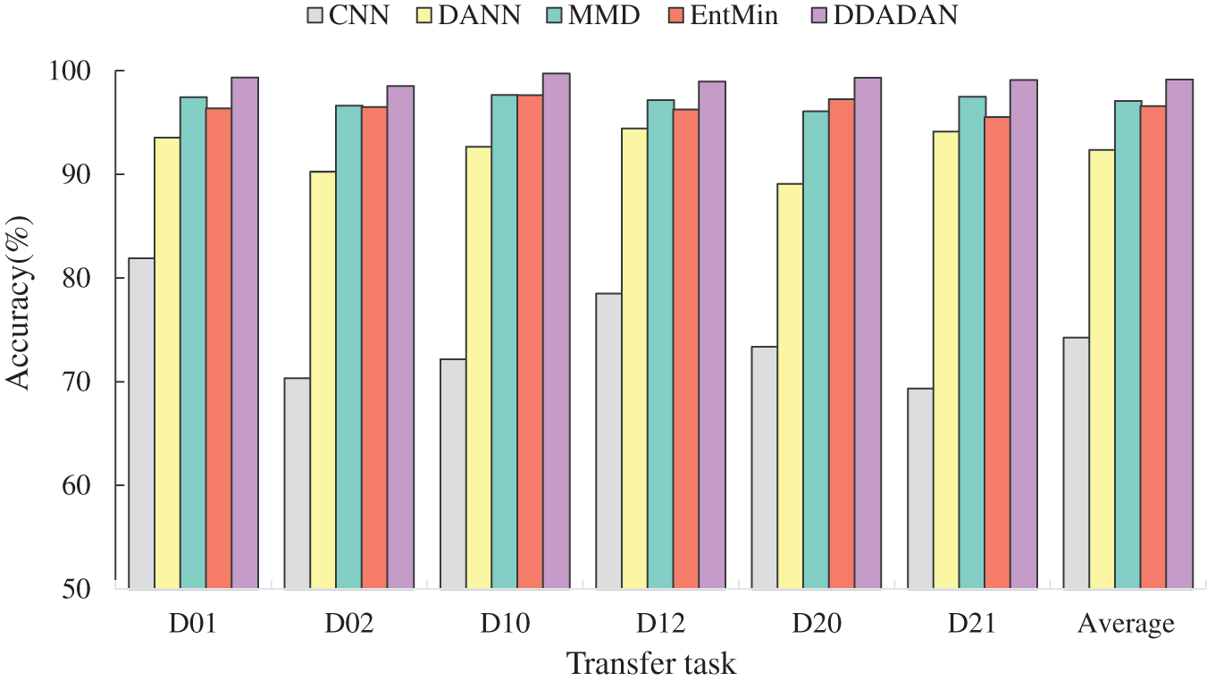
Figure 7: Comparison of the performance of several methods on the MFS dataset

In order to obtain a more comprehensive understanding of the distribution of the learned features, we apply the t-Distributed Stochastic Neighbor Embedding (t-SNE) [48]. The transfer tasks from 2400 to 2800 r/min were picked and reduced the data to two dimensions for visualization. The features of the proposed method and the comparison method at the fully connected layer are shown in Fig. 8. Evidently, the CNN without transfer learning extracts data with a significant discrepancy in distribution, which is difficult to provide accurate identification of target domain samples. Fig. 8d shows that DANN learns more domain invariant features, which is still having large discrepancy in the data distribution. The MMD-based method obtains better results by bridging the data distribution through the discrepancy metric, as shown in Fig. 8c. However, MMD’s classification boundary is hazy, which shows lacking discriminative capacity. Since EntMin reduces the prediction uncertainty, which makes the target domain samples have improved discriminability. As shown in Fig. 8b, the EntMin method misclassifies the fault samples class CRF to the BF, which shows it will result in losing the original class diversity of the samples. As seen in Fig. 8a, features from various classes are simpler to distinguished and features from the same class turn more compact. This implies that the model is able to employ discriminative feature learning to acquire more distinct features.

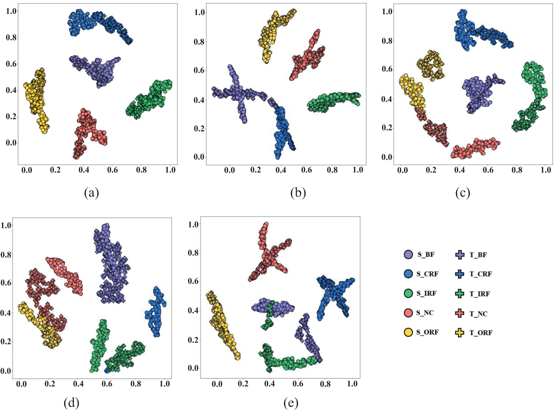
Figure 8: Varying methods for t-SNE visualization on the MFS dataset. (a) DDADAN (b) EntMin (c) MMD (d) DANN (e) CNN

4.3.2 Case2: Experimental Results of the CWRU Dataset

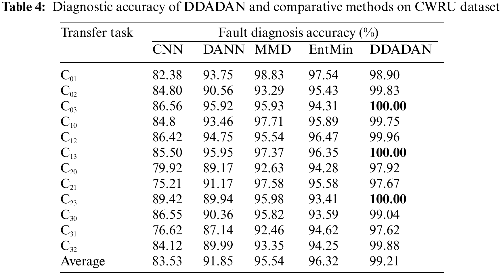
The diagnostic accuracy of DDADAN and comparative methods on CWRU dataset is shown in Table 4. For different transfer tasks, it can be observed that the proposed DDADAN achieves a high accuracy. The accuracy of the CNN method is only 83.53% on average. DANN achieves an average diagnostic accuracy of 92.35% through adversarial training. In the face of some transfer tasks, it still has inadequate diagnostic capability. The MMD-based method aligns the distributions of the both domains. However, the target domain samples are not discriminatory enough. The EntMin-based method achieves an average accuracy of 96.32%, except that its reduction of target domain prediction uncertainty may contribute to lower prediction diversity. The accuracy of the proposed DDADAN is more than 2.89% higher than other methods. Correlation alignment is introduced to guide domain adversarial training, and the discriminative loss terms in the aligned feature space make the target domain samples more distinguishable.

For clear overview of the features learned by several methods, the features are visualized utilizing t-SNE. As shown in Fig. 9a, the proposed DDADAN well bridges the data distribution discrepancy, and has distinct classification boundaries. The remaining four methods are not sufficient in bridging the distribution.

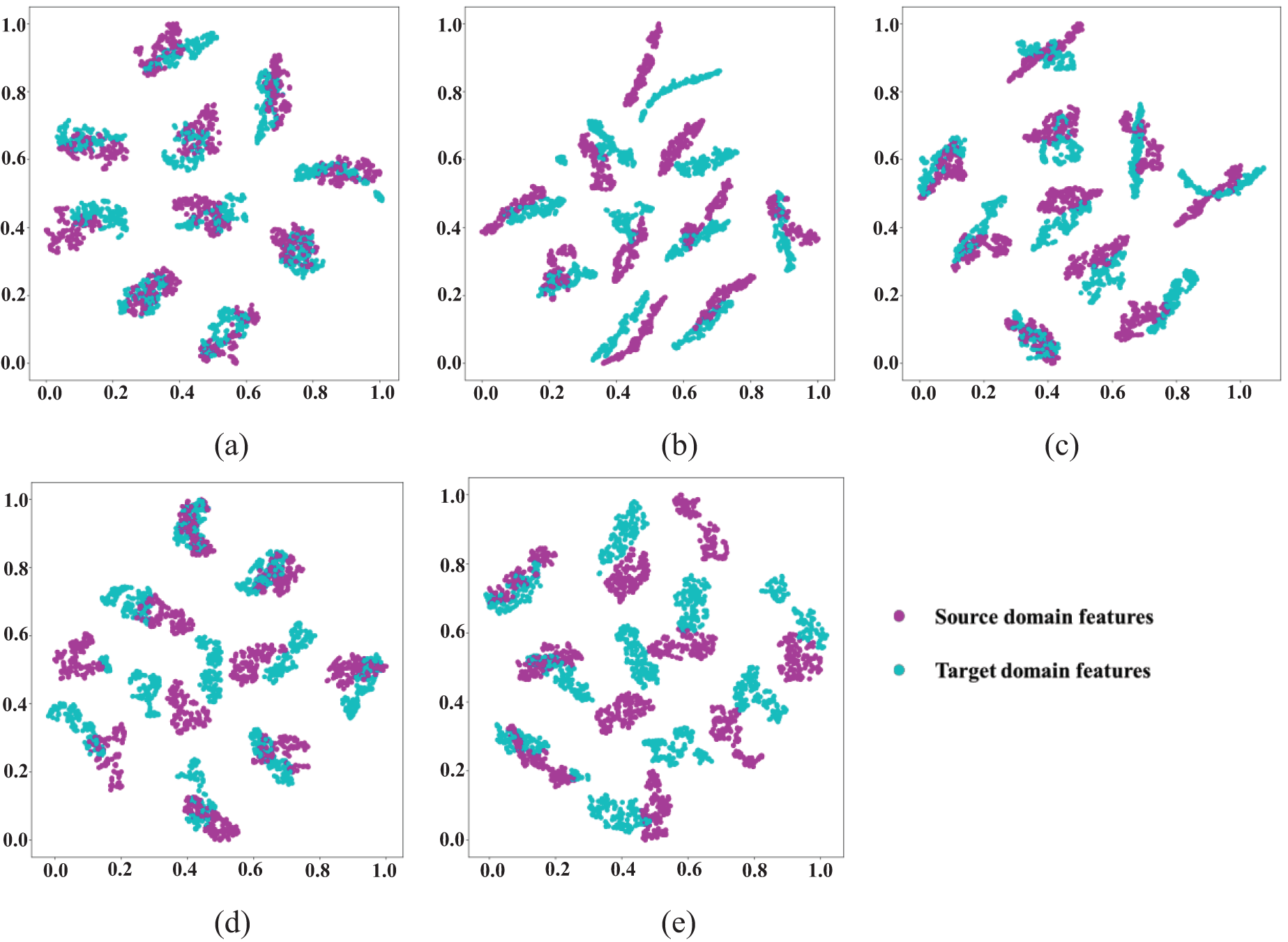
Figure 9: Varying methods for t-SNE visualization on the CWRU dataset. (a) DDADAN (b) EntMin (c) MMD (d) DANN (e) CNN

Fig. 10 displays the confusion matrix of the DDADAN and compared methods for the transfer task C03. The CNN-based method performs poorly against the cross-domain task, with multiple misdiagnosis and missed diagnosis cases. In contrast, there is a large improvement in fault recognition of DANN, and the misclassification cases are basically only present on ball faults with different fault sizes. Fewer outer ring fault features with sizes of 0.021 in. have been mistaken for other fault types using the MMD-based fault diagnosis method. Notably, the EntMin method failed to detect the ball fault with 0.021 in. This suggests that although the EntMin method enhances the discriminability of the target domain, there might be a loss of its predictive class diversity. With the suppression of high-frequency noise in the input data and the enhancement of the discriminability of the features, the proposed method can accomplish the accurate identification of various faults.

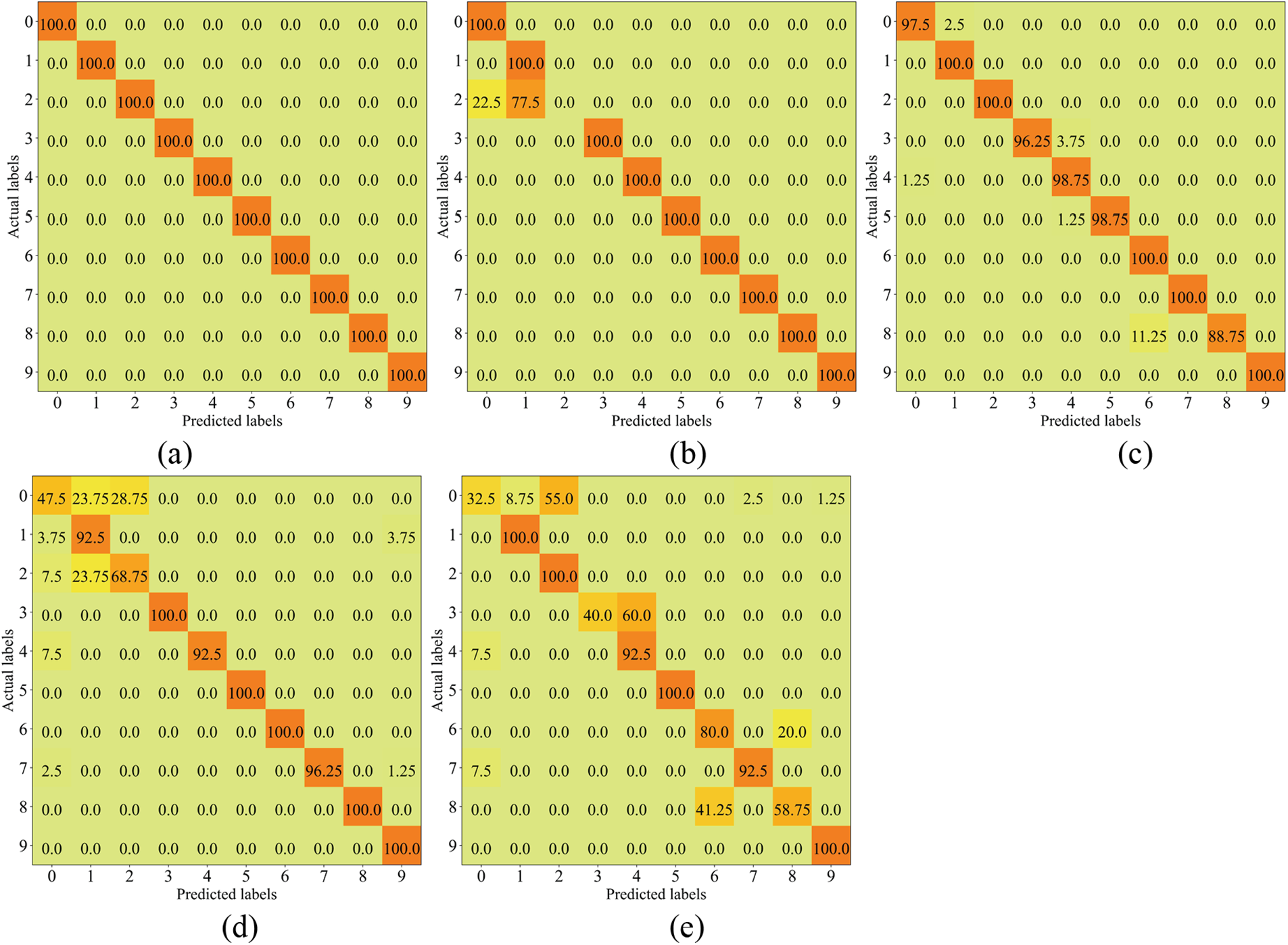
Figure 10: Test samples confusion matrix of the varying method on the transfer task C03 (a) DDADAN (b) EntMin (c) MMD (d) DANN (e) CNN

4.4 Experiment in Noisy Environment

Environmental noise is unavoidable in industrial settings, therefore being a challenge for extracting signal features. We opted to introduce Gaussian white noise to the vibration signal in order to test the suggested method’s noise immunity. To replicate the industrial environment, which may be exposed to a range of noise levels, noise with varied signal-to-noise ratios (SNR) is added:

SNRdB=10log10⁡(PsignalPnoise)(25)

In our experiments, different models are trained by the dataset from MFS. The results of the migration task D12 are shown in Fig. 11. From the figure, it can be seen that the diagnostic accuracy of different models is affected to different degrees under the noisy environment, and the accuracy shows a decreasing trend with the decrease of SNR. The proposed method’s diagnostic accuracy is more negatively impacted when the SNR=−6dB, and the accuracy is only about 92% properly. CNN and DANN have less than 70% diagnostic accuracy under the noise with SNR=−6dB. Since the MMD method has the same feature extractor as the DDADAN, diagnosis accuracy can be maintained under different noise environments. DDADAN can maintain more than 97% accuracy under noise with SNR≥0dB. Using the IWDCNN as a feature extractor implies that high frequency noise can be effectively suppressed. In noisy environments, the suggested method can maintain high diagnostic accuracy.

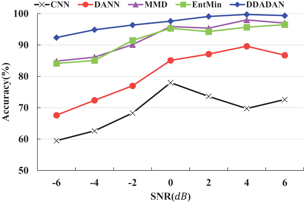
Figure 11: Diagnostic accuracy of models under different noise

5  Conclusion

A deep discriminative adversarial domain adaptation method is proposed for fault identification to address the distribution discrepancy of fault data in bearings under various operating conditions. Firstly, the IWDCNN is employed to extract the deep features of the fault data. Then, domain-invariant features are learned from fault data using correlation alignment-based domain adversarial training, which measures the distribution between two domains. Finally, discriminative feature learning is incorporated into this network to make the features intra-class compact and inter-class separable. To confirm the performance of the proposed method, a public dataset and a laboratory dataset are analyzed. The experimental results demonstrate that DDADAN can perform a variety of transfer tasks with high accuracy and robustness. The proposed method can still achieve an accuracy of more than 97.53% when dealing with the transfer diagnosis task with significant speed discrepancy. At the same time, experiments are conducted under various noise levels, and the findings prove that the DDADAN has effective noise-cancelling capabilities.

Since there is a labeling offset in the data gathered under varying working conditions, the proposed method has limitations for fault identification in practical industrial circumstances. Therefore, we will continue to research ways to improve fault diagnostic capabilities when the label spaces of the two domains differ. Additionally, one of the future studies is the development of knowledge graph for fault diagnosis under non-stationary conditions.

Acknowledgement: We extend our gratitude to the peer reviewers for their helpful comments on an earlier version of the paper.

Funding Statement: This work was supported by the Natural Science Foundation of Henan Province (232300420094) and the Science and Technology Research Project of Henan Province (222102220092).

Author Contributions: The authors confirm contribution to the paper as follows: study conception and design: Jie Wu; manuscript writing and software: Jinxi Guo; Kai Chen; data collection and validation: Yuhao Ma; analysis and interpretation of results: Jianshen Li. Xiaofeng Xue; manuscript review and supervision: Jiehui Liu; manuscript translation and editing: Yaochun Wu. All authors reviewed the results and approved the final version of the manuscript.

Availability of Data and Materials: The data used to support the findings of this study are available from the corresponding author upon request.

Conflicts of Interest: The authors declare that they have no conflicts of interest to report regarding the present study.

References

1. Yang, B., Lei, Y., Jia, F., Xing, S. (2019). An intelligent fault diagnosis approach based on transfer learning from laboratory bearings to locomotive bearings. Mechanical Systems and Signal Processing, 122, 692–706. https://doi.org/10.1016/j.ymssp.2018.12.051 [Google Scholar] [CrossRef]

2. Zhou, Z., Ming, Z., Wang, J., Tang, S., Cao, Y. et al. (2023). A Novel belief rule-based fault diagnosis method with interpretability. Computer Modeling in Engineering & Sciences, 136(2), 1165–1185. https://doi.org/10.32604/cmes.2023.025399 [Google Scholar] [CrossRef]

3. Liu, R., Yang, B., Zio, E., Chen, X. (2018). Artificial intelligence for fault diagnosis of rotating machinery: A review. Mechanical Systems and Signal Processing, 108(7), 33–47. https://doi.org/10.1016/j.ymssp.2018.02.016 [Google Scholar] [CrossRef]

4. Zhi, P. P., Wang, Z., Chen, B., Sheng, Z. (2022). Time-variant reliability-based multi-objective fuzzy design optimization for anti-roll torsion bar of EMU. Computer Modeling in Engineering & Sciences, 131(2), 1001–1022. https://doi.org/10.32604/CMES.2022.019835 [Google Scholar] [CrossRef]

5. Meng, D., Yang, S., Lin, T., Wang, J., Yang, H. et al. (2022). RBMDO using gaussian mixture model-based second-order mean-value saddle point approximation. Computer Modeling in Engineering and Sciences, 132(2), 553–568. https://doi.org/10.32604/cmes.2022.020756 [Google Scholar] [CrossRef]

6. Xia, M., Li, T., Xu, L., Liu, L., de Silva, C. W. (2017). Fault diagnosis for rotating machinery using multiple sensors and convolutional neural networks. IEEE/ASME Transactions on Mechatronics, 23(1), 101–110. https://doi.org/10.1109/TMECH.2017.2728371 [Google Scholar] [CrossRef]

7. Wu, C., Jiang, P., Ding, C., Feng, F., Chen, T. (2019). Intelligent fault diagnosis of rotating machinery based on one-dimensional convolutional neural network. Computers in Industry, 108(1), 53–61. https://doi.org/10.1016/j.compind.2018.12.001 [Google Scholar] [CrossRef]

8. Jin, X., Feng, J., Du, S., Li, G., Zhao, Y. (2014). Rotor fault classification technique and precision analysis with kernel principal component analysis and multi-support vector machines. Journal of Vibroengineering, 16(5), 2582–2592. [Google Scholar]

9. Lei, Y., He, Z., Zi, Y. (2009). A combination of WKNN to fault diagnosis of rolling element bearings. Journal of Vibration and Acoustics-Transactions of the ASME, 131(6), 1980–1998. https://doi.org/10.1115/1.4000478 [Google Scholar] [CrossRef]

10. Zhong, B., MacIntyre, J., He, Y., Tait, J. (1999). High order neural networks for simultaneous diagnosis of multiple faults in rotating machines. Neural Computing & Applications, 8(3), 189–195. https://doi.org/10.1007/s005210050021 [Google Scholar] [CrossRef]

11. Lu, C., Wang, Z. Y., Qin, W. L., Ma, J. (2017). Fault diagnosis of rotary machinery components using a stacked denoising autoencoder-based health state identification. Signal Processing, 130, 377–388. https://doi.org/10.1016/j.sigpro.2016.07.028 [Google Scholar] [CrossRef]

12. Jiang, H., Shao, H., Chen, X., Huang, J. (2018). A feature fusion deep belief network method for intelligent fault diagnosis of rotating machinery. Journal of Intelligent & Fuzzy Systems, 34(6), 3513–3521. https://doi.org/10.3233/JIFS-169530 [Google Scholar] [CrossRef]

13. Wang, F., Jiang, H. K., Shao, H. D., Duan, W. J., Wu, S. P. (2017). An adaptive deep convolutional neural network for rolling bearing fault diagnosis. Measurement Science and Technology, 28(9), 095005. https://doi.org/10.1088/1361-6501/aa6e22 [Google Scholar] [CrossRef]

14. Zhao, M., Kang, M., Tang, B., Pecht, M. (2017). Deep residual networks with dynamically weighted wavelet coefficients for fault diagnosis of planetary gearboxes. IEEE Transactions on Industrial Electronics, 65(5), 4290–4300. https://doi.org/10.1109/tie.2017.2762639 [Google Scholar] [CrossRef]

15. Meng, D., Yang, S., de Jesus, A. M., Zhu, S. P. (2023). A novel Kriging-model-assisted reliability-based multidisciplinary design optimization strategy and its application in the offshore wind turbine tower. Renewable Energy, 203(12), 407–420. https://doi.org/10.1016/j.renene.2022.12.062 [Google Scholar] [CrossRef]

16. Tian, Z., Zhi, P., Guan, Y., Feng, J., Zhao, Y. (2023). An effective single loop Kriging surrogate method combing sequential stratified sampling for structural time-dependent reliability analysis. In: Structures, vol. 53, pp. 1215–1224. London, England. https://doi.org/10.1016/J.ISTRUC.2023.05.022 [Google Scholar] [CrossRef]

17. Lei, Y., Yang, B., Jiang, X., Jia, F., Li, N. et al. (2020). Applications of machine learning to machine fault diagnosis: A review and roadmap. Mechanical Systems and Signal Processing, 138(2005), 106587. https://doi.org/10.1016/j.ymssp.2019.106587 [Google Scholar] [CrossRef]

18. Li, T., Zhao, Z., Sun, C., Yan, R., Chen, X. (2021). Domain adversarial graph convolutional network for fault diagnosis under variable working conditions. IEEE Transactions on Instrumentation and Measurement, 70, 1–10. https://doi.org/10.1109/TIM.2021.3075016 [Google Scholar] [CrossRef]

19. Li, X., Zhang, W., Ding, Q. (2018). Cross-domain fault diagnosis of rolling element bearings using deep generative neural networks. IEEE Transactions on Industrial Electronics, 66(7), 5525–5534. https://doi.org/10.1109/TIE.2018.2868023 [Google Scholar] [CrossRef]

20. Meng, D., Yang, S., He, C., Wang, H., Lv, Z. et al. (2022). Multidisciplinary design optimization of engineering systems under uncertainty: A review. International Journal of Structural Integrity, 13(4), 565–593. https://doi.org/10.1108/IJSI-05-2022-0076 [Google Scholar] [CrossRef]

21. Ding, Y., Jia, M., Zhuang, J., Cao, Y., Zhao, X. et al. (2023). Deep imbalanced domain adaptation for transfer learning fault diagnosis of bearings under multiple working conditions. Reliability Engineering & System Safety, 230(7), 108890. https://doi.org/10.1016/j.ress.2022.108890 [Google Scholar] [CrossRef]

22. Lu, W., Liang, B., Cheng, Y., Meng, D., Yang, J. et al. (2016). Deep model based domain adaptation for fault diagnosis. IEEE Transactions on Industrial Electronics, 64(3), 2296–2305. https://doi.org/10.1109/TIE.2016.2627020 [Google Scholar] [CrossRef]

23. Zhao, Z., Zhang, Q., Yu, X., Sun, C., Wang, S. et al. (2021). Applications of unsupervised deep transfer learning to intelligent fault diagnosis: A survey and comparative study. IEEE Transactions on Instrumentation and Measurement, 70, 1–28. https://doi.org/10.1109/TIM.2021.3116309 [Google Scholar] [CrossRef]

24. Xu, G., Liu, M., Jiang, Z., Shen, W., Huang, C. (2019). Online fault diagnosis method based on transfer convolutional neural networks. IEEE Transactions on Instrumentation and Measurement, 69(2), 509–520. https://doi.org/10.1109/TIM.2019.2902003 [Google Scholar] [CrossRef]

25. Zhao, B., Zhang, X., Zhan, Z., Pang, S. (2020). Deep multi-scale convolutional transfer learning network: A novel method for intelligent fault diagnosis of rolling bearings under variable working conditions and domains. Neurocomputing, 407, 24–38. https://doi.org/10.1016/j.neucom.2020.04.073 [Google Scholar] [CrossRef]

26. Zhang, W., Peng, G., Li, C., Chen, Y., Zhang, Z. (2017). A new deep learning model for fault diagnosis with good anti-noise and domain adaptation ability on raw vibration signals. Sensors, 17(2), 425. https://doi.org/10.3390/s17020425 [Google Scholar] [PubMed] [CrossRef]

27. Zhang, B., Li, W., Li, X. L., Ng, S. K. (2018). Intelligent fault diagnosis under varying working conditions based on domain adaptive convolutional neural networks. IEEE Access, 6, 66367–66384. https://doi.org/10.1109/ACCESS.2018.2878491 [Google Scholar] [CrossRef]

28. Qian, W., Li, S., Yi, P., Zhang, K. (2019). A novel transfer learning method for robust fault diagnosis of rotating machines under variable working conditions. Measurement, 138, 514–525. https://doi.org/10.1016/j.measurement.2019.02.073 [Google Scholar] [CrossRef]

29. Sun, B., Saenko, K. (2016). Deep coral: Correlation alignment for deep domain adaptation. Computer Vision–ECCV 2016 Workshops, pp. 443–450. Amsterdam, The Netherlands, Springer International Publishing. [Google Scholar]

30. Huo, C., Jiang, Q., Shen, Y., Qian, C., Zhang, Q. (2022). New transfer learning fault diagnosis method of rolling bearing based on ADC-CNN and LATL under variable conditions. Measurement, 188(10), 110587. https://doi.org/10.1016/j.measurement.2021.110587 [Google Scholar] [CrossRef]

31. Wang, Q., Michau, G., Fink, O. (2019). Domain adaptive transfer learning for fault diagnosis. 2019 Prognostics and System Health Management Conference (PHM-Paris), pp. 279–285. Paris, France. IEEE. [Google Scholar]

32. Wang, Y., Sun, X., Li, J., Yang, Y. (2020). Intelligent fault diagnosis with deep adversarial domain adaptation. IEEE Transactions on Instrumentation and Measurement, 70, 1–9. https://doi.org/10.1109/TIM.2021.3123218 [Google Scholar] [CrossRef]

33. Jiao, J., Zhao, M., Lin, J., Liang, K. (2020). Residual joint adaptation adversarial network for intelligent transfer fault diagnosis. Mechanical Systems and Signal Processing, 145, 106962. https://doi.org/10.1016/j.ymssp.2020.106962 [Google Scholar] [CrossRef]

34. Chen, Z., He, G., Li, J., Liao, Y., Gryllias, K. et al. (2020). Domain adversarial transfer network for cross-domain fault diagnosis of rotary machinery. IEEE Transactions on Instrumentation and Measurement, 69(11), 8702–8712. https://doi.org/10.1109/TIM.2020.2995441 [Google Scholar] [CrossRef]

35. Yu, X., Zhao, Z., Zhang, X., Sun, G., Gong, B. et al. (2020). Conditional adversarial domain adaptation with discrimination embedding for locomotive fault diagnosis. IEEE Transactions on Instrumentation andMeasurement, 70, 1–12. https://doi.org/10.1609/AAAI.V33I01.33013296 [Google Scholar] [CrossRef]

36. Han, T., Liu, C., Yang, W., Jiang, D. (2019). A novel adversarial learning framework in deep convolutional neural network for intelligent diagnosis of mechanical faults. Knowledge-Based Systems, 165(6), 474–487. https://doi.org/10.1016/j.knosys.2018.12.019 [Google Scholar] [CrossRef]

37. Sun, B., Feng, J., Saenko, K. (2017). Correlation alignment for unsupervised domain adaptation. Domain Adaptation in Computer Vision Applications, 153–171. https://doi.org/10.48550/arXiv.1612.01939 [Google Scholar] [CrossRef]

38. Qian, Q., Qin, Y., Luo, J., Wang, Y., Wu, F. (2023). Deep discriminative transfer learning network for cross-machine fault diagnosis. Mechanical Systems and Signal Processing, 186(18), 109884. https://doi.org/10.1016/j.ymssp.2022.109884 [Google Scholar] [CrossRef]

39. Hendrycks, D., Gimpel, K. (2016). Gaussian error linear units (GELUs). https://doi.org/10.48550/arXiv.1606.08415 [Google Scholar] [CrossRef]

40. Chen, C., Chen, Z., Jiang, B., Jin, X. (2019). Joint domain alignment and discriminative feature learning for unsupervised deep domain adaptation. Proceedings of the AAAI Conference on Artificial Intelligence, vol. 33, no. 1, pp. 3296–3303. https://doi.org/10.1609/AAAI.V33I01.33013296 [Google Scholar] [CrossRef]

41. Wen, Y., Zhang, K., Li, Z., Qiao, Y. (2016). A discriminative feature learning approach for deep face recognition. Computer Vision–ECCV 2016, pp. 499–515. Amsterdam, The Netherlands, Springer International Publishing. [Google Scholar]

42. Radford, A., Metz, L., Chintala, S. (2015). Unsupervised representation learning with deep convolutional generative adversarial networks. https://doi.org/10.48550/arXiv.1511.06434 [Google Scholar] [CrossRef]

43. Smith, W. A., Randall, R. B. (2015). Rolling element bearing diagnostics using the case Western reserve university data: A benchmark study. Mechanical Systems and Signal Processing, 64, 100–131. https://doi.org/10.1016/j.ymssp.2015.04.021 [Google Scholar] [CrossRef]

44. Krizhevsky, A., Sutskever, I., Hinton, G. E. (2012). ImageNet classification with deep convolutional neural networks. Advances in Neural Information Processing Systems, 25. https://doi.org/10.1145/3065386 [Google Scholar] [CrossRef]

45. Ganin, Y., Lempitsky, V. (2015). Unsupervised domain adaptation by backpropagation. International Conference on Machine Learning, pp. 1180–1189. Lille, France, PMLR. https://doi.org/10.48550/arXiv.1409.7495 [Google Scholar] [CrossRef]

46. Borgwardt, K. M., Gretton, A., Rasch, M. J., Kriegel, H. P., Schölkopf, B. et al. (2006). Integrating structured biological data by kernel maximum mean discrepancy. Bioinformatics, 22(14), e49–e57. New York, USA. https://doi.org/10.1093/bioinformatics/btl242 [Google Scholar] [PubMed] [CrossRef]

47. Grandvalet, Y., Bengio, Y. (2004). Semi-supervised learning by entropy minimization. Advances in Neural Information Processing Systems, 17, 529–536. [Google Scholar]

48. van der Maaten, L. (2014). Accelerating t-SNE using tree-based algorithms. The Journal of Machine Learning Research, 15(1), 3221–3245. [Google Scholar]