Block Incremental Dense Tucker Decomposition with Application to Spatial and Temporal Analysis of Air Quality Data

1  Introduction

Various real-world stream data come in the form of dense dynamic tensors, i.e., time-growing multi-dimensional arrays. Accumulated over time, these data require efficient storage and efficient on-demand processing. Tensor decomposition methods have been widely used to analyze and model from unlabeled multidimensional data. Several scalable methods have been proposed for efficient tensor decomposition [1–4]. There are also several dynamic tensor decomposition methods. Most dynamic tensor decomposition methods focus on the CANDECOMP/PARAFAC (CP) decomposition method [5–8]. However, compared to Tucker decompositions, CP decompositions tend to produce higher reconstruction errors when the input tensors are skewed and dense [9]. Therefore, recent studies have focused on dynamic Tucker decompositions [10,11]. D-L1 Tucker [10] emphasizes outlier-resistant Tucker analysis of dynamic tensors, and D-TuckerO [11] focuses on the computational efficiency of dynamic Tucker decomposition. Overall, the need for efficient storage has been overlooked in previous dynamic methods, which focus on speed, accuracy, and scalability. Thus, there is still a need for scalable Tucker decomposition methods. These methods should allow efficient storage and partial on-demand modeling and analysis of dense and dynamically generated tensors.

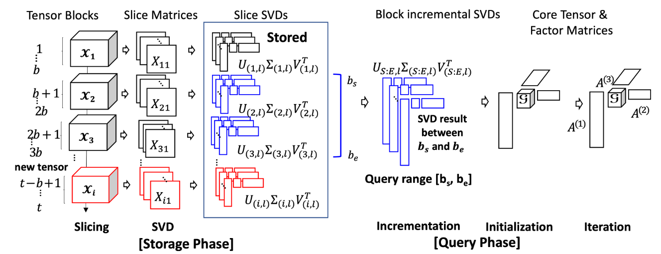
Our proposed Block Incremental Dense Tucker Decomposition (BID-Tucker) method efficiently stores and decomposes, on-demand, the multi-dimensional tensor data that are dynamically generated in the form of dense tensor blocks. Each incoming tensor block is transformed into slice matrices. Each of the slice matrices is then decomposed by a singular value decomposition (SVD) method. The approach of decomposing slice matrices was proposed in D-Tucker [12] for static tensors. We extend the approach to dynamically generated tensors. We store the block-wise SVD results of the slice matrices and use them, on-demand, to decompose the original tensor blocks (Fig. 1). Storing the SVD results instead of the original tensor blocks significantly reduces memory requirements. The Tucker decomposition result of the queried tensor blocks can be further analyzed and used for modeling. In this paper, we apply our method to spatiotemporal air quality tensor data and perform analysis to detect spatial and temporal trends.

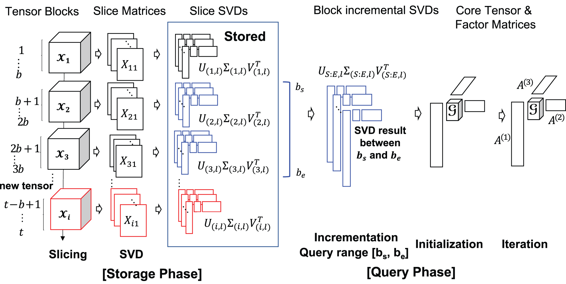
Figure 1: Storage phase and query phase of the proposed BID-TUCKER

Our contributions are summarized as follows:

•   Propose an efficient storage method for block-wise generated tensor stream data.

•   Propose an efficient on-demand dense tensor decomposition method for queried blocks for further analysis and modeling.

•   Compare the reconstruction error and the computational speed of the proposed method with D-Tucker [12] and vanilla Tucker decomposition.

•   Apply the proposed method to Korean air quality data and show how spatial and temporal trends can be modeled.

2  Background

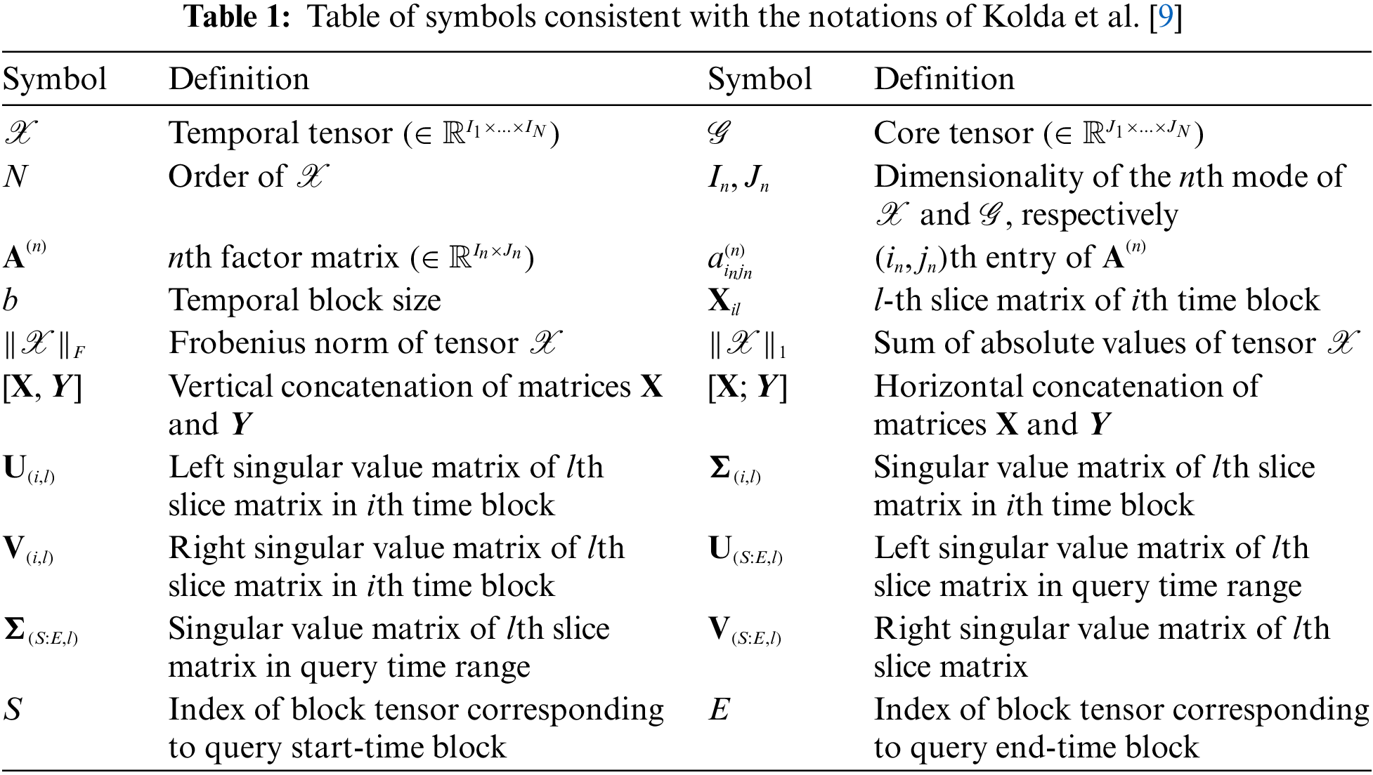
We begin by summarizing the tensor operation and the terms used in the paper. The notations and descriptions are consistent with the notations of Kolda et al. [9] and also D-Tucker [12]. Table 1 lists the symbols used.

2.1 Tensor Operation

Matricization transforms a tensor into a matrix. The mode-n matricization of a tensor X∈RI1×I2×⋯×IN is denoted as X(n). The mapping from an element (i1,...,iN) of X to an element (in,j) of X(n) is given as follows:

j=1+∑k=1,k≠nN[(ik−1)∏m=1,m≠nk−1Im].(1)

Given a tensor of the form X∈RI1×I2×I3⋯×IN, slice matrices are two-dimensional slices of the tensor defined by fixing all but two indices. For example, in a 3rdorder tensor, the horizontal, lateral, and frontal slices of the tensor X∈RI1×I2×I3 can be denoted as Xi1::, X:i2:, and X::i3, respectively. A mode-1 matrices X(1) of a tensor X can be represented as slice matrices as follows:

X(1)=[X::1;⋯;X::(I3×⋯×IN)]=[X1;⋯Xl;⋯XL],(2)

where Xl∈RI1×I2, L is equal to I3×⋯×IN, and the index l is defined using the following equation [9]:

l=1+∑i=1N((ki−1)∏m=3i−1Km),(3)

where Km is the dimensionality of mode-m, N is the order of the input tensor, and ∏m=3i−1Km equals 1 if i−1<m. Note that on the right hand side of the Eq. (2) there is a slice matrix Xl denoted by the index l.

N-mode product allows multiplications between a tensor and a matrix. The n-mode product of a tensor X∈RI1×⋯×IN with a matrix U∈RJn×In is denoted by X×nU. The resulting tensor has the shape of I1×⋯×In−1×Jn×In+1 ×⋯×IN. The element-wise n-mode product of a tensor can be written as follows:

(X×nU)i1⋯in−1jnin+1⋯iN=∑in=1In(Xi1i2⋯iNUjnin).(4)

For more on tensor operations, please refer to a review by Kolda et al. [9].

2.2 Block Incremental Singular Value Decomposition

Incremental singular value decomposition (incremental SVD) is a method that generates the SVD result of a growing matrix in an incremental manner. Let X consist of two vertically concatenated blocks XA and XB. Also, let Ui, Σi, and ViT be the SVD result of a given matrix i. We can compute the SVD of the vertically concatenated X as follows [13]:

X=[XAXB]≈[UAΣAVATUBΣBVBT]=[UAOOUB][ΣAVATΣBVBT]=[UAOOUB]U^Σ^V^T.(5)

With the above equation, the SVD result of X is as follows:

X=UΣVT where  U=[ UAOOUB ]  U^,Σ=Σ^,  and  VT=V^T.(6)

2.3 Tucker Decomposition

Our proposed method is based on one of the most popular tensor decomposition methods, the Tucker decomposition [9]. Tucker decomposition decomposes tensors into factor matrices of each mode and a core tensor. Given an nth order tensor X (∈RI1×...×IN), the Tucker decomposition approximates X to a core tensor G (∈RJ1×....×JN) and factor matrices {A(n)∈RIn×Jn|n=1...N}. The core tensor G is much smaller than the input tensor X and the factor matrices A(n) are normally column orthogonal. The Tucker decomposition with tensor operations is shown as follows:

X≈G×1A(1)⋯×NA(N).(7)

2.4 Higher-Order Orthogonal Iteration (HOOI) Algorithm

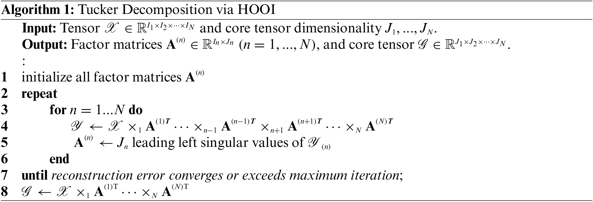
A widely used technique for minimizing the reconstruction error in a standard Tucker decomposition is alternating least squares (ALS) [9], which updates a single factor matrix or core tensor while holding all others fixed. Algorithm 1 describes a vanilla Tucker factorization algorithm based on ALS, called higher-order orthogonal iteration (HOOI) (see [9] for details). Algorithm 1 requires the storage of a full-density matrix Y(n), and the amount of memory needed to store Y(n) is O(In∏m≠nJm). Also, computing a single n-mode product between an input tensor X and the factor matrices A(n), as in Eq. (8), requires O(Jn∏m≠nIm) time complexity.

Y←X×1A(1)T⋯×n−1A(n−1)T×n+1A(n+1)T⋯×NA(N)T(8)

As the order, the mode dimensionality, or the rank of a tensor increases, the amount of memory required grows rapidly.

2.5 Sequentially Truncated HOSVD Algorithm

Sequentially Truncated Higher Order SVD (ST-HOSVD) [14] calculates the HOSVD in sequentially truncated form as follows in the Algorithm (2) using randomized SVD.

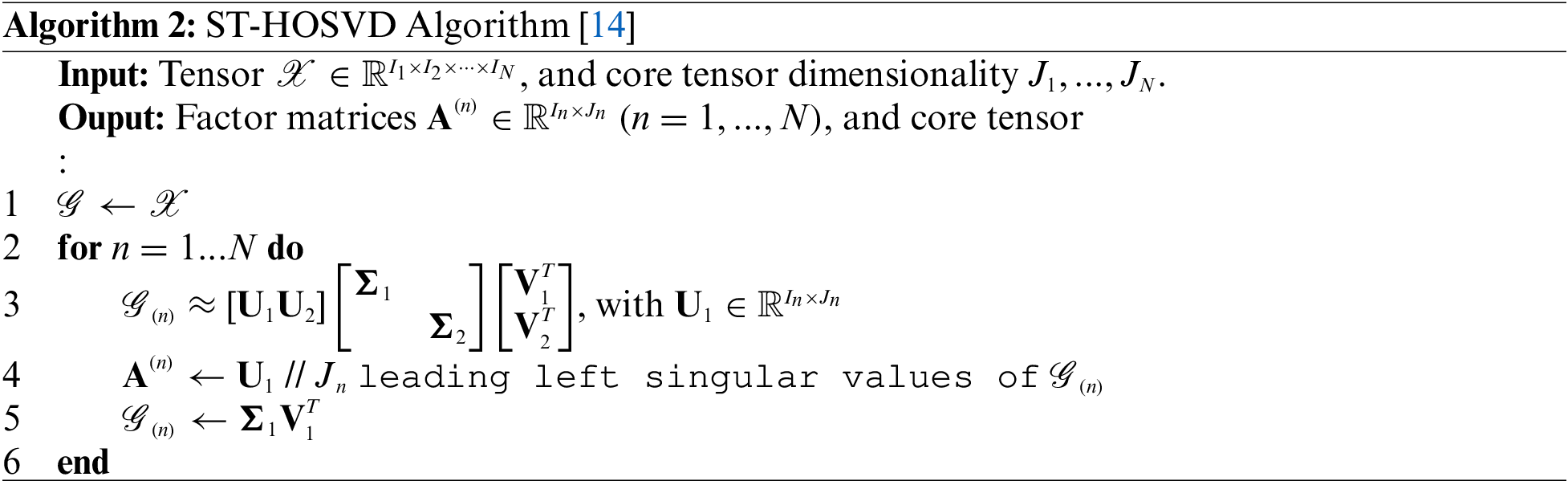
The ST-HOSVD algorithm provides a way to sequentially obtain factor matrices without the repeated mode-n products between the original tensor and all other factor matrices, as in line 4 of the Algorithm 1.

3  Block Incremental Dense Tucker Decomposition

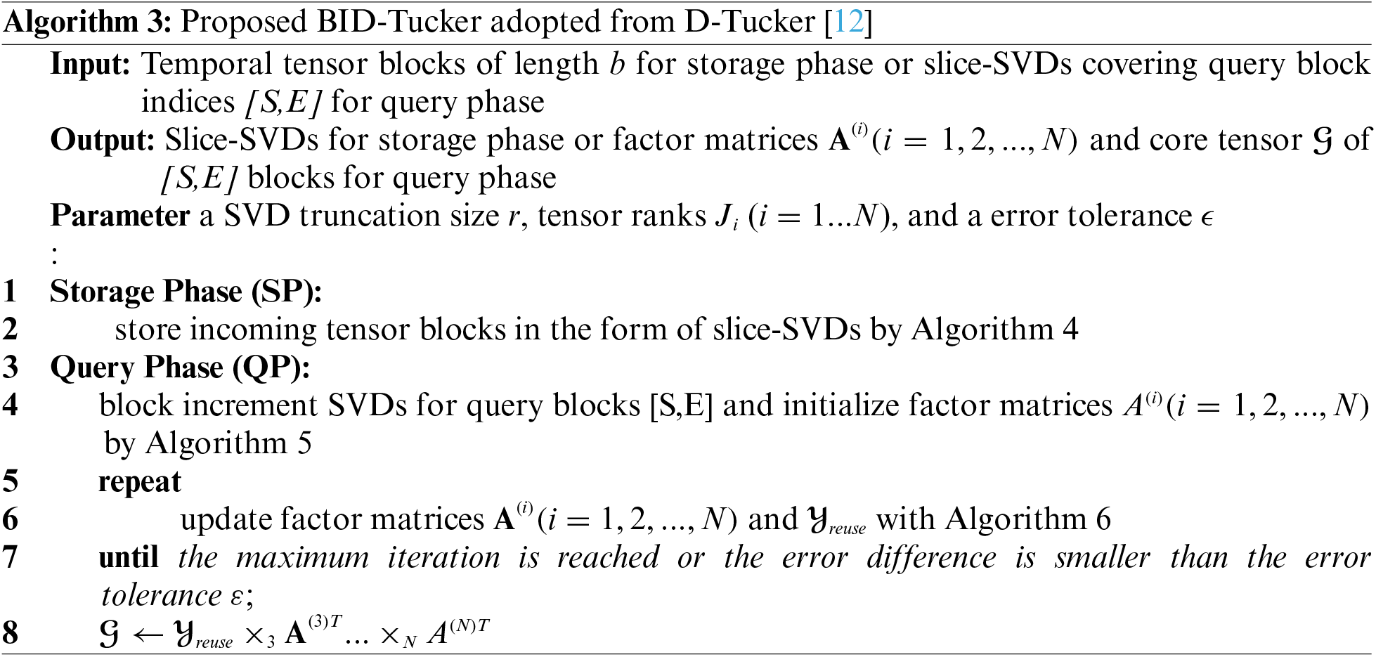
Our proposed Block Incremental Dense Tucker Decomposition (BID-Tucker) method assumes that only the time mode increases in dimension and dimensions remain for the rest of the modes. Our BID-Tucker is divided into two phases (Fig. 1 and Algorithm 3): the storage phase and the query phase. In the storage phase, incoming tensor blocks are stored as slice SVDs. The slice SVDs are then used in the query phase to efficiently decompose tensor blocks. In the query phase, a dense Tucker decomposition is performed on the user-specified query blocks. The decomposition results can be used for further analysis such as anomaly detection. We explain our approach for both phases in detail.

3.1 Storage Phase

Our storage phase, inspired by the block incremental SVD in FAST [13] and the approximation step of D-Tucker [12], provides a method to efficiently store the incoming tensor blocks. When a new tensor block arrives at the input system, the tensor is first sliced, where the two unfixed indices are time and space. Next, each of the sliced matrices is decomposed by the SVD. Only the SVD results are stored: singular values containing rectangular matrices Σs, left singular vector matrices Us, and right singular vector matrices Vs.

Assuming there are B blocks and the SVD truncation size is R, the space requirement is O(BI1RL), where I1 is the time mode dimension and L=I3×⋯×IN is the number of sliced matrices for the input tensor Xb∈I1×⋯×IN. If O(BI1RL) is small enough, they can be stored in memory. Otherwise, the SVD results can be stored on disk for later retrieval. For our experiments, we assume that the SVD results stored in memory are used in the query phase for Tucker decomposition and analysis.

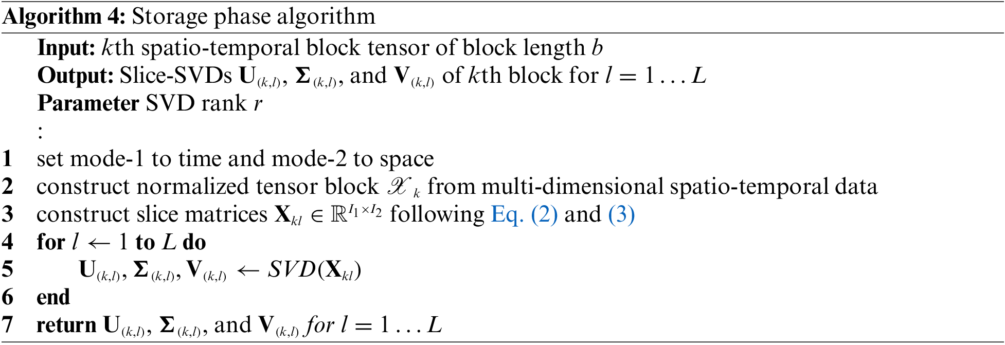
The storage phase is described in detail in the Algorithm 4. In the storage phase, given the spatiotemporal tensor data, the first mode is selected to be time, and the second mode is selected to be space (line 1). Once the two modes are selected, they are not changed during the storage and query phases. Afterward, the data is normalized so that all mode values are scaled, and a tensor is constructed (line 2). For each of the incoming tensor blocks, slice matrices are formed using the two modes, while the indices for the remaining modes are fixed (line 3). Each of the slice matrices is further decomposed with SVD, denoted as slice-SVDs (lines 4–6). Several SVD methods can be used. For smaller and less noisy tensor blocks, exact SVD can be used. For larger, noisy data, faster low-rank SVD methods such as randomized SVDs are recommended. Randomized SVDs are fast and memory efficient, and their low-rank approximation helps remove noise. Since most of the real-world sensor data is large and noisy, we used the randomized SVDs to generate the slice SVDs. We extend this process to each new incoming block of tensors. The process is shown in the storage phase of Fig. 1.

3.2 Query Phase

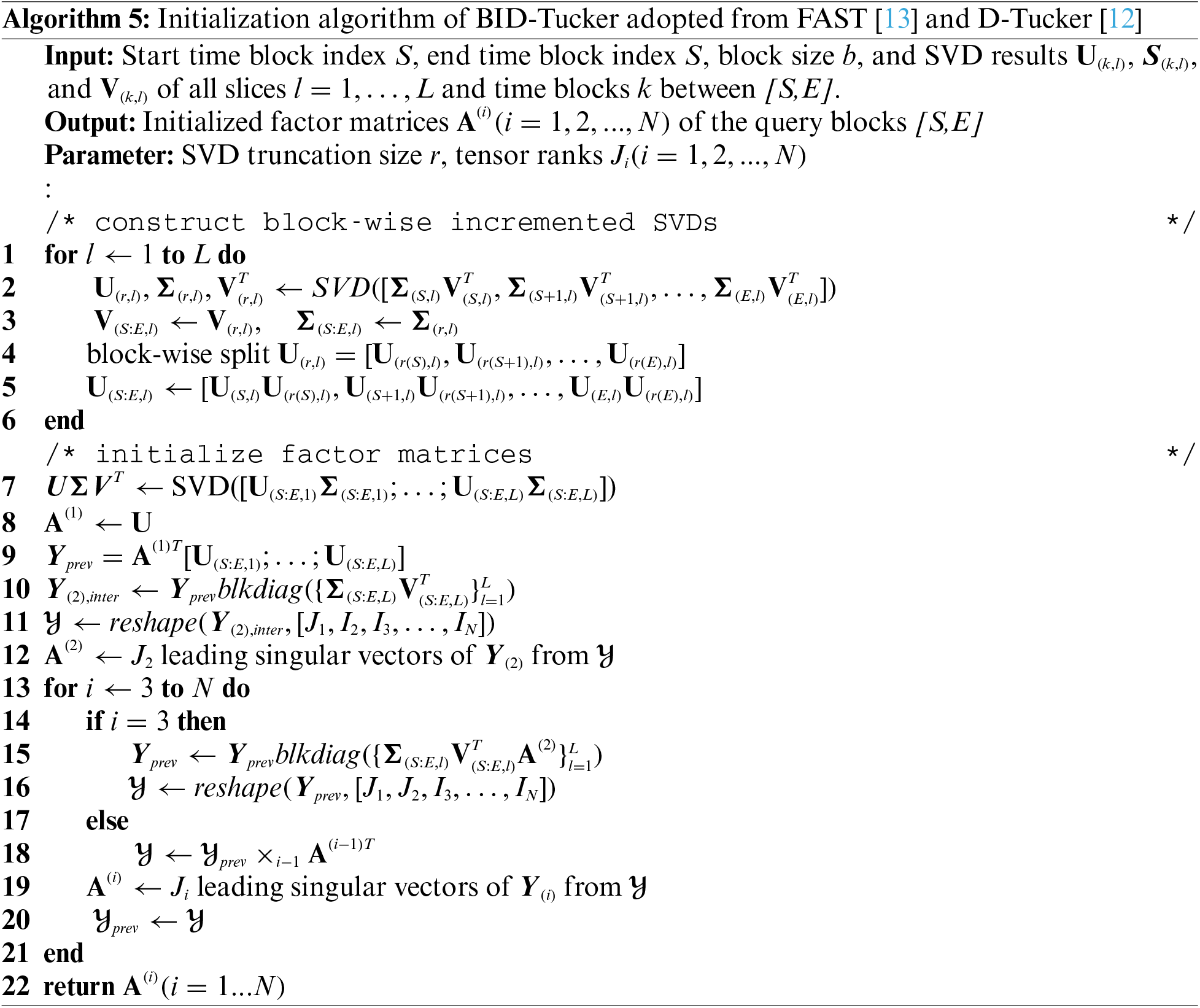
In the query phase, core tensor and factor matrices of the queried block tensors are generated on-demand. The stored slice SVDs of blocks in the query time range are retrieved and processed in two steps: initialization and iteration. First, BID-Tucker constructs a single slice-SVDs by block-wise incrementing the slice-SVDs of the requested time blocks [S, E], which are used to initialize the factor matrices. Our BID-Tucker then iterates over the factor matrices to find optimal cell values. The core tensor is computed after the last iteration.

3.2.1 Initialization

The left figure in the query phase of Fig. 1 shows the block-wise incremented SVDs and the initialization of our BID-Tucker. In the block-wise increment step, the block-wise slice-SVDs are used to generate slice-SVDs that cover the entire query blocks [S, E].

The specifics of block-wise incremented SVD are described in the following. Let [U(S,l);…;U(E,l)]; be the left singular vectors of the l-th slice matrix between the start block S and the end block E. All left singular vectors in the requested time blocks are concatenated into the block diagonal form as in Eq. (9).

blkdiag({Ul}l=SE)=[U(S,l)0…00U(S+1,l)0⋮⋱⋮0…0U(E,l)](9)

Then the l-th slice matrix corresponding to the time query blocks [S, E] is derived in the following:

X(S:E,i)≈[U(S,l)Σ(S,l)V(S,l)TU(S+1,l)Σ(S+1,l)V(S+1,l)T⋮U(E,il)′Σ(E,l)V(E,l)T]=blkdiag({U(b,l)}b=SE)[Σ(S,l)V(S,l)TΣ(S+1,l)V(S+1,l)T⋮Σ(E,l)V(E,l)T]=blkdiag({U(i,l)}i=SE)U(r,l)Σ(r,l)V(r,l)T=U(S:E,l)Σ(S:E,l)V(S:E,l)T.(10)

The [Σ(S,l)′V(S,l)′T;Σ(S+1,l)V(S+1,l)T;…;Σ(E,l)′V(E,l)′T] is decomposed and expressed as U(r,l), Σ(r,l), V(r,l)T (line 2). Singular value matrices and right singular vector matrices are assigned to be the newly decomposed values as in Σ(S:E,l)=Σ(r,l) and V(S:E,l)T=V(r,l)T (line 3). To update the left singular vector matrices, existing block diagonal matrices blkdiag({U(i,l)}i=SE) are multiplied by block-wise split U(r,l) matrices (line 4 and 5).

The next step in the initialization process is to initialize the cell values for the factor matrices and the core tensor of the query time range for efficient computation. There are two factors to consider when initializing. The first factor is that we do not want to refer to the original tensor values since we discard them after the storage phase. The second factor is that we want to initialize well so that the number of iterations required in the alternating least squares (ALS) procedure is minimal. D-Tucker [12] provides a way to decompose the tensor blocks with slice SVDs, which addresses both purposes. The method showed tolerable reconstruction error and a reduced number of iterations in ALS [12]. In fact, our factor matrix initialization and iteration steps follow the initialization and iteration phases of the D-Tucker [12], modified higher-order orthogonal iteration (HOOI) algorithm (Algorithm 1). We rewrite them here for clarity of the proposed BID-Tucker.

The computational bottleneck of naive HOOI is the computation of a single n-mode product between the input tensor X and the factor matrices (line 4 of Algorithm 1). Again, there are two problems with the naive HOOI approach: it requires the input tensor X and the space complexity is high. Fortunately, the input tensor X can be approximated with the stored slice SVDs for each block without reconstruction, which also improves the time and space complexity. This is possible by approximating the mode-n tensor with slice matrices and replacing the regular higher-order singular value decomposition (HOSVD) approach used in regular HOOI (lines 5 and 8 of Algorithm 1) with the sequentially truncated higher-order singular value decomposition (ST-HOSVD) [14] approach. ST-HOSVD sequentially assigns the truncated left singular vector matrix of the mode-n tensor as the mode-n factor matrix. first mode More specifically, the first mode factor matrix A(1) can be obtained by first representing the mode-1 tensor X(1) as follows:

X=X(1)=[X1;…;Xl;…;XL]≈[U1Σ1V1T;…;UlΣlVlT;…;ULΣLVLT]=[U1Σ1;…;UlΣl;…;ULΣL]×(blkdiag({VlT}l=1L))≈UΣVT(blkdiag({VlT}l=1L))(11)

where L is equal to I1×..×IN, l is as defined in Eq. (3), UΣVT is the SVD result of [U1Σ1; …; UlΣl; …; ULΣL], and blkdiag({VlT}l=1L) is the block diagonal form of right singular vectors Vls similar to Eq. (9). With the above mode-1 tensor X(1) representation and application of ST-HOSVD, we can obtain the initial factor matrix for the first mode as A(1)=U (line 8).

The initialization of the mode-2 factor matrix A(2) also follows the ST-HOSVD and respects the order of the tensor operations. As with the first mode factor matrix, A(2) is initialized to be the left singular vectors of the mode-2 matrices of X×1A(1), but without explicit reconstruction of X as in Eq. (12).

X×1A(1)T=A(1)TX(1)≈A(1)T[U1Σ1V1T;…;UlΣlVlT;…;ULΣLVLT]=(A(1)T[U1;…;Ul;…;UL])blkdiag({ΣlVlT}l=1L)=Y(2),interblkdiag({ΣlVlT}l=1L)(12)

where Y(2),inter= A(1)T[U1;…;Ul;…;UL], L is equal to I3×⋯×IN, blkdiag({ΣlVl}l=1L) is a block diagonal matrix. Transforming the right-most equation in Eq. (12) to RJ1×I2×⋯×IN and taking the left singular vectors from mode-2 matricized from gives the initial values for A(2) (lines 9–11).

Initialization of the mode-3 factor matrix A(3), following the ST-HOSVD, is also similar. As with the mode-1 and mode-2 factor matrice, A(3) is initialized to be the left singular vectors of mode-3 matricization of X×1A(1)×2A(2) again without explicit reconstruction of X as in Eq. (13).

X×1A(1)T×2A(2)T=A(1)TX(1)blkdiag({A(2)}l=1L)≈(A(1)T[U1;…;UL])blkdiag({ΣlVlTA(2)}l=1L)=Y(2),interblkdiag({ΣlVlTA(2)}l=1L)(13)

where Y(2),inter= A(1)T[U1;…;Ul;…;UL], L is equal to I3×⋯×IN, blkdiag({ΣlVl}l=1L) is a block diagonal matrix. Reshaping the rightmost equation in Eq. (13) to RJ1×J2×⋯×IN and taking left-singular vectors from mode-3 matricized from gets the initial values for A(3) (lines 15, 16, 19).

The remaining modes i=4,…,N following the ST-HOSVD can also be initialized by taking the left singular vectors of mode-i in the matricized form of X×1A(1)T×2A(2)T×i−1A(i−1)T (line 13). For efficient computation, D-Tucker [12] avoids redundant computation by finding the recursive computation pattern of Yprev×i−1A(i−1)T. That is, the recursive computation of Yprev to mode-3 (line 15) is just the mode-i−1 product between Yprev and A(i−1)T (line 18).

3.2.2 Iteration

After initialization, to reduce reconstruction error, ALS is performed over the factor matrices to generate optimal cell values for factor matrices A(i)(i=1...N). We follow the iteration procedure of the D-Tucker [12], which follows the HOOI iteration process that (1) approximates the original tensor X with stored SVD results (2) carefully arranges the update for the first- and the second-factor matrices by utilizing SVD results and their transpose (3) and avoid duplicate calculations of the intermediate tensor.

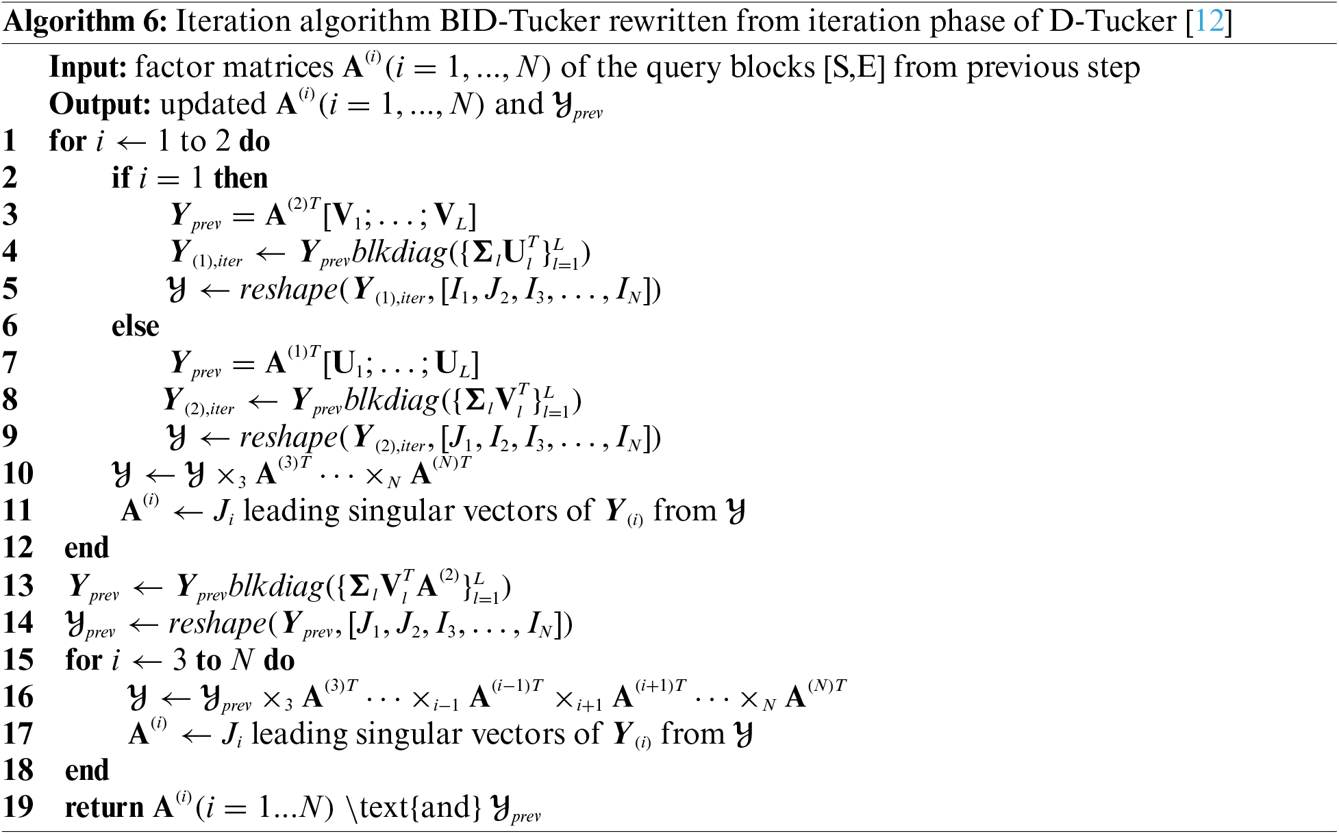
The overall ALS iteration process is shown in Algorithm 6, which we describe in detail. Again, the algorithm and description follow those of D-Tucker [12] which is an approximate form of the HOOI Algorithm 1. HOOI constructs an intermediate tensor that Y by n-mode products of the original tensor and the factor matrices, except for the factor matrix that is to be updated. D-Tucker approximates this process for the updated first-factor matrix by computing the approximate of X×2A(2)T with the previous factor matrix A(2)T and transposing the SVD of stitched matrices (lines 3–5). Then, the rest of the factor matrices are multiplied normally (line 10), prior to the factor matrix update (line 11). The second-factor matrix is updated similarly (lines 7–11). Prior to the update of the rest of the factor matrices, intermediate tensor Yprev that approximates X×1A(1)T×2A(2)T is calculated for repeated reuse (lines 13, 14). Then the algorithm follows the same procedure as the HOOI (lines 16–17). Standard SVD is used for finding the leading singular vector of Y(i) (lines 11, 17).

3.3 Complexity Analysis of BID-Tucker

To simplify the theoretical analysis of our BID-Tucker, we assume that the ranks of the output tensor are all J dimensional and that the dimensionality of a block of the input tensor is as follows: the dimension of the time mode is I and the dimension of remaining modes are all K, where I≤K≤J>0.

The storage phase takes O(BI2KN−2) time and O(BIRKN−2) space to process and store B blocks of the Nth order input tensor Xb∈I×K×⋯×K. Because the randomized SVD takes O(I12) [15] time, and the randomized SVD is performed on each of the L=KN−2 slice matrices for a block of the input tensor. The space requirement for the storage phase, given the SVD rank R, is O((IR+RR+KR)KN−2), since IR, RR, KR stand for the sizes of the left singular vectors, the singular values, and the right singular vectors of each of the KN−2 sliced matrices. The space complexity can be simplified to O(IRKN−2).

The query phase takes O(MNZIKN−2J2) time and O(ZIKN−2J) space, where I is the dimensionality of the input tensor, J is the output rank, Z is the number of tensor time blocks processed, M is the number of iterations, and N is the order of the input tensor. The query phase analysis of BID-Tucker largely follows the complexity analysis of D-Tucker, which takes O(IKN−2J2) time for initialization, O(MNIKN−2J2) time for iteration, and O(IKN−2J) space for processing a single block, B=Z=1, of the input tensor [12].

4  Anomaly Detection via Tensor Decomposition

After obtaining the core tensors and factor matrices of the desired time range [S, E], they can be used for spatial and temporal analysis. For the temporal analysis, we focus on finding unusual events. To do this, we define the anomaly score and the anomaly threshold based on the clusters of the time mode factor matrix. In a time mode factor matrix, a row contains latent values for the corresponding time point. Finding time-wise anomalies means finding unusual air quality that covers wide locations and features that differ from normal times.

The anomaly score: for each row of the time mode factor matrix is calculated by computing the minimum distance-to-centroid after clustering the row vectors. An appropriate clustering method can be selected after examining the distribution of the row vectors. We used k-means clustering but other clustering methods can be used. Then, for each cluster, a centroid vector ci∈C is constructed for i=1…K, where K is the number of clusters. Given a row vector v, the anomaly score is then defined as the distance of the vector to the nearest cluster. Specifically, we used the following score based on Euclidean distance:

as(v)=minci∈C||v−ci||2.(14)

Different distance measurements can be used.

The anomaly threshold can be selected, after calculating the anomaly scores, to detect unusual events. Since the distribution of distances follows the Gaussian distribution, we use unbiased estimates of the Gaussian distribution, i.e., the mean μ and the variance σ, to set the threshold. That is, the threshold T is calculated as the two standard deviations 2σ from the mean μ of the anomaly values as follows:

T=μ+Aσ.(15)

We set A=2 and consider events with a higher anomaly score than T to be unusual. However, to detect more extreme anomalies, a larger A value can be used.

5  Experiments and Results

We first describe our data set and the experimental setup. We then performed experiments to answer the following questions:

•   Ablation Study: How does the error change due to SVD truncation sizes and Tucker ranks in our proposed BID-Tucker?

•   Scalability Test: How scalable is our proposed method compared to D-Tucker and vanilla Tucker decomposition?

•   Application: What are the spatial and temporal properties of the air quality tensor that can be revealed by our proposed BID-Tucker?

5.1 Data Set and Experimental Setting

First, we describe the data preparation and experimental setup.

Air Quality Stream Data: We used Korean air quality data1 from 2018.01.01 to 2022.12.31 (41616-time points) to construct a 3rd-order temporal tensor for various spatial and temporal analyses. The Air Korea Air Quality Center measures and records particulate matter and air pollutants every hour from widely covered regions of South Korea, including remote islands. There are a total of 629 local monitoring stations with six types of measurements. The six types of measurements are ultrafine particulate matter (PM2.5; μgm2(1 h)), fine particulate matter (PM10; μgm2(1 h)), ozone (O3; parts per million (ppm)), nitrogen dioxide (NO2; ppm), carbon monoxide (CO; ppm), and sulfur dioxide (SO2; ppm).

Constructing Air Quality Tensor: After obtaining the raw air quality data, we constructed a spatiotemporal tensor.

First, a min-max normalization was performed for each measurement type after missing values were handled. Missing value handling is important in Tucker decomposition methods that use SVDs, where each input cell value is used to find the singular vectors and values. A small number of missing values can either be filled with zero or interpolated with mean values. When a large amount of data is missing. Then the resulting singular vectors and values may be misleading. Thus, for stations with less than 10% missing values, we filled the missing values with the average value of the corresponding normalized air quality measurement type for the corresponding station. Stations with more than 10% missing values were removed, leaving 316 stations.

We then constructed a 3rd order tensor, where the modes are (time,location,type). Overall, the shape of the obtained (time,location,type) indexed air quality tensor was (41616,316,6). In the experiment, we assumed that the tensor blocks are generated weekly for each hour (7∗24=168), so the incoming blocks were set to tensors with a shape of (168,316,6).

Experiment Settings: The study was conducted on a 12-core Intel(R) Core(TM) i7-6850K CPU @ 3.60 GHz. The following libraries were used with Python version 3.10: NumPy version 1.23.5, scikit-learn version 1.2.1, Pytorch 2.0.0, and Tensorly 0.8.1.

5.2 Ablation Study

There are two hyperparameters in the BID-Tucker: SVD truncation size and Tucker ranks. In the first ablation study, the SVD truncation size was varied and the corresponding normalized reconstruction error was measured to observe the effect of the SVD truncation size on the overall reconstruction error. In the second ablation study, Tucker ranks were varied, and normalized reconstruction errors were measured to evaluate the effect of rank sizes on overall reconstruction error. The normalized reconstruction error was calculated as ||Xorg−Xrecon||F/||Xorg||F. Again, we assumed that the air quality tensor of (41616,316,6) comes in a tensor stream of the form (168,316,6).

Fig. 2 (left) in the blue straight line shows the normalized reconstruction error as the SVD truncation sizes increase from 5 to 50 in the storage phase of the proposed BID-Tucker. In this test, the Tucker rank was set at (30,30,6). The normalized error started to decrease slowly after the size of 20. Unless otherwise specified, the SVD truncation size was set to 20 in the remaining experiments.

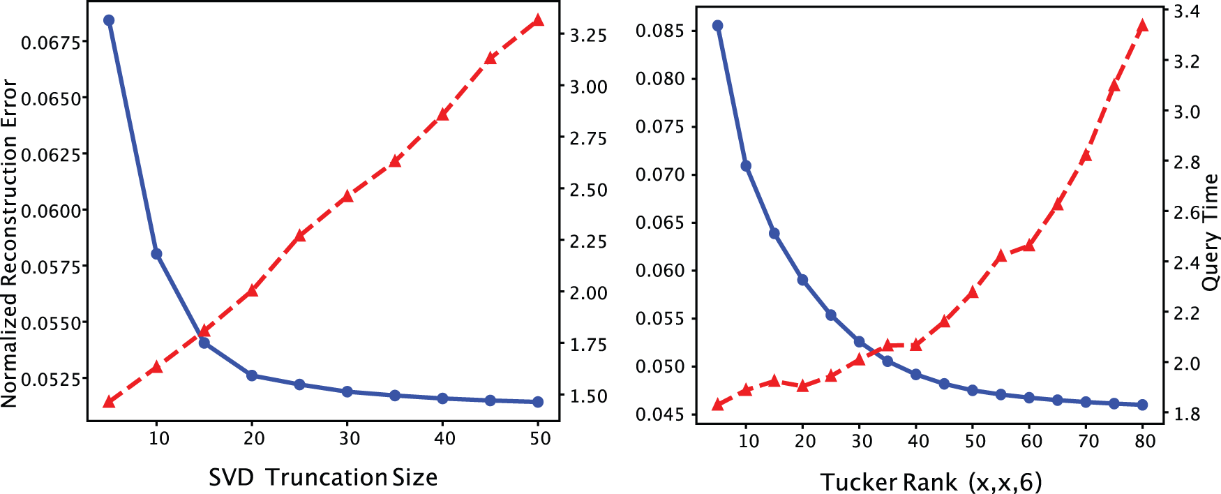
Figure 2: Normalized reconstruction error in blue solid lines and query processing time in red dotted lines over SVD truncation size with tensor ranks (30,30,6) (left) and tensor rank in the form of (x, x, 6) with SVD truncation size 20 (right)

The Fig. 2 (right) in the blue straight line shows the normalized reconstruction error for different Tucker rank tuples. The tensor ranks for the time and location modes were set equal. The rank for the type mode was set to 6. The ranks were varied from (5,5,6) to (80,80,6) in increments of 5. A rank size of 30 showed a low error for the air quality tensor. Unless otherwise specified, the Tucker ranks were set to (30,30,6) in the remaining experiments.

5.3 Scalability Test

In the scalability test, we first tested the scalability according to the SVD truncation size and the Tucker rank. Fig. 2 (left) in the red dotted lines shows the query processing time as the SVD truncation sizes increase from 5 to 50. The time complexity increased linearly as the SVD truncation size increased. Fig. 2 (right) in the red dotted lines shows the query processing time for different Tucker ranks. The Tucker ranks for the time and location modes were set equal, and the rank for the type modes was set to 6. The ranks were varied from (5,5,6) to (80,80,6), increasing by 5. The processing time increased in a near quadratic form which is also evident from the complexity analysis (Section 3.3) that shows the complexity to be proportional to the J2 where J is the Tucker rank.

In the second part of the scalability test, we answer the question of how scalable our proposed BID-Tucker is compared to D-Tucker and regular Tucker decomposition. We varied the input tensor sizes and computed the error and query processing time for the proposed BID-Tucker, D-Tucker, and HOOI-based vanilla Tucker decomposition. Fig. 3 shows the normalized reconstruction error on the left and the query processing time on the right. We can see from the left plot that all three methods have similar reconstruction errors. However, as we can see from Fig. 3 (left) that the error differences are small, less than 0.001. With the comparable loss, we then looked at how scalable each method is to the size of the input tensor.

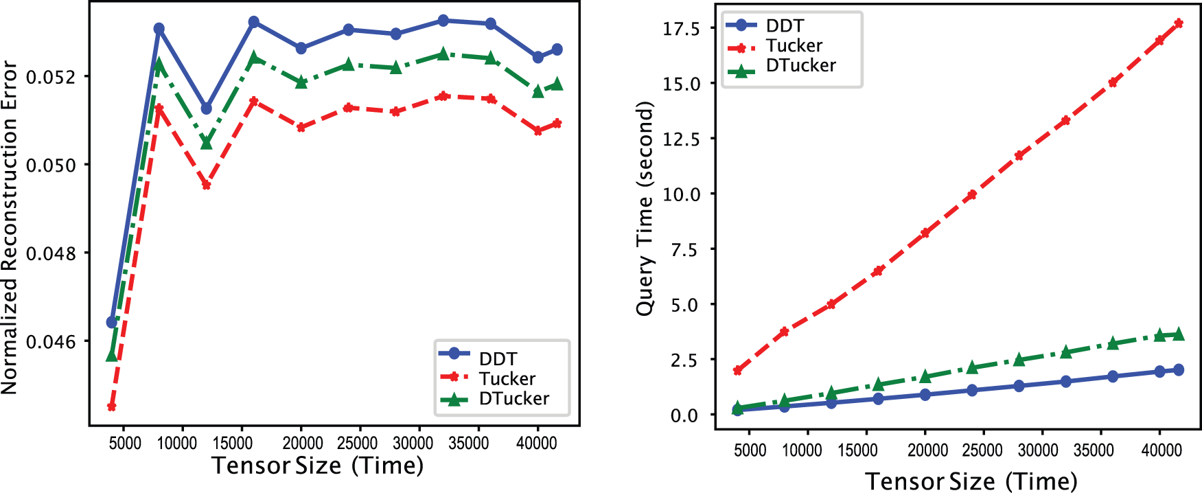
Figure 3: Comparison of normalized reconstruction error (left) and query processing time (right) of dynamically dense tucker decomposition (DDT) with D-tucker and HOOI-based vanilla tucker decomposition over different tensor sizes. The x axis is the length of the time mode for the input tensor, where the location mode dimension is fixed to 316 and the type mode dimension is fixed to 6

For a fair comparison, we included the processing time for both the storage and query phases and set the query range to the full range for our BID-Tucker. Fig. 3 (right) shows that our proposed BID-Tucker significantly outperformed vanilla Tucker and showed a lower growth rate compared to D-Tucker. The lower growth rate compared to D-Tucker comes from efficiency grained by block incremental SVD used in the storage phase.

Overall, our proposed method scales better than the compared methods, with a tolerable error difference.

5.4 Modeling Annual Trends of Korean Air Quality

We describe our analysis results for the Korean air quality data. First, we used the time mode factor matrix to experiment with whether we could detect unusual air quality. Then, we analyzed whether our method could detect regional similarities in air quality by analyzing the location mode factor matrix.

Temporal Modeling and Anomaly Detection: We clustered the time mode factor matrix of the decomposed air quality tensor for modeling the temporal trends and detecting unusual air quality events in Korean air quality. Specifically, we used the time mode factor matrix AT∈R(41616×30) over the entire data period from the year 2018 to 2022 over the latent dimensions to perform k-means clustering. The optimal k=3 was found by the elbow method, which plots the within-cluster sum of squares (WCSS) against the cluster size k (Fig. 4 (left)). Fig. 4 (right) shows the clustering result visualized by t-SNE (t-distributed stochastic neighbor embedding), where each color corresponds to a cluster.

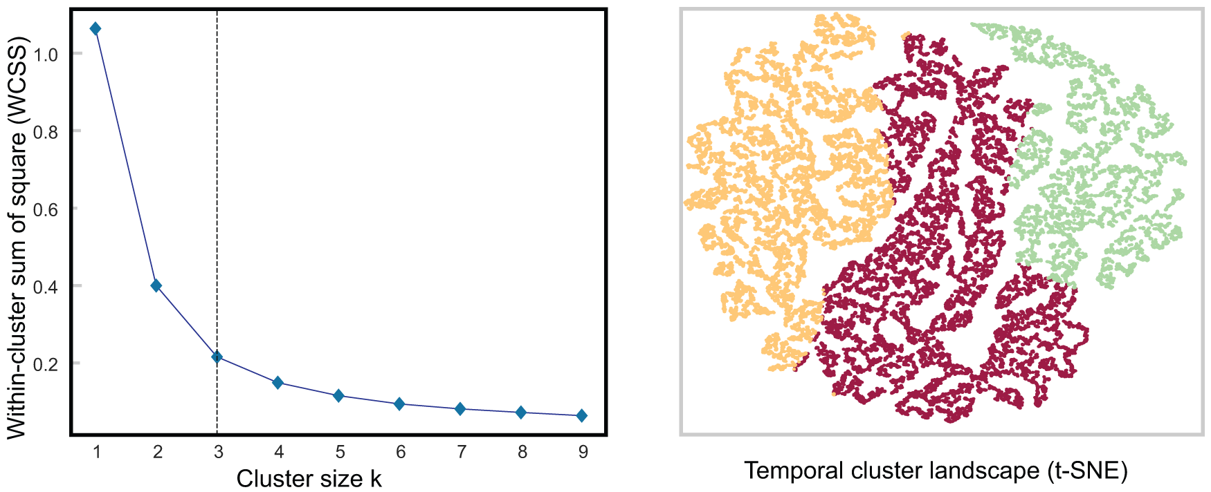
Figure 4: Temporal analysis of air quality data using k-means. The elbow method is used and plotted on the left to find optimal clusters of size three, the color-coded cluster distribution is plotted using t-SNE on the right

The three clusters map well to Korea’s four seasons, each of which has its own characteristics. Specifically, Cluster 1 (yellow) maps mainly to summer periods when temperatures and humidity are high nationwide. Ozone alerts are often issued during this time. Cluster 2 (red) mostly maps to the spring and fall seasons. Yellow dust and fine particle alerts are common during this time. Cluster 3 (purple) was mainly associated with the winter seasons. This period is characterized by cold, dry weather across the country, with occasional fine particle alerts.

To detect unusual air quality over time, we calculated anomaly scores as described in Section 4 using the Euclidean distance to the nearest cluster centroid of the time mode factor matrix. We considered anomaly scores above the mean +2×standard deviation to be unusual events. The vertical line in Fig. 5 corresponds to the threshold. We took a closer look at some of the unusual time points to see if there were any notable events in the news that could have led to the time point having a high anomaly score.

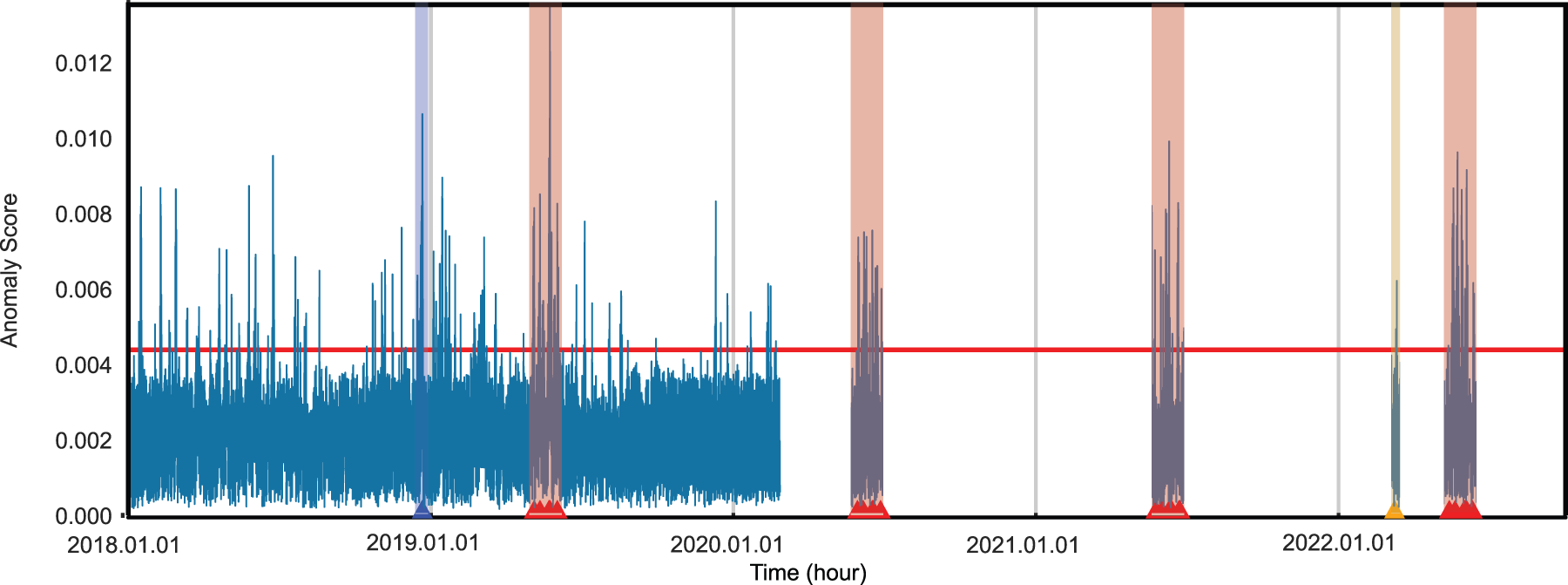
Figure 5: Temporal anomaly score plot with threshold and selected events. The x axis is the time points in chronological order from 2018-01-01 to 2022-12-31. The vertical line is the threshold at t=mean+2×standarddeviation. Red marks denote chronic high ozone concentration events. Blue marks denote the two construction fire events. Organ marks denote several forest fire events

We found two interesting items, chronic ozone alerts issued during the late spring and early summer periods and large fire events. The period from May to August between the years 2019 to 2022 contains several days with unusually high ozone levels2 . The time of high ozone concentration was between 13:00 and 17:00. The high ozone concentration during these periods occurred between 13:00 and 17:00, and the concentrations were two to three times higher than on normal days. These chronic events are marked in red in Fig. 5.

For fire events, we found several. Two marked cases are as follows: large construction fires and forest fire events. On December 28, 2018, there were two construction fires: the Jeonbuk sewage treatment plant fire on 2018-12-28 between 7:00 and 8:00, and the Busan factory fire on 2018-12-28 between 1:00 and 3:00. The anomaly values mean the effect of the fires on air quality lasted for a few days after the events. These events are marked in blue in Fig. 5. We also confirmed that large forest fires were detectable by the anomaly values. During the period from March 04, 2022 to March 11, 2022, there were several small and large fire events throughout the east coast of South Korea. The forest fire events are marked in orange in Fig. 5.

In addition, Fig. 5 shows that there is a difference in the pattern of anomaly values before and after the COVID-19 pandemic break. Before the pandemic break in December 2019, there were much more high peaks of anomaly air quality than during the pandemic. We speculate that this is related to the decrease in factory and vehicle utilization rates in and around nations during the pandemic.

Spatial Modeling: For the spatial modeling based on the air quality tensor, we performed K-means clustering on the location mode factor matrix AL∈R316×30. Similar to the temporal analysis, we selected the optimal k=3 using the elbow method (Fig. 6a) and visualized the clustering result using t-SNE (Fig. 6b).

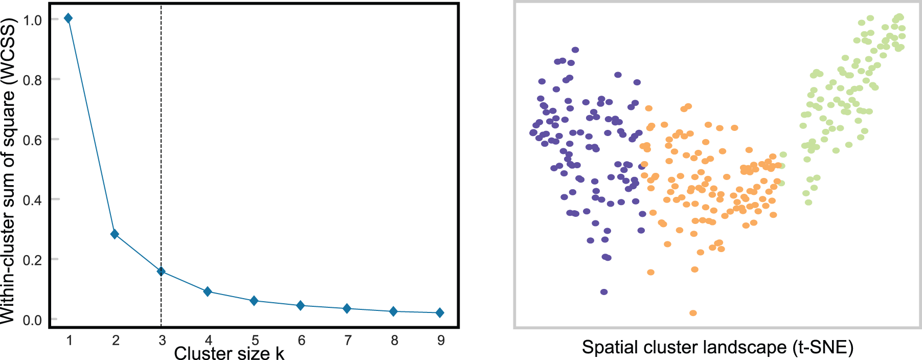
Figure 6: Spatial analysis of air quality data using k-means. The elbow method is used and plotted on the left to find optimal clusters of size three, the color-coded cluster distribution is plotted using t-SNE on the right

For each of the three clusters, we found distinct local similarities, which we list below. Cluster 1 (yellow) corresponded to the metropolitan areas, including Seoul and Incheon. Cluster 2 (purple) corresponded to the eastern half of South Korea, which is known to have better overall air quality throughout the year. The eastern half is mostly mountainous. Cluster 3 (red) corresponded to the western half of South Korea, which is known to have poor overall air quality compared to the eastern half, even in rural areas. The western half has fewer mountains and more plains.

6  Conclusion

Recognizing the need for efficient storage of spatiotemporal stream data in dynamic modeling, we proposed Block Incremental Dense Tucker Decomposition (BID-Tucker), which can provide efficient storage and on-demand Tucker decomposition results. Our BID-Tucker can be applied to any tensor data that comes in tensor blocks where the dimensions of modes stay the same except for the time mode. We also assume only partial time-ranged data needs to be analyzed and modeled. Our BID-Tucker stores the singular value decomposition (SVD) results of each sliced matrix of a tensor block instead of the original tensor. The SVD results of each time block are concatenated by block incremental SVD [13] and used to initialize the Tucker decomposition [12]. We have applied our BID-Tucker to the Korean Air Quality data for modeling the air quality trends. When applying it to the air quality tensor, we provided an approach to find the optimal SVD truncation size and Tucker rank. We used the same optimal setting to compare and show benefits in the error rate and scalability of our BID-Tucker to that of D-Tucker, which is an efficient Tucker decomposition method that our BID-Tucker extends, and the vanilla Tucker method, which is known to give the best error although not efficient. We further applied our BID-Tucker on the air quality tensor to model the air quality trends and detect unusual events. Also, we were able to verify that there are spatial similarities in the air qualities. Overall, we conclude that our proposed BID-Tucker was able to provide efficient storage and Tucker decomposition results on-demand for time block tensors. Although we only applied the BID-Tucker to the air quality tensor, it can be applied to various multi-dimensional spatiotemporal data, and the post-decomposition analysis process can be used for modeling spatial and temporal trends.

Acknowledgement: The authors wish to express their appreciation to the reviewers for their helpful suggestions which greatly improved the presentation of this paper.

Funding Statement: This work was supported by the Institute of Information & Communications Technology Planning & Evaluation (IITP) grant funded by the Korean government (MSIT) (No. 2022-0-00369) and by the National Research Foundation of Korea Grant funded by the Korean government (2018R1A5A1060031, 2022R1F1A1065664).

Author Contributions: The authors confirm their contribution to the paper as follows: study conception and design: S. Lee, L. Sael; data collection: H. Moon; analysis and interpretation of results: S. Lee, H. Moon, L. Sael; draft manuscript preparation: S. Lee, H. Moon, L. Sael. All authors reviewed the results and approved the final version of the manuscript.

Availability of Data and Materials: The Korean Air Quality Data has been obtained through the Air Korea Insitute portal at https://www.airkorea.or.kr/. Our codes for BID-Tucker and D-Tucker, written in Python, are provided in the GitHub https://github.com/Ajou-DILab/BID-Tucker.

Conflicts of Interest: The authors declare that they have no conflicts of interest to report regarding the present study.

1https://www.airkorea.or.kr/

2List of days and times of ozone alerts issued: 2019-05-23 25, 2019-06-19 21, 2019-08-02 05, 2019-08-18 20, 2020-06-06 09, 2020-07-16 17, 2020-08-18 21, 2021-05-13 19, 2021-06-05 09, 2021-06-20 25, 2021-07-20 24, 2022-05-23 25, 2022-06-20 22, 2022-07-10 16, 2022-07-25 26.

References

1. Jeon, I., Papalexakis, E. E., Kang, U., Faloutsos, C. (2015). HaTen2: Billion-scale tensor decompositions. Proceedings of the 31st IEEE International Conference on Data Engineering, Seoul, South Korea, IEEE. [Google Scholar]

2. Park, N., Jeon, B., Lee, J., Kang, U. (2016). Bigtensor: Mining billion-scale tensor made easy. Proceedings of the 25th ACM International on Conference on Information and Knowledge Management, Indianapolis, IN, USA. [Google Scholar]

3. Choi, D., Jang, J. G., Kang, U. (2019). S3CMTF: Fast, accurate, and scalable method for incomplete coupled matrix-tensor factorization. PLoS One, 14(6), 1–20. [Google Scholar]

4. Jang, J. G., Moonjeong Park, J. L., Sael, L. (2022). Large-scale tucker tensor factorization for sparse and accurate decomposition. Journal of Supercomputing, 78, 17992–18022. [Google Scholar]

5. Gujral, E., Pasricha, R., Papalexakis, E. E. (2018). Sambaten: Sampling-based batch incremental tensor decomposition. Proceedings of the 2018 SIAM International Conference on Data Mining, San Diego, California, USA. [Google Scholar]

6. Kwon, T., Park, I., Lee, D., Shin, K. (2021). Slicenstitch: Continuous cp decomposition of sparse tensor streams. 2021 IEEE 37th International Conference on Data Engineering (ICDE), Chania, Greece, IEEE. [Google Scholar]

7. Smith, S., Huang, K., Sidiropoulos, N. D., Karypis, G. (2018). Streaming tensor factorization for infinite data sources. Proceedings of the 2018 SIAM International Conference on Data Mining, San Diego, CA, USA. [Google Scholar]

8. Zhou, S., Vinh, N. X., Bailey, J., Jia, Y., Davidson, I. (2016). Accelerating online cp decompositions for higher order tensors. Proceedings of the 22nd ACM SIGKDD International Conference on Knowledge Discovery and Data Mining, San Francisco, CA, USA. [Google Scholar]

9. Kolda, T. G., Bader, B. W. (2009). Tensor decompositions and applications. SIAM Review, 51(3), 455–500. [Google Scholar]

10. Chachlakis, D. G., Dhanaraj, M., Prater-Bennette, A., Markopoulos, P. P. (2021). Dynamic l1-norm tucker tensor decomposition. IEEE Journal of Selected Topics in Signal Processing, 15(3), 587–602. [Google Scholar]

11. Jang, J. G., Kang, U. (2023). Static and streaming tucker decomposition for dense tensors. ACM Transactions on Knowledge Discovery from Data, 17(5), 1–34. [Google Scholar]

12. Jang, J. G., Kang, U. (2020). D-tucker: Fast and memory-efficient tucker decomposition for dense tensors. 2020 IEEE 36th International Conference on Data Engineering (ICDE), Dallas, Texas, USA. [Google Scholar]

13. Jinhong Jung, L. S. (2020). Fast and accurate pseudoinverse with sparse matrix reordering and incremental approach. Machine Learning, 109, 2333–2347. [Google Scholar]

14. Vannieuwenhoven, N., Vandebril, R., Meerbergen, K. (2012). A new truncation strategy for the higher-order singular value decomposition. SIAM Journal on Scientific Computing, 34(2), A1027–A1052. [Google Scholar]

15. Woolfe, F., Liberty, E., Rokhlin, V., Tygert, M. (2008). A fast randomized algorithm for the approximation of matrices. Applied and Computational Harmonic Analysis, 25(3), 335–366. [Google Scholar]