
 Submit a Paper
 Propose a Special lssue
 Open Access
ARTICLE

RB-DEM Modeling and Simulation of Non-Persisting Rough Open Joints Based on the IFS-Enhanced Method
1 Key Laboratory of Ministry of Education for Geomechanics and Embankment Engineering, Hohai University, Nanjing, 210098, China
2 Research Institute of Geotechnical Engineering, Hohai University, Nanjing, 210098, China
3 School of Earth Sciences and Engineering, Hohai University, Nanjing, 210098, China
4 State Key Laboratory for Geomechanics and Deep Underground Engineering, China University of Mining and Technology, Xuzhou, 221116, China
* Corresponding Author: Qingxiang Meng. Email:
Computer Modeling in Engineering & Sciences 2024, 139(1), 337-359. https://doi.org/10.32604/cmes.2023.031496
Received 21 June 2023; Accepted 22 September 2023; Issue published 30 December 2023
 View Full Text
 Download PDF
Abstract
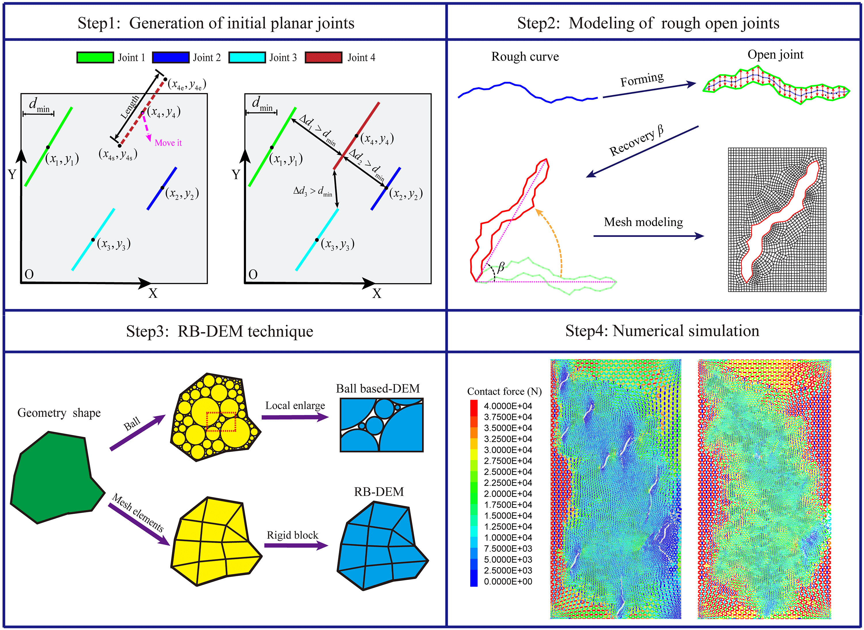
When the geological environment of rock masses is disturbed, numerous non-persisting open joints can appear within it. It is crucial to investigate the effect of open joints on the mechanical properties of rock mass. However, it has been challenging to generate realistic open joints in traditional experimental tests and numerical simulations. This paper presents a novel solution to solve the problem. By utilizing the stochastic distribution of joints and an enhanced-fractal interpolation system (IFS) method, rough curves with any orientation can be generated. The Douglas-Peucker algorithm is then applied to simplify these curves by removing unnecessary points while preserving their fundamental shape. Subsequently, open joints are created by connecting points that move to both sides of rough curves based on the aperture distribution. Mesh modeling is performed to construct the final mesh model. Finally, the RB-DEM method is applied to transform the mesh model into a discrete element model containing geometric information about these open joints. Furthermore, this study explores the impacts of rough open joint orientation, aperture, and number on rock fracture mechanics. This method provides a realistic and effective approach for modeling and simulating these non-persisting open joints.Graphic Abstract
Keywords
Rock masses, as natural geological formations, contain numerous non-persistent rough closed joints, which result in their mechanical properties being very complicated [1]. When human activities are carried out, such as the excavation of foundation pits that can disrupt the initial stress state of surrounding rock, closed joints could be transformed to open joints [2], as illustrated in Figs. 1a–1c. This can further weaken the pressure-bearing capacity of the rock mass. However, the influence on the surrounding rock is unavoidable due to engineering needs. Hence, investigating these open joints on the mechanical behavior of rock masses also holds great significance.
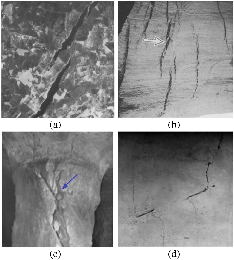
Figure 1: Failure of rock mass caused by pre-existing joints: (a) and (b) tensile fractures in potash salt rock [11]; (c) coalescence of open joints [12]; (d) two open joints in rock-like materials [7]
The current research on jointed rock is divided into two main types, containing physical and simulation experiments. In physical experiments, it is further classified into tests on natural rocks and artificial samples. In-situ survey experiments can get natural rock mass from the drill, where key data such as the orientation, size, and geometry of joints are obtained [3–5]. However, obtaining an undisturbed rock mass is exceedingly difficult, as drilling inevitably disturbs joints within the surrounding rock, leading to changes in the collected data [6]. The preparation of rock-like samples with pre-existing open flaws (the term ‘flaw’ denotes an artificial joint) has gained great popularity and has been conducted by multiple scholars. Cao et al. prepared and tested brittle materials containing two pre-existing open joints [7]. Chen et al. analyzed the deformation behavior of jointed rock masses for gypsum specimens experimentally [8]. In uniaxial compression, Lee et al. examined the coalescence of fractures on jointed specimens with different orientations [9]. Yang et al. studied the strength failure and crack coalescence behavior of sandstone containing 3 pre-existing open joints [10].
According to these experimental tests, new cracks can be divided into two types based on the failure mode: wing cracks and secondary cracks [7]. Wing cracks, also known as primary cracks, result from the tension that originates from the tips of pre-existing flaws and propagates in the direction of maximum compressive stress [13]. On the other hand, secondary cracks are shear cracks that exhibit a surface characterized by pulverized material and a very rough texture with crushed material [14]. Although some findings were achieved through the study of artificial samples, they often contain only a few open joints, as shown in Fig. 1d. The stochastic distribution of joints is very complex, such as Poisson-, Gaussian- and lognormal distribution [15]. It is challenging to prepare rock mass samples containing complex distributed flaws [16]. Furthermore, the experimental results are highly dependent on the sample preparation process as well as the boundary loading conditions. Even minor changes in the contact conditions between specimens and the loading plate can lead to different failure modes [17].
With the remarkable advancement in computer performance, several numerical methods were developed to simulate the effect of open joints on the mechanical behavior of rock masses. These methods can be mainly classified into two categories: continuous and discontinuous methods. The former includes the finite element method (FEM) and finite difference method (FDM) [18,19]. Due to the discontinuity of rock masses, discontinuous methods are more advantageous than the other one, which has become a powerful tool for studying these rock masses. Discontinuous methods include the discontinuity deformation analysis (DDA) [20] and the discrete element method (DEM) [21]. Due to the unique advantage of being able to represent the displacement, rotation, and motion of all discrete elements, the DEM has become a popular tool for analyzing rock behavior [22]. Under uniaxial compressive loading, Zhang et al. analyzed crack initiation and propagation [23]. Cao et al. simulated the failure behavior of a multi-joint specimen using the PFC2D, which is a DEM software [24]. Based on the numerical direct shear test, Sarfarazi et al. investigated the impact of joint overlap on the failure process [25]. Nonetheless, two-dimensional (2D) DEM numerical simulations still have two severe disadvantages. First, open flaws are usually treated as planar joints with a constant aperture, which cannot represent real open joints. The second drawback is that the basic discrete element is often represented by disk-shaped particles (the ball) with many micro-voids between them, and it is almost impossible to accurately show the geometric features of rough joints.
In response to the first defect, some scholars suggested that the jointed rock has a fractal structure [26]. The fractal interpolation system (IFS) [27] can be used to generate rough closed joints based on polylines with low orientation, such as Yang et al. who constructed a finite element mesh containing a single fractal joint [28]. However, as for planar lines, or polylines with high inclination, IFS still fail to handle them. In addition, there is no certain method to generate relatively realistic rough surfaces for open joints. Regarding the second problem, the situation has recently improved with the introduction of the Rigid Block Discrete Element Method (RB-DEM) proposed by Meng et al. [29]. In RB-DEM, the rigid block (rblock) is selected as the basic discrete element and each one is converted from a finite element mesh, providing a more realistic representation than traditional ball-based discrete elements.
With this in mind, a new solution is proposed in this paper to generate discrete element models with realistic non-persisting open joints. Based on the stochastic distribution of joints and an enhanced IFS method that can deal with planar lines and polylines with any orientations, rough curves can be generated. Then, the Douglas-Peucker algorithm [30] is used for the simplification of these curves while maintaining its fundamental shape to delete some unnecessary points that can lead to some distorted mesh elements. Next, points on the rough curve except for the two ends, are moved to both sides according to the joint aperture distribution law. These points are connected with the start and end points to form an open joint, followed by mesh modeling software to build the finite mesh model. Finally, the finite element model with geometric features of these joints is constructed, and use the RB-DEM to convert the model to a discrete element model. The mechanical parameters obtained based on the pairwise algorithm [31] are used to analyze the effect of open joints on crack development. In addition, the effects of orientation, aperture, and density of rough joints on the fracture behavior of rock mass are also discussed. This work presents a more realistic and efficient tool for the modeling and simulation of non-persisting open joints.
2.1 Generation of Initial Planar Joints
2.1.1 Stochastic Distribution of Joints
It is limited to the use of artificial specimens containing only a single set of joints to predict the mechanical behavior of rock mass containing numerous random joints. In recent years, numerical modeling of rock masses with stochastically distributed no-persistent joints has been popular among scholars and discrete fracture network (DFN) is an effective tool [32–35]. Geometrical parameters of a set of joints include position, aperture, length, and orientation. In this study, the spatial distribution of joints is set as a relatively random distribution by controlling the minimum distance (
where
where
To generate joints of varying lengths and positions, besides the above statistical distribution, the following two judgment conditions are also needed to be satisfied. Firstly, after setting the boundary of the rock mass model, a point is selected randomly inside the model, which is taken as the midpoint of the single joint. The start and end points of the joint are determined based on the length and orientation distribution pattern. Verify whether the start and end points are beyond the boundary and if so, move it until the start and end points are within the model, as shown in Fig. 2a. Subsequently, compute the distance (
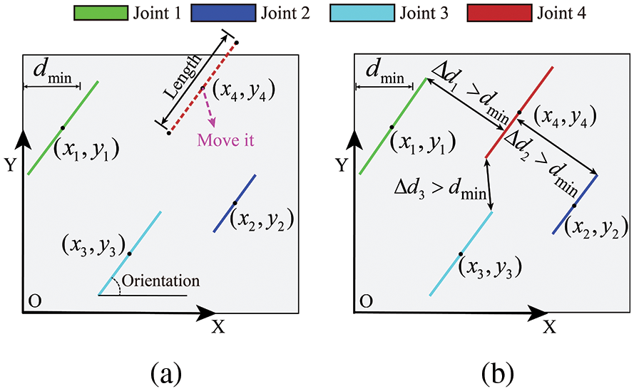
Figure 2: Illustration of initial planar joints generation and movement: (a) generation; (b) movement
2.2 Enhanced Fractal Interpolation System
2.2.1 Polyline Generation and Orientation Rotation
With the application of IFS in a geological context by Mandelbrot [38], the approach has gained the recognition of many scholars. However, it is unable to interpolate planar lines. In addition, when the orientation of polylines is large (over 70°), obtained interpolation curves are distorted. Especially when the orientation of the polyline is 90°, it fails completely. To obtain the fractal curves, the initial planar line segment should first be converted into a polyline and turn its orientation to 0°. The process is divided into four parts, as shown in Fig. 3.
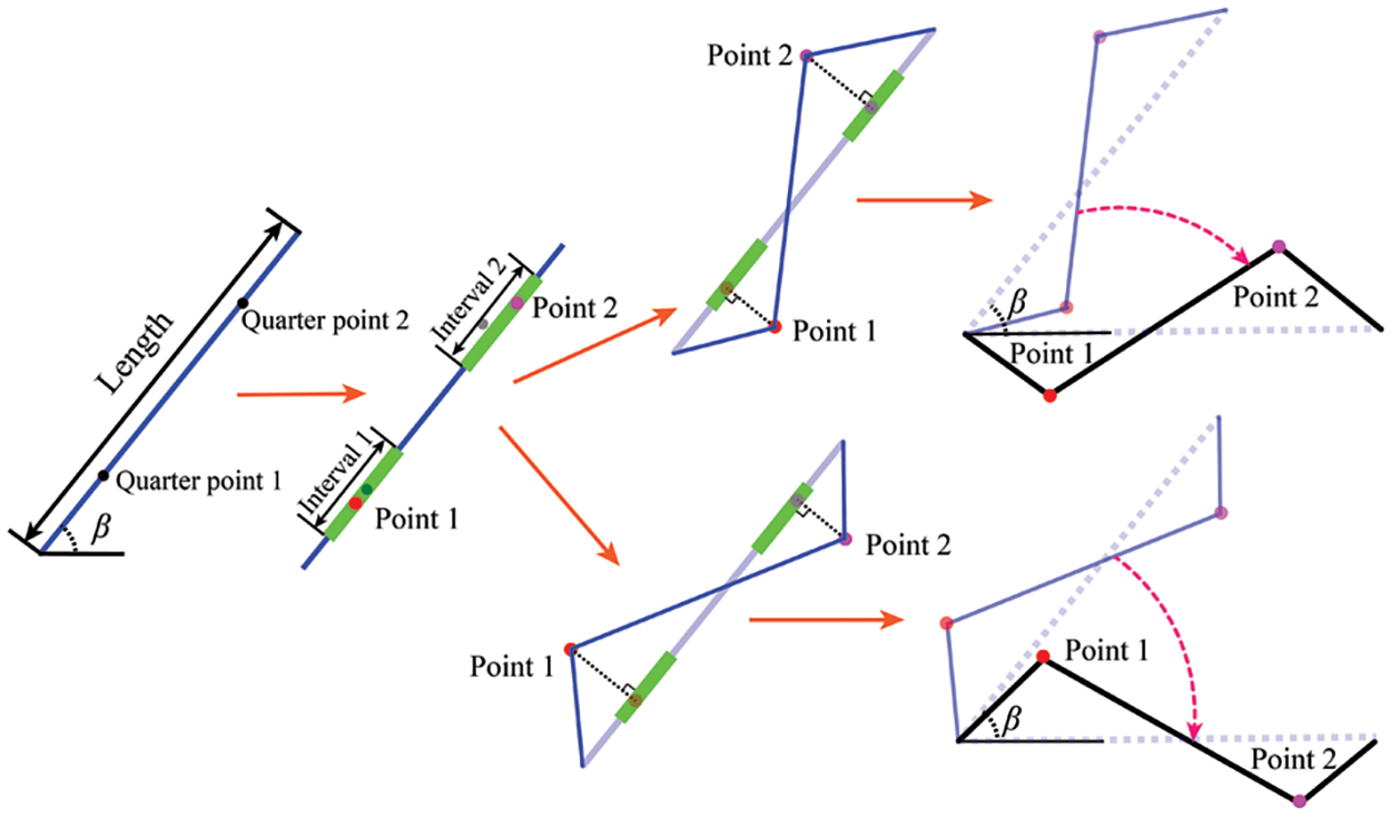
Figure 3: Polyline generation and orientation rotation
(1) Based on the stochastic distribution of discrete fractures, generate a single planar joint with a random orientation. At two quadrant points of the line segment, set two intervals with a size of 20% of the length of the line segment and then randomly select a point within each interval.
(2) Move one point in the direction perpendicular to the line segment on the randomly selected side, and the other point follows the opposite direction. The distance that points moved is specified at 0.05–0.1 of the length of the planar line.
(3) The moving points and the start and end points of the line segment are connected in sequence, leading to a polyline.
(4) Converting the orientation of this polyline to 0°, the rotation equation is as follows:
where (
2.2.2 Fractal Interpolation System
IFS is a data interpolation method based on the principle of self-similarity, which iteratively refines the local structure to produce continuous smooth curves or surfaces [28]. The points of the polyline are
where
As seen from Eq. (5), if the curve is a straight line with only the start and end points, so
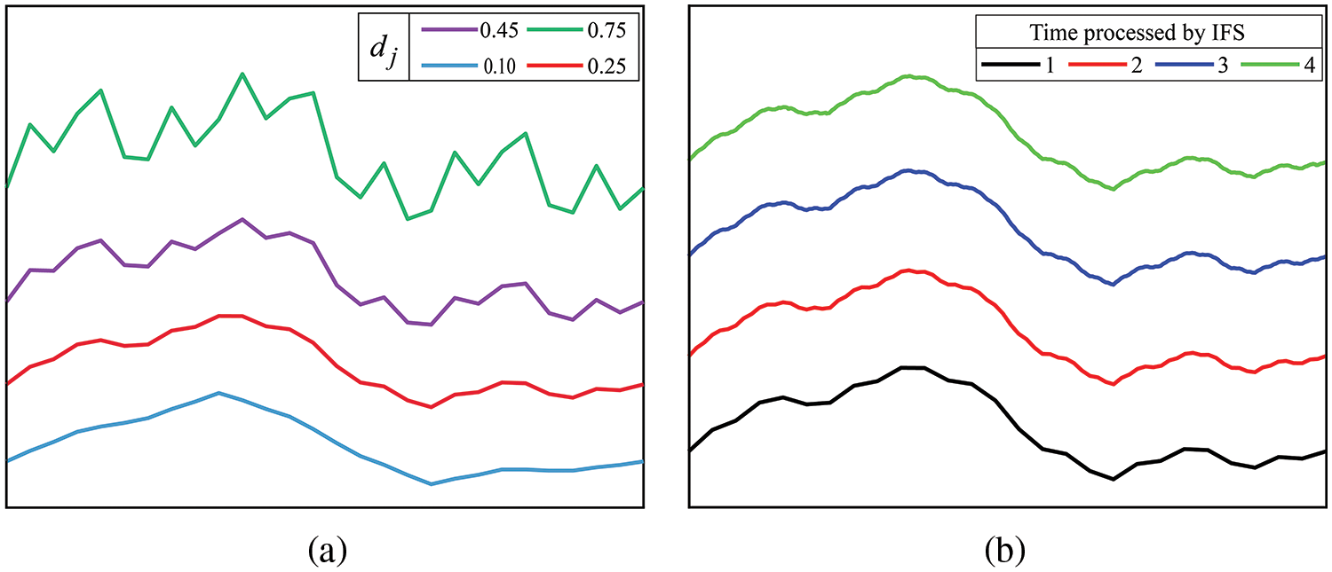
Figure 4: Fractal process with different
The curve after iteration can also continue to process with IFS to make it smoother. Fig. 4b shows the results of 4 times processing of the polyline in Section 2.2.2. The polyline processed once by IFS retains a certain level of curvature, whereas two or more iterations produce smoother results. However, with each further iteration, the number of points increases substantially. For instance, the polyline processed twice consists of 82 points, whereas one processed four times already contains 730 points. As shown in Fig. 4b, the smoothness of the above two fractal curves does not vary significantly, but the increased points will consume the memory and performance of the computer more. Therefore, in this paper, the fractal curves are only processed 2 times with IFS to balance the smoothness and computation time.
On the fractal curve, some points could be very close to each other, which will lead to numerous distorted mesh elements in the subsequent modeling process and affect the simulation results consequently. To address this, the Douglas-Peucker algorithm [30] can be applied to simplify the curve, which approach is mainly used to reduce the size of graphical and image data while preserving its fundamental shape. Its principle is to keep generating polylines to reproduce the original curve as much as possible until the distance from the point on the original curve to the polyline is less than a set threshold. The specific processes are as follows:
(1) Initial fractal curve points are entered into the algorithm, as depicted in Fig. 5a.
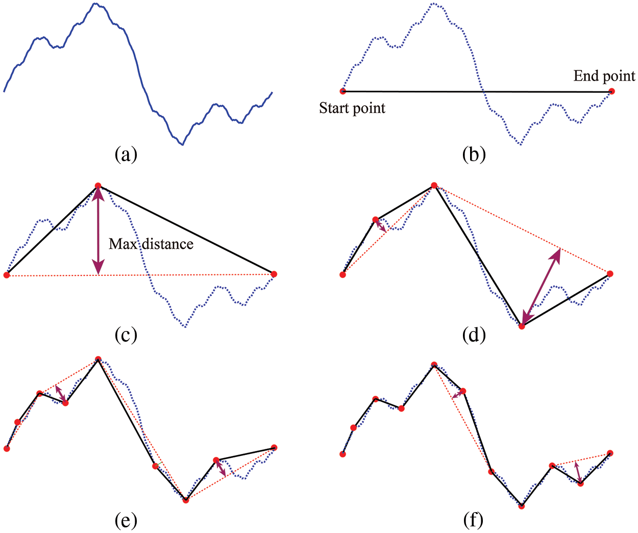
Figure 5: Process of Fractal curves smoothing: (a) initial curve; (b) select start and end point; (c) first polyline segment; (d) and (e) second and third polyline segment. (f) the final curve
(2) The simplification parameter, the maximum allowable error value (T), is specified. Select the start and end points of the fractal curve as the start and end points of the simplified planar line, as shown in Fig. 5b.
(3) The point furthest from the planar line between these two points is then selected as the inflection point, and the curve is divided into two parts, as illustrated in Fig. 5c.
(4) This process is recursively applied to these two parts until the distance of all remaining points on the fractal curve to the corresponding straight line is less than T, as demonstrated in Figs. 5d–5f.
Through this process, relatively simplified curves can be obtained, making them more suitable for modeling. By testing multiple fractal curves, setting the value of T to 0.1% of the length of the fractal curve can reduce the number of points almost 60% without changing its basic shape.
2.2.4 Numerical Modeling of Non-Prsisting Rough Open Joints
After the curves that have been simplified by the Douglas-Poker algorithm, the formation of rough open joints through them still follows the next steps.
(1) Each individual point on the rough curve is independently displaced by the same distance in two directions that are perpendicular to the line connecting the start and end points, excluding the start and end points themselves. The mean displacement distance for all points is represented by
(2) All the points on the rough curve, except for the start and end points, are deleted, and the remaining ones are connected to form a closed loop. At this moment, the open joint has been formed.
(3) Its initial orientation
where (
(4) Finally, the outer part of the open joints is meshed while preserving its geometry, and the whole process is shown in Fig. 6.
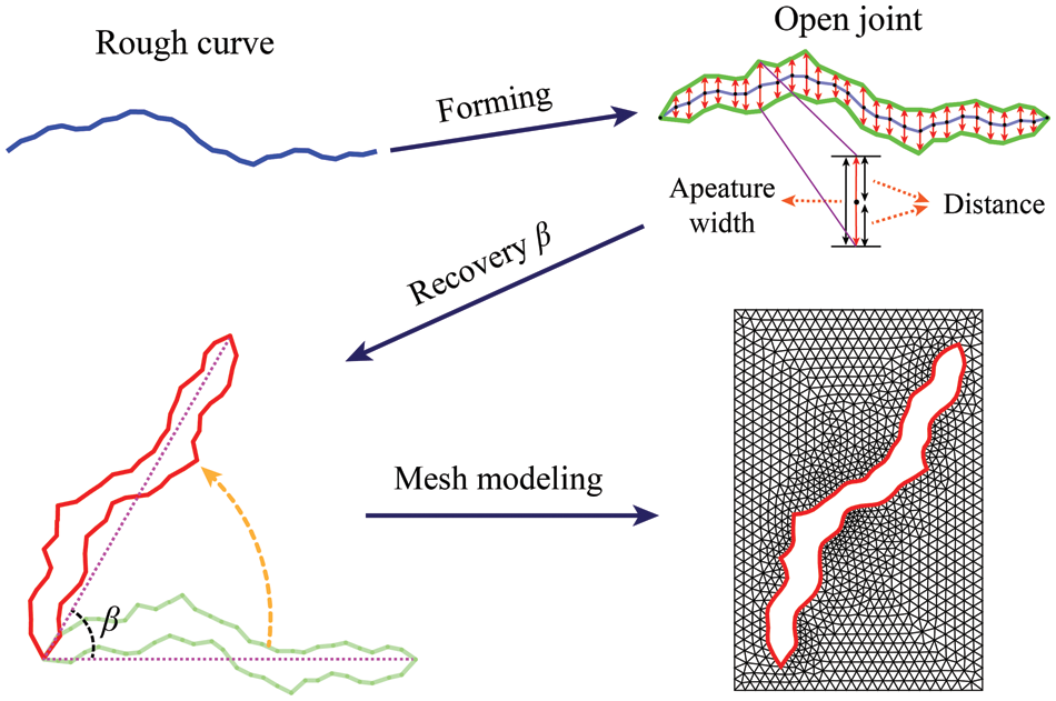
Figure 6: Process of non-persisting rough open joints modeling
2.3 Rigid Block Discrete Element Method
In recent years, DEM has been widely applied by scholars to simulate the failure process of rock mass with joints. In terms of crack initiation and propagation, the numerical results by PFC2D are in good agreement with the experimental results, and this software has been widely accepted [23–25]. Whereas, in traditional 2D DEM simulations, the ball is often selected as the basic discrete element, leading to numerous micro-voids between them, which is inconsistent with reality, as shown in Fig. 7a. Compared to the former, RB-DEM has significant advantages. In this method, each rblock is created from the finite element mesh without micro-voids. Additionally, as displayed in Fig. 7b, by specifying the shape and edge length interval of mesh elements, regular rblocks can be obtained, which eliminates the influence of complex shapes of rblocks on numerical simulations.
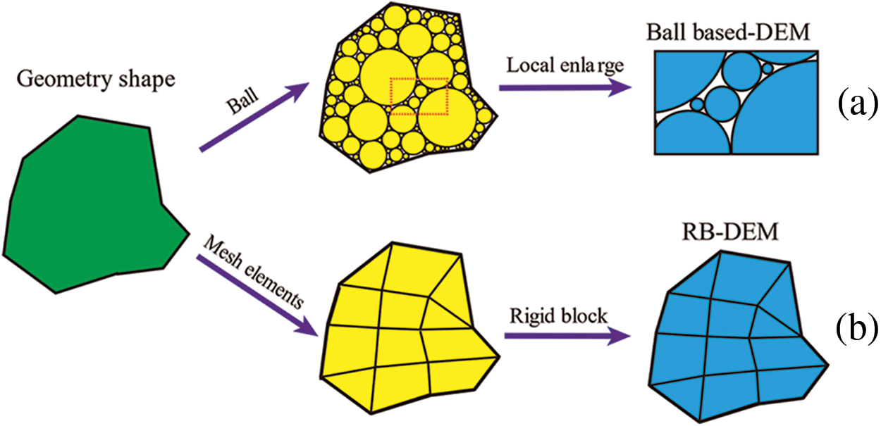
Figure 7: Two types of discrete elements: (a) ball; (b) rblock
In DEM, where discrete elements touch each other, contacts will be generated that can transfer forces and moments between them. For the open joint in the ball element model, balls are all circular and cannot clearly describe the boundary between open joints and the rock mass. For instance, as shown in Fig. 8a, it is a ball-composed model containing 9 planar open joints. The width distribution of open joints is greatly affected by the geometric defect of balls, which cannot be kept consistent. This also affects the distribution of contacts around open joints. When the model contains rough open joints with smaller widths, defects become even more pronounced. In this work, contacts also generate in the place where rblocks touch with each other. As there are no rblocks in the interior of open joints, contacts cannot appear, as illustrated in Fig. 8b. Compared with the ball, rblocks can clearly describe the boundary of joints and the rock mass. So, no matter how complex the shape of open joints is, these contacts are not affected, which is the significant advantage of rblocks. Considering the intricate and little size of meshes surrounding open joints, this work selects a mesh size range of 0.5 to 5 mm. This ensures that the fractures remain minimally influenced, while also avoiding excessive mesh that could hinder computational efficiency.
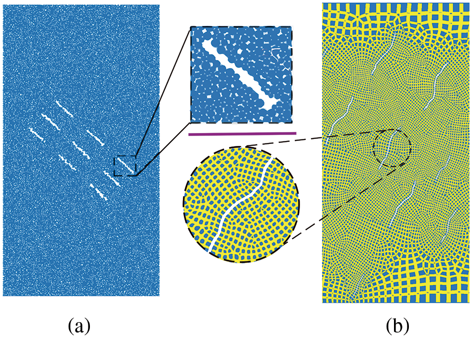
Figure 8: Rock masses with different joint types: (a) planar open joints; (b) rough open joints
2.4 Framework of Numerical Modeling and Simulation
The general process of numerical modeling and simulation of non-persisting rough open joints can be simplified into three main parts:
(1) Rough curves can be generated by using a combination of DFN stochastic distribution and the enhanced IFS method that can handle planar lines and polylines of any orientation. The Douglas-Peucker algorithm is then applied to simplify them while preserving the basic shape. Next, open joints are generated and a finite element mesh model is constructed using modeling software. Finally, the finite element model with geometric features of these joints is converted to a discrete element model based on the RB-DEM technique.
(2) Select the appropriate contact model as well as the corresponding non-relevant micromechanical parameters, and employs the Pairwise algorithm [31] to get these parameter values based on the stress-strain curve from the experimental data.
(3) Analyze the impact of orientation, aperture, and number variation of non-persisting joints on the mechanical behavior of rock mass. Based on these discussions, some conclusions and inferences, are given, and the defects that exist in this work are also analyzed.
All the specific implementation steps are shown in Fig. 9.
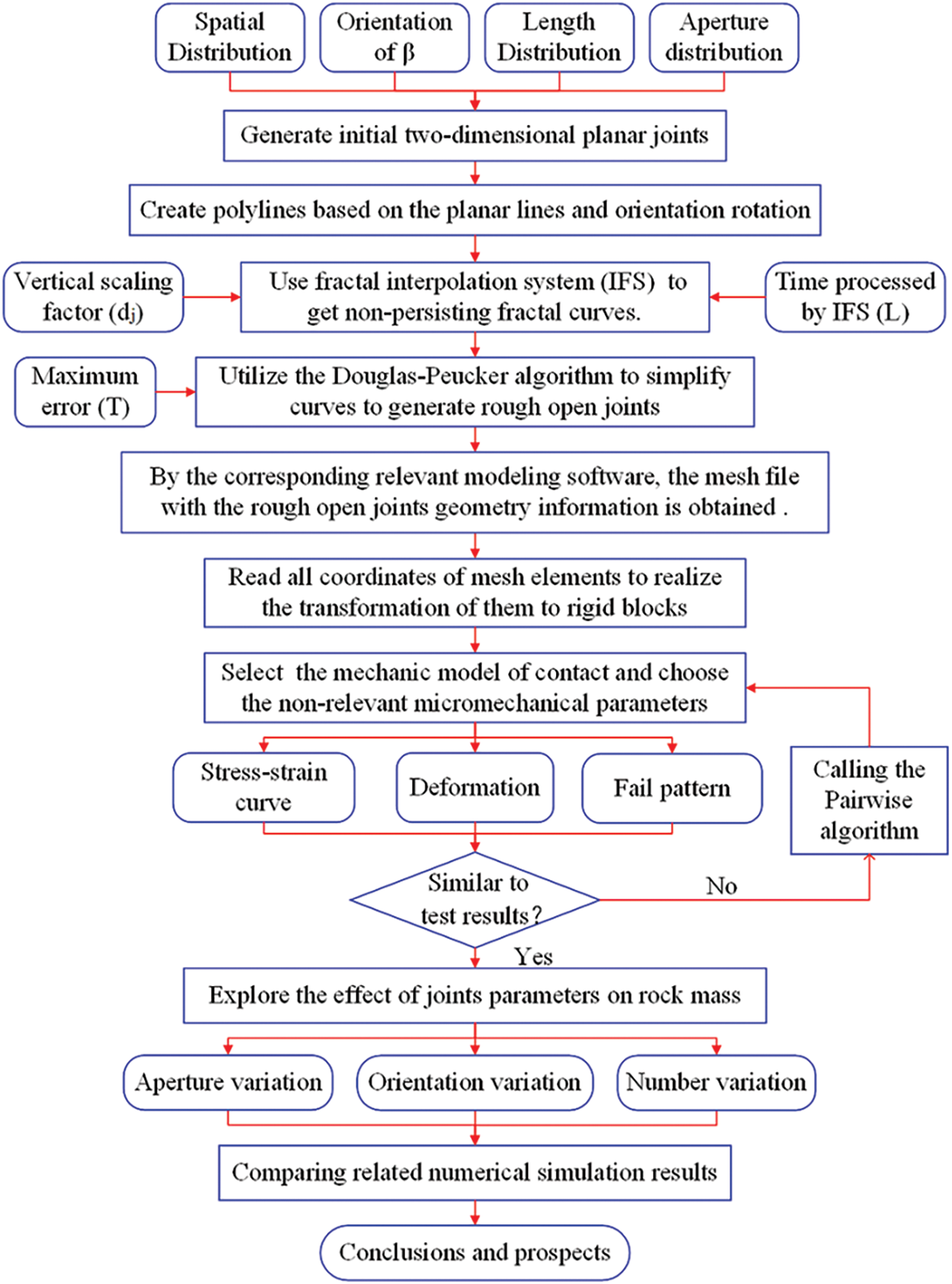
Figure 9: Flow chart for numerical modeling and simulation of non-persisting rough joints
3.1 Selection of the Contact Model
The commonly used contact models for simulating rock-like materials are the linear parallel bond (PB) contact model [39] and the flat-joint contact (FJ) model [40,41]. When using the discrete element as a ball, the PB model establishes contact at the overlapping region of balls. In contrast, the FJ model can create interlocked contacts between them, which is better suited for accurately simulating the microstructure of angular, interlocked grains resembling marble. However, the discrete elements utilized are rblocks in this study, each associated with a transformed mesh. The mesh itself possesses a prismatic shape, either quadrilateral or triangular, reducing the need to create contact with a locking foot to simulate rock-like materials. Additionally, the PB model has demonstrated its applicability in RB-DEM. For instance, Meng et al. employed the PB model to replicate the damage behavior of concrete [29], while Ding et al. utilized it to investigate the mechanical characteristics of high-volume bimrocks [42]. Therefore, the PB model is chosen to simulate the mechanical behavior of rock masses containing non-persisting rough open joints.
The PB model consists of two contact interfaces: an unbonded interface and a bonded interface. The two interfaces are shown in Fig. 10 with their respective parameters. Effective modulus of the unbonded interface and the bonded interface are represented by
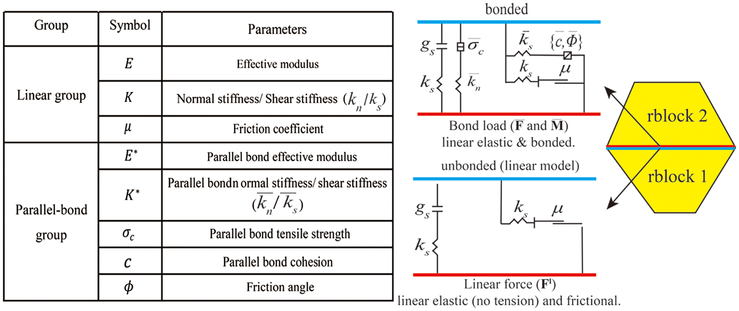
Figure 10: Two contact interfaces of the linear parallel bond model
The calibration principle adopted in this study involves determining the values of
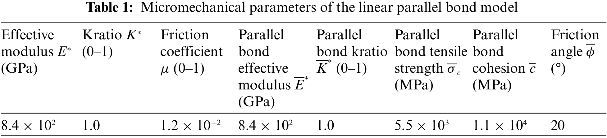
To ensure the correctness of parameters, the stress-strain curve of the rock mass specimen including 9 open joints with the orientation of 90° [44] are used as the standard for calibration. Then obtained these parameter values are also adopted for the specimen with open joints of 30° to examine the difference between the experimental and simulated data. The geometric information of the two samples is shown in Fig. 11a. The stress-strain curves from Fig. 11b demonstrate that when the uniaxial compressive strength (UCS) and the corresponding strain (Strain of UCS) are the same for both rock samples, the corresponding values for the sample with 30° joints (in Fig. 11c) are 10.78 MPa and 0.171%, and 9.98 MPa and 0.175%, respectively. The variation of UCS is 7.42% and the strain of UCS is 2.33%, which confirms the accuracy of the calibrated parameters. Table 1 displays the resulting parameter values.
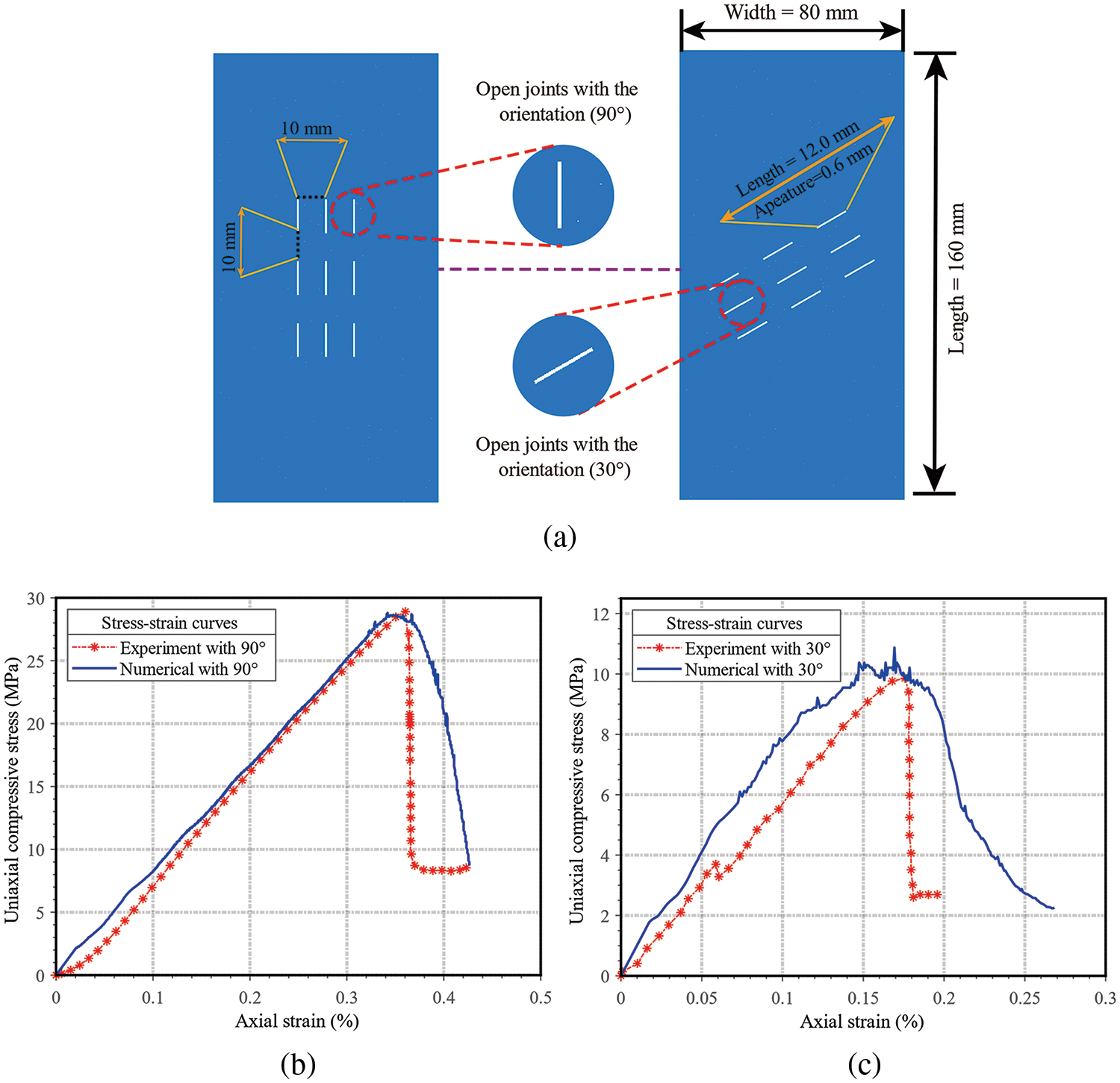
Figure 11: The geometry and stress-strain curves of two rock mass specimens: (a) the geometric information of rock mass specimens and joints; (b) stress-strain curves of the specimen of 90° joints; (c) stress-strain curves of the specimen of 30° joints
3.3 Stress-Strain Curve and Crack Evolution under Uniaxial Compression
To analyze the effect of open joints on crack development under uniaxial compression, the model with an equal open joint number are created, following the same specifications as the above experiment. The spatial location obeys relative random distribution. Set
The stress-strain curve is a significant tool to study the mechanical properties of geological materials, from which the crack initiation stress (
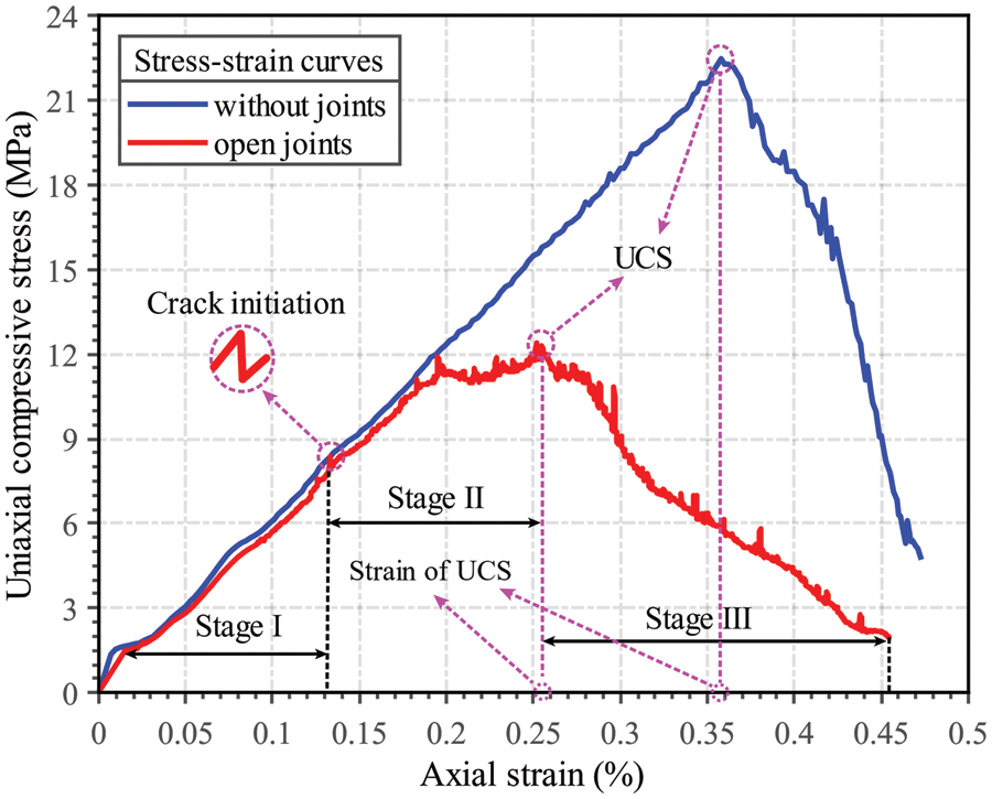
Figure 12: Stress-strain curves of two rock mass specimens
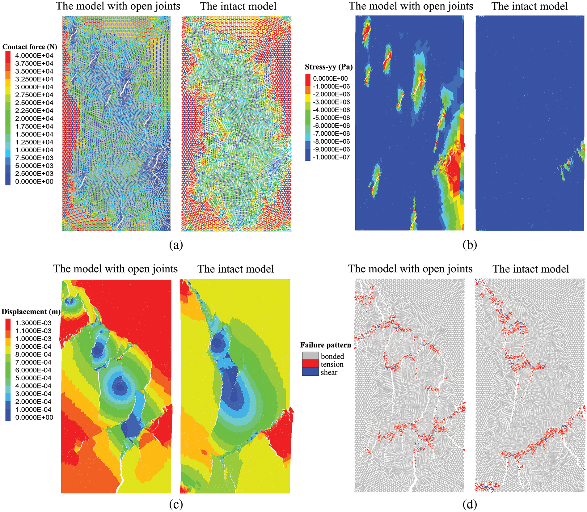
Figure 13: Comparison of rock mass specimens: (a) contact force distribution; (b) stress-yy distribution; (c) the model displacement; (d) failure pattern of contacts
During Stage III, the cracks within the jointed model continue to expand until they coalesce. At a strain of 0.45%, Fig. 13c indicates that new cracks coalesce off all joints with a higher number. Furthermore, cracks are more distorted in the model with open joints, indicating that the joint has a significant effect on crack development. The contact failure pattern shown in Fig. 13d reveals that a large number of damaged contacts are concentrated at both ends of cracks and are dominated by tensile failure. This is consistent with the effect of planar open joints on rock mass in uniaxial loading.
4.1 Effect of Different Orientations
Previous experiments and simulations proved that the orientation of joints has a great influence on the strength and fracture development of rock-like or brittle materials [45]. However, only a few joints are often generated experimentally, and the real geometry of the joints cannot be reproduced in numerical simulations. Based on the technique in this paper, rock mass models including 27 rough open joints are generated in this work, respectively, with average orientations ranging from 0° to 90° at 15° intervals and a standard deviation of 2°. The statistical distribution pattern of the joints is maintained as in Section 3.2, with the exception that
Fig. 14a presents stress-strain curves for models containing 27 open joints with different average orientations, demonstrating that all have three phases, but exhibit significant differences. Firstly, as the orientation increases,
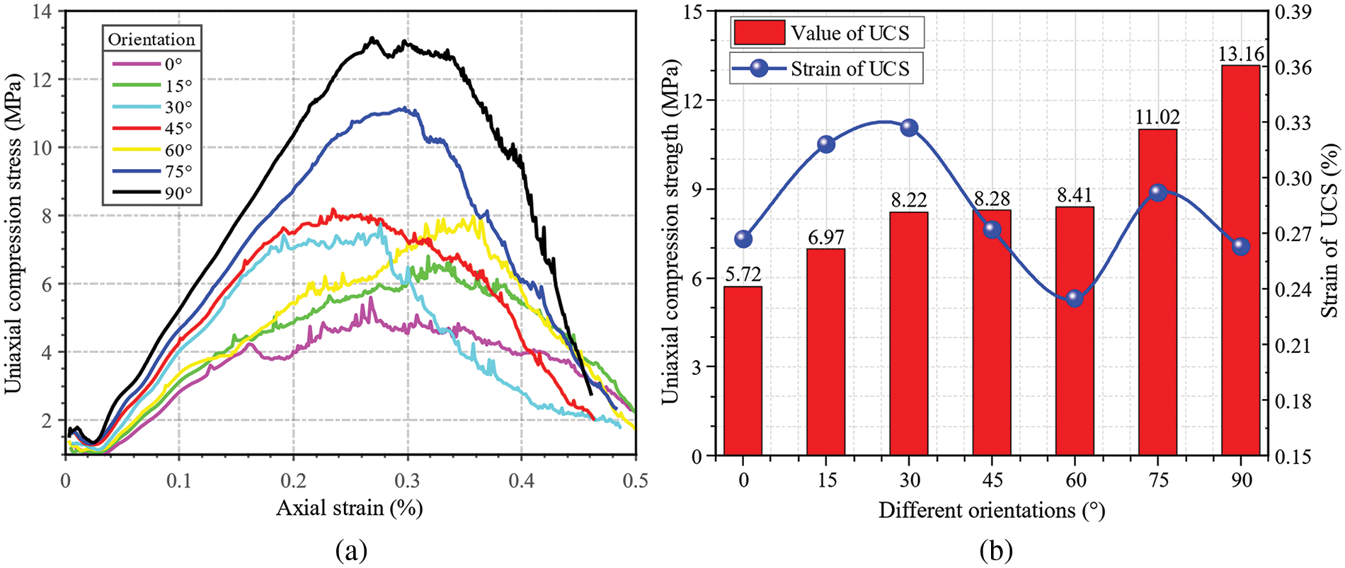
Figure 14: Effect of joint orientations on models: (a) stress-strain curves; (b) variation of UCS as well as the corresponding strain
Fig. 15 shows the displacement distribution after the damage of these models. The crack distribution varies more between models with open joints at different orientations, which means that the orientation of joints can have a significant impact on the development of new cracks. Mostly new cracks are perpendicular to the loading direction. When the orientation is lower, cracks are relatively more tortuous, which also causes the corresponding stress-strain curves to be relatively more prone to fluctuations. Additionally, excluding the model of
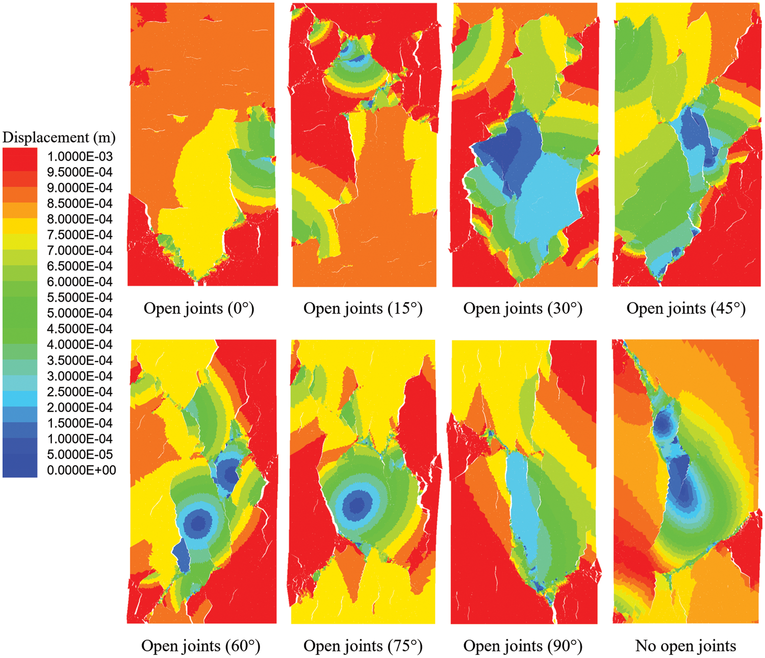
Figure 15: Displacement of models containing joints with different orientations and the intact model
To investigate the impact of aperture width on rock mass strength, simulations are conducted on specimens with 27 joints with average orientations of 0°, 30°, 60°, and 90°, and a standard deviation of 2°, using uniaxial loading. The study tests five ratios of mean aperture size to the length of each joint at 2%, 4%, 6%, and 8% denoted by
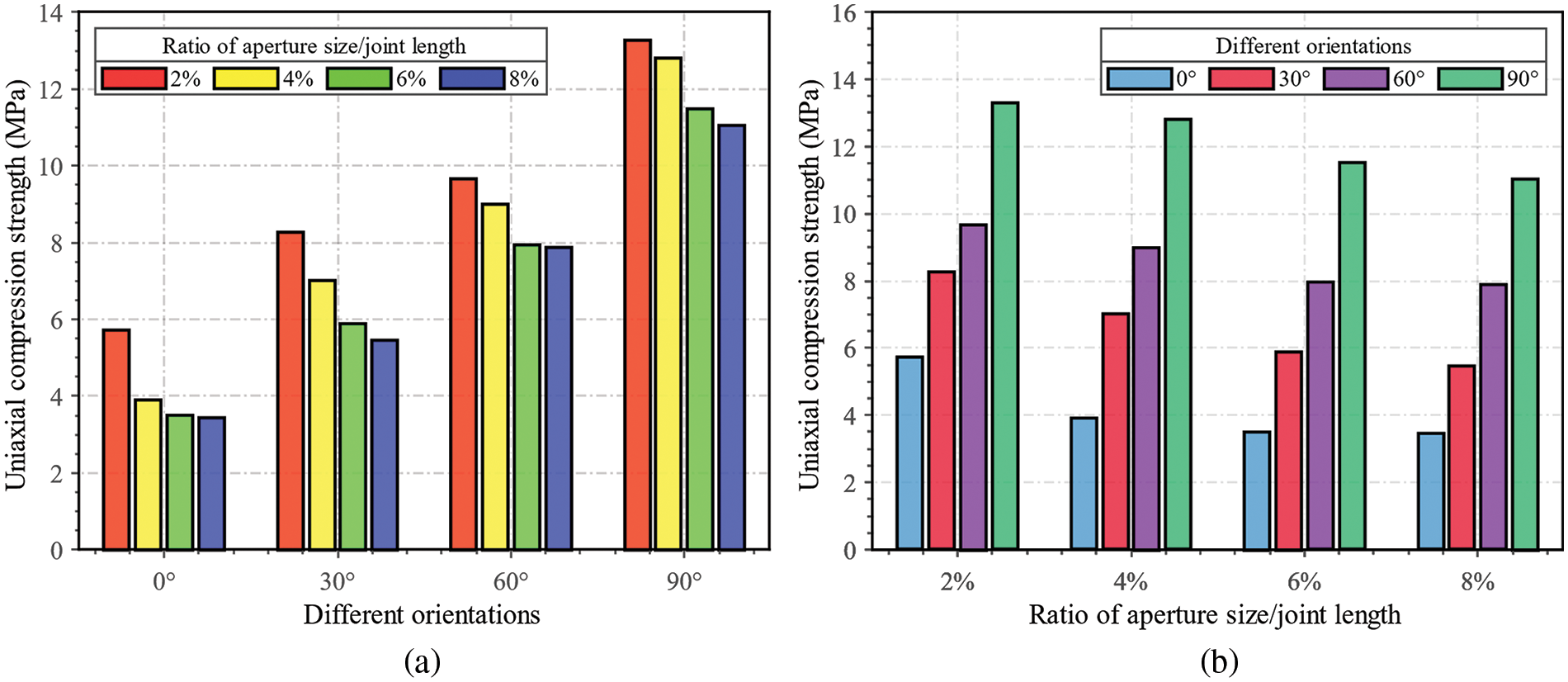
Figure 16: The UCS values of models containing joints with different aperture widths and orientations: (a) different orientations; (b) different ratios of aperture width/joint length
Fig. 17 shows the stress-yy distribution for all models when the compressive stress reaches UCS, ranging from 0 to −10 MPa, where −10 MPa indicates compressive stress, and the red region indicates the compressive stress that has either reached or exceeded 10 MPa. The model with joints having an aperture size to joint size ratio of 2% and an orientation of 90° gets the highest UCS due to the largest red area. At an orientation of 0°, the red region experiences a drastic decline and is virtually absent throughout the model as the aperture ratio increases to 8%, which is the primary reason for its largest drop in UCS. In contrast, the red area at other orientations decreases, but the trend slows down significantly as the joint orientation increases, explaining why the drop in UCS gradually decreases as joint orientation increases. Additionally, at the same aperture ratio, the red region enlarges with the increase of orientation, mainly when the aperture ratio is 8%. It can be predicted that the UCS is more sensitive to joint orientation than its aperture ratio.
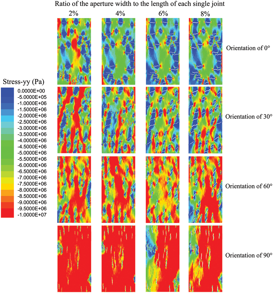
Figure 17: Stress-yy of open joints with different aperture widths and orientations
4.3 Effect of the Joint Number
Numerous prior experiments have analyzed the impact of joint density on the mechanical characteristics of rocks [16,36]. To examine its effect, samples containing various numbers of joints were created, including 9, 18, 27, 36, and 45. The length of joints is established at 12 mm (
where
The UCS of the corresponding models is shown in Fig. 18, which exhibits a significant decrease with increasing joint density across all three angles. Specifically, the 15° model experiences a decrease in strength from 9.32 to 5.15 MPa, the 45° model from 10.51 to 5.95 MPa, and the 75° model from 20.01 to 10.73 MPa, resulting in an average reduction rate of 44.98%. The distribution of contact force is taken for all models when the compressive stress reaches UCS, as shown in Fig. 19. The force interval is set between 0 to 15 kN. Where the red contact represents its force has already reached or exceeded 15 kN. There is no contact generation at these joints, resulting in the disruption of force transmission and limiting the capacity of the surrounding contact load-bearing capacity. Especially when the joint density reaches 4.22% (the joint number is 45), a considerable amount of red contact disappears. At this moment, it is easier to observe red contacts at the ends of joints, which is why new cracks tend to initiate from these locations. The joint density has a significant weakening effect on the mechanical properties of the rock masses, which is consistent with the conclusions obtained by previous scholars.
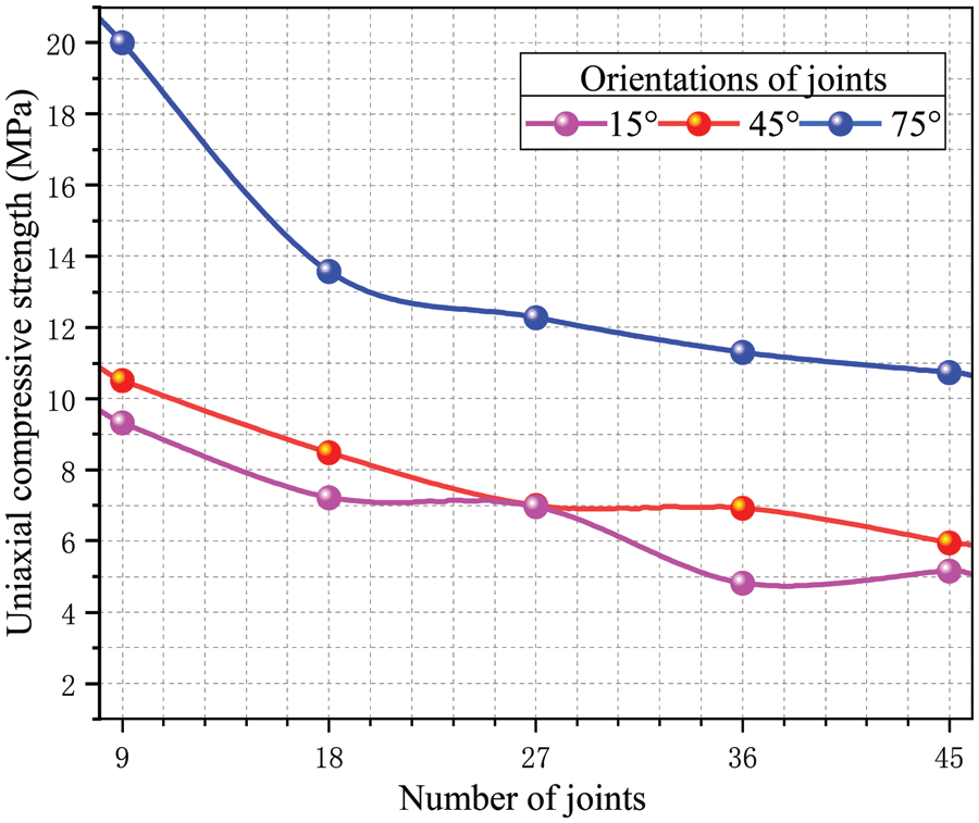
Figure 18: UCS of models containing different joint numbers
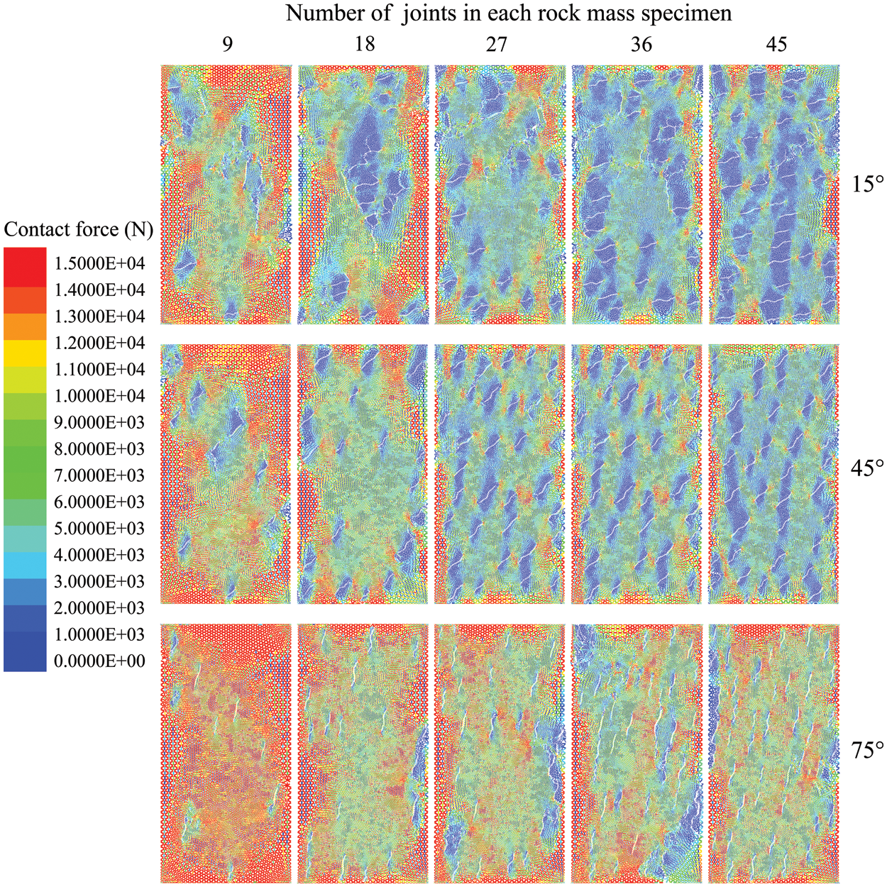
Figure 19: Contact force distribution of models with different joint numbers
In this study, based on the IFS-enhanced method and the RB-DEM modeling technique, the discrete element model containing non-persisting rough open joints with different orientations and aperture widths can be generated. In addition, the influence of the orientation, aperture width as well as joint number are also discussed in a series of uniaxial compression simulations. The main conclusions can be summarized below:
(1) The orientation of open joints has a significant impact on the models. Even with the same number of open joints, variations in orientation can result in more than a twofold change in the UCS. This effect is particularly pronounced when the orientation angle is small, leading to a more pronounced weakening effect.
(2) The aperture width of joints can alter the stress distribution and weaken the load-bearing capacity of the rock mass. However, the rate of decrease in UCS slows down as the ratio of aperture size to joint length increases. Additionally, increasing the aperture width does not change the trend of UCS with respect to joint orientation.
(3) A high number of joints can impede force transmission within the model and limit the load-carrying capacity of contacts surrounding the joints. This significantly affects the mechanical properties of rock masses. Therefore, during engineering construction activities, timely support measures are crucial to prevent the excessive occurrence of open joints in the surrounding rock.
However, this study also has certain limitations. The use of 2D joints disregards the impact of longitudinal stress, resulting in an incomplete representation of the three-dimensional characteristics of natural geological formations. Additionally, the 2D rock models might underestimate the extent of deformation and damage, particularly in scenarios involving complex loading conditions for rock masses. As a result, there is a critical need to advance the development of more realistic 3D non-persisting rough open joints to address these limitations effectively.
Acknowledgement: The authors would like to express their appreciation to the editor and reviewers for their valuable suggestions which greatly improved the presentation of this paper.
Funding Statement: This investigation is financially supported by the National Key R&D Program of China (2018YFC0407004), the Fundamental Research Funds for the Central Universities (Nos. B200201059, 2021FZZX001-14), the National Natural Science Foundation of China (Grant No. 51709089) and 111 Project.
Author Contributions: The authors confirm contribution to the paper as follows: study conception and design: Hangtian Song, Qingxiang Meng; data collection: Hangtian Song, Xudong Chen; analysis and interpretation of results: Hangtian Song, Chun Zhu, Qian Yin; draft manuscript preparation: Hangtian Song, Wei Wang. All authors reviewed the results and approved the final version of the manuscript.
Availability of Data and Materials: The data that support the findings of this study are available on request from the corresponding author, upon reasonable request.
Conflicts of Interest: The authors declare that they have no conflicts of interest to report regarding the present study.
References
1. Bobet, A. (2000). The initiation of secondary cracks in compression. Engineering Fracture Mechanics, 66(2), 187–219. [Google Scholar]
2. Chen, M., Zang, C. W, Ding, Z. W, Zhou, G. L, Jiang, B. Y. et al. (2022). Effects of confining pressure on deformation failure behavior of jointed rock. Journal of Central South University, 29(4), 1305–1319 (In Chinese). [Google Scholar]
3. Li, L., Wu, W., El Naggar, M. H., Mei, G., Liang, R. (2019). Characterization of a jointed rock mass based on fractal geometry theory. Bulletin of Engineering Geology and the Environment, 78(8), 6101–6110. [Google Scholar]
4. He, M., Wang, H., Ma, C., Zhang, Z., Li, N. (2023). Evaluating the anisotropy of drilling mechanical characteristics of rock in the process of digital drilling. Rock Mechanics and Rock Engineering, 56(5), 3659–3677. [Google Scholar]
5. Wang, H., He, M., Zhang, Z., Zhu, J. (2022). Determination of the constant mi in the Hoek-Brown criterion of rock based on drilling parameters. International Journal of Mining Science and Technology, 32(4), 747–759. [Google Scholar]
6. Afifipour, M., Moarefvand, P. (2014). Mechanical behavior of bimrocks having high rock block proportion. International Journal of Rock Mechanics and Mining Sciences, 65, 40–48. [Google Scholar]
7. Cao, P., Liu, T., Pu, C., Lin, H. (2015). Crack propagation and coalescence of brittle rock-like specimens with pre-existing cracks in compression. Engineering Geology, 187, 113–121. [Google Scholar]
8. Chen, X., Liao, Z., Peng, X. (2012). Deformability characteristics of jointed rock masses under uniaxial compression. International Journal of Mining Science and Technology, 22(2), 213–221. [Google Scholar]
9. Lee, H., Jeon, S. (2011). An experimental and numerical study of fracture coalescence in pre-cracked specimens under uniaxial compression. International Journal of Solids and Structures, 48(6), 979–999. [Google Scholar]
10. Yang, S. (2013). Study of strength failure and crack coalescence behavior of sandstone containing three pre-existing fissures. Rock Soil Mechanics, 34(1), 31–39. [Google Scholar]
11. Lajtai, E., Carter, B., Duncan, E. (1994). En echelon crack-arrays in potash salt rock. Rock Mechanics and Rock Engineering, 27, 89–111. [Google Scholar]
12. Esterhuizen, G., Dolinar, D., Ellenberger, J. (2011). Pillar strength in underground stone mines in the United States. International Journal of Rock Mechanics and Mining Sciences, 48(1), 42–50. [Google Scholar]
13. Sagong, M., Bobet, A. (2002). Coalescence of multiple flaws in a rock-model material in uniaxial compression. International Journal of Rock Mechanics and Mining Sciences, 39(2), 229–241. [Google Scholar]
14. Park, C., Bobet, A. (2010). Crack initiation, propagation and coalescence from frictional flaws in uniaxial compression. Engineering Fracture Mechanics, 77(14), 2727–2748. [Google Scholar]
15. Vaziri, M. R., Tavakoli, H., Bahaaddini, M. (2022). Statistical analysis on the mechanical behaviour of non-persistent jointed rock masses using combined DEM and DFN. Bulletin of Engineering Geology and the Environment, 81(5), 177.1–177.24. [Google Scholar]
16. Bahaaddini, M., Sharrock, G., Hebblewhite, B. (2013). Numerical investigation of the effect of joint geometrical parameters on the mechanical properties of a non-persistent jointed rock mass under uniaxial compression. Computers and Geotechnics, 49, 206–225. [Google Scholar]
17. Ghazvinian, A., Sarfarazi, V., Schubert, W., Blumel, M. (2012). A study of the failure mechanism of planar non-persistent open joints using PFC2D. Rock Mechanics and Rock Engineering, 45, 677–693. [Google Scholar]
18. Chheng, C., Likitlersuang, S. (2018). Underground excavation behaviour in Bangkok using three-dimensional finite element method. Computers and Geotechnics, 95, 68–81. [Google Scholar]
19. Guo, S., Qi, S., Zou, Y., Zheng, B. (2017). Numerical studies on the failure process of heterogeneous brittle rocks or rock-like materials under uniaxial compression. Materials, 10(4), 378. [Google Scholar] [PubMed]
20. Hatzor, Y. H., Arzi, A., Zaslavsky, Y., Shapira, A. (2004). Dynamic stability analysis of jointed rock slopes using the DDA method: King Herod’s Palace, Masada, Israel. International Journal of Rock Mechanics and Mining Sciences, 41(5), 813–832. [Google Scholar]
21. Lu, Y., Tan, Y., Li, X. (2018). Stability analyses on slopes of clay-rock mixtures using discrete element method. Engineering Geology, 244, 116–124. [Google Scholar]
22. Donzé, F. V., Richefeu, V., Magnier, S. A. (2009). Advances in discrete element method applied to soil, rock and concrete mechanics. Electronic Journal of Geotechnical Engineering, 8(1), 44. [Google Scholar]
23. Zhang, X. P., Wong, L. N. Y. (2012). Cracking processes in rock-like material containing a single flaw under uniaxial compression: A numerical study based on parallel bonded-particle model approach. Rock Mechanics and Rock Engineering, 45, 711–737. [Google Scholar]
24. Cao, R. H, Cao, P., Lin, H., Pu, C. Z, Ou, K. (2016). Mechanical behavior of brittle rock-like specimens with pre-existing fissures under uniaxial loading: Experimental studies and particle mechanics approach. Rock Mechanics and Rock Engineering, 49, 763–783. [Google Scholar]
25. Sarfarazi, V., Ghazvinian, A., Schubert, W., Blumel, M., Nejati, H. (2014). Numerical simulation of the process of fracture of echelon rock joints. Rock Mechanics and Rock Engineering, 47, 1355–1371. [Google Scholar]
26. Li, K. (2004). Characterization of rock heterogeneity using fractal geometry. SPE International Thermal Operations and Heavy Oil Symposium and Western Regional Meeting, OnePetro. [Google Scholar]
27. Meng, Q., Xue, H., Zhuang, X., Zhang, Q., Zhu, C. et al. (2023). An IFS-based fractal discrete fracture network for hydraulic fracture behavior of rock mass. Engineering Geology, 324, 107247. [Google Scholar]
28. Yang, L. L., Xu, W. Y., Meng, Q. X., Wang, R. B. (2017). Investigation on jointed rock strength based on fractal theory. Journal of Central South University, 24(7), 1619–1626. [Google Scholar]
29. Meng, Q., Xue, H., Song, H., Zhuang, X., Rabczuk, T. (2023). Rigid-block DEM modeling of mesoscale fracture behavior of concrete with random aggregates. Journal of Engineering Mechanics, 149(2), 04022114. [Google Scholar]
30. Douglas, D. H., Peucker, T. K. (1973). Algorithms for the reduction of the number of points required to represent a digitized line or its caricature. Cartographica: The International Journal for Geographic Information and Geovisualization, 10(2), 112–122. [Google Scholar]
31. Thurstone, L. L. (1927). A law of comparative judgment. Psychological Review, 34(4), 273–286. [Google Scholar]
32. Gómez, S., Sanchidrián, J. A., Segarra, P., Bernardini, M. (2023). A Non-parametric discrete fracture network model. Rock Mechanics and Rock Engineering, 56(5), 3255–3278. [Google Scholar]
33. Yin, T., Chen, Q. (2020). Simulation-based investigation on the accuracy of discrete fracture network (DFN) representation. Computers and Geotechnics, 121, 103487. [Google Scholar]
34. Yoon, S., Hyman, J. D., Han, W. S., Kang, P. K. (2023). Effects of dead-end fractures on non-fickian transport in three-dimensional discrete fracture networks. Journal of Geophysical Research: Solid Earth, 128(7), e2023JB026648. [Google Scholar]
35. Zhu, W., Khirevich, S., Patzek, T. W. (2022). HatchFrac: A fast open-source DFN modeling software. Computers and Geotechnics, 150, 104917. [Google Scholar]
36. Hu, J. X., K, K., Liu, J., Xie, Z. Y., Chen, M. et al. (2022). Particle flow code analysis of the effect of discrete fracture network on rock mechanical properties and acoustic emission characteristics. Rock and Soil Mechanics, 43(S1) (In Chinese). [Google Scholar]
37. Iwano, M., Einstein, H. H. (1995). Laboratory experiments on geometric and hydromechanical characteristics of three different fractures in granodiorite. 8th ISRM Congress, OnePetro. [Google Scholar]
38. Mandelbrot, B. (1967). How long is the coast of Britain? Statistical self-similarity and fractional dimension. Science, 156(3775), 636–638. [Google Scholar] [PubMed]
39. Potyondy, D. O., Cundall, P. A. (2004). A bonded-particle model for rock. International Journal of Rock Mechanics and Mining Sciences, 41(8), 1329–1364. [Google Scholar]
40. Bahaaddini, M., Sheikhpourkhani, A. M., Mansouri, H. (2021). Flat-joint model to reproduce the mechanical behaviour of intact rocks. European Journal of Environmental and Civil Engineering, 25(8), 1427–1448. [Google Scholar]
41. Gutiérrez-Ch, J. G., Senent, S., Melentijevic, S., Jimenez, R. (2018). Distinct element method simulations of rock-concrete interfaces under different boundary conditions. Engineering Geology, 240, 123–139. [Google Scholar]
42. Ding, Y., Zhang, Q., Zhao, S., Chu, W., Meng, Q. (2023). An improved DEM-based mesoscale modeling of bimrocks with high-volume fraction. Computers and Geotechnics, 157, 105351. [Google Scholar]
43. Sinha, S., Walton, G. (2020). A study on bonded block model (BBM) complexity for simulation of laboratory-scale stress-strain behavior in granitic rocks. Computers and Geotechnics, 118, 103363. [Google Scholar]
44. Chen, M., Yang, S., Pathegama Gamage, R., Yang, W., Yin, P. et al. (2018). Fracture processes of rock-like specimens containing nonpersistent fissures under uniaxial compression. Energies, 12(1), 79. [Google Scholar]
45. He, M., Zhao, J., Deng, B., Zhang, Z. (2022). Effect of layered joints on rockburst in deep tunnels. International Journal of Coal Science & Technology, 9(1), 21. [Google Scholar]
Cite This Article
 Copyright © 2024 The Author(s). Published by Tech Science Press.
This work is licensed under a Creative Commons Attribution 4.0 International License , which permits unrestricted use, distribution, and reproduction in any medium, provided the original work is properly cited.
 Downloads
 Citation Tools