Multi-Level Parallel Network for Brain Tumor Segmentation

1  Introduction

The brain is one of the most important organs of human beings. No matter whether the brain tumor is benign or malignant, once it constricts any part of the brain, it will cause different damage to the human body, threatening human health and life. In China, according to the latest national cancer statistics released by the National Cancer Center, the new incidence rate of brain tumors in 2016 increased by 2.8% compared with 2015, reaching 109,000 people, and the death rate of brain tumors increased by 4.5%, reaching 59,000 people [1,2]. Glioma is the most common primary brain tumor and is classified into high-grade (HGG) and low-grade glioma (LGG) [3]. HGG grows fast with high malignant and invasion, recurs quickly after surgery, and the prognosis is relatively poor. Usually, the survival time of patients is about two years after diagnosis [4]. Although LGG is not biologically benign, the prognosis of patients is relatively good, and some patients can be cured by surgery. Computed Tomography (CT) and Magnetic Resonance Imaging (MRI) are popular imaging methods. Although the spatial resolution of CT images is high, the resolution of soft tissue is low, so it cannot provide tissue biological state information. Therefore, brain CT scanning mainly determines whether intracranial space occupies lesions preliminarily. If intracranial space occupies the lesion, an MRI scan is required for further detailed examination and confirmation. MRI is superior to CT in displaying the location, size, and shape of tumors and, therefore, has gained more attention in clinical diagnosis of brain tumors. MRI scanning can obtain multimodal images using various imaging technologies. The T1-weighted (T1), post-contrast T1-weighted (T1Gd), T2-weighted (T2), and fluid-attenuated inversion recovery (FLAIR) are four common multimodal scans that provide plentiful and complementary biological information of tumor and reveal its internal structure [5]. Accurately segmenting gliomas and their internal structure is important for treatment plans, therapeutic processes, and follow-up studies. Due to the high heterogeneity of glioma in different tumor appearance shapes and a small proportion of brain tumors in MRI brain images, automatically segmenting tumors is challenging, especially in small sub-region segmentation of brain tumors.

In recent years, deep learning methods, especially convolutional neural networks (CNNs), have made remarkable achievements in brain tumor segmentation in MRI images [6–10]. InputCascadeCNN, proposed by Havaei et al. [6], extracted the local and global context of input patches using two-pathway CNNs and took first place in the BraTS 2015 competition. Pereira et al. [7] used small 3 × 3 kernels in CNN architecture and obtained an excellent performance on tumor segmentation. Dvorak et al. [8] used a CNN with 6 layers for local structure prediction for 3D tumor segmentation, achieving successful results. Urban et al. [9] adopted 3D CNN with three layers for brain tumor segmentation, and Kamnitsas et al. [10] proposed 3D CNN with 11 layers and used CRF in post-processing. Both 3D CNNs attained superior results.

In deep neural networks, the final high-level feature has a large receptive field with global context and strong semantic information representation but with low resolution and less spatial details information because of many pooling and stridden convolutions. Moreover, the low-level feature from the shallow network contains finer spatial information with high resolution but lacks strong semantic information. Low-level spatial information is important to segment the boundaries or local details accurately. Fusing high-level semantic abstracts and low-level spatial information improves image classification and segmentation accuracy [11,12]. Serial and parallel network structures are popular fusion strategies.

The Fully Convolutional Network (FCN) [11] and U-Net [12] are typical serial networks that use down-sampling to reduce the resolution and enlarge the receptive field to obtain rich features. In order to remedy the detailed information lost in the repeated pooling and stridden convolution to generate high-resolution prediction, serial networks use up-sampling to increase the resolution and facilitate skip-connection to fuse the low-level and high-level feature information. U-Net has been the popular network in medical image segmentation since it was presented, as many top MRI brain tumor segmentation methods use U-Net as the backbone network [13–16]. Myronenko [13] proposed a 3D U-Net with a variational auto-encoder (VAE) branch to regularize the shared encoder for MRI image brain segmentation and received first place in the BraTS 2018 competition. Isensee et al. [14] presented a modified 3D U-Net, which focused on data pre-processing, training, and post-processing methods and achieved outstanding brain tumor segmentation performance. Jiang et al. [15] proposed a two-stage cascaded U-Net for brain tumor segmentation from coarse to fine, where the prediction results of the first-stage network are used as the input of the second-stage network with two decoders. Jiang et al. achieved first place in BraTS 2019. Jia et al. [16], the second winner of BraTS 2020, proposed a hybrid high-resolution and non-local feature network (H2NF-Net) for brain tumor segmentation, where a single HNF-Net is an encoder-decoder structure dealing with the original scale and four cascaded multiscale fusion modules at different scales. The network maintains the high-resolution features to represent and aggregate multiscale context information. Chang et al. [17] presented a residual dual-path attention fusion U-shaped network (DPAFNet), in which dual paths expand network scale and attention merging to fuse local and global information over channels. DPAFNet achieved promising results on BraTS 2018, BraTS 2019 and BraTS 2020 datasets. Lu et al. [18] designed a 3D multiscale Ghost convolution neural network with an auxiliary MetaFormer decoding path (GMetaNet), which extracted local-global feature information using the Ghost spatial pyramid module and obtained long-range dependencies with Ghost self-attention. GMetaNet achieved desirable results with low spatial and time complexity.

In a parallel network for multiscale fusion, each branch is independent and has different weights and feature maps with no hierarchical relationship. The parallel network has advantages similar to ensemble learning, which reduces the feature maps’ errors and the network’s variance [19]. Szegedy et al. [20] proposed an Inception module to fuse multiscale output features using four parallel branches with three different-sized convolution kernels and a pooling layer, achieving excellent image classification and detection performance. SPP network [21] adopted the spatial pyramid pooling layer to use different scale max pooling for input features to extract different features, which is easier to converge and has high accuracy. ASPP network [22] employed atrous convolution with different rates to capture context information on multiscale in parallel ways [23] and fused features from four branches with different pyramid scales. The ASPP is top-ranked in the PASCAL VOC-2012 semantic image segmentation task. Lin et al. [24] claimed that up-sampling cannot recover the information lost in down-sampling processing when using CNN for image semantic segmentation, resulting in low accuracy. The authors presented RefineNet, which exploited all scale information in the down-sampling process, and different scale features are propagated in multi-path and then are fused by summation. This network performs well in image semantic segmentation. Parallel multiscale feature fusion methods have been used in MRI image brain tumor segmentation to achieve good performance. DeepMedic [10] comprises two parallel pathways, each processing input MRI images at different resolutions simultaneously to combine local and larger context information. DeepMedic obtained the top segmentation performance for brain tumor segmentation in BraTS 2015. Besides, Xu et al. [25] proposed a multiscale masked 3D U-Net that extracts multiscale information by feeding multi-resolution patches as input and using a 3D ASPP module. The authors segmented three tumor sub-regions sequentially by keeping the segmented larger region tumor as a mask for smaller region tumors and achieved appealing results for small tumor areas. Chen et al. [26] introduced a new 3D dilated multi-fiber network (DMFNet) for 3D MRI brain tumor segmentation, which employed three weighted 3D dilated convolutions to enlarge their receptive fields and capture multiscale 3D feature maps and add them together. This weighted sum algorithm helps select the most valuable information automatically from different fields of view.

Although 3D CNNs using multiscale fusion strategies through serial or parallel networks have significantly improved tumor segmentation accuracy, some challenges still need to be addressed. Firstly, repeated down-sampling operations, such as pooling or stride convolution in CNNs, lead to the loss of low-level precise spatial information and mid-level object parts information. The features from the middle layer are between the low-level and the high-level features, which are complementary to the low-level spatial information and the high-level semantic information [24]. The loss of low-level and mid-level information will affect the performance of tumor segmentation, especially in small regions. The above references about brain tumor segmentation mainly focus on the learning and fusion of high-resolution semantic and low-resolution spatial information but do not pay enough attention to the information on mid-level features. Secondly, how to solve the class imbalance and the output imbalance (between false positive and false negative samples) in the inference stage deserves more discussion and attention. Therefore, we propose a multi-level parallel network for brain tumor segmentation by combining the advantages of parallel and serial network structures.

The main contributions of this work are as follows:

•   We present a novel multi-level parallel network comprising three independent sub-networks to explicitly extract low-level, mid-level, and high-level features for 3D MRI images of brain tumor segmentation. The output features from three sub-networks are fused by using channel-wise concatenation to generate feature maps with abundant multi-level information, which is useful to accurately predict the edge or details of the target and improve the performance of brain tumors, especially in small regions.

•   Residual blocks with identity connection are used as the convolution unit in each branch network, and element-wise addition operations are employed in the second and third encoder-decoder networks. Thus, gradients can be propagated through short-range and long-range residual connections efficiently and improve network performance.

•   We introduce a Combo loss function for addressing the problem of the input data class imbalance and output imbalance during inference.

•   We conduct comprehensive experiments to verify the effectiveness of the proposed methods. The presented network achieves competitive Dice scores and Hausdorff distance on the BraTS 2020 dataset.

2  Method

2.1 Dataset and Data Pre-Processing

All datasets used in this paper are from BraTS 2020 [5,27,28], which provide pre-operative brain glioma multimodal MRI scans for training, validation, and testing. The training datasets contain 293 high-grade glioma (HGG) and 76 low-grade glioma (LGG), and the validation datasets include 125 cases without ground truth information. In the training datasets, each patient gives 240 × 240 × 155 multimodal MRI scans with four modalities (T1, T1Gd, T2, and FLAIR), and a ground truth segmentation label is manually provided by experts. The annotated label has four values, including label 4 for the enhancing tumor (ET), label 2 for the peritumoral edema (ED), label 1 for the necrotic and non-enhancing tumor (NCR/NET), and label 0 for everything else, i.e., non-tumor and background. Due to the limitation of GUP memory, we randomly crop the input images to 112 × 112 × 112 sub-volume.

The BraTS dataset provided is co-registered, isotropic, and skull-stripped. Since the intensity of MRI images is non-standardized, we normalize each input 3D MRI image to zero mean and unit standard deviation based on non-zero voxels by using the following formula: z=(x−μ)/s, where x is the input 3D image, μ is the mean of input volume, and s is the standard deviation of input.

In order to prevent overfitting, we use data augmentation methods that involve random rotation (θ∈[−10∘,10∘], all three axes with 0.15 probability), random flip (all three axes with 0.5 probability), random scaling (0.15 probability), random Gaussian noise (µ=0,σ2∈[0,0.05], 0.15 probability) and intensity shift of [−0.1,0.1].

2.2 Network Architecture

This paper presents a novel multiscale parallel network that extracts low-level, mid-level, and high-level features using three parallel sub-networks, each focusing on learning different feature information levels. As a whole, the three branch networks are parallel, and each branch network is serial. The network model has the advantages of parallel and serial network structure, has few parameters to prevent overfitting, and is easy to train. Fig. 1 illustrates the proposed network architecture, which employs residual blocks (highlighted in blue) similar to the original ResNet [29], acting as the convolution unit. The residual block comprises two Normalization-ReLU-3 × 3 × 3 convolution layers followed by an identity skip connection.

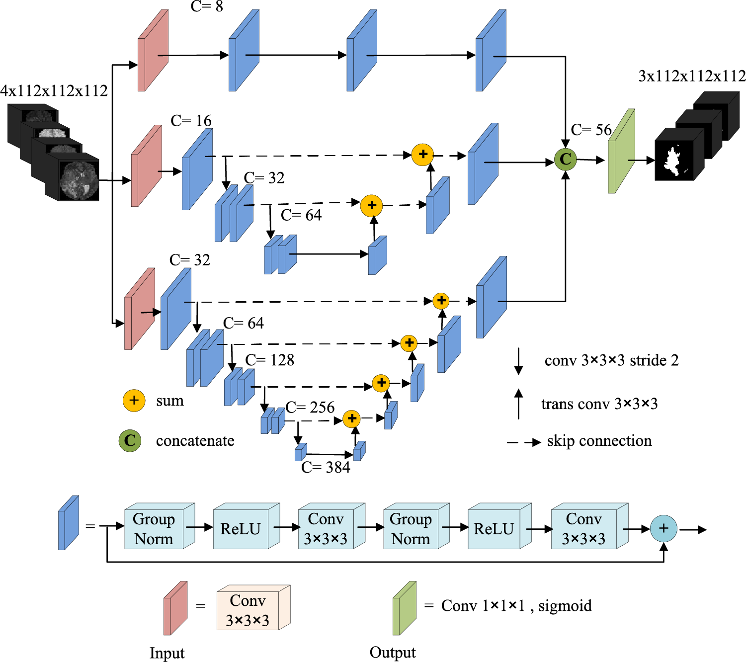
Figure 1: Network architecture

The first branch network is a fully convolution network without down-sampling, which mainly learns the low-level spatial visual information of the image, such as edges, corners, and arcs. This sub-network comprises an input layer (3 × 3 × 3 convolution) and three residual blocks. A dropout layer with a probability of 0.05 is used in the input layer to prevent over-fitting. The number of channels is set to 8 and remains unchanged throughout the convolution process. We do not use down-sampling in this sub-network to preserve the feature scale of the original input image after each convolution, thereby maintaining the high resolution in the learning process. The high-resolution features produced by this sub-network contain more location information, which learns fine-grained information (spatial details like edges, corners, and circles) and is important to predict the tumor position accurately.

The second sub-network is a shallow typical encoding-decoding structure comprising an input layer, three encoding levels, and the corresponding decoding levels. The input layer is a 3 × 3 × 3 convolution with a dropout of probability 0.1 to avoid over-fitting. The first encoding level is a residual block with 16 output channels, and the output scale is the same as the initial scale r. The second and third encoding levels comprise two residual blocks, the channel number increases from 32 to 64, and the feature size decreases from r/2 to r/4. We use a 3 × 3 × 3 strided convolution with stride 2 instead of the pooling layer to keep more important information. In order to fuse the features from different networks efficiently, we use up-sampling operators similar to U-Net to enlarge the feature size. Each spatial level of the decoding pathway has a single residual unit. We use a 3 × 3 × 3 transposed convolution with stride 2 for up-sampling. The feature scale of the top layer of the decoding pathway is the same as the original input scale. Besides, we replaced the concatenation skip connection in the original U-Net with an additional skip connection. Thus, the whole network can be regarded as a residual pattern, and the convolution unit is also a residual block. Therefore, our encoding-decoding architecture is a multi-level residual connection, which strengthens the information propagation, makes the network easier to learn, and accelerates the convergence of the network model. The second sub-network mainly learns the feature information of mid-level object components, which has more semantic information than the output feature map of the first branch network and more spatial information than the output feature map of the third sub-network. Besides, the second sub-network balances semantics and spatiality in the later fusion.

The architecture of the third branch network is similar to the second branch network but deeper than the second one. We use stridden convolution with stride 2 four times to halve the feature scale from the original size r to r/16. As the network depth increases, the receptive field enlarges gradually, and the network learns higher-level semantic information. The channel number of the input layer is 32, doubled after each down-sampling and reaching 512 in the deepest layer. However, there are about 141.5 million parameters, leading the model to overfit and making it challenging to train. Thus, we reduced the number of channels in the fifth layer to 384. The third sub-network learns more high-level semantic feature information, which is helpful for semantic segmentation.

We fuse the outputs of three sub-nets to form feature maps with extensive low-level visual information, mid-level object information, and high-level semantic information, which improves the prediction accuracy of the voxel classification on the MRI images. We use channel concatenation to fuse the outputs of the three sub-networks instead of channel-wise addition to reduce the number of parameters and the loss of information.

The output layer of the network is a 1 × 1 × 1 convolution followed by a sigmoid to generate the final feature for prediction. The number of output channels is 3, representing the segmentation prediction of the whole tumor, tumor core, and enhanced tumor region. Each channel output is a binary classification: background and tumor region.

2.3 Loss Function

The foreground and background voxel distribution in BraTS MRI images suffer from an extreme class imbalance, as 98% of the voxels are background, and only 2% are tumors. Thus, we randomly crop the original image to the patch of size 112 × 112 × 112 as the network input. The patch contains many uninterested regions, leading to a class imbalance in the training data. To alleviate the input class imbalance, Dice loss [29,30], based on region optimization and focal loss [31], is commonly applied in medical image segmentation [14,20,32,33]. There is also an output imbalance problem in deep learning segmentation: the imbalance between false positives (FPs) and false negatives (FNs) during inference. To handle both input and out imbalance, Taghanaki et al. [34] introduced the Combo loss that linearly combines Dice loss for solving input imbalance and modified cross entropy for controlling the trade-off between FP and FN. Combo loss is defined as:

L=αLCE−(1−α)LDice(1)

where LCE is the modified cross-entropy (Eq. (2)), and LDice is the Dice loss (Eq. (3)), which controls the contribution of the Dice loss function to the overall loss function L.

LCE=∑k=1K(−1N∑i=1N[β(tkilnpi)+(1−β)[(1−ti)ln(1−pi)]])(2)

where K is the number of brain tumor region classes set to 3, N is the multiplication of the number of classes and number of samples, ti is the ground truth of voxel i, pi is the predicted probability of voxel i, β ∈ [0,1] controls the trade-off between FN and FP. When β < 0.5, FP is more penalized than FN, and vice versa.

LDice=∑k=1K(2∑i=1Npiti+ε∑i=1Npi+∑i=1Nti+ε)(3)

where ε is the smoothing constant to avoid the numerator and denominator being 0.

3  Experiments, Results, and Discussions

3.1 Implementation Details and Training

The proposed network uses Pytorch and is trained on NVIDIA GeForce RTX 2080 Ti GPU with 11 GB memory. We train the network for 400 epochs, where each epoch contains two patches of size 4 × 112 × 112 × 112 (4 is the MRI modality number) randomly selected from each patient. We use a batch of size 1 and employ the Adam optimizer with an initial learning rate of L0 = 10−4 and an L2 weight decay of 1e-5. The learning rate decreased gradually according to the following formula:

L=L0×(1−eN)0.9(4)

where e is an epoch counter, and N is the total number of epochs (N is 400 in our work).

3.2 Evaluation Metrics

The BraTS dataset provides three labels for training. To evaluate the network model segmentation performances of participants, BraTS organizers divide different brain tumor structures into three overlapping regions: whole tumor (WT, including all regions of labels 1, 2, and 4), tumor core (TC, including regions of labels 1 and 4) and enhancing tumor (ET, region of only label 4). For WT, TC, and ET, the segmentation performance is evaluated based on four metrics: Dice Similarity Coefficient (DSC), Sensitivity, Specificity, and Hausdorff distance (95th percentile) [5]. The DSC assesses the overlapping between the automatic and manual segmentation and is defined as:

DSC(A,M)=2|A∩M||A|+|M|(5)

where A is the tumor region automatically segmented by the model, and M is the manual tumor segmentation. Sensitivity measures the proportion of positive tumors that are correctly predicted:

Sens(A,M)=|A∩M||M|(6)

Specificity calculates the ratio of actual non-tumors that are correctly identified:

Spec(A,M)=|A0∩M0||M0|(7)

where A0 is the non-tumor that is correctly predicted and M0 is manual non-tumor segmentation. Finally, the Hausdorff distance calculates the surface distance between automatically and manually segmented regions, defined as:

Haus(A,M)=max{supinfa∈∂A1,m∈∂M1d(a,m),supinfm∈∂M1,a∈∂A1d(m,a)}(8)

where d(a,m) is the distance between the point a and point m.

3.3 Results and Discussions

3.3.1 The Influence of Multi-Level Branch Networks on Segmentation

Next, we train three sub-networks and multiple combinations of sub-networks on the BraTS 2020 training dataset to quantify the effectiveness of three different level sub-networks on the segmentation performance of the whole network. The prediction results of the validation dataset are uploaded to the BraTS online evaluation tool to obtain the segmentation metrics evaluation value. Table 1 reports the average and sum of DSC of the enhancing tumor (ET), whole tumor (WT), and tumor core (TC) obtained from seven combination networks on the BraTS 2020 validation dataset. We train three sub-networks and find that the deepest branch network has the best segmentation performance, and the sum of Dice for three tumor regions is 2.524. The segmentation performance can be improved after the low-level network is combined with the mid-level and high-level network, especially in the small region target TC and ET. The combination of mid-level and high-level networks has achieved a better effect, revealing that the high-resolution information of the low-level network and mid-level feature information improve tumor segmentation accuracy. The results reveal that fusing the low-level high-resolution information, mid-level object component feature information, and high-level semantic information and forming a multi-level parallel network affords the best segmentation performance for the three region tumors. The total Dice value of the tumor is 2.524, which is 0.56% higher than the segmentation of mid-level and high-level networks.

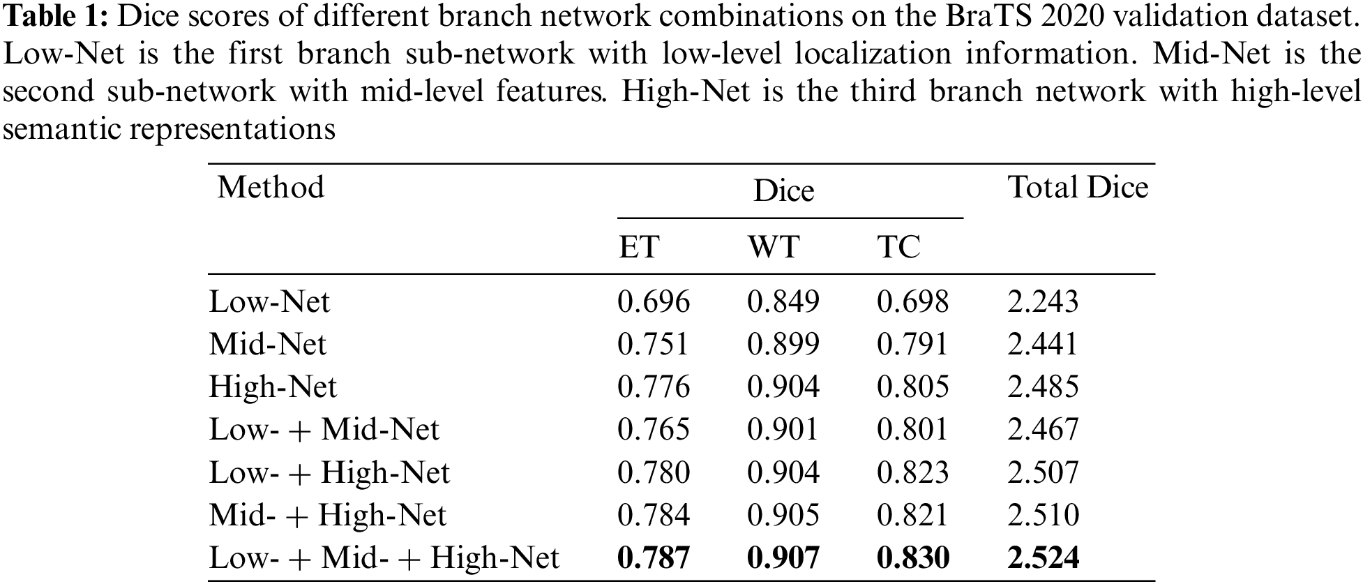
Table 2 reports the mean value of sensitivity, specificity, and Hausdorff95 of different branch networks on the BraTS 2020 validation dataset. Due to the brain image’s large background region, the specificity of all branches is excellent. The network model with three parallel branches has performed best on sensitivity values.

In order to further verify the segmentation performance of the network model, we randomly selected a case (case name: BraTS20_Validation_005) from the validation dataset for qualitative and quantitative analysis. We use five networks (Low-Net, Mid-Net, Hight-Net, Low- + Mid-Net, Low- + Mid- + High-Net) to compare the segmentation results on three different axes: Axial, Coronal, and Sagittal of flair modality, which is depicted in Fig. 2. The three sub-regions segmented by Low- + Mid- + High-Net are the most similar to the target region, and the edge contour lines are also relatively smooth.

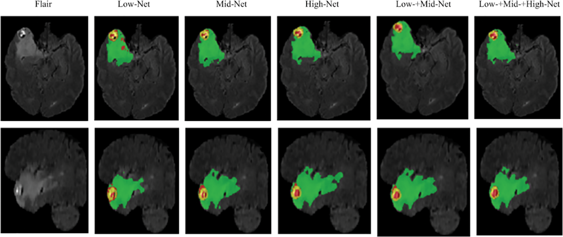
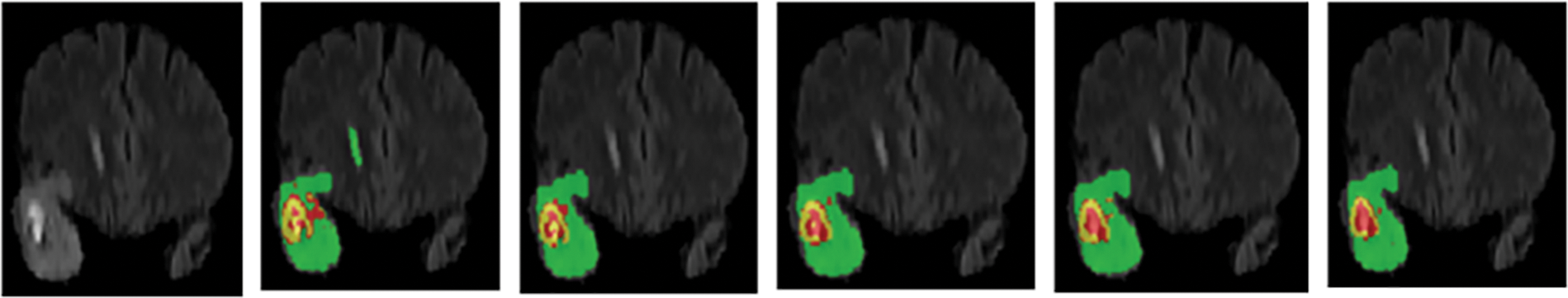
Figure 2: Segmentation of different branch networks in the same case. Green, yellow, and red indicate edema, enhancing tumor core, necrotic, and non-enhancing tumor core regions

To further quantitatively assess the segmentation performance of our method, Table 3 presents the Dice scores of the case BraTS20_Validation _005 using the above five networks on the BraTS 2020 validation dataset. The low-level, mid-level, and high-level sub-networks network achieves excellent Dice scores. The above qualitative and quantitative analysis demonstrates that the proposed multi-level parallel network model is effective for brain segmentation of random individual cases.

3.3.2 The Influence of Loss Function on Segmentation

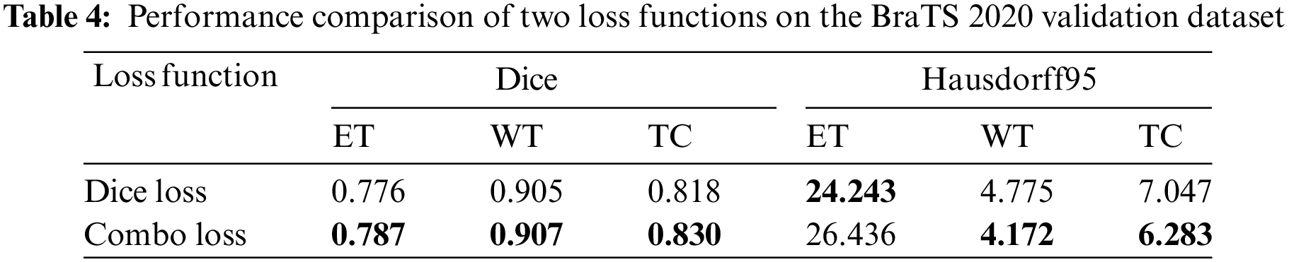
Many brain tumor segmentation networks use Dice loss functions because BraTS uses region-based Dice scores to evaluate segmentation prediction results. However, although the Dice loss function aims to solve the class imbalance problem, there is still an imbalance between false positive and negative samples in the deep learning inference stage. Nevertheless, this paper employs the Combo loss function, simultaneously solving the class imbalance problem and the imbalance between false positive and false negative samples. Table 4 presents the segmentation results of the proposed method using two loss functions. It can be seen that the Combo loss function is better than the Dice loss function in the segmentation performance of the three tumor regions. Because the Combo Loss function punished false positive samples prone to appear in small regions, the segmentation performance of ET and TC has improved significantly. Specifically, ET and TC’s Dice score increased by 1.42% and 1.47%, respectively.

3.3.3 Comparison of Segmentation Results

In order to verify the effectiveness of the proposed network comprehensively, we compare it with other advanced methods qualitatively and quantitatively.

Visual comparison. Fig. 3 visually compares the segmentation results of brain tumors from three cases (from top to bottom: BraTS20_Training_095, BraTS20_Training_170, and BraTS20_Training_233) when using our network and three advanced networks. The segmentation results of three cases show that the 3D U-Net can roughly segment contours of WT and TC regions loosely, but there is misclassification for small region ET. The segmented tumor regions, especially the red ET regions using our method, are closer to the ground truth. In the ground truth tumor regions of case 3, there are very few pixels in the ET region. Our model has the most accurate predictions compared to the other three models, as it can generate feature maps with low-level, mid-level, and high-level information before prediction. Hence, our method accurately predicts the location and classification of tumors, especially small region tumors. In addition, the combo loss function penalizes false positive samples in small regions, improving small tumor region segmentation performance.

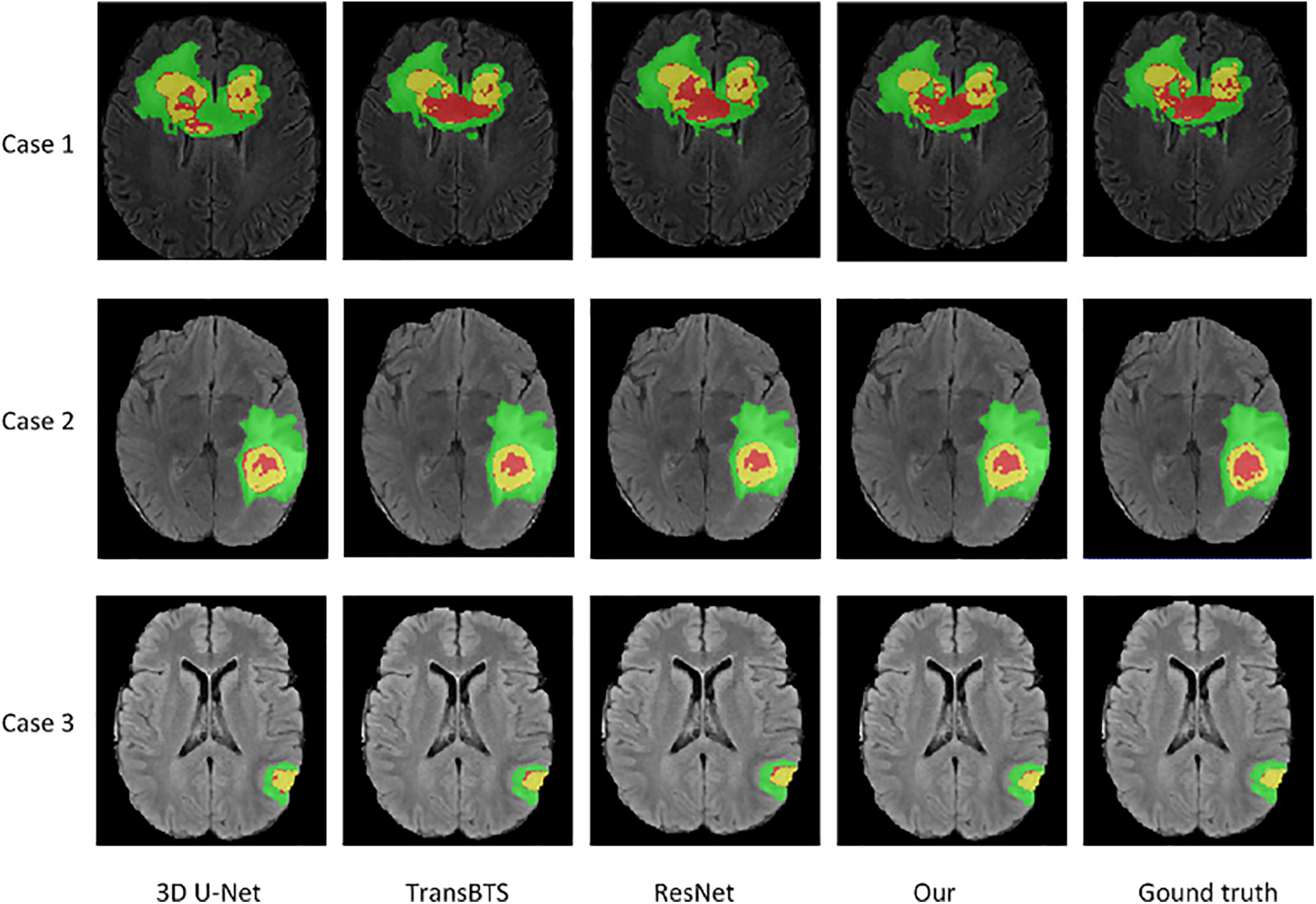
Figure 3: Visualization of segmentation results of brain tumors by our network and three advanced networks. Green, yellow, and red indicate edema, enhancing tumor core, necrotic, and non-enhancing tumor core regions

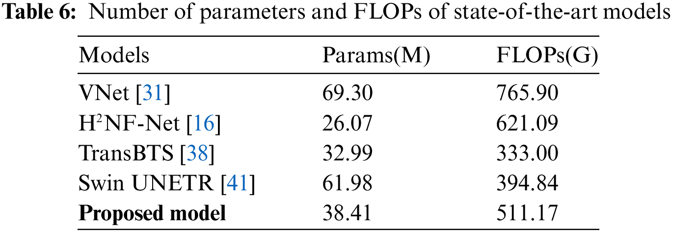
Evaluation metrics comparison. Table 5 compares the proposed method with state-of-the-art methods in the BraTS 2020 challenge on the Dice Similarity Coefficient and Hausdorff distance. The Dice scores of the proposed method for ET, WT, and TC are 0.787, 0.907, and 0.830. Moreover, the Hausdorff95 distances for ET, WT, and TC are 26.47, 4.17, and 6.28, respectively. The ET region, the smallest sub-region, is the most difficult to segment. Compared to the nnU-Net [32] and H2NF-Net [16], which won first and second place in the BraTS 2020 Challenge, respectively, the proposed network obtained a Dice value for ET of 0.787 that is just 0.05 lower than the nnU-Net and 0.001 lower than the H2NF-Net. Besides, the Hausdorff95 distance of ET is 26.47, shorter by 10.4% and 0.38% than the nnU-Net and H2NF-Net, respectively. Our method’s ET Dice score is higher than other state-of-the-art methods, indicating that our proposed method has advantages in edge recognition of small tumor regions. Compared with state-of-the-art methods, our multi-level parallel network achieved competitive performance in the small sub-region target segmentation. From the perspective of network structure, the H2NF-Net comprises five parallel sub-nets with different levels, and although it is superior to the proposed method, it imposes a high computational complexity. Table 6 highlights that H2NF-Net has 621.09 G FLOPs, 21.5% higher than our method. Additionally, our method has obvious advantages over the traditional 3D U-Net [35] because our method can generate feature maps with multi-level information.

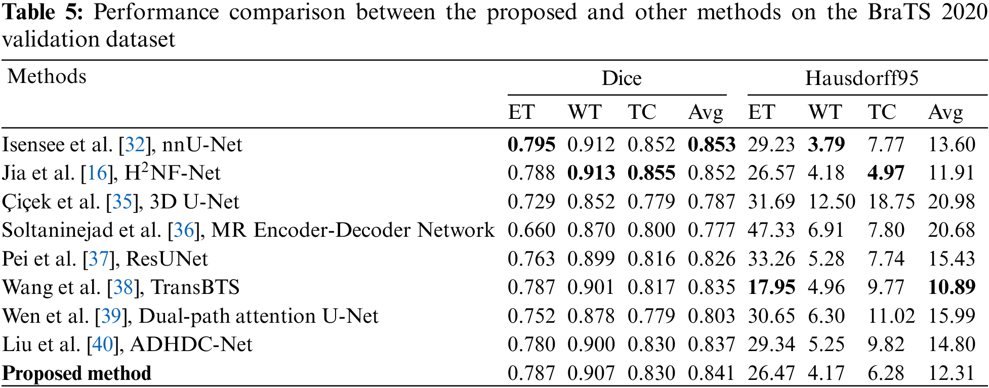
Soltaninejad et al. [36] presented a multi-resolution encoder-decoder network that comprises two branches with different resolution and receptive fields. However, their network did not achieve good results, and the ET Dice score was only 0.66. It is worth noting that our method achieved metric values superior to [36]. Pei et al. [37] proposed a 3D self-ensemble ResUNet deep neural network architecture comprising a regular ResUNet and a self-ensemble model. The loss function uses the traditional Dice loss function without considering the output imbalance problem. We use the Combo loss function to solve the input class and output imbalance problems simultaneously; thus, our method is better than [37]. Self-attention mechanisms have improved the performance of convolutional neural networks in recent years. Wang et al. [38] first adopted Transformer to 3D CNN for brain tumor segmentation and named the network TransBTS, which performs well in small target regions. TransBTS obtained the same Dice value of ET with our method, and the Hausdorff95 value of ET is better than ours, but the other validation metrics are lower than ours. Although TransBTS applied the Transformer into the bottleneck of U-Net, the spatial and time complexity of the Transformer is high, and thus the network’s FLOPs are up to 333 G. Wen et al. [39] proposed a dual-path attention U-Net that fed parallel channel and spatial attention blocks into the skip-connection of U-Net. However, their method’s segmentation performance is unsatisfactory. Liu et al. [40] adopted the attention mechanism to a multiscale 3D U-Net named the network ADHDC-Net, which can improve the segmentation performance of small target regions. The ADHDC-Net achieved a TC Dice value of 0.830, as good as our network, but the Dice values of the smallest ET and the largest WT region and all Hausdorff95 values are lower than our method.

The main reasons why our method obtained competitive results, especially in small tumor regions, are the following: (1) Three serial sub-networks were trained in parallel to exploit abundant low-level, mid-level, and high-level feature information with different numbers of channels, thereby reducing the error of output feature maps and the variance of the network model. (2) We adopted residual blocks to alleviate network degradation and effectively make the second and third sub-network multi-layer residual connection with inner short residual connection and outer long residual connection, strengthening feature propagation and fusing information from multi-level feature maps. (3) A channel-wise concatenation fused the outputs of three branch networks to generate feature maps with rich low-level, mid-level, and high-level information. This strategy reduced the loss of information and accurately predicted the edge or details of brain tumors, thereby improving the performance of small tumor regions. (4) We introduced the Combo loss function, which deals with input class imbalance and output imbalance simultaneously and has good stability for segmenting small region targets.

Due to GPU limitations, the input image block size of our method is 112 × 112 × 112 with a batch size of 1, while the excellent top methods in [32] and [16] have block sizes of 128 × 128 ×128 with training batch sizes of 5 and 4, respectively. We believe increasing the block and batch sizes will further improve our method’s segmentation performance.

Model complexity comparison. Table 6 reports the comparative experiments on model complexity. The proposed network has 38.4 M parameters and 511.17 G FLOPs, which is not a high-size model. In order to reduce the parameters and computational complexity caused by the parallel network structure, we set different initial channel numbers based on the contribution level of sub-networks and reduced the channel number of the deepest scale of the third branch network from the normal doubled number of 512 to 384. Compared with VNet [31] and H2NF-Net [16], the proposed method is superior regarding FLOPs. Generally, parallel networks have many parameters, but our network has only 38.4 M, which is more lightweight than Swin UNETR [41] and VNet [31].

4  Conclusion

This paper proposes a multi-level parallel network architecture, which combines the advantages of parallel and serial network structure. Our architecture comprises three parallel sub-networks, where each is a multiscale serial network structure that mainly learns low-level, mid-level, and high-level feature information. We fuse the outputs of the three sub-networks by using channel concatenate to yield feature maps with abundant multi-level information, predicting accurately the voxels classifies of MRI images. The proposed method is the first fusing information from mid-level object parts for brain tumor segmentation of MRI images, achieving excellent results in small ET regions. In order to efficiently strengthen the propagation of gradients and improve network performance, we employ residual connection in sub-networks and use element-wise skip connection to propagate the short-range and long-range gradients. Additionally, we adopt the Combo loss function for solving input class imbalance and output imbalance in deep learning to improve network performance. Our method obtains Dice scores of 0.787, 0.907, 0.830, and Hausdorff95 distances 26.47, 4.17, and 6.28 for ET, WT and TC, respectively. The experimental results demonstrate that the proposed multi-level parallel network achieves competitive segmentation on the BraTS 2020 dataset, especially in small ET regions, compared to state-of-the-art methods.

However, the parallel network architecture increases computational complexity. Thus, to reduce our network’s complexity, we set different initial channel numbers for three sub-networks with different important levels and reduce the channel number of the deepest layer in the third branch network. Hence, the proposed model balances complexity and performance, but the computational complexity still needs to be optimized compared to other lightweight models.

Acknowledgement: We would like to thank CBICA for providing the BraTS 2020 training dataset, validation dataset, and online validation tools at https://ipp.cbica.upenn.edu/.

Funding Statement: This study was supported by the Sichuan Science and Technology Program (No. 2019YJ0356).

Author Contributions: Study conception and design: Juhong Tie, Hui Peng; data collection: Juhong Tie; analysis and interpretation of results: Juhong Tie and Hui Peng; draft manuscript preparation: Juhong Tie and Hui Peng. All authors reviewed the results and approved the final version of the manuscript.

Availability of Data and Materials: The BraTS 2020 training data and validation data used in the study can be requested at https://ipp.cbica.upenn.edu/. To keep the fairness of BraTS challenge 2020, the BraTS organizer did not release the testing data.

Conflicts of Interest: The authors declare that they have no conflicts of interest to report regarding the present study.

References

1. Zhang, S., Sun, K., Zheng, R., Zeng, H., Wang, S. et al. (2021). Cancer incidence and mortality in China, 2015. Journal of the National Cancer Center, 1(1), 2–11. https://doi.org/10.1016/j.jncc.2020.12.001 [Google Scholar] [CrossRef]

2. Zheng, R., Zhang, S., Zeng, H., Wang, S., Sun, K. et al. (2022). Cancer incidence and mortality in China, 2016. Journal of the National Cancer Center, 2(1), 1–9. https://doi.org/10.1016/j.jncc.2022.02.002 [Google Scholar] [CrossRef]

3. Stupp, R., Taillibert, S., Kanner, A., Read, W., Steinberg, D. et al. (2017). Effect of tumor-treating fields plus maintenance temozolomide vs maintenance temozolomide alone on survival in patients with glioblastoma a randomized clinical trial. JAMA, 318(23), 2306–2316. https://doi.org/10.1001/jama.2017.18718 [Google Scholar] [CrossRef]

4. Goodenberger, M. L., Jenkins, R. B. (2012). Genetics of adult glioma. Cancer Genetics, 205(12), 613–621. https://doi.org/10.1016/j.cancergen.2012.10.009 [Google Scholar] [PubMed] [CrossRef]

5. Menze, B. H., Jakab, A., Bauer, S., Kalpathy-Cramer, J., Farahani, K. et al. (2015). The multimodal brain tumor image segmentation benchmark (BRATS). IEEE Transactions on Medical Imaging, 34(10), 1993–2024. https://doi.org/10.1109/TMI.2014.2377694 [Google Scholar] [PubMed] [CrossRef]

6. Havaei, M., Dutil, F., Pal, C., Larochelle, H., Jodoin, P. M. (2015). A convolutional neural network approach to brain lesion segmentation. Proceedings of MICCAI-BRATS, pp. 29–33. Munich, Germany. [Google Scholar]

7. Pereira, S., Pinto, A., Alves, V., Silva, C. A. (2016). Brain tumor segmentation using convolutional neural networks in MRI images. IEEE Transactions on Medical Imaging, 35(5), 1240–1251. https://doi.org/10.1109/TMI.2016.2538465 [Google Scholar] [PubMed] [CrossRef]

8. Dvorak, P., Menze, B. H. (2015). Structured prediction with convolutional neural networks for multimodal brain tumor segmentation. Proceedings of MICCAI BRATS, pp. 13–24. Munich, Germany. [Google Scholar]

9. Urban, G., Bendszus, M., Hamprecht, F., Kleesiek, J. (2014). Multi-modal brain tumor segmentation using deep convolutional neural networks. Proceedings of MICCAI-BRATS, pp. 31–35. Boston, USA. [Google Scholar]

10. Kamnitsas, K., Ledig, C., Newcombe, V. F. J., Simpson, J. P., Kane, A. D. et al. (2017). Efficient multi-scale 3D CNN with fully connected CRF for accurate brain lesion segmentation. Medical Image Analysis, 36, 61–78. https://doi.org/10.1016/j.media.2016.10.004 [Google Scholar] [PubMed] [CrossRef]

11. Long, J., Shelhamer, E., Darrell, T. (2015). Fully convolutional networks for semantic segmentation. Proceedings of IEEE Conference on Computer Vision and Pattern Recognition (CVPR), pp. 3431–3440. Boston, MA, USA. [Google Scholar]

12. Ronneberger, O., Fischer, P., Brox, T. (2015). U-Net: Convolutional networks for biomedical image segmentation. Medical Image Computing and Computer-Assisted Intervention, 9351, 234–241. [Google Scholar]

13. Myronenko, A. (2019). 3D MRI brain tumor segmentation using autoencoder regularization. Proceedings of BrainLes MICCAI, pp. 311–320. Granada, Spain. https://doi.org/10.1007/978-3-030-11726-9_28 [Google Scholar] [CrossRef]

14. Isensee, F., Kickingereder, P., Wick, W., Bendszus, M., Maierhein, K. H. (2019). No New-Net. Proceedings of 7th MICCAI BraTS Challenge, pp. 222–231. Granada, Spain. https://doi.org/10.1007/978-3-030-11726-9_21 [Google Scholar] [CrossRef]

15. Jiang, Z., Ding, C., Liu, M., Tao, D. (2020). Two-stage cascaded U-Net: 1st place solution to BraTS challenge 2019 segmentation task. Proceedings of International MICCAI Brainlesion Workshop, pp. 231–241. Shenzhen, China. https://doi.org/10.1007/978-3-030-46640-4_22 [Google Scholar] [CrossRef]

16. Jia, H., Xia, Y., Cai, W., Huang, H. (2021). H2NF-net for brain tumor segmentation using multimodal MR imaging: 2nd place solution to BraTS challenge 2020 segmentation task. Proceedings of International Conference on Medical Image Computing and Computer-Assisted Intervention (MICCAI), pp. 56–85. Lima, Perul. https://doi.org/10.1007/978-3-030-72087-2_6 [Google Scholar] [CrossRef]

17. Chang, Y., Zheng, Z., Sun, Y., Zhao, M., Lu, Y. (2023). DPAFNet: A residual dual-path attention-fusion convolutional neural network for multimodal brain tumor segmentation. Biomedical Signal Processing and Control, 79, 104307. https://doi.org/10.1016/j.bspc.2022.104037 [Google Scholar] [CrossRef]

18. Lu, Y., Chang, Y., Zheng, Z., Sun, Y., Zhao, M. et al. (2023). GMetaNet: Multi-scale ghost convolutional neural network with auxiliary MetaFormer decoding path for brain tumor segmentation. Biomedical Signal Processing and Control, 83, 104694. https://doi.org/10.1016/j.bspc.2023.104694 [Google Scholar] [CrossRef]

19. Kamnitsas, K., Bai, W., Ferrante, E., McDonagh, S., Sinclair, M. et al. (2018). Ensembles of multiple models and architectures for robust brain tumor segmentation. Proceedings of the 6th MICCAI BraTS Challenge, pp. 135–146. Quebec City, Canada. https://doi.org/10.1007/978-3-319-75238-9_38 [Google Scholar] [CrossRef]

20. Szegedy, C., Liu, W., Jia, Y., Sermanet, P., Reed, S. et al. (2015). Going deeper with convolutions. Proceedings of IEEE Conference on Computer Vision and Pattern Recognition (CVPR), pp. 1–9. Boston, MA, USA. [Google Scholar]

21. He, K., Zhang, X., Ren, S., Sun, J. (2015). Spatial pyramid pooling in deep convolutional networks for visual recognition. https://arxiv.org/pdf/1406.4729.pdf [Google Scholar]

22. Chen, L., Papandreou, G., Kokkinos, I., Murphy, K., Yuille, A. L. (2018). DeepLab: Semantic image segmentation with deep convolutional nets, atrous convolution, and fully connected CRFs. IEEE Transactions on Pattern Analysis and Machine Intelligence, 40(4), 834–848. https://doi.org/10.1109/TPAMI.2017.2699184 [Google Scholar] [PubMed] [CrossRef]

23. Zhao, H., Shi, J., Qi, X., Wang, X., Jia, J. (2017). Pyramid scene parsing network. Proceedings of IEEE Conference on Computer Vision and Pattern Recognition (CVPR), pp. 6230–6239. Honolulu, HI, USA. [Google Scholar]

24. Lin, G., Liu, F., Milan, A., Shen, C., Reid, L. RefineNet: Multi-path refinement networks for dense prediction. Proceedings of IEEE Conference on Computer Vision and Pattern Recognition (CVPR), pp. 5168–5177. Honolulu, HI, USA. [Google Scholar]

25. Xu, Y., Gong, M., Fu, H., Tao, D., Zhang, K. et al. (2019). Multi-scale masked 3-D U-net for brain tumor segmentation. Proceedings of International MICCAI Brainlesion Workshop, pp. 222–233. Shenzhen, China. https://doi.org/10.1007/978-3-030-11726-9_20 [Google Scholar] [CrossRef]

26. Chen, C., Liu, X., Ding, M., Zheng, J., Li, J. (2019). 3D dilated multi-fiber network for real-time brain tumor segmentation in MRI. Proceedings of International Conference on Medical Image Computing and Computer-Assisted Intervention, pp. 184–192. Shenzhen, China. https://doi.org/10.1007/978-3-030-32248-9_21 [Google Scholar] [CrossRef]

27. Bakas, S., Akbari, H., Sotiras, A., Bilello, M., Rozycki, M. et al. (2017). Advancing the cancer genome atlas glioma MRI collections with expert segmentation labels and radiomic features. Scientific Data, 4, 170117. https://doi.org/10.1038/sdata.2017.117 [Google Scholar] [PubMed] [CrossRef]

28. Bakas, S., Reyes, M., Jakab, A., Bauer, S., Rempfler, M. et al. (2018). Identifying the best machine learning algorithms for brain tumor segmentation, progression assessment, and overall survival prediction in the BRATS challenge. https://arxiv.org/abs/1811.02629 [Google Scholar]

29. He, K., Zhang, X., Ren, S., Sun, J. (2016). Deep residual learning for image recognition. Proceedings of IEEE Conference on Computer Vision and Pattern Recognition (CVPR), pp. 770–778. Las Vegas, NV, USA. [Google Scholar]

30. Tie, J., Peng, H., Zhou, J. (2021). MRI brain tumor segmentation using 3D U-Net with dense encoder blocks and residual decoder blocks. Computer Modeling in Engineering & Sciences, 128(2), 427–445. https://doi.org/10.32604/cmes.2021.014107 [Google Scholar] [CrossRef]

31. Milletari, F., Navab, N., Ahmadi, S. (2016). V-Net: Fully convolutional neural networks for volumetric medical image segmentation. Proceedings of International Conference on 3D Vision, pp. 565–571. Stanford, CA, USA. https://doi.org/10.1109/3DV.2016.79 [Google Scholar] [CrossRef]

32. Isensee, F., Jager, P. F., Full, P. M., Vollmuth, P., Hein, K. H. M. (2020). nnU-Net for brain tumor segmentation. http://arxiv.org/abs/2011.00848 [Google Scholar]

33. Lin, T. Y., Goyal, P., Girshick, R., He, K., Dollar, P. et al. (2017). Focal loss for dense object detection. IEEE Transactions on Pattern Analysis & Machine Intelligence, 42(2), 318–327. https://doi.org/10.1109/TPAMI.2018.2858826 [Google Scholar] [PubMed] [CrossRef]

34. Taghanaki, S. A., Zheng, Y., Zhou, S. K., Georgescu, B., Sharma, P. et al. (2019). Combo loss: Handling input and output imbalance in multi-organ segmentation. Computer Medical Imaging and Graphics, 75, 24–33. https://doi.org/10.1016/j.compmedimag.2019.04.005 [Google Scholar] [PubMed] [CrossRef]

35. Çiçek, Ö., Abdulkadir, A., Lienkamp, S. S., Brox, T., Ronneberger, O. (2016). 3D U-Net: Learning dense volumetric segmentation from sparse annotation. Proceedings of International MICCAI Brainlesion Workshop, pp. 424–432. Athens, Greece. https://doi.org/10.1007/978-3-319-46723-8_49 [Google Scholar] [CrossRef]

36. Soltaninejad, M., Pridmore, T., Pound, M. (2021). Efficient MRI brain tumor segmentation using multi-resolution encoder-decoder networks. Proceedings of International MICCAI Brainlesion Workshop, pp. 30–39. Lima, Peru. https://doi.org/10.1007/978-3-030-72087-2_3 [Google Scholar] [CrossRef]

37. Pei, L., Murat, A. K., Colen, R. (2021). Multimodal brain tumor segmentation and survival prediction using a 3D self-ensemble ResUNet. Proceedings of International MICCAI Brainlesion Workshop, pp. 367–375. Lima, Peru. https://doi.org/10.1007/978-3-030-72084-1_33 [Google Scholar] [CrossRef]

38. Wang, W., Chen, C., Ding, M., Yu, H., Zha, S. et al. (2021). Transbts: Multimodal brain tumor segmentation using transformer. Proceedings of International MICCAI Brainlesion Workshop, pp. 109–119. Lima, Peru. https://doi.org/10.1007/978-3-030-87193-2_11 [Google Scholar] [CrossRef]

39. Wen, J., Xu, H., Zhang, W. (2021). Brain tumor segmentation using dual-path attention U-Net in 3D MRI images. Proceedings of International MICCAI Brainlesion Workshop, pp. 183–193. Lima, Peru. https://doi.org/10.1007/978-3-030-72084-1_17 [Google Scholar] [CrossRef]

40. Liu, H., Huo, G., Li, Q., Guan, X., Tseng, M. L. (2023). Multiscale lightweight 3D segmentation algorithm with attention mechanism: Brain tumor image segmentation. Expert Systems with Applications, 214, 119166. https://doi.org/10.1016/j.eswa.2022.119166 [Google Scholar] [CrossRef]

41. Hatamizadeh, A., Nath, V., Tang, Y., Yang, D., Roth, H. et al. (2022). Swin UNETR: Swin transformers for semantic segmentation of brain tumors in MRI images. Proceedings of International MICCAI Brainlesion Workshop, pp. 272–284. Strasbourg, France. https://doi.org/10.1007/978-3-031-08999-2_22 [Google Scholar] [CrossRef]