Prediction and Output Estimation of Pattern Moving in Non-Newtonian Mechanical Systems Based on Probability Density Evolution

1  Introduction

There is a class of complex industrial processes in modern production processes, such as the sintering process, blast furnace combustion process, and cement rotary kiln production process. Due to their distribution characteristics, nonlinearity, time variation, and parameter perturbation, their dynamic characteristics cannot be accurately described. Moreover, the motion characteristics controlled by statistical laws are common in these complex production processes, and they are collectively referred to as non-Newtonian mechanical systems [1]. Due to the essence of the physical and chemical processes governed by statistical laws in non-Newtonian mechanical systems, the uncertainty of system output is high. Therefore, the operating rules of the system are difficult to describe through traditional mathematical models. For systems with known structural types, the nonlinear model of the system was obtained in [2] by computing the input-output cross-covariance function and the output covariance function. Reference [3] divided the system input and output into a series of subregions and formed the logical composite of time sequences, which were then analyzed by time sequence analysis methods. The aluminum calcination rotary kiln is a typical industrial production process that involves non-Newtonian mechanics. In [4], fuzzy clustering method was used to obtain pattern categories of different operating conditions in the rotary kiln reaction process, and corresponding controllers were designed according to different operating conditions. Therefore, for these types of systems, it is common practice to use approximation methods to partially mathematically describe the system, focusing on solving the identification of the mathematical model structure or system movement state of the system. However, under the control of statistical laws, the output of non-Newtonian mechanical systems is usually uncertain values within the corresponding distribution region. Traditional fitting methods usually only determine the trend of the system, but are difficult to accurately predict the system output. This problem becomes more apparent when the statistical characteristics included in the system become more prominent. Therefore, considering the statistical characteristics of the system, the method for solving the output prediction problem of non-Newtonian mechanical systems can be found by analyzing the changes of the probability density. In addition, since systems involving non-Newtonian mechanical processes generally have significantly different operating conditions, it is common practice to use pattern recognition technology to classify the system into operating condition categories. As early as the early 1960s, pattern recognition technology received attention from the control community. According to [5], a slowly changing stochastic process was divided into multiple regions, and each region was considered as a working condition under the related system characteristics conditions. Then, pattern recognition technology was used to identify the working conditions and design the corresponding system controller. According to [6], the application of pattern recognition technology in controlled systems first requires the establishment of the feature space of the system. Then, the mapping relationship between the feature space and the decision space is established. Finally, pattern recognition technology is used to determine the decision space to which the system belongs, and analyze or design a system controller based on the result. Early on, the analysis and research of controlled systems using pattern recognition technology mainly focused on solving the problem of mathematical model structure identification or system motion state recognition. However, for cases such as non-Newtonian mechanical systems that are difficult to describe through mathematical and physical equations, this method of essentially establishing a corresponding mathematical model according to the pattern category to which the system belongs is powerless.

Recently, a dynamic pattern recognition method has been proposed for systems governed by statistical regularities [7]. The main idea is to map the temporal variation process of the operational conditions of the system to the temporal movement process of the pattern categories to which the operational conditions belong, treating the pattern category as a variable. Unlike deterministic variables such as state variables, the pattern category variable constructed in this way has statistical properties. However, due to the lack of arithmetic properties in pattern category variables, it is necessary to construct a mapping relationship between the pattern category space and the computable space to which it belongs. Currently, a series of achievements have been made in metric methods such as category centers [8–10], interval numbers [11,12], and cell maps [13]. Using category center measurement of pattern category variables is a more intuitive approach. That is, selecting category center points and mapping them to the computable space, and then using traditional control theory and related analysis methods to predict and control system design. The classification mapping is returned to the pattern movement space to form a motion trajectory in the pattern movement space. Although the category center measurement method is more intuitive and operationally simple, the calculation method using the category center is difficult to reflect the statistical properties of the pattern category variable. Therefore, the measurement methods of interval numbers and cell maps actually consider measuring the pattern category variable using an interval range, with the aim of endowing the pattern category variable with statistical properties, while ensuring its statistical properties as much as possible. To endow the category center measurement method with a certain statistical property, a method based on an explicit-implicit mixture measurement method based on category centers was proposed in [14,15], which takes the category center of the current system operating conditions as the explicit measurement value, and other unknown points belonging to the current pattern category as the implicit measurement value. The purpose is to reflect the internal difference characteristics of the pattern category variable. Based on this, the corresponding autoregressive model construction and adaptive control scheme were studied. Analysis of the existing pattern movement-based modeling and control schemes shows that the current theory for the prediction problem of pattern category variables is basically based on the analysis of deterministic variables. For non-Newtonian mechanical systems governed by statistical regularities, their output are essentially random variables, so studying the analysis and prediction problems of pattern movement-based systems from the perspective of random system dynamics analysis is a viable approach.

Non-Newtonian mechanical systems can essentially be considered as a type of special random system. There are two main research routes for the dynamic analysis of stochastic systems: one is the stochastic differential equation research route formed by combining Einstein’s dissipation diffusion relationship with Ito differential equations [16,17], and the other is the statistical analysis methods gradually generated with the development of statistics, mainly including Monte Carlo simulation [18], importance sampling [19,20], and Bayesian methods [21–23]. In recent years, with the study of the probability density conservation principle, a probability density evolution method has been proposed [24,25]. This method constructs the probability density evolution equation of the system based on the probability density conservation principle and then obtains the time-varying probability density function of the stochastic structural response, providing a new approach for the analysis of stochastic dynamic response. It has been successfully applied to the analysis of stochastic dynamic response and reliability analysis of structures under dynamic loads [26]. In recent years, the probability density evolution method has been further applied and developed in many fields, such as reliability analysis and seismic analysis of complex structures. Reference [27] proposed an enhanced probability density evolution method for the reliability analysis of multiple failure modes and limit states, and compared it with Monte Carlo simulation method. The results showed that the enhanced probability density evolution method can reduce computational burden at the same accuracy. Reference [28] integrated the probability density evolution method into the performance-based earthquake engineering for hazard-fragility assessment, proposed a consistent seismic hazard and fragility framework considering combined capacity-demand uncertainties, and verified the accuracy of this method. Reference [29] applied the probability density evolution method to the seismic assessment of concrete dams under consideration of time-varying factors. In addition, Fan et al. [30] derived the generalized probability density evolution equation for degraded structures, and extended the probability density evolution method to the analysis of deteriorating structures with inspection by combining the Bayesian updating process. However, the probability density evolution method is an analytical method in the field of mechanics, and its application in the field of control is relatively rare. In addition, the probability density evolution equation constructed by this method usually needs to be established on the basis of the mathematical equations of the system, which is disadvantageous for complex systems that are difficult to express with mathematical models in the control field. But from the theoretical achievements of probability density evolution method, as a convenient and efficient stochastic analysis method, it can be extended to the field of control to solve problems that are difficult to handle by deterministic variables.

For a controlled system, the data that can usually be obtained is the system’s input-output data. In recent years, a non-parametric dynamic linearization method based on input-output data has been developed [31]. This method mainly constructs a data model that is virtually equivalent to the original system through PPD, and updates it through online data. After more than ten years of development, this method has formed a relatively complete theoretical framework system [32,33]. Traditional non-parametric dynamic linearization methods based on PPD usually do not consider the existence of unmodeled dynamics in the system. One major drawback of this is that sometimes the PPD cannot be effectively estimated due to the system’s nonlinear complexity. To address this problem, articles [34,35] constructed a dynamic linearization method based on ESO by treating unmodeled dynamics as extended states. Overall, the non-parametric dynamic linearization method based on PPD has nice fitting characteristics for the system and does not require a training process. This method can be considered for analyzing non-Newtonian mechanical systems governed by statistical laws.

In conclusion, this work addresses the problem of predicting and analyzing non-Newtonian mechanical systems in literature [1], by taking into account the statistical properties of the system description based on pattern category variables in literature [7], the advantages of the probability density evolution method for analyzing the time evolution of stochastic dynamical systems presented in literature [24], the data-driven characteristic of the non-parametric dynamic linearization proposed in literature [31], and the advantages of processing uncertainty through ESO presented in literature [35]. Based on these considerations, a data-driven approach for predicting and analyzing non-Newtonian mechanical systems is constructed using pattern motion probability density evolution.

Firstly, a model of motion system dynamics based on posterior probability density measurement is proposed. Historical data is collected to form a detection sample sequence, and feature extraction and pattern classification are performed to classify similar operating conditions into categories and construct pattern category variables. When the current output of the system is obtained, the system’s pattern category can be discriminated by pattern classification. Then, the posterior probability is used as the measurement of the pattern category variables and mapped to probability space. The law of probability density evolution is analyzed through the principle of probability density conservation in probability space, and a prediction framework of probability density is constructed. As the evolution of probability density in probability space corresponds to the variation of pattern category variables in motion pattern space, a motion trajectory is ultimately formed in motion pattern space over time.

Then, in order to predict and analyze the probability density evolution of pattern motion, a data-driven algorithm for predicting the probability density evolution of pattern motion is proposed based on the characteristics of non-Newtonian mechanical systems that are difficult to describe through mathematical equations. By constructing PPD, the system is transformed into a data-driven form that includes statistical feature terms. Then, the corresponding probability density evolution equation is constructed through probability density evolution theory, and the probability density prediction is finally achieved based on the current input/output of the system.

Finally, to realize the non-parametric dynamic linearization method with the statistical feature term proposed in this paper, a PPD online estimation algorithm is presented, taking advantage of the structure of the ESO. The statistical feature term is used as the extended state, and the statistical feature term in the PPD estimation law is replaced by the output of the ESO. The boundedness of the proposed PPD estimation algorithm and the boundedness of the evolution prediction of the probability density of pattern motion for system output estimation are theoretically analyzed and numerically demonstrated.

This article provides a new theoretical framework for the analysis of patterned motion in non-Newtonian mechanical systems. Unlike previous methods that measure using pattern category centers, the posterior probability density better reflects the statistical properties of the pattern category variable. This paper combines the system analysis theory in the control field with the probability density evolution theory in the area of stochastic structural dynamics analysis. This provides a solution to the difficulty in estimating outputs in non-Newtonian mechanical systems due to being governed by statistical laws.

The rest of the paper is arranged as follows. Section 2 analyzes the characteristics of non-Newtonian mechanical systems and constructs a dynamic description method based on pattern motion. Section 3 designs a probability density evolution prediction algorithm based on pattern motion and implements system output estimation. Section 4 constructs a PPD estimation law based on ESO and theoretically proves the boundedness of the estimation algorithm, as well as the boundedness the boundedness of the system output estimation designed in Section 3. Section 5 verifies the proposed theory through numerical simulation. Section 6 provides a corresponding summary of the work in this paper.

2  Problem Description

2.1 Non-Newtonian Mechanical Systems

For a class of complex industrial production systems governed by statistical regularities, it is considered that they share the following three common features:

1)   The production process involves complicated technological procedures, and its motion mechanism cannot be fully explained at the current stage. During the system’s operation, a series of intertwined physico-chemical changes include combustion thermodynamics, chemical reaction kinetics, phase transitions, and moving boundaries, making it challenging to use existing mathematical and physical equations for description.

2)   The system motion exhibits complex characteristics such as distributed characteristics, nonlinearity, and time-varying parameters.

3)   Some physical processes in the system essentially conform to the laws of statistical movement, such as the physical transformation from liquid phase to solid phase, granularity and fluidity. The corresponding relationships between many variables that characterize operating conditions and product quality cannot be described through deterministic mathematical equations, and only exist in a statistical sense. System dynamics are essentially not governed by Newtonian mechanics but by statistical laws.

It is precisely the characteristic of being governed by statistical regularities that distinguishes these types of systems from other general nonlinear systems and is thus referred to as non-Newtonian mechanical systems [1]. The aforementioned features indicate that the output of non-Newtonian mechanical systems is not a deterministic variable, which poses significant challenges for the traditional state variable-based system dynamic description.

2.2 Dynamic Description Method Based on Pattern Motion

Assuming that a non-Newtonian mechanical system that satisfies the characteristics 1) to 3) can be represented in the form of formula (1).

y(k+1)=f(y(k),y(k−1),⋯,y(k−n),u(k),u(k−1),⋯,u(k−m))+ω(k)(1)

where, f(⋯) represents an unknown nonlinear function, n and m are two unknown positive integers, and ω(k) is a random variable with probability density pd(ω).

Remark 1: The system represented by formula (1) is different from general nonlinear systems. In general nonlinear systems, ω is usually a perturbation that has limited influence on the system. However, in this paper, it represents a non-Newtonian mechanics system governed by statistical regularities, and ω is a random variable that characterizes the statistical properties of the system itself. External perturbations to the system are naturally included, so ω has an equally important impact on the system compared to its nonlinear component f(⋯). Additionally, the presence of ω results in the system’s output being an uncertain quantity governed by statistical regularities, making it difficult to predict the system’s output.

According to the analysis of the system (1), it is difficult to describe and predict its output using traditional mathematical model structures due to it being a stochastic variable governed by statistical laws. This paper draws on the research results of pattern recognition, and the method of pattern recognition is used to classify system output samples with similar or identical operating conditions into a pattern category, in order to construct a pattern category variable and describe the system’s motion law using the pattern category variable instead of the state variable.

For a complex industrial production process, input and output data are continuously collected over a sufficient period of time to form a data space. If the data sample is large enough, the information reflecting the motion characteristics of the system can be covered, and it can be considered that the motion of the production process should operate within this data space. This data space is called the motion subspace of the industrial production process. Feature variables are extracted from data on the motion subspace to obtain a pattern sample sequence containing the main statistical characteristics, and the space formed by the feature variables is called the feature variable subspace. The pattern recognition method is used to classify the feature variable subspace, and the pattern categories obtained serve as spatial scales. When the current state data of the system is obtained, the system state can be directed to the corresponding pattern category scale through feature extraction and classification operations. The construction of the pattern category variable is as follows:

Definition 1: Let {Sx(k)} and {Mx(k)} represent the detection sample sequence and pattern sample sequence, respectively. T(⋅) and F(⋅) represent the feature extraction and classification processes, respectively. After the detection sample undergoes the feature extraction process, a pattern sample sequence that characterizes the motion characteristics of the system is obtained. The pattern sample is then classified by a classifier to obtain a pattern category variable with category information:

Mx(k)=T(Sx(k))I(k)=F(Mx(k))(2)

Remark 2: According to Definition 1, the pattern category variable is a function of time and has categorical and statistical properties. Furthermore, the construction process of the pattern category variable shows that it does not satisfy the calculation rules of Euclidean space and needs to be endowed with computable attributes through metric mapping. In addition, the construction process described in definition 1 indicates that the construction of pattern category variables requires the collection of sufficient system output samples, and then analyzing the common characteristics between output samples through pattern recognition methods such as clustering, and grouping samples with the same statistical characteristics into the same pattern category.

According to Definition 1 and Remark 2, the pattern category variable is constructed from working condition samples with the same or similar attributes. Therefore, there must be a corresponding distribution relationship between the various categories corresponding to the pattern category variable and the system data. In other words, different categories have their own class conditional probability density. Estimating the class conditional probability density for each category based on historical working condition data is actually a typical non-parametric estimation problem. It can be estimated using non-parametric estimation methods such as Parzen windows. For the non-Newtonian mechanical system shown in formula (1), the corresponding pattern categorical variable is constructed according to Definition 1. In order to endow the pattern categorical variables with computable properties while ensuring the statistical properties of it, the class conditional probability density is used to measure it. The pattern motion dynamics description of system (1) based on conditional probability density measurement is as follows:

y(k+1)=f(y(k),y(k−1),⋯,y(k−n),u(k),u(k−1),⋯,u(k−m))+ω(k)I(k)=F(y(k))p(y(k)|I(k))=D(I(k))(3)

where, D(⋅) is a measure mapping of pattern category variables, I(k) is a sequence of pattern category variables that ends at time k, I(k)={I(i):i=1,2,⋯,k}, and p(y(k)|I(k)) is the class conditional probability density, which is essentially a posterior probability density.

3  Prediction of Pattern Motion Probability Density Evolution and Output Estimation

From the description of pattern motion dynamics based on conditional probability density measurements (3), it can be realized that in order to predict the output pattern category variables of non-Newtonian mechanical systems, it is necessary to analyze the changing rules of corresponding posterior probability density p(y(k)|I(k)) with time. According to formula (1), the randomness of the system comes solely from the random variable ω(k), and no new random factors intervene during the time period under consideration. Therefore, based on the probability density conservation principle, the class conditional probability density corresponding to the pattern category variable must be conserved. The following generalized probability density evolution equation can be constructed.

∂pYΩ(y,ω(k)|I)∂t+y˙(t)∂pYΩ(y,ω(k)|I)∂y=0(4)

where, pYΩ(y,ω(k)|I) is the joint conditional probability density of system outputs y and ω(k) under the condition of historical pattern category sequence I. It is known from the generalized probability density evolution equation that the solution of the equation requires the comprehensive speed y˙(t) of all sample state changes of the system, namely, the physical answer of the system equation [24].

However, the system equation of the non-Newtonian mechanical system studied in this paper is difficult to obtain. Therefore, the comprehensive speed y˙(t) is also difficult to obtain. Based on this analysis, the concept of PPD is used to construct a data-driven form of the probability density evolution prediction model.

The main idea is to construct corresponding data-driven expression by input-output data of the system in real-time, and then replace the system equations in formula (3) with the data-driven expression. At this point, the generalized probability density evolution equation shown in formula (4) can also be rewritten into a corresponding data-driven format, and the prediction of the conditional probability density of the pattern category can be solved. The construction of the data-driven expression of the non-Newtonian mechanics system based on PPD is given by Theorem 1, and the corresponding data-driven format of the generalized probability density evolution and the prediction method of the conditional probability density of the pattern class is given by Theorem 2.

To facilitate the analysis and research of the system, the following two assumptions are made for system (1).

Assumption 1: The non-Newtonian mechanical system (1) under consideration satisfies the generalized Lipschitz condition, that is, for all k except finite exceptions, if any k1≠k2, k1,k2⩾0 and u(k1)≠u(k2) are satisfied, it can be obtained that:

|y(k1+1)−y(k2+1)|⩽b|u(k1)−u(k2)|(5)

where, y(ki+1)=f(y(ki),⋯,y(ki−n),u(ki),⋯,u(ki−m)),i=1,2, b is a constant and b>0.

Assumption 2: Except for the finite time point, the partial derivative of f(⋯) with respect to the (n + 2)th variable is continuous.

Remark 3: From the perspective of practical systems, it is reasonable to add the two assumptions to the system (1). Assumption 1 imposes an upper limit on the rate of change of the system output in response to changes in the system input. In fact, if the changes in the control inputs remain within a limited range, the changes in the system output cannot reach infinity. This assumption is satisfied by many practical systems. Assumption 2 is a typical constraint in the design of nonlinear control systems.

Theorem 1: For a non-Newtonian mechanical system (1) that satisfies Assumptions 1 and 2, when |Δu(k)|≠0, there exists a time-varying parameter φ(k)∈R referred to as pseudo partial derivative that transforms the system into a compact format dynamic linearized data model, and |φ(k)|≤b holds for any time k.

Δy(k+1)=φ(k)Δu(k)+ζ(k)(6)

where, Δy(k+1)=y(k+1)−y(k), Δu(k)=u(k)−u(k−1), ζ(k)=ω(k)−ω(k−1), and the probability density of ζ satisfies pZ(ζ)=∫Ωωpd(ω)pd(ω−ζ)dω.

Remark 4: φ(k) and ζ(k) are two time-varying functions, although they are represented in the form of time-varying parameters.

Proof: Consider the non-Newtonian mechanical system shown in formula (1), from Δy(k+1)=y(k+1)−y(k), then:

Δy(k+1)=y(k+1)−y(k)=f(y(k),y(k−1),⋯,y(k−n),u(k),⋯,u(k−m))+ω(k)−f(y(k−1),y(k−1),⋯,y(k−n−1),u(k−1),⋯,u(k−m−1))−ω(k−1)=f(y(k),y(k−1),⋯,y(k−n),u(k),⋯,u(k−m))+ω(k)−f(y(k),⋯,y(k−n),u(k−1),⋯,u(k−m))+f(y(k),⋯,y(k−n),u(k−1),⋯,u(k−m))−f(y(k−1),y(k−2),⋯,y(k−n−1),u(k−1),⋯,u(k−m−1))−ω(k−1)(7)

According to Cauchy mean value theorem, there must be a point in [y(k),⋯,y(k−n),u(k−1),⋯,u(k−m)]T, so that the partial derivative ∂f∗∂u(k) of f(⋯) relative to the (n + 2)th variable has:

f(y(k),y(k−1),⋯,y(k−n),u(k),⋯,u(k−m))−f(y(k),y(k−1),⋯,y(k−n),u(k−1),⋯,u(k−m))=∂f∗∂u(k)Δu(k)(8)

Let:

Ψ(k)=f(y(k),⋯,y(k−n),u(k−1),⋯,u(k−m))−f(y(k−1),⋯,y(k−n−1),u(k−1),⋯,u(k−m−1))(9)

There exists the following equation for each determined time k on [y(k),⋯,y(k−n),u(k),⋯,u(k−m)]T:

Ψ(k)=η(k)Δu(k)(10)

Since |Δu(k)|≠0, the above equation must have a unique solution η∗(k). Substituting formulas (8) and (10) into formula (7) yields:

Δy(k+1)=(η∗(k)+∂f∗∂u(k))⋅Δu(k)+ω(k)−ω(k−1)(11)

Let φ(k)=η∗(k)+∂f∗∂u(k), ζ(k)=ω(k)−ω(k−1), Then formula (11) can be rewritten as:

Δy(k+1)=φ(k)Δu(k)+ζ(k)(12)

For ζ(k) in formula (12), according to the definition of probability density, its probability density is:

pZ(ζ(k))=limh→0(P(Z∈[ζ(k),ζ(k)+h])/h)(13)

Substituting ζ(k)=ω(k)−ω(k−1) into formula (13) can further transform it into the form shown in formula (14):

pZ(ζ(k))=limh→0(P(Z∈[ζ(k),ζ(k)+h])/h)=limh→0(P{(ω(k)−ω(k−1))∈[ζ(k),ζ(k)+h]}/h)=limh→0(P{ω(k−1)∈[ω(k)−ζ(k)−h,ω(k)−ζ(k)/h]})(14)

From formula (14), it can be seen that the probability density of ζ(k) can be obtained from the probability density of ω(k−1), while ω(k−1) and ω(k) have the same distribution but are not independent, and the value of ω(k−1) is directly affected by ω(k). Therefore, to obtain the probability density pZ(ζ(k)), it is necessary to integrate all possible values of ω(k) within its distribution range, namely:

pZ(ζ(k))=∫Ωωpd(ω(k))pd(ω(k)−ζ(k))dω(15)

Theorem 1 has been proven.

According to Theorem 1, a non-Newtonian mechanical system (1) can be represented in a data-driven form based on input output data and a random time-varying function ζ(k) as shown in formula (6). The generalized probability density evolution equation of the system shown in formula (6) can be constructed based on the probability density evolution theory, and then a data-driven probability density evolution prediction equation can be constructed to achieve the prediction of the probability density evolution of the system’s pattern classes.

Theorem 2: For a non-Newtonian mechanical system (1) that satisfies Assumptions 1 and 2, when |Δu(k)≠0| under the conditions of current input and output Δu(k) and y(k), the posterior probability density of the system output pattern category variable at k + 1 is:

pYk+1(y|I(k))=pZ(y−u~(k))(16)

where pZ(⋅) is the probability density function of ζ in formula (15), u~(k)=y(k)+φ(k)Δu(k).

Proof: For a non-Newtonian mechanical system (1) that satisfies Assumptions 1 and 2, it can be expressed in the following data-driven form according to Theorem 1:

y(k+1)=y(k)+φ(k)Δu(k)+ζ(k)(17)

Combining formula (3), its corresponding dynamic description based on pattern motion can be expressed as:

y(k+1)=y(k)+φ(k)Δu(k)+ζ(k)I(k)=F(y(k))p(y(k)|I(k))=D(I(k))(18)

According to the principle of conservation of probability density and the generalized probability density evolution equation shown in formulas (4) and (18) satisfies the following generalized probability density evolution equation:

∂pYZ(y,ζ(k)|I)∂t+y˙(t)∂pYZ(y,ζ(k)|I)∂y=0(19)

According to the Dirac function’s representation of probability density, the solution of formula (19) at t=k+1 is:

pYk+1Z(y,ζ(k)|I(k))=δ(y−y(k+1))pZ(ζ(k))=δ(y−y(k)−φ(k)Δu(k)−ζ(k))pZ(ζ(k))(20)

According to the integral properties of Dirac function, the probability density of y at t=k+1 can be obtained by integrating ζ(k) in its distribution domain in the above equation:

pYk+1(y|I(k))=∫ΩZδ(y−y(k)−φ(k)Δu(k)−ζ(k))pZ(ζ(k))dζ=∫ΩZδ[ζ(k)−(y−y(k)−φ(k)Δu(k))]pZ(ζ(k))dζ=pZ(y−y(k)−φ(k)Δu(k))(21)

Let u~(k)=y(k)+φ(k)Δu(k), formula (21) can be further rewritten as follows:

pYk+1(y|I(k))=pZ(y−u~(k))(22)

Theorem 2 has been proved.

Theorem 1 and Theorem 2 indicate that for a non-Newtonian mechanical system that satisfies Assumption 1 and Assumption 2, the probability density prediction of the system output under historical mode category conditions can be obtained from the input and output data of the system at the current time. Through the analysis of the above theorems, it can be seen that pYk+1(y|I(k)) is essentially a prior probability density function. On this basis, the estimated value of the system prediction output can be obtained through the minimum-variance unbiased estimator [36], that is:

y^(k+1)=∫ΩYy⋅pYk+1(y|I(k))dy(23)

In summary, probability density evolution prediction and output estimation based on pattern motion are composed of formulas (6), (16), and (23).

4  PPD Estimation Based on ESO and Algorithm Convergence Analysis

4.1 PPD Estimation Law Based on ESO

Due to the unknown φ(k) in Theorem 1 and Theorem 2, it is necessary to design corresponding online estimation algorithms to estimate it and construct the following cost functions:

J(φ(k))=|y(k)−y(k−1)−φ(k)Δu(k−1)−ζ(k−1)|2+μ|φ(k)−φ(k−1)|2(24)

where μ>0.

The estimation law of PPD can be obtained from the cost function shown in the minimization formula (24) as follows:

φ^(k)=φ^(k−1)+ηΔu(k−1)[Δy(k)−φ^(k−1)Δu(k−1)−ζ(k−1)]μ+Δu2(k−1)φ^(k)=φ^(0), if |φ^(k)|≤ε or |Δu(k)|≤ε or sign(φ^(k))≠sign(φ^(0))(25)

where, η∈(0,2) is the step size factor, with the aim of making the estimation algorithm more versatile, and ε>0 is a minimal positive number. The second line in formula (25) represents the reset algorithm. Resetting φ^(k) when the corresponding conditions are met can enhance the estimation algorithm’s ability to track time-varying parameters. In addition, the physical meaning of the symbol invariance restriction in the reset algorithm is that the system output will not decrease with the increase of the corresponding control input, which can be seen as a linear characteristic.

In the estimation algorithm constructed by formula (25), the random quantity ζ(k−1) representing the statistical characteristics of the system is also unknown, so an ESO is constructed to estimate and replace it. According to the construction process of the ESO in the active disturbance rejection control theory, ζ(k) is taken as the extended state of the system, and then formula (6) is rewritten into the state space expression, let X(k)=[x1(k),x2(k)]T=[y(k),ζ(k)]T, then formula (6) can be expressed as:

X(k+1)=AX(k)+B(k)Δu(k)+D(ζ(k+1)−ζ(k))y(k+1)=CX(k+1)(26)

where, A=[1101],B(k)=[φ(k),0]T,C=[1,0],D=[0,1]T.

Then the ESO of formula (26) is as follows:

X^(k+1)=AX^(k)+B^(k)Δu(k)+L(y(k)−x^1(k))y^(k+1)=CX^(k+1)(27)

where, B^(k)=[φ^(k),0]T, L=[l1,l2]T is the parameter vector to adjust the gain of the ESO, X^(k) and x^1(k) are the estimates of X(k) and y(k) by ESO, respectively.

Combining the PPD parameter estimation law of formula (25) and the ESO shown in formula (27), ζ(k−1) in formula (25) is replaced by the observation x^2(k−1) in the ESO, and finally a complete PPD estimation algorithm based on ESO can be obtained:

φ^(k)=φ^(k−1)+ηΔu(k−1)[Δy(k)−φ^(k−1)Δu(k−1)−x^2(k−1)]μ+Δu2(k−1)φ^(k)=φ^(0), if |φ^(k)|≤ε or |Δu(k)|≤ε or sign(φ^(k))≠sign(φ^(0))(28)

4.2 Convergence Analysis of the Algorithm

The convergence analysis of the whole algorithm consists of the boundedness of the parameter estimation algorithm and the convergence of the system output estimation error, that is, the estimation error of the ESO and the PPD estimation error are bounded, and the bounded convergence of the output estimation error of formula (23). For the convenience of analysis, the following assumptions are given:

Assumption 3: Assume that the input quantity u(k) of system (6) and the random variable ζ(k) representing statistical characteristics are bounded quantities, and the sign of PPD φ(k) is unknown but certain.

Remark 5: From a practical system perspective, Assumption 3 is reasonable because for an actual system, the input quantity is generally not unbounded, and the statistical characteristics of the system are characterized by ensuring that the system output satisfies a certain distribution within a certain range. Therefore, the quantity characterizing the statistical characteristics is bounded. The limitation of the sign of pseudo partial derivative is a common condition in control system analysis.

Theorem 3: For a non-Newtonian mechanical system that satisfies Assumptions 1–3 as shown in formula (1), if the parameter selection of the ESO satisfies max(|2−l1+l12−4l22|,|2−l1−l12−4l22|)<1, and other parameters satisfy μ>0, η∈(0,2), then the output of the ESO as shown in formula (27), the PPD estimation error as shown in formula (28), and the system prediction output error as shown in formula (23) are bounded.

Proof: Proof of boundedness of parameter estimation algorithms.

Since the input and output of the system are bounded quantities, that is, |u(k)|<εu, |y(k)|<εy, where εu and εy are unknown positive numbers, the initial estimate φ^(0) of the PPD φ(k) and the initial estimate X^(0) of ESO are both given bounded quantities, that is, |φ^(0)|<εφ^, ||X^(0)||<εX^, where εφ^ and εX^ are unknown positive constants, respectively. It can be seen from formulas (27) and (28) that the PPD and the output value of the ESO at k = 1 are also bounded, that is, |φ^(1)|<εφ^1, ||X^(1)||<εX^1.

Consider the PPD and the output value of ESO in any finite time K. When k = K-1, |φ^(K−1)|<εφ^(K−1) and ||X^(K−1)||<εX^(K−1) are bounded. According to mathematical induction, they are also bounded when k = K, that is, |φ^(K)|<εφ^K, ||X^(K)||<εX^K. Therefore, it can be concluded that the output of the PPD and the ESO must be bounded in a finite time K, that is, maxk∈[0,K]|φ^(k)|<εφ^k, maxk∈[0,K]||X^(k)||<εX^k

Referring to the boundedness analysis of the ESO estimation in reference article [34], the estimation error of the ESO is defined as X~(k)=X(k)−X^(k), then from the system state space expression (26) and the ESO (27), the following formula can be obtained:

X~(k+1)=(A−LC)X~(k)+D(ζ(k+1)−ζ(k))+(B(k)−B^(k))Δu(k)(29)

Assumption 3 shows that the input and output of the system are bounded, and the output of PPD and ESO has been proved to be bounded in finite time. Therefore, as long as the gain L of an appropriate ESO is selected so that the spectral radius of A−LC is less than 1, the estimation error of the ESO must be bounded. The parameters in L should meet the following requirements:

max(|2−l1+l12−4l22|,|2−l1−l12−4l22|)<1(30)

For the boundedness of the estimation error of the PPD, when |Δu(k−1)|⩽ε, φ^(k)=φ^(0) can be obtained from the reset algorithm in formula (28), then the boundedness of φ^(0) guarantees the boundedness of φ^(k).

When |Δu(k−1)|>ε, it is necessary to further discuss the boundedness problem of φ^(k). formula (28) subtracts φ(k) from both sides to obtain:

φ^(k)−φ(k)=φ^(k−1)+ηΔu(k−1)[Δy(k)−φ^(k−1)Δu(k−1)−x^2(k−1)]μ+Δu2(k−1)−φ(k)=φ^(k−1)+ηΔu2(k−1)μ+Δu2(k−1)(φ(k−1)−φ^(k−1))+ηΔu(k−1)μ+Δu2(k−1)ζ(k−1)−ηΔu(k−1)μ+Δu2(k−1)x^2(k−1)−φ(k)(31)

Let the estimated error of the PPD be: φ~(k)=φ(k)−φ^(k). In addition, from formula (6), it can be obtained that: Δy(k)=φ(k−1)Δu(k−1)+ζ(k−1), then the above equation can be further rewritten as:

φ~(k)=φ~(k−1)(1−ηΔu2(k−1)μ+Δu2(k−1))−ηΔu(k−1)μ+Δu2(k−1)ζ(k−1)+ηΔu(k−1)μ+Δu2(k−1)x^2(k−1)+φ(k)−φ(k−1)(32)

Take the absolute value on both sides of the above formula, and then the following inequality can be obtained from the triangle inequality:

|φ~(k)|≤|φ~(k−1)|⋅|(1−ηΔu2(k−1)μ+Δu2(k−1))|+|ηΔu(k−1)μ+Δu2(k−1)|⋅|ζ(k−1)|+|ηΔu(k−1)μ+Δu2(k−1)|⋅|x^2(k−1)|+|φ(k)−φ(k−1)|(33)

Due to μ>0 and η∈(0,2), it can be concluded that:

0<|1−ηΔu2(k−1)μ+Δu2(k−1)|<ε1<1(34)

1−ε1|Δu(k−1)|<|ηΔu(k−1)μ+Δu2(k−1)|<1|Δu(k−1)|(35)

Since it has been proved that the output of the PPD and the ESO are bounded, and the input and output of the system are also bounded, the estimation error of the PPD must be bounded.

Let us analyze the boundedness of the minimum-variance unbiased estimator, subtract y (k + 1) from both sides of formula (23), and then take the mathematical expectation:

E(y^(k+1)−y(k+1))=E[∫ΩYy⋅pYk+1(y|I(k))dy−(y(k)+φ(k)Δu(k)+ζ(k))]=E[∫ΩYy⋅pZ(y−y(k)−φ^(k)Δu(k))dy−(y(k)+φ(k)Δu(k)+ζ(k))]=∫ΩYy⋅pZ(y−y(k)−φ^(k)Δu(k))dy−[y(k)+φ(k)Δu(k)+∫ζpZ(ζ)dζ]=y¯(k+1)−(y1(k+1)+ζ¯)(36)

where, y¯(k+1) is the average output of the system, y1(k+1) is the output value of the deterministic part of the system, and ζ¯ is the average output of the statistical feature part.

Since the estimation error of the PPD is bounded, the statistical characteristics of the overall output estimation of the system must be consistent with the statistical characteristics of the real output of the system, that is, the sum of the mean value of the partial output of the statistical characteristics and the output of the deterministic part must be consistent with the estimated value of the overall output of the system.

5  Simulation Study

In summary, the algorithm for predicting the probability density evolution of the entire pattern movement and estimating system output consists of the following three main parts. The algorithm can be summarized as seven steps:

Construction of pattern scale space and probability density metric space

Step 1: Collect a large amount of historical input-output data to construct a system operating subspace. Obtain the classification of pattern categories under different operating conditions of the system through pattern classification methods such as ISODATA, and construct the pattern scale space based on categories;

Step 2: Estimate class conditional probability density p(y|I) using Parzen window method for each category, and construct the probability density metric space;

Construction of data-driven equation containing statistical feature terms

Step 3: Collect the current input and output data of system (1), and the data-driven equation (formula (6)) containing the statistical feature term ζ(k) is constructed through Theorem 1;

Step 4: Use the PPD estimation algorithm based on ESO (formulas (27) and (28)) to estimate the pseudo partial derivative φ^(k) obtained in step 3;

Prediction of pattern motion probability density evolution and system output estimation

Step 5: By using the classification mapping F(⋅) in formula (3), the current output data of the system is mapped to the pattern scale space in step 1 to obtain the current pattern category variable. The current conditional probability density of the pattern category variable is obtained through metric mapping D(⋅) in the probability density metric space of step 2;

Step 6: Construct the generalized probability density evolution equation (formula (19)) for the data-driven equation given in step 3 based on the principle of probability density conservation. And the conditional probability density of the pattern category obtained in step 5 serves as the current value of the generalized probability density evolution equation. The predictive solution of the generalized probability density evolution equation is obtained through Theorem 2;

Step 7: Based on the predictive solution obtained in step 6, use the minimum-variance unbiased estimator shown in formula (23) to obtain the system output estimation for the next time step.

The following two cases were used to verify the effectiveness of the algorithm. In order to further validate the effectiveness of the method proposed in this article, the traditional nonlinear system analysis method based on pseudo partial derivatives presented in [31] was used for comparison. The method proposed in this article is essentially to analyze the temporal changes of pattern category variables obtained from the evolution of probability density, and then further obtain estimations of the system output. The method in [31] is a general nonlinear system analysis method that does not involve category division. Therefore, the comparison between the two methods only includes the estimation of system output, and the output of pattern category variables is unique to the method proposed in this article.

Case 1: Consider the following single input single output unknown nonlinear system with statistical characteristics:

y(k+1)=0.2y(k)1+y10(k)+0.9y(k)+u(k)+ω(k)(37)

where, ω(k)∼𝒩(0,1), the initial value of the system at k = 0 is y(0)=0, u(k)∈[−0.2,0.2].

Firstly, 2000 sets of historical output data were collected, and according to the process of constructing the pattern category variables defined in definition 1, the classes were divided through ISODATA clustering. The system output is finally divided into 9 classes, and the historical data is shown in Fig. 1, sample size of each class and corresponding distribution of class centers are shown in Fig. 2.

Figure 1: The historical data of Case 1

Figure 2: Sample size and corresponding class center distribution for each class in Case 1

The initial value of the ESO is X^(0)=[0,0]T, the parameters of ESO are l1 = 1, l2 = 0.2. The initial value of the PPD estimation is φ^(0)=0.5, and the parameters of estimation algorithm are η=1, μ=1. According to Theorem 1 and Theorem 2 together with the parameter estimation algorithm formulas (27) and (28), the prediction of pattern motion probability density evolution is obtained, and then, the output prediction of the system is obtained through the minimum-variance unbiased estimator of formula (23). The results are shown in Fig. 3, where the envelope is the change of the predicted probability density contour line over time. The pattern class prediction of the system is shown in Fig. 4.

Figure 3: Comparison of system output estimation and actual system output in Case 1

Figure 4: Comparison of system pattern class estimation and actual system pattern class in Case 1

It can be observed from Fig. 3 that the probability density evolution method based on pattern motion constructed in this paper can effectively predict and estimate system outputs, as the estimated output values are in good agreement with the actual output values. Compared to traditional data-driven nonlinear system analysis methods, the method proposed in this paper exhibits higher accuracy in predicting system outputs. This is because traditional methods do not take into account the statistical characteristics inherent to the system, and their predictions typically reflect accuracy in the trend. Due to the fact that the output of non-Newtonian mechanical systems governed by statistical laws is uncertain within the distribution range, traditional methods often struggle to accurately estimate the outputs of such systems. However, the method proposed in this article is based on probability density evolution analysis, which takes into account the statistical characteristics of the system and enables more accurate estimation of the system output. From Fig. 4, it can be seen that the proposed method can predict the pattern class of system outputs with high accuracy, with pattern classification errors occurring only at extremely rare moments when the predicted output lies exactly at the border of two classes.

Case 2: Consider the following more complex SISO unknown nonlinear systems with statistical characteristics:

y(k+1)=2.5y(k)y(k−1)1+y2(k)+y2(k−1)+1.4u(k−1)+1.2u(k)+0.7sin⁡(0.5y(k))+ω(k)(38)

where, u(k)∈[−0.5,0.5], ω(k)∼𝒩(0,0.52), the initial values of the system are: y(1)=y(2)=0, u(1)=u(2)=0.

2000 system historical output data were collected and pattern category variables were constructed through the process of Definition 1. The historical data and the distribution of pattern class centers are shown in Figs. 5 and 6, respectively.

Figure 5: The historical data of Case 2

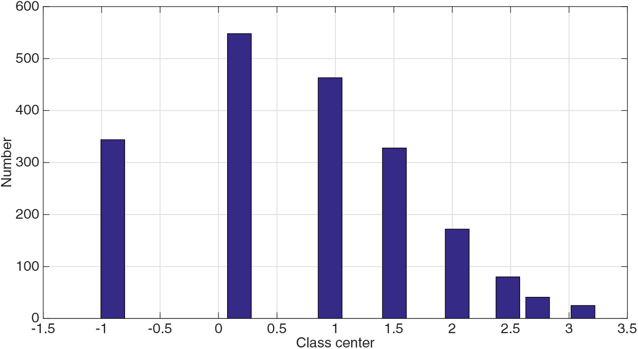
Figure 6: Sample size and corresponding class center distribution for each class in Case 2

Given that the initial value of the ESO is X^(0)=[0,0]T and the parameters of the ESO are l1 = 1 and l2 = 0.3. The initial value of the PPD estimation is φ^(0)=0.5, and the corresponding estimation algorithm parameters are η=1, μ=1. Similar to the Case 1, the proposed probability density evolution prediction and estimation method based on pattern motion is used to estimate the system output and predict the system pattern class, and the corresponding results are shown respectively in Figs. 7 and 8.

Figure 7: Comparison of system output estimation and actual system output in Case 2

Figure 8: Comparison of system pattern class estimation and actual system pattern class in Case 2

Based on the results from Figs. 7 and 8, it can be seen that, for systems with more complex nonlinear characteristics, the proposed method in this paper is still able to achieve good tracking estimation of the system output, and can accurately predict the class attribution of the system. From the comparison between the proposed method and traditional data-driven methods in Fig. 7, it can be observed that the proposed method provides more accurate estimation of the system, whereas the traditional method exhibits greater fluctuations. The reason is that, compared to Case 1, the overall distribution range of the system’s output in Case 2 is smaller. From the overall trend change of the system, the overall trend change of Case 2 is smaller than that of Case 1, which leads to a relatively larger impact of statistical characteristics on the system in Case 2. At this point, the pattern motion probability density evolution method proposed in this article has more advantages.

6  Conclusion

This article explores the issue of output prediction in non-Newtonian mechanical systems and proposes an analysis framework based on pattern motion probability density evolution. Within this framework, a data-driven pattern motion probability density prediction method is developed using PPD and probability density evolution theory, which only requires the current input-output data of the system and its statistical characteristics. In addition, based on the system’s output probability density prediction, unbiased estimation of the system’s output value is achieved through minimum variance estimation. Finally, this article combines an ESO to design a corresponding PPD estimation algorithm. The effectiveness of the proposed method is verified through theoretical analysis and numerical simulation.

From the construction of pattern motion probability density evolution prediction method, it can be inferred that this method is an analysis approach that utilizes statistical variables. This implies that the applicability of this method is mainly restricted to systems governed by statistical laws, and when the statistical properties of the system are stronger compared to other dynamic characteristics, this method is more effective compared to general nonlinear analysis methods. In addition, the construction of pattern motion variables requires the prior construction of system motion subspaces and pattern category scale spaces, which require the collection of sufficient historical data and analysis. In fact, the larger the historical dataset, the more complete the constructed motion subspace. Although pattern recognition analysis of historical data usually takes a long time, the advantage is that this process is offline and does not affect the real-time performance of the prediction algorithm. Furthermore, unlike methods that require selecting representative points to solve the generalized probability density evolution equation. In this paper, a data-driven form based on pseudo partial derivatives is constructed to directly solve the corresponding probability density evolution equation, greatly reducing the computational complexity.

Acknowledgement: The authors wish to express their appreciation to the reviewers and editors for their helpful suggestions which greatly improved the presentation of this paper.

Funding Statement: The authors received no specific funding for this study.

Author Contributions: The authors confirm contribution to the paper as follows: study conception and design: Cheng Han, Zhengguang Xu; draft manuscript preparation: Cheng Han. All authors reviewed the results and approved the final version of the manuscript.

Availability of Data and Materials: Not applicable. The experimental results in this article can be verified by computer simulation using the equations given in the example.

Conflicts of Interest: The authors declare that they have no conflicts of interest to report regarding the present study.

References

1. Qu, S. D. (1998). Pattern recognition approach to intelligent automation for complex industrial processes. Journal of University of Science and Technology Beijing, 20(4), 385–389. [Google Scholar]

2. Saridis, G. (1981). Application of pattern recognition methods to control systems. IEEE Transactions on Automatic Control, 26(3), 638–645. [Google Scholar]

3. Ye, N., Lu, Y. Z. (1988). Pattern recognition based state estimation-measurement aids with software. Chinese Journal of Scientific Instrument, 9(4), 368–374. [Google Scholar]

4. Zhou, X. J., Chai, T. Y. (2007). Pattern-based hybrid intelligent control for rotary kiln process. 2007 IEEE International Conference on Control Applications, pp. 31–35. Singapore. [Google Scholar]

5. Mendel, J. M., Zapalac, J. J. (1968). The application of techniques of artifical intelligence to control system design. Advances in Control Systems, 6, 1–94. [Google Scholar]

6. Fu, K. S. (1970). Learning control systems-review and outlook. IEEE Transactions on Automatic Control, 15(2), 210–221. [Google Scholar]

7. Xu, Z. G. (2001). Pattern Recognition Method of Intelligent Automation and Its Implementation in Engineering (Ph.D. Thesis). University of Science and Technology Beijing, China. [Google Scholar]

8. Xu, Z. G., Wang, M. S., Guo, L. L. (2019). State feedback asymptotic stability of a kind of complex production processes based on pattern moving. Control Theory and Applications, 36(2), 249–261. [Google Scholar]

9. Wang, M. S., Xu, Z. G., Guo, L. L. (2019). Stability and stabilization for a class of complex production processes via lmis. Optimal Control Applications and Methods, 40(3), 460–478. [Google Scholar]

10. Xu, Z. G., Wang, M. S., Guo, L. L. (2020). Relationship between clustering parameters and regulation performance of a class of production processes based on pattern moving. Control and Decision, 35(5), 1025–1038. [Google Scholar]

11. Xu, Z. G., Sun, C. P. (2012). Moving pattern measured by interval number for modeling and control. Control Theory and Applications, 29(9), 1115–1124. [Google Scholar]

12. Xu, Z. G., Sun, C. P. (2016). Multi-dimensional moving pattern prediction based on multi-dimensional interval T-S fuzzy model. Control and Decision, 31(9), 1569–1576. [Google Scholar]

13. Guo, L. L., Wang, Y. (2014). The application of cell mapping to dynamic modeling and control. Applied Mechanics and Material, 687, 661–664. [Google Scholar]

14. Li, X. Q., Xu, Z. G., Han, C., Li, N. (2022). Pattern-moving-based parameter identification of output error models with multi-threshold quantized observations. Computer Modeling in Engineering & Sciences, 130(3), 1807–1825. https://doi.org/10.32604/cmes.2022.017799 [Google Scholar] [CrossRef]

15. Li, X. Q., Xu, Z. G., Cui, J. R. (2021). Suboptimal adaptive tracking control for fir systems with binary-valued observations. Science China Information Sciences, 64(7), 172202. [Google Scholar]

16. Fokker, A. D. (1914). Die mittlere energie rotierender elektrischer dipole im strahlungsfeld. Annalen der Physik, 248(5), 810–820. [Google Scholar]

17. Kolmogoroff, A. (1931). Uber die analytischen methoden in der wahrscheinlichkeitsrechnung. Mathematische Annalen, 104, 415–458. [Google Scholar]

18. Fishman, G. (2013). Monte Carlo: Concepts, algorithms, and applications. New York: Springer Science and Business Media. [Google Scholar]

19. Hohenbichler, M., Rackwitz, R. (1988). Improvement of second-order reliability estimates by importance sampling. Journal of Engineering Mechanics, 114(12), 2195–2199. [Google Scholar]

20. Engelund, S., Rackwitz, R. (1993). A benchmark study on importance sampling techniques in structural reliability. Structural Safety, 12, 255–276. [Google Scholar]

21. Zhou, K., Tang, J. (2021). Uncertainty quantification of mode shape variation utilizing multi-level multi-response gaussian process. Journal of Vibration and Acoustics, 143, 011003. [Google Scholar]

22. Zhou, K., Tang, J. (2018). Uncertainty quantification in structural dynamic analysis using two-level gaussian processes and bayesian inference. Journal of Sound and Vibration, 412, 95–115. [Google Scholar]

23. Savoy, H., Hesse, F. (2019). Dimension reduction for integrating data series in bayesian inversion of geostatistical models. Stochastic Environmental Research and Risk Assessment, 33, 1327–1344. [Google Scholar]

24. Li, J., Chen, J. (2004). Probability density evolution method for dynamic response analysis of structures with uncertain parameters. Computational Mechanics, 34, 400–409. [Google Scholar]

25. Chen, J., Li, J. (2005). Dynamic response and reliability analysis of non-linear stochastic structures. Probabilistic Engineering Mechanics, 20, 33–44. [Google Scholar]

26. Wan, Z., Chen, J., Li, J. (2020). Probability density evolution analysis of stochastic seismic response of structures with dependent random parameters. Probabilistic Engineering Mechanics, 59, 103032. [Google Scholar]

27. Feng, D. C., Cao, X. Y., Beer, M. (2022). An enhanced PDEM-based framework for reliability analysis of structures considering multiple failure modes and limit states. Probabilistic Engineering Mechanics, 70, 103367. [Google Scholar]

28. Cao, X. Y., Feng, D. C., Beer, M. (2023). Consistent seismic hazard and fragility analysis considering combined capacity-demand uncertainties via probability density evolution method. Structural Safety, 103, 102330. [Google Scholar]

29. Chen, J. Y., Jia, Q. B., Xu, Q., Fan, S. L., Liu, P. F. (2021). The pdem-based time-varying dynamic reliability analysis method for a concrete dam subjected to earthquake. Structures, 33, 2964–2973. [Google Scholar]

30. Fan, W. L., Ang, A., Li, Z. L. (2017). Reliability assessment of deteriorating structures using bayesian updated probability density evolution method (PDEM). Structural Safety, 65, 60–73. [Google Scholar]

31. Hou, Z. S., Jin, S. T. (2013). Model free adaptive control: Theory and applications. Boca Raton: CRC Press. [Google Scholar]

32. Bu, X. H., Hou, Z. S., Yu, F. S. (2012). Robust model free adaptive control with measurement disturbance. IET Control Theory and Applications, 6, 1288–1296. [Google Scholar]

33. Hou, Z. S., Xiong, S. S. (2019). On model-free adaptive control and its stability analysis. IEEE Transactions on Automatic Control, 11(6), 4555–4569. [Google Scholar]

34. Chi, R. H., Hui, Y., Zhang, S. (2019). Discrete-time extended state observer-based model-free adaptive control via local dynamic linearization. IEEE Transactions on Industrial Electronics, 67(10), 8691–8701. [Google Scholar]

35. Chi, R. H., Hui, Y., Huang, B., Hou, Z. S. (2021). Active disturbance rejection control for nonaffined globally lipschitz nonlinear discrete-time systems. IEEE Transactions on Automatic Control, 66(12), 5955–5967. [Google Scholar]

36. Fang, H. Z., Tian, N., Wang, Y. B., Zhou, C. M., Haile, M. A. (2018). Nonlinear bayesian estimation: From kalman filtering to a broader horizon. IEEE/CAA Journal of Automatica Sinica, 5(2), 401–417. [Google Scholar]