A Subdivision-Based Combined Shape and Topology Optimization in Acoustics

1  Introduction

Computer aided engineering (CAE) is a numerical simulation process for analyzing product performance in a broad range of industries. Digital twin technology and industrial manufacturing both now heavily rely on CAE simulation. However, the present CAE depends on a preprocessing stage. That is, the geometric model generated by Computer aided geometric design (CAGD) software needs to be converted into one suitable for simulation. The conversion process for geometric data is the most time-consuming and error-prone manual intervention in CAE. Isogeometric analysis [1] directly applies geometric models from CAD software to the numerical computation of physical problems, eliminating the mesh regeneration process whilst maintaining geometrically accurate modelling, and therefore has received considerable attention from researchers [2–5] for application to acoustic problems.

In the current work, the boundary of analyzed domain can be represented by subdivision curves or surfaces. A number of CAD packages have recently added subdivision capabilities, including 3D Studio Max, Autodesk Fusion 360, SolidWorks and others. Subdivision curves/surfaces provide graceful isogeometric, bidirectional mapping between geometric and analytical models [6]. Subdivision uses a coarse mesh and a restricted process of duplicated refinement to describe geometric shapes [7–10]. Multiresolution subdivision surfaces have the following advantages: (1) Having the ability to represent topologically arbitrary geometries; (2) wavelet-like multiresolution representation of geometries; (3) Subdivision-friendly integration with CAD packages.

Geometric parameterization and its interaction with boundary element discretization play an important role in shape optimization [11–13]. When traditional BEM meshes are used for geometric parameterization, it leads to jaggedness in the optimized geometry, as is already known in the finite element method [14]. To address this challenge, geometries in shape optimization are often parameterized using B-splines or related techniques, such as NURBS [15,16] and subdivision surfaces [17–20]. In this research, we represent the domain geometries in terms of subdivision surfaces, which are spline extensions of arbitrarily connected meshes. Sound absorbing materials [21,22] reduce the noise intensity in the surrounding area by absorbing the acoustic waves radiated/scattered outwards from the structure, but full coverage of these materials applied to the surface of the structure will increase its weight and design cost. Adjusting the distribution of sound absorbing materials through topology optimization design [23–26] is important to achieve noise control.

The existing structural optimization designs generally focus on shape optimization or topology optimization of a single type, but the geometry and topology of structures in engineering problems need to be designed simultaneously to achieve better performance. Combined optimization methods have been developed and are generally divided into two categories, namely the level set method [27–29] and geometric interpolation modeling [30–33], to achieve shape and topology variations. The first category is the simultaneous change of structure shape and topology through the change of holes. Matsumoto et al. [34] applied it to calculate the shape and topology sensitivities for acoustic performance. The second category is represented by the deformable simplicial complex method, in which the shape optimization and topology optimization are in a state of continuous alternation, collectively referred to as a combined optimization iteration step. Jiang et al. [35] and Wang et al. [36] analyzed the optimization effects of different combined topology and shape iterative schemes by using two and three dimensional acoustic structures, respectively. They adopted the NURBS interpolation scheme to construct a channel for the connection between structural shape and surface material distribution.

The combined optimization can be operated through the method of moving asymptotes (MMA) [37,38] based on gradient solvers, in which the sensitivity information of the objective function is required. Finite difference method (FDM), direct differentiation method (DDM) [39,40] and adjoint variable method (AVM) [41,42] are the three main methods for shape and topological sensitivity analysis. Amongst them, AVM shows higher efficiency for solving the sensitivity of multiple design variables, and a more efficient AVM is applied in this research compared with that in our previous work [20]. For the geometric jagged oscillations that appear during shape optimization, smooth surfaces are obtained by mesh editing in the multi-resolution method. For density discontinuities that appear during topology optimization, the solid isotropic material penalty method (SIMP) [43,44] is used to interpolate the materials into continuous variables of density. This work has made the following contributions: (1) To improve the calculation efficiency, the calculation formula of discrete adjoint variables of shape sensitivity is derived, and the efficient calculation of topology and shape sensitivity is realized. (2) Compared with geometric shape optimization based on NURBS and other geometric shapes, shape optimization based on subdivision surface interpolation has the flexibility of shape control, and can maintain the smoothness of the surface after inverse processing.

This paper is devoted to developing a combined optimization approach with subdivision surface boundary elements for acoustic problems. The rest of the sections are structured in the following manner: Section 2 introduces the subdivision rules for Catmull-Clark subdivision curves/surfaces and the boundary element method with impedance boundary conditions in acoustics. Sensitivity analysis via AVM with subdivision surface control points and the density of sound absorbing material is presented in Section 3. Section 4 describes the topology optimization, shape optimization, and combined optimization process. Section 5 contains numerical tests to validate the presented combined optimization method. Finally, Section 6 elaborates the conclusions of this work.

2  Subdivision Surfaces BEM for the Acoustic Domain

2.1 Catmull-Clark Subdivision Surfaces

In the context of isogeometric analysis, the subdivision surface basis function enables the representation of the identical spline surface using control meshes of different resolutions [45]. The particular division guidelines employed in this study are obtained from cubic B-splines.To achieve smooth surfaces for curves/surfaces, we employ the subdivision principle introduced by Catmull et al. [46]. This technique ensures that even unstructured meshes with irregular vertices (i.e., vertices having a varying number of adjacent edges other than 4) yield smooth surfaces. In Fig. 1, the initial mesh and convergence surface for the Catmull-Clark subdivision rule are depicted in both two and three dimensions.

Figure 1: The Catmull-Clark subdivision curve and surface

Each subdivision operation generate a new vertex vx by moving the original mesh node, and new vertices ex and fx are inserted respectively at the midpoint of edges and the center of the element. All newly inserted nodes make up a new mesh level. The control vertex coordinates for a fine mesh at level k+1 are determined by the vertex coordinates of the coarse mesh at level k

xk+1=Sxk,(1)

where xk and xk+1 denote two vectors that store the vertex coordinates of meshes at the coarser level and those at the refined level, respectively. Matrix S is the global subdivision matrix with size [Nv+Ne+Nf,Nv], where Nv represents the total number of vertices. The subdivision matrix S includes standard weights for inserting junctions in regular mesh vertices. The matrix components corresponding to the vertices of the irregular region can be obtained through a particular subdivision method, which can be referred to [47]. A linear mapping can be interpreted as the continuous subdivision refinement of the control mesh:

x0→Sx1→Sx2→S⋯→Sxk−1→Sxk,(2)

The number of vertex coordinates xk increases as k increases, and the size of subdivision matrix S increases accordingly. Regardless of the arbitrary level, all control meshes converge to the same surface.

Multiresolution analysis brings editability to different levels of the subdivision surface [48–50]. In shape optimization, a well-performing geometric configuration can be obtained by alternately refining and coarsening the control mesh. Establish the relationship between the control points at levels k+1 and k through coarsening matrix R, as follows:

xk=Rxk+1.(3)

where R=(STS)−1ST is the coarsening matrix. Similar to subdivision refinement, to obtain a coarser representation of geometry, coarse matrices can be applied sequentially as follows:

xk→Rxk−1→Rxk−2→R⋯→Rx1→Rx0.(4)

The coordinates of the vertices represented by one step of refinement, followed by one step of coarsening, do not change, so the relationship between the subdivision matrix and the inverse matrix is RS=I. Under the subdivision surface, the hierarchy of control meshes is naturally used for multiresolution geometry decomposition [51,52]. For this purpose, the size of the geometric area influenced by each vertex is determined by the resolution of the control mesh, with editing coarser layers producing large-scale changes and editing thinner layers producing small-scale changes. Local subdivision refinement can be applied to the surface of the corresponding being edited.

2.2 Subdivision Surface BEM with Impedance Boundary Condition

This study considers the differential equation that governs the harmonic acoustic wave:

∇2p(x)+k2p(x)=0,∀x∈Ω,(5)

where ∇2 is the Laplace operator, p denotes the sound pressure, k=ω/c denotes the wave number, ω is the angular frequency, and c is the wave speed in the acoustic medium Ω.

For the acoustic boundary element method [53,54], the boundary integral expression and its outward normal derivative formulation of the Helmholtz equation are as follows:

c(x)p(x)=∫SG(x,y)q(y)dS(y)−∫SF(x,y)p(y)dS(y)+pinc(x),(6)

c(x)q(x)=∫SG1(x,y)q(y)dS(y)−∫SF1(x,y)p(y)dS(y)+∂pinc(x)∂n(x),(7)

where x and y are the field point and the source point, respectively. S is the boundary of the Ω. For the 3D problem the Green’s functions [55,56] are given as

G(x,y)=eikr4πr,(8)

F(x,y)=−eikr4πr2(1−ikr)∂r∂n(y),(9)

G1(x,y)=−eikr4πr2(1−ikr)∂r∂n(x),(10)

F1(x,y)=eikr4πr3[(3−3ikr−k2r2)∂r∂n(x)∂r∂n(y)+(1−ikr)nl(x)nl(y)],(11)

where r=∣x−y∣ is the distance from the source point to the field point, and nl is the Cartesian component of n(x) or n(y). The admittance boundary condition is expressed as

q(y)=ikβ(y)p(y),(12)

where β(y) represents the normalized surface admittance at point y. Note that when β(y)=0, the impedance boundary degenerates into a rigid boundary, i.e., the surface shows total reflection and does not absorb any sound waves.

After introducing the impedance boundary condition, the sound pressure and flux on the surface boundary can be discretized as follows:

p(ξ,η)=∑a=1NaBa(ξ,η)pa,q(ξ,η)=ikβ∑a=1NaBa(ξ,η)pa,(13)

where pa is the coefficients of sound pressure, Ba denotes the bicubic B-spline basis function [47] and Na represents the total number of basis functions. Substituting the above equation into Eqs. (6) and (7) after discretizing the boundary into Ne elements yields:

12∑a=1NaBa(ξ,η)pa=∑e=1Ne∑a=1Naikβ[∫SeG(x,y)Ba(ξ,η)dSe]pa−∑e=1Ne∑a=1Na[∫SeF(x,y)Ba(ξ,η)dSe]pa+pinc(x),(14)

and

12ikβ∑a=1NaBa(ξ,η)pa=∑e=1Ne∑a=1Naikβ[∫SeG1(x,y)Ba(ξ,η)dSe]pa−∑e=1Ne∑a=1Na[∫SeF1(x,y)Ba(ξ,η)dSe]pa+∂pinc(x)∂n(x),(15)

where c(x)=1/2 on the smooth surface boundary. Using the Burton-Miller method [57–59] to linearly combine Eqs. (14) and (15), then expressed in matrix form as follows:

[H−G]p=pinc,(16)

where H and G represent the matrices formed by the integrals in Eqs. (14) and (15), respectively. p denotes the vector of sound pressure, and pinc are the vectors of incident sound pressure and flux.

Once the sound pressure at the boundary is acquired, it can be represented in matrix form to express the sound pressure at various points within a given domain:

pf=[Gf−Hf]p+pinf,(17)

where the subscript f denotes the computation point is inside the acoustic domain.

3  Sensitivity Analysis through Subdivision Surface BEM

3.1 Topology Sensitivity Analysis

In this research, topology optimization is performed for the distribution of acoustic absorbing materials with discrete values of 0 or 1 on the structure surface. AVM is adopted for the topology sensitivity analysis. The discrete values are transformed into continuous ones using the SIMP method. The design parameter for the optimization process is set to the artificial density ρe of element e. The equation of admittance by the SIMP method can be expressed as

βe=β0ρeε,(18)

where β0 represents the normalized surface acoustic admittance, ε denotes the penalization coefficient determining the intermediate density tending to zero or one. The determination of the penalty coefficient is detailed in [60]. ε is set to 3 in the present analysis.

The goal of this study is to establish a relationship between the objective function Π(pf) and the sound pressure in acoustic optimization. In accordance with Eqs. (16) and (17), the reconstructed objective function Π can be rewritten as

Π=Π(pf)+ℜ{λ1T[(H−G)p−pinc]+λ2T[pf+(Hf−Gf)p−pinf]},(19)

where Π is a real valued function, and ℜ denotes the process of extracting the real component of the complex number.

λ1T and λ2T represent the transposed adjoint vectors of the boundary of the structure and the points in the field, respectively. By differentiating the above equation with regard to the design variable ρe yields the following equation:

∂Π∂ρe=∂Π(pf)∂ρe+ℜ{λ1T[(H−G)∂p∂ρe−∂G∂ρep]}+ℜ{λ2T[∂pf∂ρe+(Hf−Gf)∂p∂ρe−∂Gf∂ρep]},(20)

The formulation of the derivative of the objective function Π(pf) can also be expressed as

∂Π(pf)∂ρe=ℜ(v1+v2T∂p∂ρe+v3T∂pf∂ρe),(21)

The values of v1, v2T, and v3T in the objective function expression are determined by the specific expression of Π(pf). Eq. (20) can be further written as

∂Π∂ρe=−ℜ(λ1T∂G∂ρep+λ2T∂Gf∂ρep+v1)+ℜ[(λ2T+v3T)∂pf∂ρe]+ℜ{[λ1T(H−G)+λ2T(Hf−Gf)+v2T]∂p∂ρe},(22)

where the adjoint vectors λ1T and λ2T can be arbitrarily selected as long as they meet the following equation:

{λ2T+v3T=0λ1T(H−G)+λ2T(Hf−Gf)+v2T=0(23)

For all topology design variables, the system of adjoint Eq. (23) should be solved only once to obtain adjoint vectors λ1 and λ2. Hence, the use of AVM can greatly enhance the computational effectiveness of topology sensitivity analysis, which holds immense importance for topology optimization.

3.2 Shape Sensitivity Analysis

In this research, the geometry configuration of the structure is changed by modifying the location of the control points. We use AVM to perform shape sensitivity analysis and set the control points on subdivision surfaces as shape design parameters. Eqs. (6) and (7) can be derived as follows:

c(x)∂p(x)∂χe=∫S[∂G(x,y)∂χeq(y)−∂F(x,y)∂χep(y)]dS(y)+∫S[G(x,y)∂q(y)∂χe−F(x,y)∂p(y)∂χe]dS(y)+∫S[G(x,y)q(y)−F(x,y)p(y)]d∂S(y)∂χe+∂pinc(x)∂χe,(24)

and

c(x)∂q(x)∂χe=∫S[∂G1(x,y)∂χeq(y)−∂F1(x,y)∂χep(y)]dS(y)+∫S[G1(x,y)∂q(y)∂χe−F1(x,y)∂p(y)∂χe(y)]dS(y)+∫S[G1(x,y)q(y)−F1(x,y)p(y)]d∂S(y)∂χe+∂2pinc(x)∂n(x)∂χe,(25)

where χe denotes the coordinates in x, y, and z directions of control points, and ∂()∂χe represents the sensitivity values at the control points.

Afterwards, Eqs. (24) and (25) are rewritten as

12∑a=1NaBa(ξ,η)∂pa∂χe=∑e=1Ne∑a=1Napa∫Se[ikβe∂G(x,y)∂χe−∂F(x,y)∂χe]Ba(ξ,η)dSe+∑e=1Ne∑a=1Na∂pa∂χe∫Se[ikβeG(x,y)−F(x,y)]Ba(ξ,η)dSe+∑e=1Ne∑a=1Napa∫Se[ikβeG(x,y)−F(x,y)]Ba(ξ,η)d∂S(y)∂χe+∂pinc(x)∂χe,(26)

and

12∑a=1NaikβiBa(ξ,η)∂pa∂χe=∑e=1Ne∑a=1Napa∫Se[ikβe∂G1(x,y)∂χe−∂F1(x,y)∂χe]Ba(ξ,η)dSe+∑e=1Ne∑a=1Na∂pa∂χe∫Se[ikβeG1(x,y)−F1(x,y)]Ba(ξ,η)dSe+∑e=1Ne∑a=1Napa∫Se[ikβeG1(x,y)−F1(x,y)]Ba(ξ,η)d∂S(y)∂χe+∂2pinc(x)∂n(x)∂χe.(27)

Similarly, combining Eqs. (26) and (27) using the Burton-Miller method yields the system of equations for sensitivity as follows:

(H−G)∂p∂χe=(∂G∂χe−∂H∂χe)p+pinc∂χe,(28)

where matrices H and G have been computed in Eq. (16), and ∂H∂χe and ∂G∂χe are their derivative matrices. Similarly, the matrix form of the points in the domain is obtained by

∂pf∂χe=(∂Gf∂χe−∂Hf∂χe)p−(Hf−Gf)∂p∂χe+∂pinf∂χe,(29)

In shape optimization design, the boundary shape of a structure often needs to be described by functions that take multiple design variables as parameters. To improve the efficiency of acoustic sensitivity analysis of multiple design variables with increased practical significance, the discrete AVM [56] is introduced next. The acoustic pressure sensitivity calculation matrix for the boundary point can be written as

∂p∂χe=(H−G)−1[(∂G∂χe−∂H∂χe)p+∂pinc∂χe],(30)

Substituting the above expression into Eq. (29) gives:

∂pf∂χe=−(Hf−Gf)(H−G)−1[(∂G∂χe−∂H∂χe)p+∂pinc∂χe]+(∂G∂χe−∂Hf∂χe)p+∂pinf∂χe,(31)

where the inverse operation of matrix (H−G) requires considerable time, so the accompanying equation is defined as follows:

(H−G)TA=(Hf−Gf)T,(32)

where AT=(Hf−Gf)(H−G)−1, which is integrated into Eq. (31) to obtain the sound pressure sensitivity of the domain point, as shown as follows:

∂pf∂χe=−AT[(∂G∂χe−∂H∂χe)p+∂pinc∂χe]+(∂Gf∂χe−∂Hf∂χe)p+∂pinf∂χe,(33)

where adjoint matrix A is independent of shape design parameters χe. For multiple design parameter problems, its only needs to be solved once. This paper pushes further on previous research work [20] to improve the efficiency of the discrete AVM for computing shape sensitivity.

4  Combined Optimization Based on Subdivision Surface BEM

4.1 Topology Optimization Model

After the topology sensitivity analysis, the objective function is defined as the sound pressure level of the observer points in the acoustic domain, and the initial state is set as the structure surface fully attached to the sound absorbing material. The topology optimization model is given as follows:

{min:Π=20log10⁡((pfHpf)2.0×10−5),s.t.:∑e=1Neρeve−V0e∑e=1Neve≤0,Bound:0≤ρmin≤ρe≤1,e=1,…,Ne,Iter.:|Πj+1−ΠjΠj|<τ,(34)

where Π is the objective function, ()H denotes the symbol for the conjugate transpose. The optimized constraint function is set to the volume constraint of the sound absorbing material distribution; ve is the volume of each piece of material, which corresponds to the area of the subdivision surface integral element; the volume constraint score is V0e=0.5. The corresponding material on each subdivision surface element is a topology design variable ρe. To avoid the problem of singular values, the lower limit of the topology design variable is ρmin=0.001. The number of topology design variables is equal to the number of subdivision surface integral elements for the structure surface.

According to Eq. (21), the objective function [36] here is the sound pressure level of the test points, and v1, v2T, and v3T can be set as follows:

{v1=0,v2T=0,v3T=10ln⁡101pfHpf⋅2pfH.(35)

After the sound field analysis and solving of adjoint vectors λ1 and λ2, the objective function sensitivity can be obtained in the optimization process.

4.2 Shape Optimization Model

After the shape sensitivity analysis, using the same objective function as in topology optimization, a shape optimization model is established with the control point coordinates as design variables. The shape optimization model is given as follows:

{minΠ=20log10((pfHpf)2.0×10−5),s.t.V(χe)−V0⩽0,Boundχemin⩽χe⩽χemax,Iter∣Πj+1−Πj∣Πj<τ,(36)

where V0 represents the initial volume of the structure, and V(χe) denotes the volume after the changes of control points. For each design variable, χemax and χemin are set as the top and lower bounds of its values. In this paper, a local boundary is chosen as the shape optimization region, and a single direction of control point coordinates is chosen to facilitate shape changes.

For shape optimization, the structure’s volume V can be calculated by integrating over the points x and their external normal vectors n on the subdivision surface. The volume function and its sensitivity can be expressed as follows:

V=∫ΩdΩ=13∑e=1Ne∫01∫01x⋅nJe(ξ,η)dξdη.(37)

∂V∂χe=13∑e=1Ne∫01∫01[∂x∂χe⋅nJe(ξ,η)+x⋅∂n∂χeJe(ξ,η)+x⋅n∂Je(ξ,η)∂χe]dξdη,(38)

4.3 Iteration Schemes of the Combined Optimization

Traditional optimization methods tend to focus on one type of optimization of the structure, such as topology or shape optimization alone. In this subsection, the combined optimization based on subdivision surface BEM is implemented to achieve efficient noise reduction. Fig. 2 displays the flowchart of the combined optimization approach for the 3D structure. The process is primarily divided into seven steps, which are as follows:

1.    The subdivision surface model of the initial structure is input, and the appropriate optimization levels are selected according to the refinement of initial model and topology and shape design needs.

2.    The definition of the topology optimization model is based on the refinement surface, and sound field and topology sensitivity analyses. The objective function, the constraint function and its sensitivity value are calculated.

3.    The MMA algorithm is used to update the topology design variables, and SIMP is carried out to filter intermediate densities.

4.    The shape optimization model under the impedance boundary is defined according to the refinement surface, and sound field and shape sensitivity analyses. The objective function, the constraint function and its sensitivity value are calculated.

5.    The MMA algorithm is used to update the shape design variables, and the multiresolution approach is adopted to eliminate jagged geometry.

6.    Combined scheme is selected for optimization iteration. Fig. 2 shows three different combination schemes. In combined A, an iterative step contains one-step topology optimization and one-step shape optimization. Combined B contains complete topology optimization and one-step shape optimization in an iterative step. Combined C contains one-step topology optimization and complete shape optimization in an iterative step.

7.    The geometric configuration and sound absorption material distribution of the structure are output after combined optimization.

Figure 2: The combined optimization process

5  Numerical Examples

The applicability of the proposed approach is verified by numerical examples, and its potential in engineering applications is demonstrated by a muffler pipe example. Here, all the examples are solved under the boundary condition of sound absorption and external acoustics, and the convergence coefficient τ is set to 10−4.

5.1 Cylinder Model

A sensitivity analysis and the combined optimization approach are calculated for a simple cylinder model. Fig. 3 shows the physical optimization model. The blue point is selected as the observation point with coordinates (0,0,3). Shape design variables include 12 points that are colored red. The cylinder’s length is 6 m, and the hemispherical’s radius is 1 m. Fig. 4 shows the multilevel subdivision meshes for the cylinder model. The number of elements and vertices of the initial mesh is 304 and 306, and the Catmull-Clark Subdivision surface of the quadrilateral element is used to obtain the subdivision meshes of different levels. The number of elements and vertices corresponding to the first subdivision level is 1216 and 1218, and the mesh of second subdivision level is selected for the objective function and sensitivity analysis.

Figure 3: Physical problem of a cylinder model

Figure 4: Multilevel subdivision meshes for cylinder model

5.1.1 Sensitivity Analysis

Firstly, the cylinder model undergoes sensitivity analysis and verification are carried out for shape and topology design variables. Fig. 5 shows the shape sensitivity of sound pressure corresponding to the methods of FDM, DDM and AVM, and the excitation frequency is 100 Hz. The sensitivity values obtained under different solution methods are consistent. Fig. 6 compares the sensitivity calculation times of DDM and AVM with the increase in design variables. AVM becomes more efficient compared to DDM as the quantity of design variables increases. At the same time, the efficiency benefits of AVM are more obvious than those of DDM. Fig. 7 shows the sound pressure sensitivity distributions with all topology design parameters corresponding to the methods of FDM and AVM both the real and imaginary parts. The sensitivity value has a certain range of fluctuations (−0.001,0.001) on the side near the plane wave, and the value is close to 0 on the divergence sides.

Figure 5: The sound pressure sensitivity with the shape design variables

Figure 6: Comparison of computing times for shape sensitivity via DDM and AVM

Figure 7: The sound pressure sensitivity with the topology design variables

5.1.2 Optimization Design

Next, utilizing the accurate sensitivity data, the combined optimization design of cylinder structure with the objective of reducing the sound pressure level at the observation point is carried out. Fig. 8 presents the iteration processes of shape optimization, topology optimization and combined scheme B. Compared with the direct adhesion of the sound absorbing material on the structure surface, the reduction in the objective function caused by the change in shape is less than that by topology optimization at the corresponding test point. Given that the sound absorbing material is initially set as full coverage, the objective function increases in the second iteration step, and then gradually decreases until convergence in reasonable optimization calculations. In the process of combined scheme B, the first complete topology optimization will cause the objective function to converge to a certain value, and the addition of complete topology optimization to each step loop will make the objective function of the second step decrease greatly. Fig. 9 shows the optimal solution corresponding to different optimization methods. The material distribution in topology optimization is basically the same as that in combined optimization, but obvious differences occur in places where the shape changes greatly.

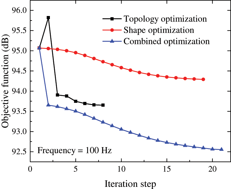
Figure 8: The iteration history of different optimization methods at 100 Hz

Figure 9: The optimal solution corresponding to different optimization methods at 100 Hz

The sound pressure distributions on the surface of the structure before and after optimization are shown in Fig. 10. The real, imaginary and amplitude parts of the sound pressure are included in turn. The place where large changes happen before and after optimization is in the area where the shape design parameters are located. As the structure is axisymmetric, the final optimization result is also symmetrically distributed.

Figure 10: Comparison of sound pressure on cylinder surfaces before and after optimization at 100 Hz

Table 1 shows the objective function values under different optimization schemes. The comparison of the optimization results indicates that the combined better optimization results than the single optimization. Fig. 11 shows the calculation times of different optimization schemes, from the calculation times of the single shape or topology optimization are less than those of combined optimization schemes. The calculation times of different combined schemes vary with respect to frequency, of which combined A scheme has a shorter CPU time than the other combination schemes at most frequencies. Thus, the subsequent parameter investigation adopts combined A scheme.

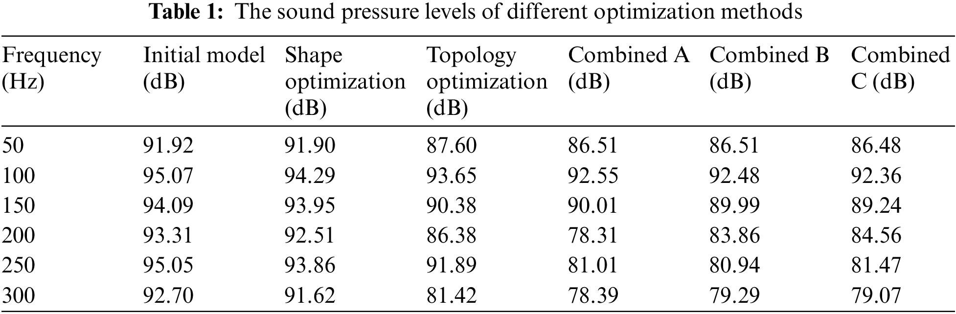
Figure 11: Comparison of the CPU time for different optimization methods

Figs. 12 and 13 show the optimization results for different combined schemes at 50 and 150 Hz. The distribution of optimization results is basically the same under different combination schemes, although differences are observed in few localised areas. The optimized shape and the distribution of sound absorbing materials are more dispersed at 150 Hz, which is due to the shorter wavelength at higher frequency.

Figure 12: Optimization results of different combined schemes at 50 Hz

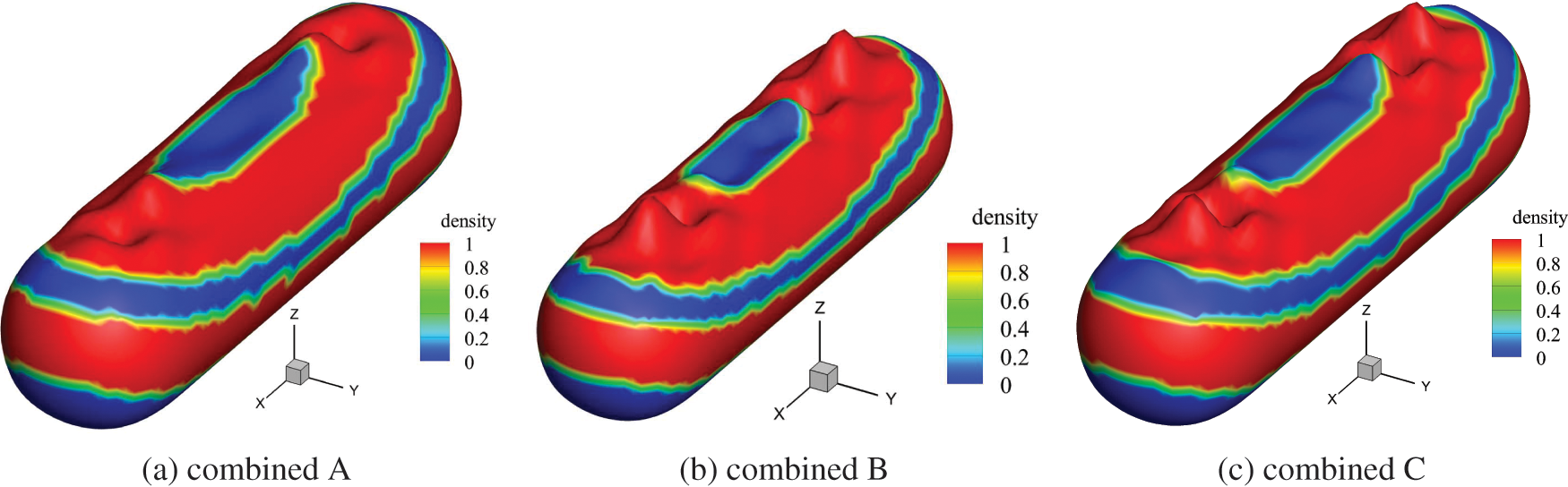
Figure 13: Optimization results of different combined schemes at 150 Hz

Lastly, the influence of different observation points on the optimization results is examined. Ten test points are selected in the y0z plane with radius 3 shown in Fig. 14, and the average sound pressure level is set as the objective function. The optimized result is shown in Fig. 15. The initial Πinit is 92.64 dB and the optimized Πopt under combined optimization is 92.43 dB at 50 Hz. The initial Πinit is 91.87 dB and the optimized Πopt of combined optimization is 90.19 dB at 150 Hz. The optimization effect is inconsiderably significant compared with that for a single test point. The sound pressure level optimized well at one point, but may perform worse at other points, so the average sound pressure level is more meaningful for engineering. Fig. 16 shows the comparison of sound fields before and after combined optimization A. From left to right, the initial sound field, the optimized sound field where 1 test point is located and the optimized sound field where 10 test points are located are presented. The distribution of the sound field suggests that the sound pressure level changes greatly in the case of single-point optimization, and the average sound pressure level changes minimally in the case of multi-point optimization.

Figure 14: Physical problem of a cylinder model with ten test points

Figure 15: Optimization results at different frequencies with 10 test point

Figure 16: Comparison of the sound field before and after optimization

5.2 Muffler Pipe Model

For optimal design of a muffler pipe model [20], the combined optimization approach is taken into consideration in the following subsection. Firstly, the boundary condition is set to be a rigid boundary on the outer surface and a sound absorption boundary on the inner surface. The region for structural optimization is the inner surface of the muffler pipe, the optimized shape control points are the 38 red coordinate points shown in Fig. 17, and the optimized topology design variables are the subdivision surface elements in the inner surface adhesion of the sound absorbing material (where the red portion represents the attachment of the sound absorbing substance, while the blue portion represents the non-adhesive sound absorbing material). Under the action of the plane wave traveling along the x-axis, the observation point is set at the central position of the outlet plane of the pipeline (−3,1.5,1.5). The initial model contains 736 elements and 736 nodes, and the second level of subdivision mesh is used for sound field and optimization.

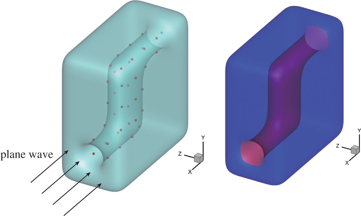
Figure 17: Physical problem of a muffler pipe model

Fig. 18 shows the iterative history of the muffler pipe model at 60 and 120 Hz frequencies in different combined optimization, from which the objective function of topology optimization at 60 Hz presents signs of increase. The inner surface of the structure is initially fully covered with sound absorbing materials. The final coefficient of the topology iterative scheme setting is less than 0.5 of the initial value, which makes the final optimization result greater than the initial value. However, the objective function of the combined optimization at different frequencies is reduced. Figs. 19 and 20 show that the optimization results for different optimization schemes are in the order of topology, shape, combined A, combined B and combined C. From the final optimized distribution, local differences exist in the distribution of shape and inner surface materials.

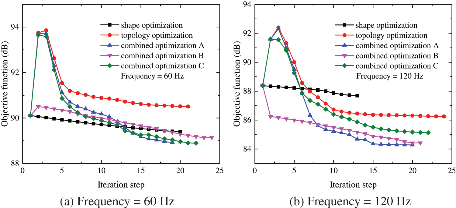
Figure 18: Iteration history at different frequencies

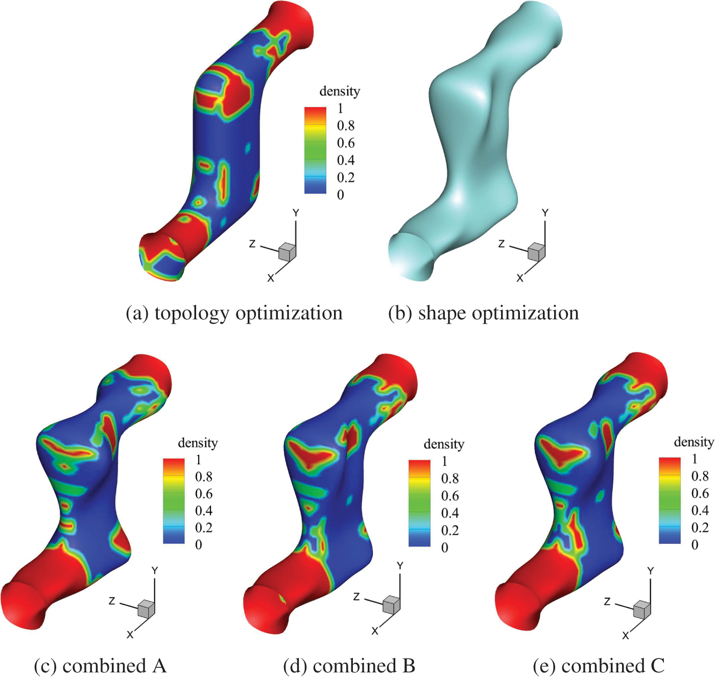
Figure 19: Optimization results of different combination schemes at 60 Hz

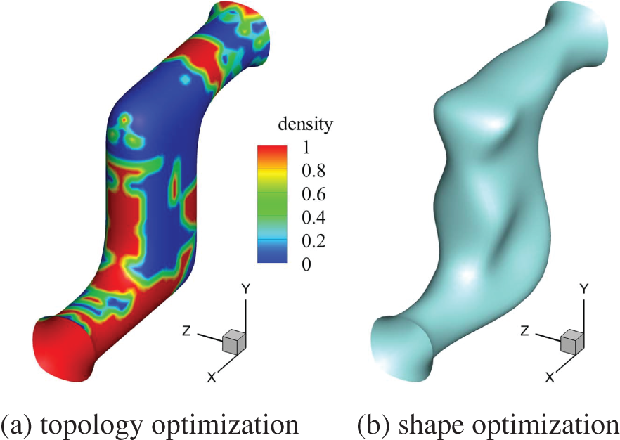
Figure 20: Optimization results of different combination schemes at 120 Hz

Next, the influence of the initial value of sound absorption coefficient on the optimization result is investigated. Fig. 21 shows the optimal distributions corresponding to the initial values 0.6 and 0.8 with different optimization approaches. Different initial values correspond to different initial objective functions: Πinit is 90.695 dB with the initial value of 0.6, Πinit is 88.801 dB with the initial value of 0.8, and Πinit is 88.376 dB with the initial value of 1.0. The final objective functions of combined optimization corresponding to the three initial values are 84.467, 84.295, and 84.425 dB, respectively. The optimization results are basically consistent with only slight differences in some elements. Thus, the final optimization result is not sensitive to the initial sound absorption coefficient.

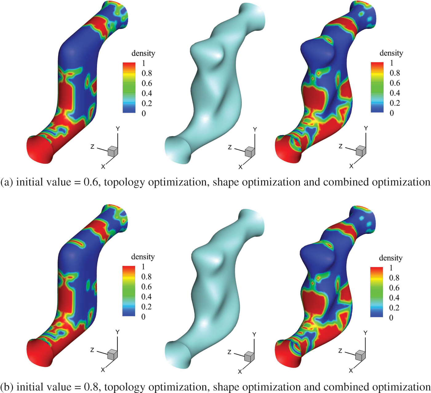
Figure 21: Optimization results with different initial values 0.6 and 0.8

Lastly, the sound fields before and after the combined optimization are compared. Fig. 22 shows the comparison of sound fields before and after optimization corresponding to different initial values. The external sound fields of the structure are basically the same, but the internal sound fields have much differences. When the sound absorption coefficient is low, the overall internal sound pressure level is larger owing to the stronger reflection effect of the sound wave, and the optimization effect at the outlet is more significant.

Figure 22: Comparison of the sound field before and after optimization

6  Conclusion

A combined optimization method for acoustic boundary elements of subdivision surfaces is presented. Based on impedance boundary conditions, the subdivision surface modeling is used as a medium to establish a link between the structural geometry and the distribution of the sound absorbing material. Alternating changes in structural shape and material distribution in the optimization iteration step are achieved. The control points of the fine geometry are selected as shape design variables, and the material density on each surface element is selected as the topology design variable for combined optimization, which shortens the calculation time for shape and topology sensitivity under multiple design variables by using AVM. Compared with geometric shape optimization based on NURBS and other geometric shapes, shape optimization based on subdivision surface interpolation has the flexibility of shape control, and can maintain the smoothness of the surface after inverse processing. Numerical examples show that the combined optimization provides better objective function reduction than single type of shape or topology optimization. The computation time for combined A is less than those for the other two schemes, and the optimization results obtained are similar to those of other combinatorial schemes. The impacts of the pertinent parameters and conditions are investigated, and the potential of the developed combinatorial optimization algorithm for application to engineering problems is verified.

In future work, we aim to study local adaptive subdivision surface methods and fast algorithms to larger-scale practical engineering problems. In consideration of the effects of structural vibrations, coupled finite element and boundary element analyses are necessary.

Acknowledgement: The authors acknowledge the financially support from the National Natural Science Foundation of China. We also appreciate the CAS Key Laboratory of Mechanical Behavior and Design of Materials for providing the high performance computing resources for this study.

Funding Statement: This work was financially supported by the National Natural Science Foundation of China (NSFC) under Grant Nos. 12172350, 11772322 and 11702238.

Author Contributions: The authors confirm contribution to the paper as follows: study conception and design: Chuang Lu, Leilei Chen, Haibo Chen; data collection: Chuang Lu, Jinling Luo; analysis and interpretation of results: Leilei Chen, Jinling Luo, Haibo Chen; draft manuscript preparation: Chuang Lu, Haibo Chen. All authors reviewed the results and approved the final version of the manuscript.

Availability of Data and Materials: Data will be made available on request.

Conflicts of Interest: The authors declare that they have no conflicts of interest to report regarding the present study.

References

1. Hughes, T. J., Cottrell, J., Bazilevs, Y. (2005). Isogeometric analysis: CAD, finite elements, NURBS, exact geometry and mesh refinement. Computer Methods in Applied Mechanics and Engineering, 194(39–41), 4135–4195. [Google Scholar]

2. Simpson, R. N., Scott, M. A., Taus, M., Thomas, D. C., Lian, H. (2014). Acoustic isogeometric boundary element analysis. Computer Methods in Applied Mechanics and Engineering, 269(139), 265–290. [Google Scholar]

3. Inci, E. O., Coox, L., Atak, O., Deckers, E., Desmet, W. (2020). Applications of an isogeometric indirect boundary element method and the importance of accurate geometrical representation in acoustic problems. Engineering Analysis with Boundary Elements, 110(39), 124–136. [Google Scholar]

4. Venås, J. V., Kvamsdal, T. (2020). Isogeometric boundary element method for acoustic scattering by a submarine. Computer Methods in Applied Mechanics and Engineering, 359, 112670. [Google Scholar]

5. Shaaban, A. M., Anitescu, C., Atroshchenko, E., Rabczuk, T. (2023). Isogeometric indirect BEM solution based on virtual continuous sources placed directly on the boundary of 2D Helmholtz acoustic problems. Engineering Analysis with Boundary Elements, 148(39), 243–255. [Google Scholar]

6. Cirak, F., Ortiz, M., Schröder, P. (2000). Subdivision surfaces: A new paradigm for thin-shell finite-element analysis. International Journal for Numerical Methods in Engineering, 47(12), 2039–2072. [Google Scholar]

7. Ma, W. (2005). Subdivision surfaces for CAD—An overview. Computer Aided Design, 37(7), 693–709. [Google Scholar]

8. Zhuang, C., Zhang, J., Qin, X., Zhou, F., Li, G. (2012). Integration of subdivision method into boundary element analysis. International Journal of Computational Methods, 9(1), 1240019. [Google Scholar]

9. Alderson, T., Mahdavi-Amiri, A., Samavati, F. (2021). RIAS: Repeated invertible averaging for surface multiresolution of arbitrary degree. IEEE Transactions on Visualization and Computer Graphics, 27(8), 3546–3557. [Google Scholar] [PubMed]

10. Kang, H., Hu, W., Yong, Z., Li, X. (2022). Isogeometric analysis based on modified loop subdivision surface with improved convergence rates. Computer Methods in Applied Mechanics and Engineering, 398(39–41), 115258. [Google Scholar]

11. Wall, W. A., Frenzel, M. A., Cyron, C. (2008). Isogeometric structural shape optimization. Computer Methods in Applied Mechanics and Engineering, 197(33–40), 2976–2988. [Google Scholar]

12. Kiendl, J., Schmidt, R., Wüchner, R., Bletzinger, K. U. (2014). Isogeometric shape optimization of shells using semi-analytical sensitivity analysis and sensitivity weighting. Computer Methods in Applied Mechanics and Engineering, 274, 148–167. [Google Scholar]

13. Lian, H., Kerfriden, P., Bordas, S. P. A. (2017). Shape optimization directly from CAD: An isogeometric boundary element approach using T-splines. Computer Methods in Applied Mechanics and Engineering, 317(4), 1–41. [Google Scholar]

14. Braibant, V., Fleury, C. (1984). Shape optimal design using B-spline. Computer Methods in Applied Mechanics and Engineering, 44(3), 247–267. [Google Scholar]

15. Liu, C., Chen, L., Zhao, W., Chen, H. (2017). Shape optimization of sound barrier using an isogeometric fast multipole boundary element method in two dimensions. Engineering Analysis with Boundary Elements, 85, 142–157. [Google Scholar]

16. Lüdeker, J. K., Sigmund, O., Kriegesmann, B. (2020). Inverse homogenization using isogeometric shape optimization. Computer Methods in Applied Mechanics and Engineering, 368, 113170. [Google Scholar]

17. Bandara, K., Cirak, F., Of, G., Steinbach, O., Zapletal, J. (2015). Boundary element based multiresolution shape optimisation in electrostatics. Journal of Computational Physics, 297, 584–598. [Google Scholar]

18. Bandara, K., Cirak, F. (2018). Isogeometric shape optimisation of shell structures using multiresolution subdivision surfaces. Computer Aided Design, 95, 62–71. [Google Scholar]

19. Zapletal, J., Bouchala, J. (2019). Shape optimization and subdivision surface based approach to solving 3D Bernoulli problems. Computers and Mathematics with Applications, 78(9), 2911–2932. [Google Scholar]

20. Lu, C., Chen, L., Luo, J., Chen, H. (2023). Acoustic shape optimization based on isogeometric boundary element method with subdivision surfaces. Engineering Analysis with Boundary Elements, 146(3), 951–965. [Google Scholar]

21. Du, J., Olhoff, N. (2010). Topological design of vibrating structures with respect to optimum sound pressure characteristics in a surrounding acoustic medium. Structural and Multidisciplinary Optimization, 42(1), 43–54. [Google Scholar]

22. Du, J., Yang, R. (2015). Vibro-acoustic design of plate using bi-material microstructural topology optimization. Journal of Mechanical Science and Technology, 29(4), 1413–1419. [Google Scholar]

23. Du, J., Song, X., Dong, L. (2011). Design of material distribution of acoustic structure using topology optimization. Lixue Xuebao/Chinese Journal of Theoretical and Applied Mechanics, 43, 306–315. [Google Scholar]

24. Zhao, W., Chen, L., Chen, H., Marburg, S. (2020). An effective approach for topological design to the acoustic–structure interaction systems with infinite acoustic domain. Structural and Multidisciplinary Optimization, 62(3), 1–21. [Google Scholar]

25. Chen, L., Lu, C., Lian, H., Liu, Z., Zhao, W. et al. (2020). Acoustic topology optimization of sound absorbing materials directly from subdivision surfaces with isogeometric boundary element methods. Computer Methods in Applied Mechanics and Engineering, 362(3–5), 112806. [Google Scholar]

26. Chen, L., Zhao, J., Lian, H., Yu, B., Atroshchenko, E. et al. (2023). A BEM broadband topology optimization strategy based on Taylor expansion and SOAR method—Application to 2D acoustic scattering problems. International Journal for Numerical Methods in Engineering, 84(5), 1–32. [Google Scholar]

27. Allaire, G., Jouve, F., Toader, A. (2004). Structural optimization using sensitivity analysis and a level-set method. Journal of Computational Physics, 194(1), 363–393. [Google Scholar]

28. Dunning, P. D., Kim, H. A. (2013). A new hole insertion method for level set based structural topology optimization. International Journal for Numerical Methods in Engineering, 93(1), 118–134. [Google Scholar]

29. Jahangiry, H. A., Gholhaki, M., Naderpour, H., Tavakkoli, S. M. (2022). Isogeometric level set-based topology optimization for geometrically nonlinear plane stress problems. Computer-Aided Design, 151, 103358. [Google Scholar]

30. Misztal, M. K., Bærentzen, J. A. (2012). Topology-adaptive interface tracking using the deformable simplicial complex. ACM Transactions on Graphics, 31(3), 1–12. [Google Scholar]

31. Christiansen, A., Nobel-Jrgensen, M., Aage, N., Sigmund, O., Brentzen, A. (2014). Topology optimization using an explicit interface representation. Structural and Multidisciplinary Optimization, 49(3), 387–399. [Google Scholar]

32. Christiansen, A. N., Bærentzen, J. A., Nobel-Jørgensen, M., Aage, N., Sigmund, O. (2015). Combined shape and topology optimization of 3D structures. Computers and Graphics, 46(2), 25–35. [Google Scholar]

33. Lian, H., Christiansen, A. N., Tortorelli, D. A., Sigmund, O., Aage, N. (2017). Combined shape and topology optimization for minimization of maximal von Mises stress. Structural and Multidisciplinary Optimization, 55(5), 1541–1557. [Google Scholar]

34. Matsumoto, T., Yamada, T., Takahashi, T., Zheng, C., Harada, S. (2011). Acoustic design shape and topology sensitivity formulations based on adjoint method and BEM. Computer Modeling in Engineering and Sciences, 78(2), 77–94. [Google Scholar]

35. Jiang, F., Zhao, W., Chen, L., Zheng, C., Chen, H. (2021). Combined shape and topology optimization for sound barrier by using the isogeometric boundary element method. Engineering Analysis with Boundary Elements, 124(2), 124–136. [Google Scholar]

36. Wang, J., Jiang, F., Zhao, W., Chen, H. (2021). A combined shape and topology optimization based on isogeometric boundary element method for 3D acoustics. Computer Modeling in Engineering and Sciences, 127(2), 645–681. [Google Scholar]

37. Svanberg, K. (1987). The method of moving asymptotes—A new method for structural optimization. International Journal for Numerical Methods in Engineering, 24(2), 359–373. [Google Scholar]

38. Bruyneel, M., Duysinx, P., Fleury, C. (2002). A family of MMA approximations for structural optimization. Structural and Multidisciplinary Optimization, 24(4), 263–276. [Google Scholar]

39. Zheng, C., Matsumoto, T., Takahashi, T., Chen, H. (2011). Explicit evaluation of hypersingular boundary integral equations for acoustic sensitivity analysis based on direct differentiation method. Engineering Analysis with Boundary Elements, 35(11), 1225–1235. [Google Scholar]

40. Zheng, C., Matsumoto, T., Takahashi, T., Chen, H. (2012). A wideband fast multipole boundary element method for three dimensional acoustic shape sensitivity analysis based on direct differentiation method. Engineering Analysis with Boundary Elements, 36(3), 361–371. [Google Scholar]

41. Zhao, W., Chen, L., Chen, H., Marburg, S. (2019). Topology optimization of exterior acoustic-structure interaction systems using the coupled FEM-BEM method. International Journal for Numerical Methods in Engineering, 119(5), 404–431. [Google Scholar]

42. Takahashi, T., Sato, D., Isakari, H., Matsumoto, T. (2022). A shape optimisation with the isogeometric boundary element method and adjoint variable method for the three-dimensional Helmholtz equation. Computer-Aided Design, 142(6668), 103126. [Google Scholar]

43. Bendsoe, M. P. (1989). Optimal shape design as a material distribution problem. Structural Optimization, 1(4), 193–202. [Google Scholar]

44. Bendsøe, M. P., Sigmund, O. (1999). Material interpolation schemes in topology optimization. Archive of Applied Mechanics, 69(9–10), 635–654. [Google Scholar]

45. Stam, J. (1998). Exact evaluation of Catmull-Clark subdivision surfaces at arbitrary parameter values. SIGGRAPH ’98: Proceedings of the 25th Annual Conference on Computer Graphics and Interactive Techniques, vol. 98, pp. 395–404. [Google Scholar]

46. Catmull, E., Clark, J. (1978). Recursively generated B-spline surfaces on arbitrary topological meshes. Computer-Aided Design, 10, 350–355. [Google Scholar]

47. Chen, L., Zhang, Y., Lian, H., Atroshchenko, E., Ding, C. et al. (2020). Seamless integration of computer-aided geometric modeling and acoustic simulation: Isogeometric boundary element methods based on Catmull-Clark subdivision surfaces. Advances in Engineering Software, 149(2), 102879. [Google Scholar]

48. Lounsbery, M., DeRose, T. D., Warren, J. (1997). Multiresolution analysis for surfaces of arbitrary topological type. ACM Transactions on Graphics, 16(1), 34–73. [Google Scholar]

49. Guo, F., Zheng, H., Peng, G. (2014). Multiresolution representation for curves based on ternary subdivision schemes. International Journal of Computer Mathematics, 92(7), 1–20. [Google Scholar]

50. Salval, H., Keane, A., Toal, D. (2022). Multiresolution surface blending for detail reconstruction. Graphics and Visual Computing, 6(3), 200043. [Google Scholar]

51. Zorin, D. (2006). Modeling with multiresolution subdivision surfaces. ACM SIGGRAPH 2006 Courses, SIGGRAPH ’06, pp. 30–50. New York, NY, USA, Association for Computing Machinery. [Google Scholar]

52. Bandara, K., Rüberg, T., Cirak, F. (2016). Shape optimisation with multiresolution subdivision surfaces and immersed finite elements. Computer Methods in Applied Mechanics and Engineering, 300(1), 510–539. [Google Scholar]

53. Kirkup, S. (1642). The boundary element method in acoustics: A survey. Applied Sciences, 9, 16–42. [Google Scholar]

54. Preuss, S., Gurbuz, C., Jelich, C., Baydoun, S. K., Marburg, S. (2022). Recent advances in acoustic boundary element methods. Journal of Theoretical and Computational Acoustics, 30(3), 2240002. [Google Scholar]

55. Chen, L., Lian, H., Liu, Z., Chen, H., Atroshchenko, E. et al. (2019). Structural shape optimization of three dimensional acoustic problems with isogeometric boundary element methods. Computer Methods in Applied Mechanics and Engineering, 355(2), 926–951. [Google Scholar]

56. Zheng, C., Chen, H., Matsumoto, T., Takahashi, T. (2012). 3D acoustic shape sensitivity analysis using fast multipole boundary element method. International Journal of Computational Methods, 9(1), 1240004. [Google Scholar]

57. Burton, A. J., Miller, G. F. (1971). The application of integral equation methods to the numerical solution of some exterior boundary-value problems. Proceedings of the Royal Society of London A, 323(1553), 201–210. [Google Scholar]

58. Fu, Z., Chen, W., Gu, Y. (2014). Burton-Miller-type singular boundary method for acoustic radiation and scattering. Journal of Sound & Vibration, 333(16), 3776–3793. [Google Scholar]

59. Marburg, S. (2016). The Burton and Miller method: Unlocking another mystery of its coupling parameter. Journal of Computational Acoustics, 24(1), 1550016. [Google Scholar]

60. Zhao, W., Chen, L., Zheng, C., Liu, C., Chen, H. (2017). Design of absorbing material distribution for sound barrier using topology optimization. Structural and Multidisciplinary Optimization, 56(2), 315–329. [Google Scholar]