Quick Weighing of Passing Vehicles Using the Transfer-Learning-Enhanced Convolutional Neural Network

1  Introduction

Bridge weigh-in-motion technology overcomes the drawback of low identification efficiency in static weighing techniques and has been widely used in real traffic due to its advantages of quick identification of the weight information of moving vehicles without traffic disruptions. Since the traditional Moses algorithm-based B-WIM systems heavily rely on the influence line for vehicle weight identification, the accurate influence line of bridges is therefore crucial for the accurate weight recognition of moving vehicles [1]. O’Brien et al. [2,3] even pointed out that the influence line was the most critical factor in influencing the recognition accuracy of B-WIM systems.

Considering the challenges associated with obtaining the actual influence line of bridges, scholars have explored alternative methods to the Moses algorithm when developing B-WIM systems. Zhu et al. [4] proposed an acceleration-based B-WIM technology to detect the sequence, axle location, and driving lane. Wang et al. [5] proposed a 3-stage Bidirectional recurrent neural network to identify the axle weight of moving vehicles. Kawakatsu et al. [6] employed the convolutional neural network and a surveillance camera to develop a single sensor-based B-WIM system in order to obtain the parameters of vehicles crossing the bridge. Despite numerous attempts, CNN-based B-WIM systems still require large amounts of training data [5,7]. Moreover, the trained CNN model may only perform well for the bridge where the model was trained [8]. These shortages of the current CNN-based B-WIM technologies could lead to very limited actual applications.

To tackle these problems, the transfer learning method has been introduced to the CNN-based B-WIM technology. Liu et al. [9] proposed a transfer learning-based method to classify the vehicles based on the pavement vibration signals. Tang et al. [10] used the random response power spectral density and deep transfer learning to identify moving vehicle loads. Wang et al. [8] developed a 2-D CNN model to identify the vehicle’s gross weight. Moreover, such proposed model was trained on one lane and extended to another lane of the same bridge using transfer learning. It is noted that axle weight recognition is more difficult than gross weight recognition due to the influence of the axle number, axle spacing, and so on. Moreover, the responses obtained from different bridges are more different than those from different lanes on the same bridge. Therefore, how to use the transfer learning-based CNN to identify the gross weight and the axle weight of moving vehicles on different bridges is still highly expected.

In this study, a transfer learning-enhanced CNN model was proposed to identify the weight of moving vehicles on the bridge. First of all, the CNN model was developed for the B-WIM technology, and its performance on the recognition of the axle weight and the gross weight for different types of vehicles with various transverse loading routes and traveling speeds was evaluated by conducting the parametric analysis. Then, the pre-trained CNN model was further transferred by fine-tuning to identify the weight of moving vehicles on another bridge. Finally, the CNN model and the pre-trained CNN model using transfer learning were compared in terms of the quantity of the training data required and the identification accuracy.

2  Vehicle Bridge Coupled Vibration System

2.1 Vehicle Model

In this study, the typical 2-axle, 3-axle, and 5-axle vehicle models were adopted as the loading vehicles, and the detailed vehicle parameters can be found in literature [11–14]. The gross weight of each vehicle was selected according to the uniform distribution within the range of 10 to 60 t. The distance between the vehicle axle groups was from 2.1 to 4.4 m [15], and the wheelbase inside the vehicle axle group was from 1.02 to 1.85 m [15]. The vehicle traveling speed was randomly selected within the range of 10 to 30 m/s.

2.2 Bridge Model

In this study, two typical bridge models were selected for the CNN-based B-WIM technology. One was a simply supported T-girder bridge, which was used for training, validating and testing the CNN model. The other was a simply supported box-girder bridge, which was used to estimate the identification accuracy of the pre-trained CNN using transfer learning.

2.2.1 T-Girder Bridge Model

In this study, the simply supported T-girder bridge had a span of 20 m and a deck width of 8.5 m. The bridge comprised two lanes and four identical T-girders, each of which was 1.5 m in height. The concrete used in the bridge had a density of 2653 kg/m3, a modulus of elasticity of 3.45 × 104 MPa, and a Poisson’s ratio of 0.2. The cross-section of the T-girder bridge was shown in Fig. 1a. In this study, the ANSYS framework was used to develop the finite element (FE) model of the T-girder bridge, as shown in Fig. 1b. The deck and girders of the bridge were all simulated using the Solid185 element. The elements of the FE bridge model were 0.4 m in the longitudinal direction and 0.3 m in the transverse direction.

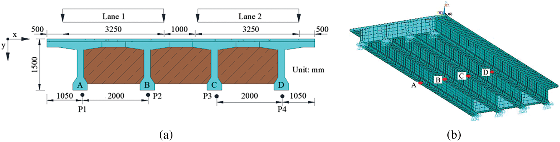
Figure 1: T-girder bridge model (a) cross-section (b) finite element model

2.2.2 Box-Girder Bridge Model

In this study, a box girder bridge with a span of 20 m and a deck width of 11 m was selected to estimate the performance of the pre-trained CNN model after transfer learning. The cross-section of the bridge was shown in Fig. 2a. Similar to the T-girder bridge model, the ANSYS framework was also used to develop the FE model of the box-girder bridge, as shown in Fig. 2b. The bridge deck and the main girders were all simulated by the Solid185 element. The properties of the concrete material used in the box-girder bridge were the same as those adopted in the T-girder bridge.

Figure 2: Box-girder bridge model (a) cross-section (b) finite element model

2.3 Vehicle Bridge Coupled Vibration

In this study, the transverse loading position of the vehicle was randomly generated following a uniform distribution, and the ranges of the transverse loading positions in Lane 1 and Lane 2 were determined by points “P1” to “P2” and points “P3” to “P4”, respectively, as illustrated in Fig. 1a. The strain of the girders was collected from the points at the bottom of each girder in the middle span of the bridge. These points were denoted by “A”, “B”, “C”, and “D” in Figs. 1b and 2b.

In this study, the vehicle bridge coupled vibration system was used to obtain the bridge response under vehicular loading. This system was mainly based on the modal coordinates and used the Newmark-β method to solve the dynamic equation. The comprehensive description of the vehicle bridge coupled vibration system adopted in this study can be found in other literature by the authors [16,17] and was not repeated here. Results obtained from this system have been verified by field tests and were proved to be accurate and reliable.

3  CNN-Based B-WIM Technology

3.1 Training Data Collection

Previous studies have demonstrated that the CNN-based B-WIM technology required a large amount of training data, potentially reaching millions [6]. Hence, it is significant to find a good balance between the training data size and the prediction accuracy when using the CNN technology. In this study, 6000 sets of data collected from the bridge under various loading conditions were used as the training data, and another 1500 sets of strain data were used as the validation data.

The data sampling frequency was set at 1 kHz. The sampling time was determined to be 4 s considering the minimum driving speed. Data gaps resulting from the sampling time less than 4 s were filled with zeros. Additionally, the obtained bridge responses were augmented with 50 decibels of Gaussian white noise to simulate the real noise, and they should be normalized to the values between 0 and 1 before the training of the CNN.

3.2 Development and Optimization of the CNN

It is noted that the bridge responses under vehicular loading can be regarded as a convolutional outcome of the vehicle axle weight and the bridge influence line. This implies that the bridge weigh in motion can be considered as a deconvolution problem. In the bridge dynamic weighing theory, the bridge response was assumed to be obtained under a linear elastic state. The relationship between the bending moment of the bridge and the loaded vehicle was listed as follows:

M(x)=∫I(x)P(x)dx+ε(x)(1)

where M(x) is the measured bending moment; P(x) is the function of the vehicular axle weight; ε(x) is the bending moment in theory, i.e., the difference between ∫I(x)P(x)dx and M(x); I(x) is the influence line of the bridge.

Based on Eq. (1), it was evident that if the influence line of the bridge, the vehicle’s axle load vector, vehicle speeds, and wheelbases were given, the bending moment of the bridge can be determined. The bridge responses were believed to contain sufficient information of the vehicle loading conditions. Conversely, if the measured bending moments of the bridge were known, the axle load, the vehicle speed, and the wheelbase can be theoretically deduced. For example, the signal length of the measured bending moment response indicated the time of the vehicle crossing the bridge, and thereby the vehicle speed. Moreover, vehicles with different wheelbases typically generate bridge responses with distinct characteristics. Considering the remarkable fitting capabilities and significant potentials for signal feature extraction, the CNN model was adopted in this study to predict the vehicle axle weights by mapping the relationship between the bridge response and the vehicle axle weight.

In this study, the proposed CNN consisted of the input layer, convolutional layer, pooling layer, fully connected layer, and the output layer, as listed in Table 1. The convolutional layer was mainly used to extract features related to the vehicle parameters from the input data. The size of the convolutional kernel used in the CNN was presented in Table 1, and the step size was set to be 1. Each variable in the input layer was fed by a 4000 × 1 vector, which denoted the strain signal collected with the acquisition time of 4 s and a sampling frequency of 1 kHz. Considering the negative signal values in the input data, the “Leaky Relu” activation function, which extended the negative interval of the “Relu” activation function, was adopted in this study. After each convolutional layer, a pooling layer followed and was used to reduce the size of the convolutional layer while retaining essential signal characteristics. In this study, the maximum pooling method was used for the pooling layers, and the corresponding parameters were listed in Table 1. The final layers of the CNN model were fully connected layers, which were employed to capture the complex relationship between the axle weight and the feature matrix generated through the convolution of the input signal. The structure of these fully connected layers used herein was similar to that in the common artificial neural network.

It is noted that in Table 1, “(7 × 1 × 16) [2 × 1]” denoted that the number of convolution kernels was 16, the size of the convolution kernel was 7 × 1, and the size of the kernel used for the pooling was 2 × 1. In this study, the weight parameters were generated randomly, and they were adjusted by the Adam algorithm [18], as shown in Eq. (2). Unlike the randomly generated weight parameter, hyperparameters of the CNN were mainly determined manually. In this study, the hyperparameters of the optimal CNN, as shown in Table 1, were determined considering the results in literature [6] and the recognition error.

mt=β1mt−1+(1−β1)⋅∇J(θt)vt=β2vt−1+(1−β2)(∇J(θt))2m¯t=mt1−β1tv¯t=vt1−β2tθt+1=θt−ηv¯t+∈m¯t(2)

where θt is the weight parameter updated in the t round; J(θt) is the loss function; ∇J(θt) is the gradient of the loss function with respect to the weight parameters and bias; η, β1, β2, and ∈ are all predefined constants.

In this study, the CNN model was designed with 5 output variables for each lane and 10 output variables in total, where each output represented an axle weight. For the two-axle and three-axle vehicles used in this study, the number of vehicle axles was lower than five, and the output values for the lacked axles were all filled with zeros. In addition, the number of axles should be obtained in advance and they can be obtained using additional axle detection sensors.

In this study, the mean square error (MSE) was used as the loss function of the convolutional neural network, as shown in Eq. (3). During the training of the CNN model, the MSE curve over 200 epochs was obtained, as shown in Fig. 3.

LMSE=1N∑i=1N(yi−yi∧)2(3)

where N is the number of the output variables; yi and y^i are the true value and prediction of the output, respectively.

Figure 3: MSE curve over 200 epochs

It can be seen from Fig. 3 that the MSE decreased as the epoch increased. However, at the 15th training epoch, the training data loss became lower than the validation data loss, indicating that the CNN was overfitted at this point. In addition, as the training continued, the MSE value gradually approached zero at the 200th training epoch. Finally, the CNN model trained up to 200 training epochs was utilized as the final neural network model to predict the vehicle weights. It is noted that in order to obtain the optimized CNN model, many training strategies were adopted during the model training, such as the adoption of variable learning rates, different batch sizes, and so on.

3.3 Pre-Trained CNN Model Using Transfer Learning

3.3.1 Collection of Training Data

It is noted that the vehicle model used to generate the strain data for test was different from that for training and validation. In this study, a 2-axle vehicle with a gross weight of 518 kN and axle weights of 353 and 165 kN was employed to evaluate the performance of the pre-trained CNN model using transfer learning on another bridge. The comparison of recognition accuracy of CNN models with and without transfer learning was conducted under different amounts of training data. The results were presented in Fig. 4. It is noted that the CNN model after transfer learning was referred to as CNN2 hereafter for simplicity, and the CNN model developed based on the T-girder bridge was denoted by CNN1.

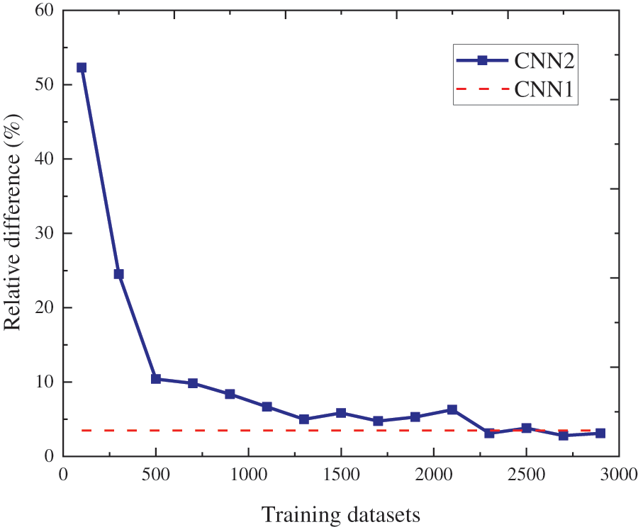
Figure 4: Comparison of the accuracy of CNN1 and CNN2

As shown in Fig. 4, the model’s accuracy steadily improved as the amount of data increased. When the amount of training data reached around 2250 sets, CNN2 provided the comparable accuracy with CNN1. Compared with the amount of training data required by CNN1, i.e., 6000 sets, the appropriate amount of training data for CNN2 model has been reduced by approximately 63%, i.e., 3750 sets, indicating the high potential of transfer learning in reducing the quantity of the training data samples for CNN-based B-WIM methods. In this study, 2250 was finally selected as the amount of data used for CNN2. Similar to CNN1, the validation data for CNN2 was also not included in the training data and accounted for 25% of the training data.

3.3.2 Transfer Learning

Due to the changes in the bridge model and training data, hyperparameters of the original CNN model (i.e., CNN1) may not be optimal for the CNN model using transfer learning (i.e., CNN2). Considering the similar tasks performed by CNN1 and CNN2, the transfer learning was adopted to reuse the elements of the pre-trained CNN1 to reduce the amount of datasets required and improve the training efficiency of CNN2. The procedure of transfer learning applied to the pre-trained CNN1 was shown in Fig. 5.

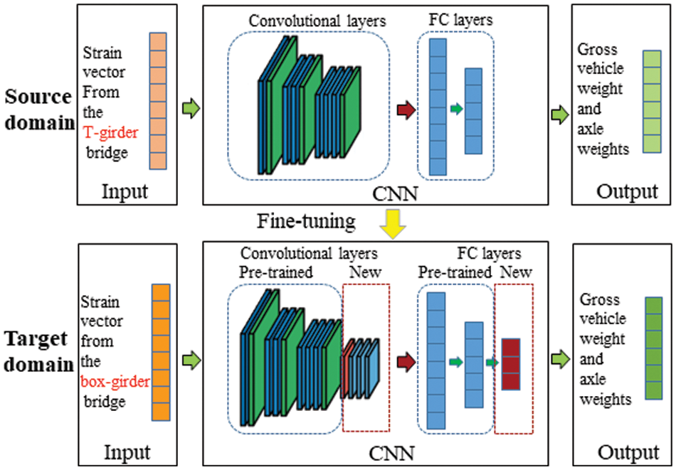
Figure 5: Transfer learning applied to the pre-trained CNN model

It should be noted that the transfer learning was not a machine learning algorithm, but a method to share the generalized knowledge between the models performing similar tasks. In this study, fine-tuning strategy was adopted to adjust the hyperparameters to make CNN2 adapt well to the characteristics of the new bridge response signals. More specifically, in the transfer learning process, all convolutional layers and fully connected layers of the pre-trained CNN1 model were reused and frozen during the training of the pre-trained CNN model, i.e., Convolutional layers 1–9 and Fully connected layers 1–2 as listed in Table 1, and three more new convolutional layers and one more fully connected layer were developed to satisfy the target of CNN2 model for the new bridge. Then the new added convolutional layers and fully connected layer should be trained to obtain the optimized hyperparameters and weights. Finally, the optimal hyperparameters of CNN2 were shown in Table 2. It should be noted that the notation of hyperparameters in Table 2 was consistent with that used in Table 1.

It is emphasized that although the performance of CNN2 was evaluated based on recognition accuracy of the gross weight of a 2-axle vehicle to determine the appropriate amount of training data, the identification results of the axle weight and gross weight of different vehicles under various loading conditions remained unknown. Therefore, further investigations of the recognition accuracy of CNN1 and CNN2 under different loading conditions were necessary.

4  Identification Results Based on CNN1

4.1 Effect of the Loading Route

In this study, 50 2-axle vehicles, 50 3-axle vehicles, and 50 5-axle vehicles that were not included in the train and validation data were selected to investigate the performance of CNN1 under different vehicle loading routes. These vehicles were traveled at a speed of 20 m/s and loaded on Lane 1 along five driving routes that were evenly spaced within the range of “P1” to “P2” with an interval of 0.5 m. Each loading case involved only one vehicle traveling along the bridge. As a result, a total of 750 sets of strain responses were obtained from points A, B, C, and D of the four main bridge girders for further analysis.

The collected bridge responses were then fed to the trained CNN1 to predict the vehicle axle weight and gross weight. The mean value and standard deviation of identified errors of the axle weight of 2-axle, 3-axle, and 5-axle vehicles were presented in Figs. 6 and 7, respectively. Based on Figs. 6 and 7, it was important to note that “#2A1” in the legend denoted the first axle weight of the 2-axle vehicle. “#2” and “A1” referred to the 2-axle vehicle and the weight of the first axle, respectively. The meanings of legends in the following figures can be deduced in a similar manner.

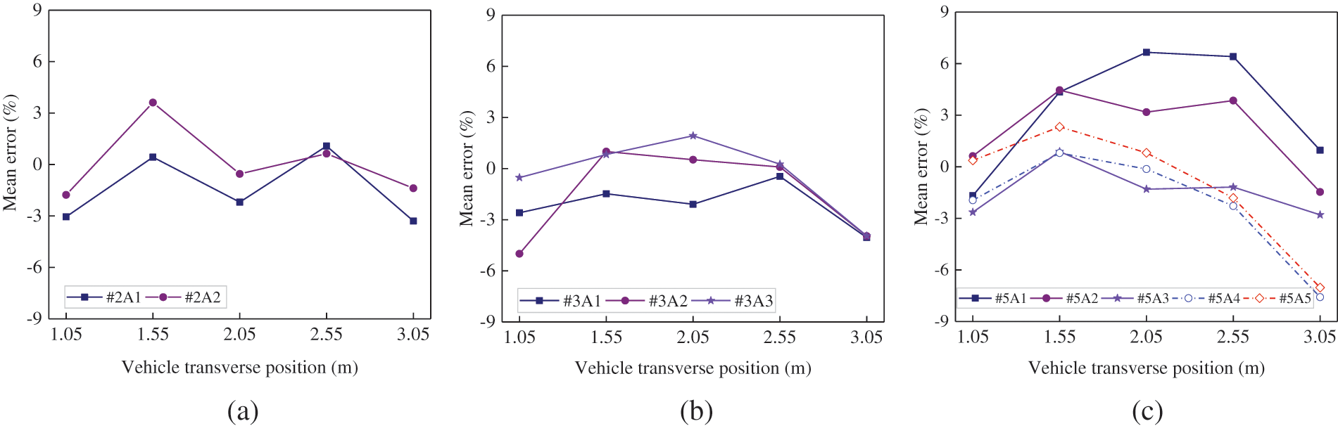
Figure 6: Mean errors of the identified axle weights for (a) 2-axle, (b) 3-axle, and (c) 5-axle vehicles

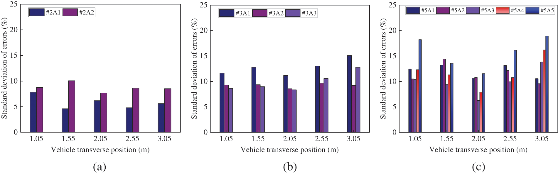
Figure 7: Standard deviation of errors of the identified axle weights for (a) 2-axle, (b) 3-axle, and (c) 5-axle vehicles

As shown in Figs. 6 and 7, the mean absolute values of the axle weight identification errors for 2-axle vehicles were below 4%, and the values of standard deviation were basically below 8%. For 3-axle and 5-axle vehicles, the mean absolute values of the axle weight identification error were all below 5% and 6%, respectively, and the corresponding values of standard deviations were below 12% and 15%, respectively. It was clear that CNN1 exhibited the best recognition performance for 2-axle vehicles, followed by 3-axle vehicles, and then 5-axle vehicles. Although the axle weight identification accuracy and stability slightly decreased with the increase of the number of axles, it still met the precision requirements in practical engineering.

Furthermore, it can be observed from Figs. 6 and 7 that the variation range of the mean values and standard deviations of the axle weight identification errors for each vehicle at different transverse positions were generally below 5%. This phenomenon demonstrated that CNN1 was capable of effectively predicting the axle weights for vehicles traveling along different loading routes.

In this study, the impact of loading routes on the identification accuracy of CNN1 for gross vehicle weight was also investigated. The mean error and standard deviation for 2-axle, 3-axle, and 5-axle vehicles were shown in Fig. 8.

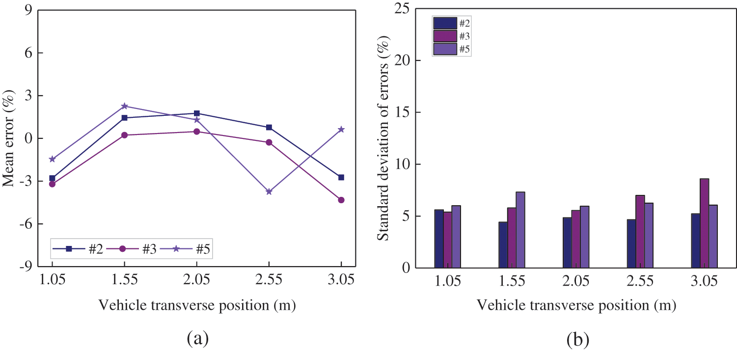
Figure 8: Results of the identified gross vehicle weights: (a) mean error; (b) standard deviation of errors

It can be observed from Fig. 8 that the absolute values of the mean error and standard deviation for the gross weights of all three types of vehicles were typically below 3% and 7.5%, respectively, which were significantly smaller than the corresponding mean values and standard deviations of the axle weight errors, as shown in Figs. 6 and 7, respectively. Therefore, it was believed that CNN1 performed much better in gross weight identification compared to the axle weight identification. Moreover, the standard deviation of identification errors for the gross weight of the 2-axle, 3-axle, and 5-axle vehicles varied by about 1%, 3%, and 1%, respectively, indicating that CNN1 could not only effectively identify the gross weight of different types of vehicles under different loading paths, but also provide stable recognition accuracy.

4.2 Effect of the Traveling Speed

In this study, CNN1’s predictions for vehicle axle weight and gross weight when vehicles passed the bridge along the same loading path but at different speeds were also investigated. Fifty 2-axle vehicles, fifty 3-axle vehicles, and fifty 5-axle vehicles that were not included in the train and validation data were selected. All vehicles loaded at a transverse position of 2.05 m and traveled at speeds of 10, 15, 20, 25, and 30 m/s, respectively. A total of 750 sets of bridge responses under different loading conditions were then obtained. Each loading case involved only one vehicle traveling along the bridge. The collected bridge responses were then fed to CNN1 to predict the vehicle axle weight, and the mean values and standard deviations of the identification errors for axle weight were shown in Figs. 9 and 10.

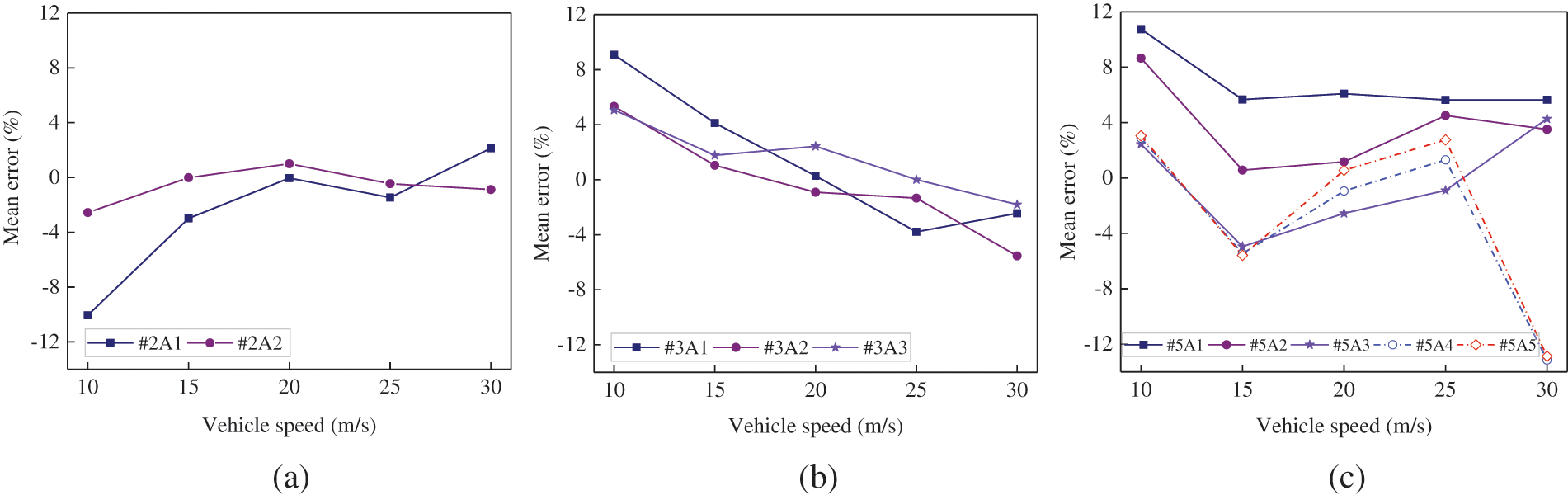
Figure 9: Mean errors of the identified axle weights for (a) 2-axle, (b) 3-axle, and (c) 5-axle vehicles

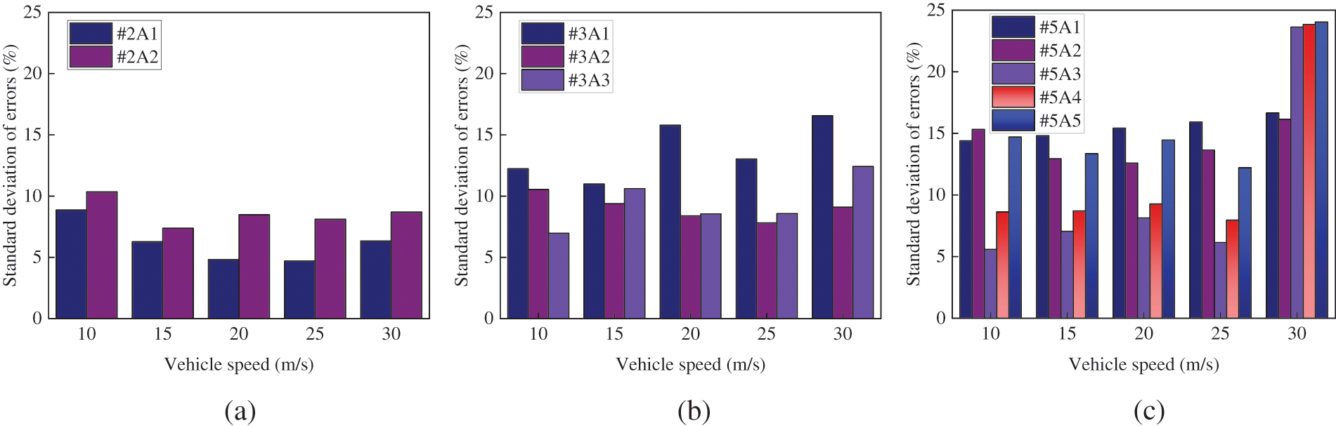
Figure 10: Standard deviation of errors of the identified axle weights for (a) 2-axle, (b) 3-axle, and (c) 5-axle vehicles

Based on Figs. 9 and 10, it can be observed that the CNN-based B-WIM algorithm proposed in this study displayed notable identification errors in predicting axle weights for 2-axle, 3-axle, and 5-axle vehicles traveling at speeds of 10 and 30 m/s. Moreover, for vehicles traveled with speeds ranging from 15 to 25 m/s, the algorithm provided stable and accurate predictions. The lower recognition accuracy of the CNN model under the condition with speeds of 10 and 30 m/s can be attributed to the less amounts of training data with speeds close to the boundary values.

Moreover, it can be observed from Figs. 9 and 10 that the absolute values of axle weight recognition errors for 2-axle and 3-axle vehicles were all below 6%, and the corresponding standard deviation were generally below 12%. For 5-axle vehicles, the absolute values of axle weight recognition errors were typically below 10% and the standard deviations of errors were mostly below 15%. These findings indicated that the CNN model proposed in this study performed better in axle weight identification for the 2-axle and 3-axle vehicles than for 5-axle vehicles. Additionally, the significant variation in the mean error for the axle weights of the 5-axle vehicle can be attributed to the close distance between the fourth and fifth axles. And the close axle distance may result in an interference when identifying these two axle weights, especially under varied speeds.

In this section, Fig. 11 presented the mean value and standard deviation of the gross weight recognition errors from the proposed CNN-based B-WIM algorithm for 2-axle, 3-axle, and 5-axle vehicles at different speeds. The gross weight errors for each type of vehicle followed a similar trend to that of the axle weight errors, and the large absolute values of standard deviation or mean error occurred at speeds of 10 and 30 m/s. However, it is worth noting that the absolute values of the mean errors under all loading conditions remained below 5% in Fig. 11, and the maximum standard deviation of the error was only 8.19%. This indicated that CNN1 performed better in predicting the gross weight than the axle weight for vehicles traveled at different speeds.

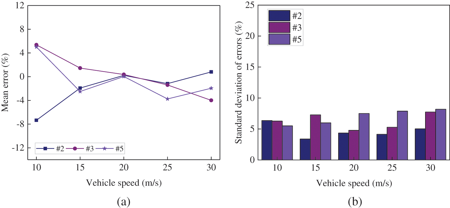
Figure 11: Results of the identified gross vehicle weights (a) mean error; (b) standard deviation of errors

5  Identification Results Based on CNN2

5.1 Effect of the Loading Route

In this section, the performance of the convolutional neural network model through transfer learning, i.e., CNN2, in recognizing the axle weights of vehicles loading at different transverse positions was investigated. For this purpose, the 150 vehicle models for 2-axle, 3-axle, and 5-axle vehicles, as previously employed in Section 4, were adopted to evaluate the recognition accuracy. None of these vehicles were used for training CNN2, and the vehicle speed was 20 m/s for all cases. Since the bridge used for CNN2 and CNN1 had different deck widths (3.75 and 3.25 m, respectively), five new loading routes on the new bridge were selected according to the rule that the five routes were evenly distributed on the selected lane. Finally, the loading routes for the vehicles traveling along the new bridge were determined to be 1.05, 1.71, 2.38, 3.04, and 3.7 m, denoted by “P1”, “P2”, “P3”, “P4”, and “P5”, respectively. For clarity in the following analysis, the corresponding routes denoted by “P1”, “P2”, “P3”, “P4”, and “P5” on the new and original bridge models were listed in Table 3. For example, “P5” denoted the transverse position of 3.7 m on the new bridge and 3.05 m on the original bridge.

In this study, the bridge responses under the loading of the 2-axle, 3-axle, and 5-axle vehicles along different transverse positions were collected. And they were fed to CNN2 to obtain the mean value and standard deviation of the prediction errors for each vehicle’s axle weight, as presented in Table 4. The results were then compared with the recognition accuracy of CNN1 under the same loading conditions. In Table 4, the “Difference” term denoted the differences between the absolute values of mean errors obtained from CNN2 and CNN1. It can be seen from Table 4 that the performance of CNN2 exhibited an evident similarity with CNN1 in terms of the changes of the mean error for identified axle weights. Moreover, CNN2 showed slightly lower prediction accuracy for individual axle weights compared with CNN1, and the axle weight recognition accuracy for other axles of each vehicle model was mostly comparable between CNN2 and CNN1. It should be noted that CNN2 performed very well in recognizing axle weights for each axle of 2-axle vehicles, followed by 5-axle vehicles, and finally 3-axle vehicles. Notably, the mean prediction errors for axle weights of 2-axle and 5-axle vehicles were generally around 3% and 5%, respectively, indicating that CNN2 could identify the axle weights of these vehicle models stably regardless of changes of transverse positions.

In particular, CNN2 showed slightly higher prediction accuracy for the first-axle weight of 3-axle vehicles but lower accuracy for the second-axle weight and third-axle weight compared to CNN1. The most significant difference was observed in prediction accuracy for the third-axle weight, which consistently remained around 10% lower than that of CNN1 at each transverse position. The evident difference can be attributed to the following reasons: First of all, the smaller gradient of the third axle of the 3-axle vehicle led CNN2 to make fewer parameter update during the training using transfer learning. As a result, CNN2 retained more prediction rules learned from CNN1 when identifying the third axle. Furthermore, the stiffness differences between the original bridge and the new bridge led to similar but not identical changes in the collected bridge strain signals. Finally, the overall decline in the mean error for the third axle weight predicted by CNN2 appeared.

In this study, the effect of different loading routes on the recognition accuracy of CNN2 for vehicle gross weight was also evaluated, as shown in Table 5. It can be seen from Table 5 that the recognition accuracy of CNN2 for the gross weight of the vehicle varied slightly under different transverse loading positions and was higher than the prediction accuracy for axle weights. Moreover, CNN2’s recognition accuracy for the gross weight of 2-axle vehicles could match the accuracy of CNN1. For 5-axle vehicles, the recognition accuracy of CNN2 was slightly lower than that of CNN1. While for 3-axle vehicles, there was a significant prediction difference between CNN2 and CNN1, and this discrepancy was primarily due to the prediction error of CNN2 for the 3rd-axle weight of 3-axle vehicles was 10% larger than that of CNN1.

5.2 Effect of the Traveling Speed

In this section, the axle weight recognition accuracy of CNN2 under various operating speeds was investigated using the same vehicle models described in Section 5.1, which included 50 2-axle vehicles, 50 3-axle vehicles, and 50 5-axle vehicles. All vehicles loaded along the centerline of Lane 1 with loading speeds of 10, 15, 20, 25, and 30 m/s.

The bridge strain signals generated by the loading of vehicles at different traveling speeds were fed into CNN2, and the corresponding predictions of the axle weights for 2-axle, 3-axle, and 5-axle vehicles were obtained, as presented in Table 6. Based on Table 6, it was evident that the prediction accuracy of CNN2 for most axle weights was slightly lower than that of CNN1 at different speeds, but still acceptable. At speeds of 10 and 30 m/s, CNN2 showed higher recognition errors for axle weights, similar to CNN1’s results. This phenomenon highlighted the impact of predicting style of the original CNN model on the one through transfer learning when the training data is insufficient. It should be noted that CNN2’s prediction accuracy for the third axle of the 3-axle vehicle at different speeds were generally lower than that of CNN1, which can be due to the similar reason as stated in Section 5.1.

In this study, the recognition performance of CNN2 for the gross weight of vehicles at different speeds was also evaluated, and the mean prediction errors and the differences between the mean errors predicted by CNN2 and CNN1 were presented in Table 7. From Table 7, it can be observed that CNN2 performed much better in recognizing the gross weight of vehicles compared with the recognition results of axle weights. The mean errors for the gross weight of vehicles at all speeds were generally below 5.5% but still slightly higher than that predicted by CNN1. It should be noted that due to the influence of high axle weight errors for the 3rd axle of 3-axle vehicles, CNN2’s recognition performance for the gross weight of 3-axle vehicles was not as good as that for 2-axle and 5-axle vehicles.

In this study, it should be noted that although various traveling speeds and transverse loading positions were carefully considered to evaluate the performance of the proposed CNN model and pre-trained CNN model using transfer learning, not all scenarios considered in this study denoted common loading conditions in the real traffic. For example, the transverse loading positions P1 and P5 denoted that the vehicle traveled along the edge of the lane; the traveling speed of 30 m/s denoted that the vehicle crossed the small bridge as considered in this study with a high speed of 108 km/h. Actually, in the real traffic, vehicles usually traveled near the middle of the lane out of consideration of driving safety and probably traveled in the edge of the lane for temporary overtaking. Moreover, vehicles were more likely to travel with speeds over 80 km/h on highway, instead of on the small bridge as considered in this study. And under the normal loading cases that the vehicles traveled along the path near the middle of the lane and with speeds under 30 m/s, the CNN model could performed well, as can be seen from Figs. 6–11 and Tables 4–7, which indicated that the proposed CNN1 and pre-trained CNN model using transfer learning, i.e., CNN2, were adequate for the load identifications under normal loading conditions in the real traffic.

6  Summary and Conclusions

In this study, the transfer learning-enhanced CNN algorithm for B-WIM technology was proposed with the expectation of a small amount of training datasets, the high identification accuracy, and good applications to weigh different bridges. The recognition accuracy of the developed CNN models, both before and after transfer learning, was evaluated by numerical simulations considering various loading conditions. The conclusions can be drawn as follows:

(1)   The proposed CNN-based B-WIM technology demonstrated good performance in recognizing the axle weight and gross weight of 2-axle and 3-axle vehicles. The mean errors of the axle weight and gross weight were typically below 5% and 3%, respectively. Moreover, the recognition performance was found to be less affected by the vehicle loading route and traveling speed.

(2)   By employing transfer learning, the pre-trained CNN model was successfully applied to the new bridge, resulting in a remarkable 63% reduction in the amount of training data required. This phenomenon demonstrated the effectiveness of transfer learning in reducing the training resources when applying a pre-trained CNN model to different bridges.

(3)   The pre-trained CNN model using transfer learning achieved comparable accuracy to the original one in recognizing the vehicle axle weight and gross weight under different loading routes, demonstrating the promising application potentials of transfer learning. However, the weight recognition accuracy of the pre-trained CNN model based on transfer learning was slightly lower than that of the original model when dealing with different speeds. This phenomenon can be attributed to the insufficient training data with speed near the limit in this study.

(4)   The prediction behavior of the pre-trained CNN model using transfer learning was influenced by the prediction behavior of the original model to some extent. If there is a shortage of training samples, the recognition accuracy may be lower than that of the original CNN model, but the prediction fashion could remain similar to the original one.

It is noted that there is still much progress to be made in the future to improve the performance of the transfer learning-enhanced CNN model, such as the load identification for multiple moving vehicles on the bridge, the performance investigation of the CNN model using transfer learning under high vehicle speeds or insufficient training datasets.

Acknowledgement: The authors gratefully acknowledge the financial support provided by the National Natural Science Foundation of China, the Excellent Youth Foundation of Education Department in Hunan Province, the Xiaohe Sci-Tech Talents Special Funding under Hunan Provincial Sci-Tech Talents Sponsorship Program, and the Science Foundation of Xiangtan University.

Funding Statement: The authors gratefully acknowledge the financial support provided by the National Natural Science Foundation of China (Grant No. 52208213), the Excellent Youth Foundation of Education Department in Hunan Province (Grant No. 22B0141), the Xiaohe Sci-Tech Talents Special Funding under Hunan Provincial Sci-Tech Talents Sponsorship Program (2023TJ-X65), and the Science Foundation of Xiangtan University (Grant No. 21QDZ23).

Author Contributions: The authors confirm contribution to the paper as follows: study conception and design: Xin Luo, Wangchen Yan; data collection: Xin Luo; analysis and interpretation of results: Wangchen Yan, Jinbao Yang; draft manuscript preparation: Wangchen Yan, Jinbao Yang. All authors reviewed the results and approved the final version of the manuscript.

Availability of Data and Materials: Due to a part of the data has been used in another work which has not been published, the data is unavailable now.

Conflicts of Interest: The authors declare that they have no conflicts of interest to report regarding the present study.

References

1. Wu, H., Zhao, H., Liu, J., Hu, Z. (2020). A Filtering-based bridge weigh-in-motion system on a continuous multi-girder bridge considering the influence lines of different lanes. Frontiers of Structural and Civil Engineering, 14, 1232–1246. [Google Scholar]

2. González, A., O’Brien, E. J. (2002). Influence of dynamics on accuracy of a bridge weigh in motion system. Third International Conference on Weigh-in-Motion (ICWIM3), pp. 189–198. Orlando, USA. [Google Scholar]

3. O’Brien, E. J., Quilligan, M. J., Karoumi, R. (2006). Calculating an influence line from direct measurements. Bridge Engineering, 159(1), 31–34. [Google Scholar]

4. Zhu, Y., Sekiya, H., Okatani, T., Yoshida, I., Hirano, S. (2021). Acceleration-based deep learning method for vehicle monitoring. IEEE Sensors Journal, 21(15), 17154–17161. [Google Scholar]

5. Wang, Z., Wang, Y. (2021). Bridge weigh-in-motion through bidirectional recurrent neural network with long short-term memory and attention mechanism. Smart Structures and Systems, 27(2), 241–256. [Google Scholar]

6. Kawakatsu, T., Aihara, K., Takasu, A., Adachi, J. (2018). Deep sensing approach to single-sensor vehicle weighing system on bridges. IEEE Sensors Journal, 19(1), 243–256. [Google Scholar]

7. Wu, Y., Deng, L., He, W. (2020). BwimNet: A novel method for identifying moving vehicles utilizing a modified encoder-decoder architecture. Sensors, 20(24), 7170. [Google Scholar] [PubMed]

8. Wang, H., Nagayama, T., Kawakatsu, T., Takasu, A. (2023). A data-driven approach for bridge weigh-in-motion from impact acceleration responses at bridge joints. Structural Control and Health Monitoring, 2023, 2287978. [Google Scholar]

9. Liu, F., Ye, Z., Wang, L. (2022). Deep transfer learning-based vehicle classification by asphalt pavement vibration. Construction and Building Materials, 342, 127997. [Google Scholar]

10. Tang, Q., Xin, J., Jiang, Y., Zhou, J., Li, S. et al. (2022). Novel identification technique of moving loads using the random response power spectral density and deep transfer learning. Measurement, 195, 111120. [Google Scholar]

11. Harris, N. K., O’Brien, E. J., González, A. (2007). Reduction of bridge dynamic amplification through adjustment of vehicle suspension damping. Journal of Sound and Vibration, 302(3), 471–485. [Google Scholar]

12. Shi, X. M., Cai, C. S. (2009). Simulation of dynamic effects of vehicles on pavement using a 3D interaction model. Journal of Transportation Engineering, 135(10), 736–744. [Google Scholar]

13. Zhang, Y., Cai, C. S., Shi, X. M., Wang, C. (2006). Vehicle-induced dynamic performance of FRP versus concrete slab bridge. Journal of Bridge Engineering, 11(4), 410–419. [Google Scholar]

14. Zhou, Y. F., Chen, S. R. (2015). Fully coupled driving safety analysis of moving traffic on long-span bridges subjected to crosswind. Journal of Wind Engineering and Industrial Aerodynamics, 143, 1–18. [Google Scholar]

15. Miao, T. J., Chan, T. H. T. (2002). Bridge live load models from WIM data. Engineering Structures, 24(8), 1071–1084. [Google Scholar]

16. Yan, W. C., Deng, L., Yin, X. F. (2016). Allowable slope change of approach slabs based on the interacted vibration with passing vehicles. KSCE Journal of Civil Engineering, 20(6), 2469–2482. [Google Scholar]

17. Yan, W., Deng, L., Zhang, F., Li, T., Li, S. (2019). Probabilistic machine learning approach to bridge fatigue failure analysis due to vehicular overloading. Engineering Structures, 193, 91–99. [Google Scholar]

18. Jais, I. K. M., Ismail, A. R., Nisa, S. Q. (2019). Adam optimization algorithm for wide and deep neural network. Knowledge Engineering and Data Science, 2(1), 41–46. [Google Scholar]