Optimal Shape Factor and Fictitious Radius in the MQ-RBF: Solving Ill-Posed Laplacian Problems

1  Introduction

A multiquadric (MQ) radial basis function (RBF)

ϕj=rj2+c2=(x−xjc)2+(y−yjc)2+c2,(x,y)∈Ω,(xjc,yjc)∈Ω~⊃Ω,c∈R+(1)

was used by Franke [1] to interpolate the given scattered data in a bounded domain Ω. Here, rj=(x−xjc)2+(y−yjc)2 is the distance between (x, y) and (xjc, yjc).

The solution for a two-dimensional (2D) problem may be expanded as a linear combination of ϕj, such as u=∑j=1najϕj. The expansion coefficients aj are then determined by the governing equation and boundary conditions. One advantage of the MQ-RBF is that its bases in Eq. (1) involve only the single parameter j for both 2D and three-dimensional (3D) problems. These problems have n unknown coefficients aj. The Pascal polynomial bases have two parameters (i, j) in x iyi−j for the 2D problem, and three parameters (i, j, k) in xiyi−jzj−k for 3D problems. Therefore, for the Pascal polynomial bases, the number of unknown coefficients aij is n(n + 1)/2 for the 2D problem and the number of unknown coefficients aijk is n(n + 1)(n + 2)/6 for the 3D problem.

Kansa [2] first adopted the MQ-RBF to solve partial differential equations (PDEs). However, as n increases, the MQ-RBF becomes increasingly ill-conditioned; hence, Liu et al. [3] proposed a multiple-scale MQ-RBF method to mitigate this ill-conditioning to solve elliptic-type PDEs. The accuracy of the MQ-RBF heavily depends on the shape factor and the number of center points (for which no theoretical optimal value is known); hence, determining the optimal values of parameters is critical [4–7]. When Iurlaro et al. [8] applied an energy based method, Noorizadegan et al. [9] adopted the effective condition number technique to determine the optimal shape factor. Although the original RBF centers in the Kansa method [2] were distributed inside the domain and boundary, researchers later developed the fictitious point method to improve the performance of the MQ-RBF by locating the centers inside a curve enclosing the domain [9,10]. They found that the accuracy is greatly improved if the centers are distributed sufficiently far outside of the problem domain.

The seeking of an optimal value of the shape factor is a tricky problem for determining RBFs for the interpolation of PDE problems [11–15]. In accordance with the linear algebraic theory, Liu [16] asserted that the nonharmonic boundary value problem for the Laplace equation is ill-posed because in the resulting linear system Ax = b, b does not lie in the range space of A; hence, no coefficient vector x exists for the expansion of the solution. Liu [16] enlarged the range space of A and improved the accuracy using hybrid method.

In ϕj, the center points (xjc, yjc) and the shape factor c must be determined; however, simultaneously determining the optimal values of these parameters is difficult. In [17], the optimal shape factor was determined by minimizing the energy gap functional. Many numerical solutions for engineering problems have been obtained through polynomial methods [18–22]. Recently, Oruc [23] developed a local mesh-free radial point interpolation method for solving the Berger equation for thin plates. We intend to improve the polynomial method for solving the nonharmonic boundary value problems of Laplace equation. Briefly, the innovations of this paper are as follows:

•   A novel method was developed to determine both the optimal values of the fictitious radius and shape factor in the MQ-RBF for solving the Laplace equation.

•   A new merit function was derived to determine the optimal values of parameters.

•   The relationship between the maximal projection and the effective condition number was derived for the first time.

•   A highly original idea was used the sample function to compute the merit function.

•   The nonharmonic problem was transformed to the Poisson equation with homogeneous boundary conditions.

•   An optimal polynomial method was developed to solve the nonharmonic problems.

•   Highly accurate solutions for the nonharmonic problems were obtained.

The remaining parts of the paper proceed as follows. In Section 2, we introduce the maximal projection technique. In Section 3, we derive the MQ-RBF and demonstrate that the optimal values of the shape factor and fictitious radius are obtained when a merit function derived from the maximal projection technique is minimized; the section also introduces a novel sample function for calculating the merit function. In Section 4, we present numerical examples of the Dirichlet, mixed, and Cauchy problems of the Laplace equation. In Section 5, we introduce the nonharmonic problem and transform it to the Poisson equation endowed with a homogeneous boundary condition; the section also provides numerical examples that illustrate how solutions are obtained with the optimal MQ-RBF and optimal polynomial method. Finally, in Section 6, we conclude the paper.

2  Maximal Projection

In many applications, an unknown vector x∈Rn that is the output of a linear model must be found. This can be achieved by solving a linear system:

Ax=b,(2)

where A∈Rn×n is the given nonsingular coefficient matrix of the linear model, and b is a given input vector.

We attempt to find the best approximation to b from x by finding the optimal value of the shape factor c in the MQ-RBF, which related to A. The error vector is

e:=b−b⋅y∥y∥y∥y∥,(3)

where we let y = Ax for notational simplicity. By minimizing

minx∥e∥2=minx{∥b∥2−(b⋅y)2∥y∥2},(4)

or maximizing

maxx{(b⋅y)2∥y∥2},(5)

the optimal approximation of x can be found; this is named the maximal projection solution.

Because b is a given nonzero constant vector, we can recast Eq. (5) as

maxx{(b⋅y)2∥b∥2∥y∥2},(6)

which does not affect the solution of x. We then minimize the following merit function:

minx{f=∥b∥2∥y∥2(b⋅y)2},(7)

which is the reciprocal of Eq. (6).

By applying Eq. (7), Liu [24] developed efficient methods to solve Eq. (2) iteratively. Liu [24] employed a scaling invariant property of Eq. (7) (i.e., y and βy, leading to the same value of f if β ≠ 0) to derive a maximal projection solution in an affine Krylov subspace and proved that Eq. (7) implies the least-squares solution.

3  Optimal Shape and Fictitious Radius

Consider

∂2u(x,y)∂x2+∂2u(x,y)∂y2=0,(x,y)∈Ω,(8)

u(x,y)=h(x,y),(x,y)∈Γ,(9)

where Γ := { r = ρ(θ), 0 ≤ θ ≤ 2π} is the boundary of a bounded domain Ω, and ρ(θ) is a radius function of Γ that encloses Ω.

In the MQ-RBF method, the trial solution u(x, y) of Eqs. (8) and (9) is given by

u(x,y)=∑k=1nak(x−xkc)2+(y−ykc)2+c2,(10)

where (xkc,ykc), k = 1, …, n are center points given in the Appendix. We have n = m10 × m20 center points that are located inside a circle with a given fictitious radius D. D is a constant radius parameter, and c is a constant shape factor; they both greatly influence the performance of the MQ-RBF. Recently, various techniques for generating center points have been proposed, such as those based on Halton points [9] and Padua points [25].

By considering Eqs. (10), (8), and (9) at nq = m1 × (m2 − 1) + nb collocation points, we obtain

Ga=b,(11)

where a: = (a1,…, an)T, and the components Gij of G and bj of b are given in the Appendix. The first part generates linear equations from the governing equation, whereas the second part generates linear equations from the boundary condition. The dimension of G is nq × n, and Eq. (11) with n = nq can be used to find a. In general, we first select m10 and m20; then, n = m10 × m20. Next, nb = n − m1 × (m2 − 1) can be computed, where m10 × m20 > m1 × (m2 − 1).

To make Eq. (11) less ill-posed, we suggest the multiple-scale MQ-RBF in [3]

u(x,y)=∑k=1naksk(x−xkc)2+(y−ykc)2+c2(12)

as a trial solution. The multiple-scale coefficients sk are determined by

sk=∥G1∥∥Gk∥,(13)

where s1 = 1 and Gk denotes the kth column of G.

Upon letting

A=GD,D:=diag(s1,…,sn),(14)

we obtain a new n-dimensional square linear system:

Aa=b.(15)

D in Eq. (14) acts as a postconditioner to ensure that A is better conditioned than is G. When n is not sufficiently large, we can employ the Gaussian elimination method to calculate the expansion coefficients in a.

To determine the optimal value of shape factor c, let

y=Aa.(16)

Inserting Eq. (16) and b into Eq. (7), we can minimize

minc∈[a,b]{f=∥Aa∥2∥b∥2(b⋅Aa)2}(17)

in a given interval [a, b] by the one-dimensional golden section search algorithm (1D GSSA) with a loose convergence criterion of ε1 = 10−2. When the optimal shape factor has been obtained, the numerical solution in Eq. (12) can be obtained by inserting the shape factor into Eq. (15) and solving for a.

In Eq. (17), the exact a is not yet known. As is the case in [7], we suppose a sample solution us(x, y) that satisfies the Laplace equation but not the boundary conditions. Many polynomial functions automatically satisfy the Laplace equation, such as the two simple sample functions of us(x, y) = x + y and us(x, y) = xy, which are, respectively, the first-order and second-order solutions of Laplace equation. We then interpolate us(x, y) with the bases ϕj at n collocated points (xks,yks) on Ω¯:

us(xks,yks)=∑j=1na^j(xks−xjc)2+(yks−yjc)2+c2,k=1,…,n.(18)

Because us(x, y) is a simple function, we can compute a^=(a^1,…,a^n)T from the linear system (18) rapidly; this is then inserted into Eq. (17) to compute f:

minc∈[a,b]{f=∥Aa^∥2∥b∥2(b⋅Aa^)2}.(19)

A is still computed with Eq. (14), which has c as one of its parameters. Liu et al. [17] determined the optimal shape factor by using the energy gap functional; however, this method is more complicated than the method of using the merit function f here.

To determine D and c simultaneously, we can consider the minimization

min(c,D)∈[a1,b1]×[a2,b2]{f=∥Aa^∥2∥b∥2(b⋅Aa^)2},(20)

which can be performed by the 2D golden section search algorithm (GSSA) with a loose value of ε2 = 10−2. The 1D GSSA in Tsai et al. [26] is much simpler than the 2D case. In general, for high-dimensional search algorithms, the obtained minimum is normally a local minimum and not the global minimum. A is still computed by Eq. (14), involving c and D as parameters. Solving Eq. (20), we can determine the optimal values of c and D. This method is called the optimal MQ-RBF. The GSSA was used by Tsai et al. [26] to find a good shape factor.

Remark 1. Recently, Noorizadegan et al. [9] demonstrated that the effective condition number can provide a much better estimation of the actual condition number of the resultant matrix-vector system (15), and they proposed applying the effective condition number as a numerical tool to determine a reasonably good shape factor in the MQ-RBF. Eq. (15) in [9] is

κκeff=σ1∥a∥∥b∥,(21)

where κ is the traditional condition number, κeff = ∥b∥/(σn∥a∥) is the effective condition number, and σ1 and σn are, respectively, the largest and smallest singular values of A.

Let us estimate the maximal projection (MP) in Eq. (6) denoted as

F=max(b⋅Aa)2∥Aa∥2∥b∥2=max1f.(22)

We choose Aa = σ1a in the numerator and Aa = σna in the denominator; we can thus obtain the largest value of F. We then have

F=σ12α2σn2∥a∥2∥b∥2.(23)

where α2 = (a⋅b)2 is some positive constant. Defining κ = σ1/σn,

F=κ2α2∥a∥2∥b∥2.(24)

In combination with Eq. (21), we can derive

F=α2∥a∥2∥b∥2κeff2σ12∥a∥2∥b∥2=α2σ12κeff2∥b∥4.(25)

The coefficient preceding κeff2 is some constant C=α2σ12/∥b∥4.

Therefore, the minimization in Eq. (17) is equivalent to the maximization of the effective condition number. Noorizadegan et al. [9] found that the shape factor c corresponding to the maximum effective condition number resulted in the numerical solution with the smallest error. This observation is consistent with the presented formulation resulting from this MP-based technique.

We have thus demonstrated that the shape factor obtained with our MP technique and the previous effective condition number technique are equally effective. However, our strategy of selecting the optimal shape factor is much simpler. The computational cost of finding the optimal (c, D) is low because a^ in Eq. (20) is computed from the data interpolation (18) by a given sample function us(x, y).

4  Numerical Examples

We assess the errors of u(x,y),(x,y)∈Ω¯ in terms of the maximum error (ME) and root-mean-square-error (RMSE) as follows:

ME ofu(x,y):=max(x,y)∈Ω¯|ue(x,y)−uN(x,y)|,(26)

RMSE ofu(x,y):=1Nt∑j=1Nt[ue(xj,yj)−uN(xj,yj)]2,(xj,yj)∈Ω¯,(27)

where ue and uN denote the exact and numerical solutions, respectively. Fig. 1 presents plots of the ME with respect to θ, which are obtained as follows:

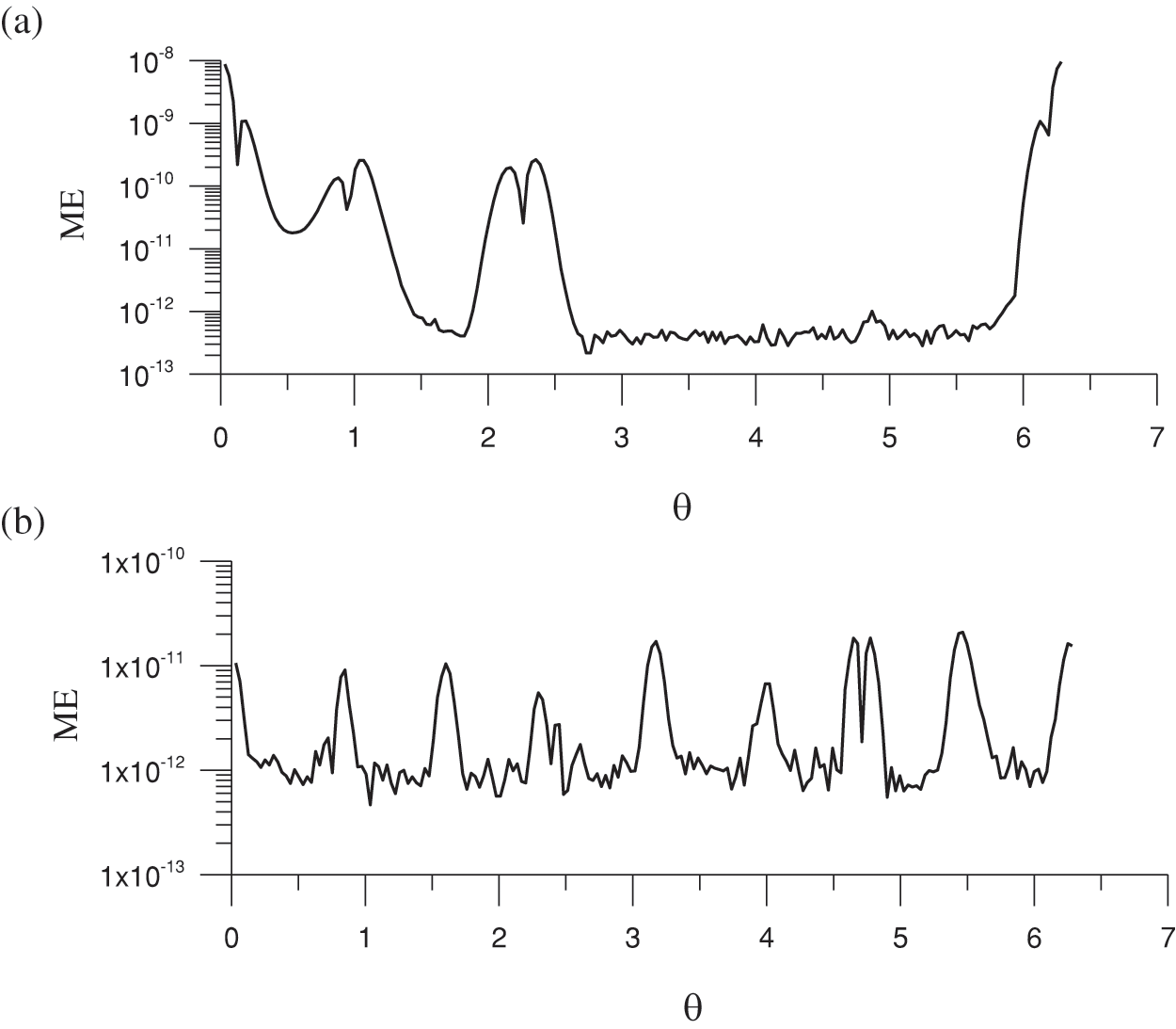
Figure 1: MEs of the solutions for the sample function us = xy with (a) u(x, y) = x2 − y2 and (b) u (x, y) = cosx sinhy + sinx coshy

Maximum error ofu(θ):=maxri≤ρ(θ)|ue(ri,θ)−uN(ri,θ)|,ri=iρ(θ)/n2.(28)

we selected Nt = n1 × n2 = 100 × 20 = 2000.

4.1 Example 1

We consider the following two exact solutions of the Laplace equation:

u(x,y)=x2−y2,(29)

u(x,y)=cos⁡xsinh⁡y+sin⁡xcosh⁡y.(30)

The corresponding boundary shapes are, respectively,

ρ(θ)=exp⁡(sin⁡θ)sin2⁡(2θ)+exp⁡(cos⁡θ)cos2⁡(2θ),(31)

ρ(θ)=1+cos2⁡(4θ)2.(32)

This example is simple; however, we use it to demonstrate the performance of the proposed method. For Eqs. (29) and (31), we take n = 512, nb = 112 and D = 7 to obtain c. We test two sample functions, us = x + y and us = xy. In the interval [a, b] = [1, 1.5] with us = x + y, the optimal value c = 1.309 is obtained after ten iterations in the GSSA for ε1 = 10−2. The ME and RMSE of the numerical solution compared with u(x, y) = x2 − y2 in the entire domain are 5.14 × 10−8 and 2.28 × 10−9, respectively. Moreover, computing the optimal value of c required only 5.35 s of CPU time; the condition number was 5.7 × 107.

Similarly, for us = xy and [a, b] = [1, 3], the optimal value c = 2.235 was obtained within 13 iterations, and ME = 9.59 × 10−9 and RMSE = 3.87 × 10−10 were obtained. Fig. 1a presents a plot of the ME at each angle θ ∈ [0, 2π]. For this solution, the CPU time was 5.31 s, and the condition number was 8.75 × 106. Hence, highly accurate solutions can be generated from both us = x + y and us = xy, despite the substantial difference between c = 1.309 and c = 2.235. Moreover, neither condition number is too large. Unless otherwise specified, we employ us = xy as the sample function in the following computations.

For a fixed interval of [a, b], we, in general, can obtain a local minimum in that interval by using the GSSA. To obtain the global minimum, we can search in various intervals and compare the minimums of each sub-interval to identify the global minimum. However, this technique is time-consuming. For a large interval [a, b] = [1, 5], the results for c, ME, RMSE and the condition number (CN) are listed in Table 1. The result obtained with a large interval [a, b] = [1, 5] (c = 3.505) is more accurate than that obtained by picking the smallest of the local minimums at four subintervals (c = 3.764). This suggests that the MQ-RBF is sensitive to the value of the shape factor c. Therefore, we selected a suitable interval by performing some trials; the interval must be sufficiently large.

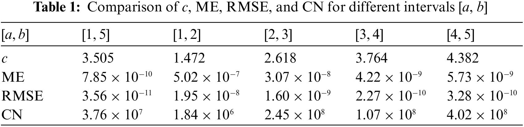
This example allows us to discuss the role of D in Eq. (14). If we take D = I n in Eq. (14), the linear system (15) is not regularized by the multiple-scale coefficients. For D = In, the ME = 6.19 × 10−8 and RMSE = 2.72 × 10−9 are larger than the ME = 9.59 × 10−9 and RMSE = 3.87 × 10−10 obtained by the regularization method.

For Eqs. (30) and (32), changing the values to n = 450, nb = 210, D = 7, and [a,b] = [1, 2], we obtained a proper value c = 1.416 with 11 iterations in the GSSA. If u(x, y) = cosx sinhy + sinx coshy, the ME was 2.09 × 10−11 and the RMSE was 1.9 × 10−12. Fig. 1b presents a plot of the ME for each angle θ ∈ [0, 2π]. The CPU time was 3.31 s, and the CN was 2.48 × 107.

Table 2 presents the accuracy for various D values with the other parameters held constant.

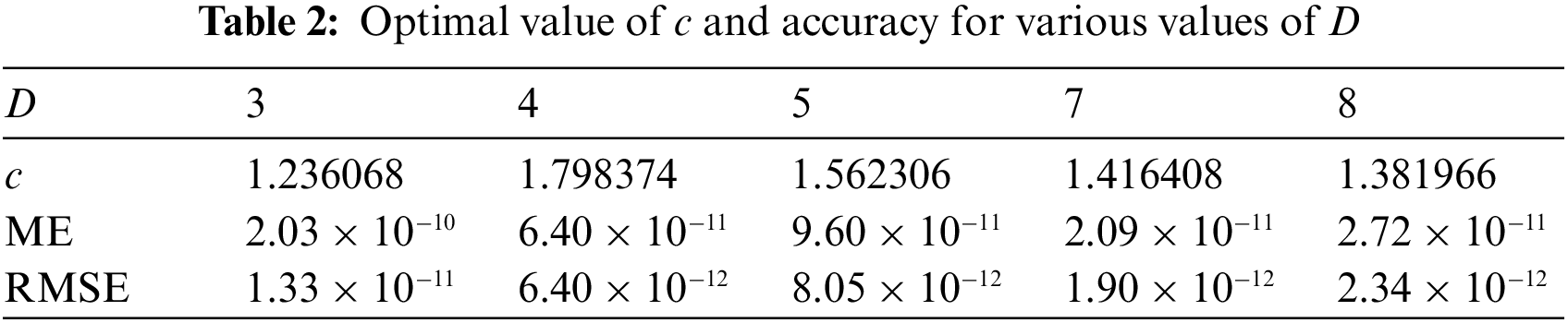
Table 2 reveals that D affects c, the ME, and the RMSE. Hence, to enhance the accuracy, we can apply Eq. (20) to select the optimal values of both c and D.

For n = 512 and nb = 112 in the range [a1, b1] × [a2, b2] = [1, 3] × [6, 8], the optimal values of c = 2.52 and D = 7.176 were obtained with 13 iterations of the GSSA for ε2 = 10−2. Compared with u(x, y) = x2 − y2, ME = 6.51 × 10−9 and RMSE = 2.59 × 10−10; hence, the accuracy is higher than if only c was optimized. Because both the optimal values of c and D were computed, the CPU time increased to 18.15 s. The CN was 4.8 × 107. If the range is enlarged to [a1, b1] × [a2, b2] = [1, 5] × [1, 10], we obtain c = 4.086 and D = 6.52; however, ME = 7.55 × 10−9 and RMSE = 4.04 × 10−10, which are slightly larger than those for the smaller range. For the larger range, the CPU time increased to 21.91 s, and the CN decreased to 3.91 × 107.

For the sample function us(x, y) = excosy in the range [a1, b1] × [a2, b2] = [1, 2] × [6, 8], the optimal values of c = 1.212 and D = 6.996 were obtained with 10 iterations in GSSA for ε2 = 10−2. Compared with u(x, y) = cosx sinhy + sinx coshy, ME = 1.92 × 10−11 and RMSE = 1.84 × 10−12; this was again more accurate than when only c was optimized. The CPU time was 9.76 s, and the CN was 1.15 × 107.

4.2 Example 2

We consider the mixed BVP with two solutions given by Eqs. (29) and (30):

u(x,y)=h(x,y),(x,y)∈Γ1,(33)

un(x,y)=g(x,y),(x,y)∈Γ2,(34)

where Γ1:={r=ρ(θ),0≤θ≤π}, Γ2:={r=ρ(θ),π<θ<2π}, and un(ρ,θ) is the normal derivative of u on the boundary Γ2. The boundary shapes are still given by Eqs. (31) and (32).

For the first mixed BVP, we fix n=512 and nb=112 and seek the proper values of c and D in the range [a1,b1]×[a2,b2]=[1.5,1.9]×[8.1,9.5]. The optimal values c=1.847 and D=9.445 were obtained after 12 iterations, and ME = 7.21×10−9 and RMSE = 4.06×10−10 relative to u(x,y)=x2−y2. The CPU time was 20.47 s, and the CN was 3.56×107.

For the second mixed BVP, we fix n=450 and nb=210, and in [a1,b1]×[a2,b2]=[1,1.5]×[7,8], we obtain the optimal values c=1.335 and D=7.705 with 11 iterations in GSSA under ε2=10−2. ME = 5.33×10−11, and RMSE = 3.13×10−12. The CPU time was 13.29 s, and the CN was 2.31×108.

4.3 Example 3

A Cauchy inverse boundary value problem with two solutions given by Eqs. (29) and (30) can be formulated as follows:

u(x,y)=h1(x,y),un(x,y)=h2(x,y),(x,y)∈Γ1,(35)

u(x,y)=g(x,y),(x,y)∈Γ2,(36)

where g(x, y) is an unknown function to be recovered. We add noise as follows:

h^1=h1(x,y)+sR(x,y),h^2=h2(x,y)+sR(x,y),(x,y)∈Γ1,(37)

where R indicates random numbers with zero mean.

For the first Cauchy problem we fix n=250, nb=170 and s=0.1, and seek the proper values of c and D in the range [a1,b1]×[a2,b2]=[0.5,1]×[6,8]. The optimal values c=0.803 and D=6.468 were obtained with 13 iterations in GSSA under ε2=10−2. ME = 1.65×10−2 and RMSE = 6.7×10−3 were obtained with reference to u(x,y)=x2−y2 on Γ2. In Fig. 2a, we present a comparison of the numerical and exact values for g in the range θ∈[π,2π].

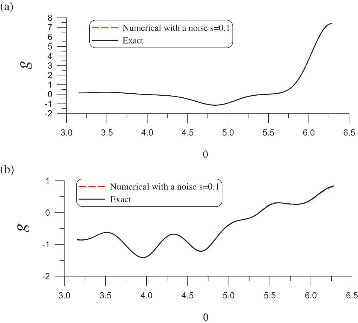
Figure 2: Comparison of the numerical and exact solutions on the lower half boundary for the Laplace equation with Cauchy boundary conditions on the upper half boundary. Solutions for (a) Eqs. (29) and (b) (30)

The optimal values c=0.856 and D=7.743 were obtained for the second Cauchy problem. ME = 1.99×10−2 and RMSE = 8.14×10−3 were obtained, and the numerical and exact values of g in the range θ∈[π,2π] are compared in Fig. 2b. For the ill-posed Cauchy problem, the optimal MQ-RBF is highly accurate even in the presence of substantial noise.

Remark 2. Because the distance function is used in the MQ-RBF, the proposed method is easily extended to 3D problems by taking rj:=(x−xjc)2+(y−yjc)2+(z−zjc)2. However, this may be accompanied by a considerable increase in CPU time. MQ-RBF is known to have a conditionally positive definite kernel; hence, the invertibility of the resulting interpolation matrix is not guaranteed unless the MQ interpolation is augmented with a polynomial basis. In a future study, we may extend the proposed method to Gaussians or inverse MQ-RBFs and to 3D problems.

5  Nonharmonic Boundary Value Problems

In this section we examine the nonharmonic problem of Eqs. (8) and (9), where

∂2h(x,y)∂x2+∂2h(x,y)∂y2≠0,(x,y)∈Ω¯.(38)

The nonharmonic problem comprises Eqs. (8), (9) and (31), where h(x,y)=x2y3 is a benchmark problem. Liu [16] developed a hybrid method denoted MMM for this benchmark problem and obtained a favorable result.

Let

v(x,y)=h(x,y)−u(x,y)(39)

be a new variable; we can then obtain the Poisson equation with a homogeneous boundary condition:

Poisson equation:{Δv=p(x,y),v(x,y)|(x,y)∈Γ=0,(40)

where p(x,y)=Δh(x,y)=6x2y+2y3≠0, because h(x,y) is a nonharmonic function. When v(x,y) has been solved, we can find u(x,y)=h(x,y)−v(x,y).

We first apply the optimal MQ-RBF to solve this nonharmonic problem; the results are presented in Fig. 3. We fix n=525 and nb=445 and seek the proper values of c and D in the range [a1,b1]×[a2,b2]=[0.9,1.8]×[3,6]. The optimal values c=0.901 and D=3.004 were obtained with 13 iterations in GSSA with ε2=10−2. Remarkably, ME = 1.77×10−8 and RMSE = 5.35×10−9 compared with h(x,y)=x2y3 on Γ. Fig. 3a presents a comparison of the numerical and exact solutions in the range θ∈[0,2π]; the errors are plotted in Fig. 3b. We placed many more points on the boundary than that in the interior; this can enhance the accuracy.

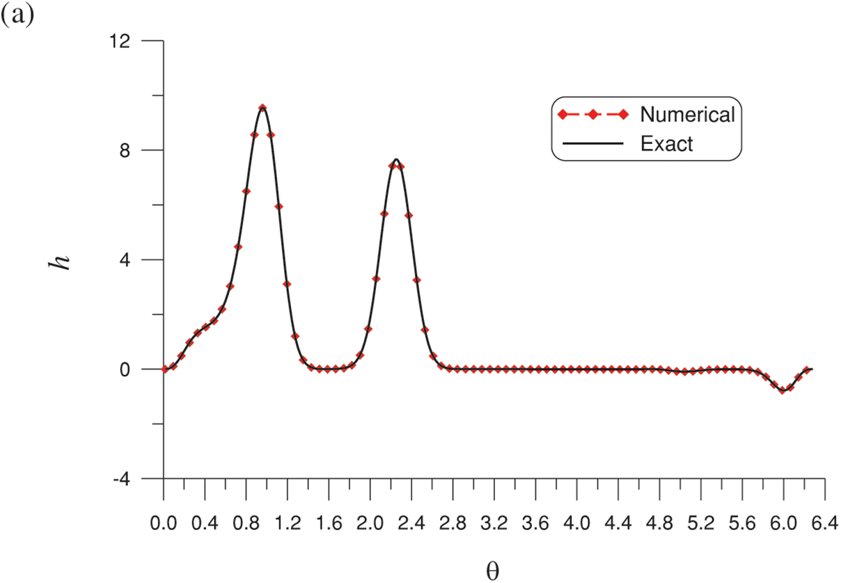
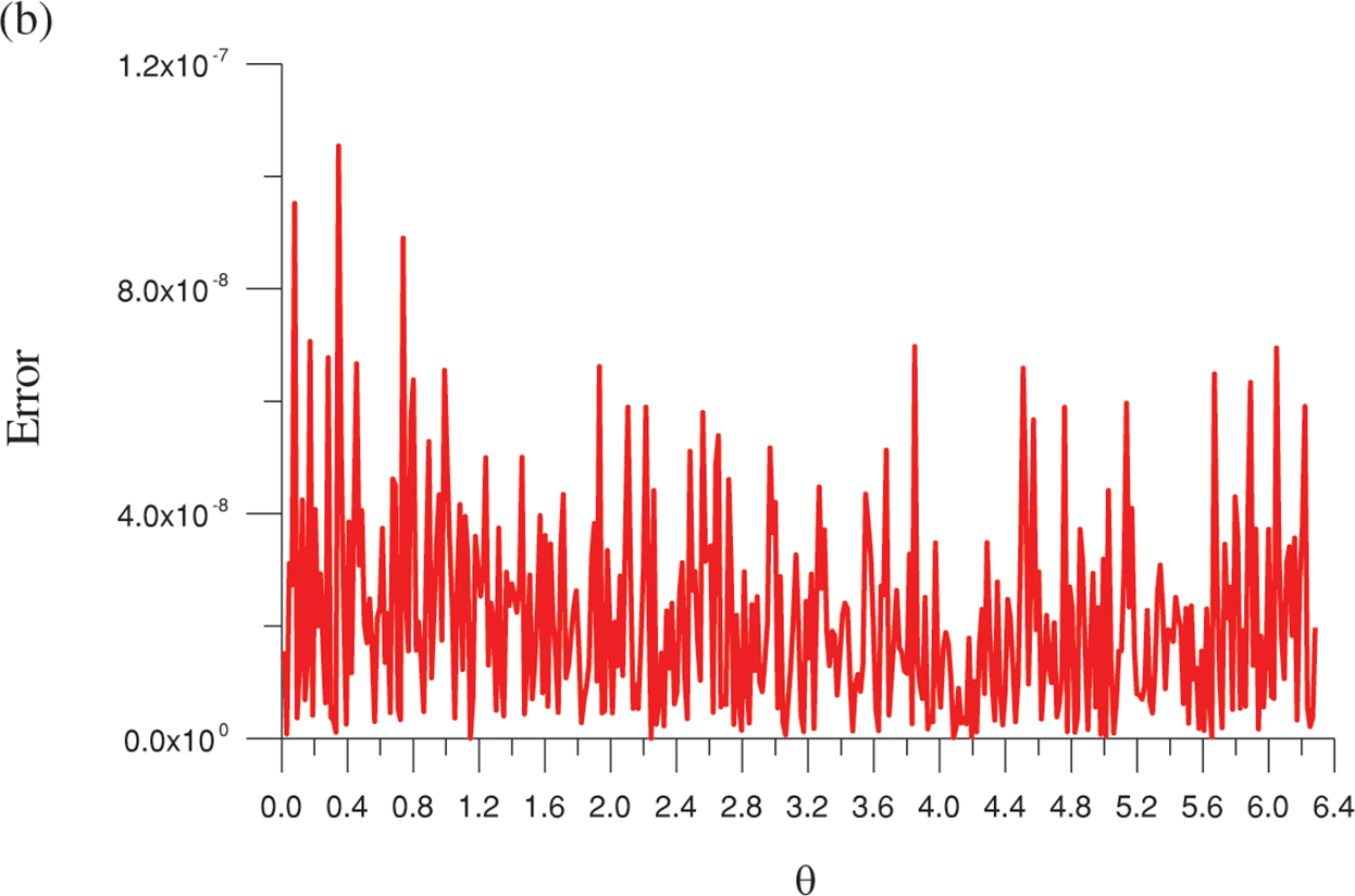
Figure 3: Results for the Laplace equation under a nonharmonic boundary condition on an amoeba shape solved by the optimal MQ-RBF. (a) Comparison of the numerical and exact solutions on the boundary and (b) absolute errors

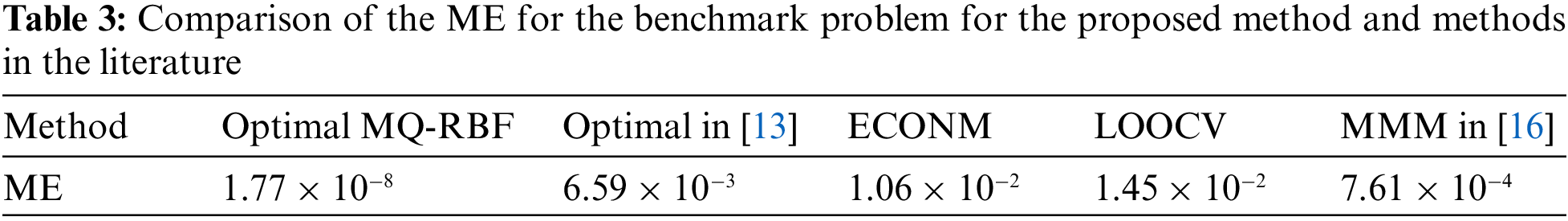
Table 3 presents a comparison of the MEs of the proposed method and methods in previous studies [13,16]. The optimal MQ-RBF outperforms other methods in terms of accuracy by four to six orders of magnitude.

To obtain a more accurate solution for v(x,y) and hence u(x,y)=h(x,y)−v(x,y), we consider the multiple-scale Pascal triangle polynomial expansion method developed by Liu et al. [18]:

v(x,y)=∑i=1m∑j=1icijsij(xR0)i−j(yR0)j−1.(41)

After collocating nq points to satisfy the governing equation and boundary condition (40), we have a non-square linear system (15) for which the scales sij are determined such that each column of the coefficient matrix A has the same norm. Similarly, we can employ the following minimization:

minR0∈[a,b]{f=∥Aa^∥2∥b∥2(b⋅Aa^)2}(42)

to determine the optimal value of R0. We apply the GSSA to solve this minimization problem with a convergence criterion ε1=10−4.

Using the optimal polynomial method (OPM), we first test a direct problem in Eqs. (30) and (31). We take m=15, nq=130×5=650, and [a,b]=[1,5]. The optimal value R0 = 1.000024 was obtained after 24 iterations. For 2000 inner test points, ME = 2.56 × 10−7 and RMSE = 1.62 × 10−8.

For the nonharmonic boundary value problem, we fix h(x,y)=x2y3 and consider the domains with the following shapes:

Five−star:ρ(θ)=1+cos2⁡5θ2,(43)

Peanut:ρ(θ)=cos⁡(2θ)+1.1−sin2⁡(2θ),(44)

Amoeba:ρ(θ)=exp⁡(sin⁡θ)sin2⁡(2θ)+exp⁡(cos⁡θ)cos2⁡(2θ).(45)

For the five-star shape, we use the new OPM with m=10, nq=100×4=400 and [a, b] = [500, 1500]. After 34 iterations, the optimal R0 = 1450.829 was obtained. The results are presented in Fig. 4a, and the corresponding errors are plotted in Fig. 4b. For 400 test points on the boundary, ME = 5.85×10−11 and RMSE = 2.68×10−11 are countered.

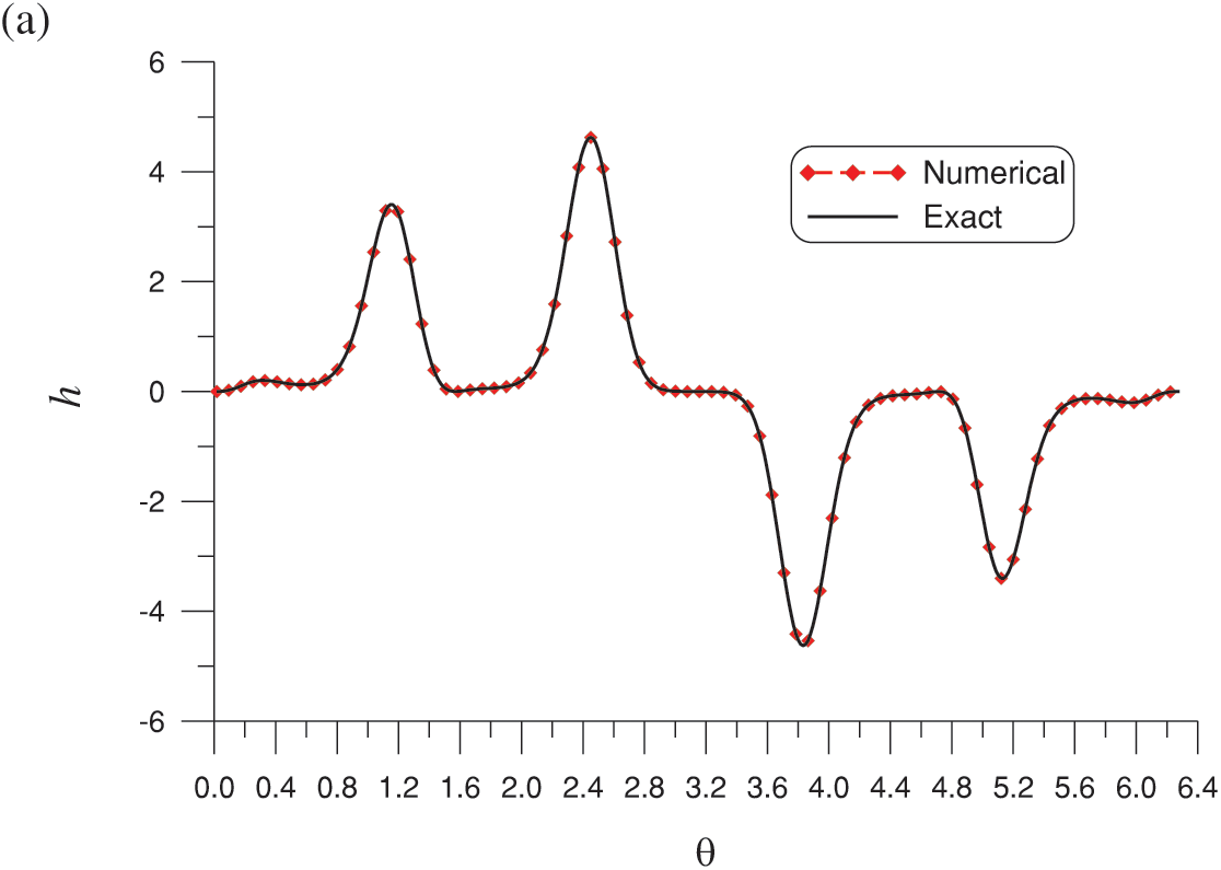
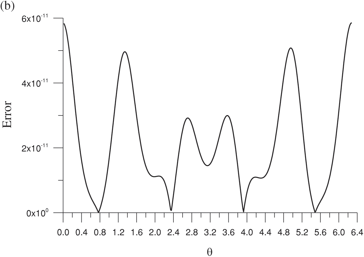
Figure 4: (a) Comparison of the numerical and exact solutions on the boundary and (b) absolute errors for the Laplace equation with a nonharmonic boundary condition and a five-star shape

To apply the new OPM for the nonharmonic problem with a peanut shape, we take m=6, nq=100×4=400, and [a,b]=[10,1500]. After 34 iterations, the optimal R0=1365.607 was obtained. The results are presented in Fig. 5a, and the corresponding errors are plotted in Fig. 5b; ME = 3.83×10−13, and RMSE = 1.34×10−13.

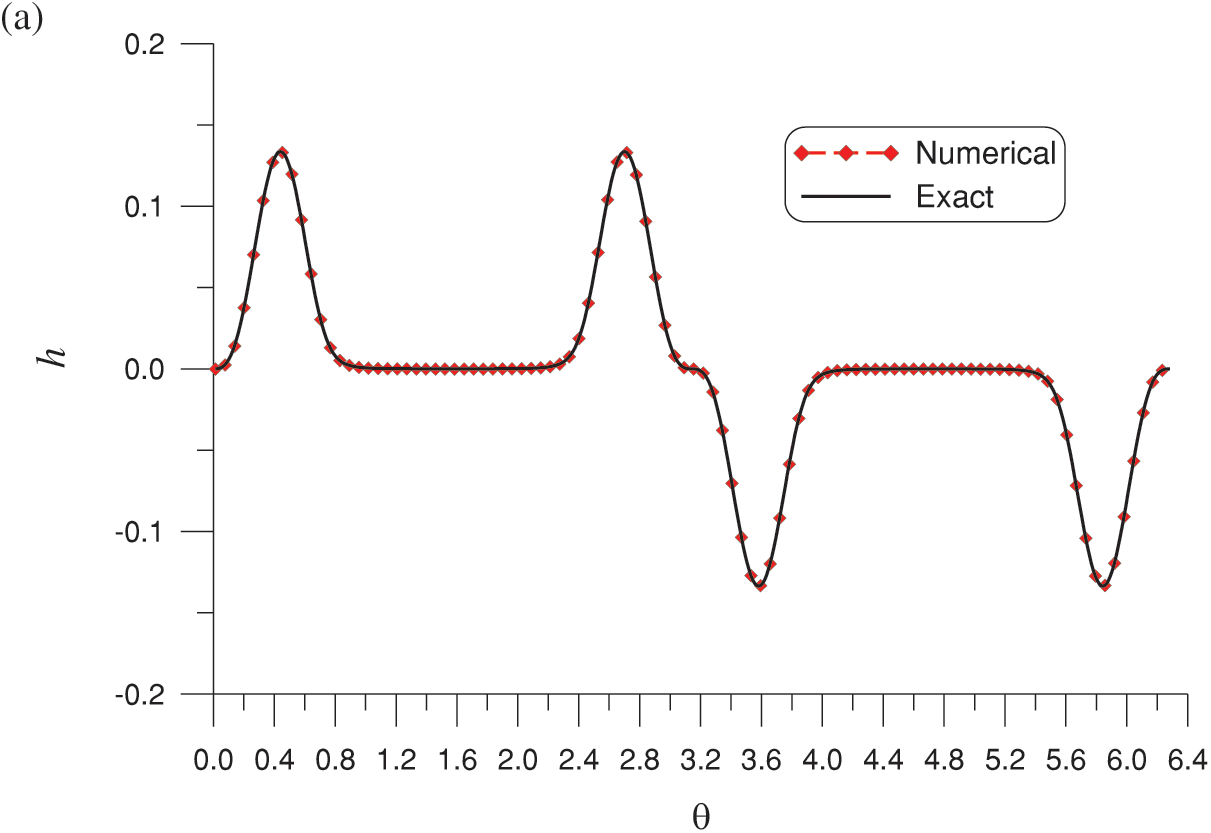
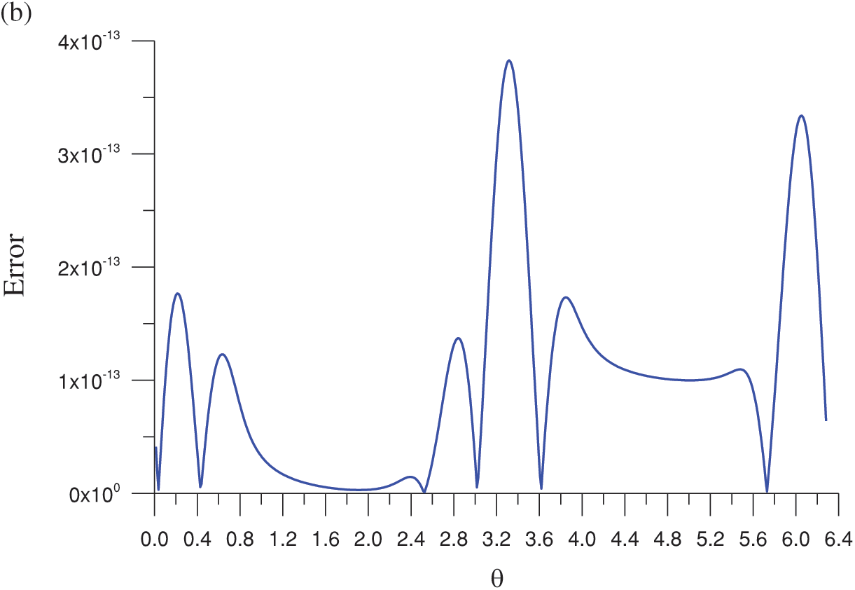
Figure 5: (a) Comparison of the numerical and exact solutions on the boundary and (b) absolute errors for the Laplace equation with a nonharmonic boundary condition and a peanut shape

To apply the OPM for the nonharmonic problem with an amoeba shape, we take m=10, nq=100×4=400, and [a,b]=[1000,1500]. After 30 iterations, the optimal R0 = 1398.8204 was obtained. The results are presented in Fig. 6a, and the corresponding errors are plotted in Fig. 6b; ME = 2.39×10−11, and RMSE = 9.76×10−12. The accuracy is three orders of magnitude better than that from the optimal MQ-RBF (Fig. 3).

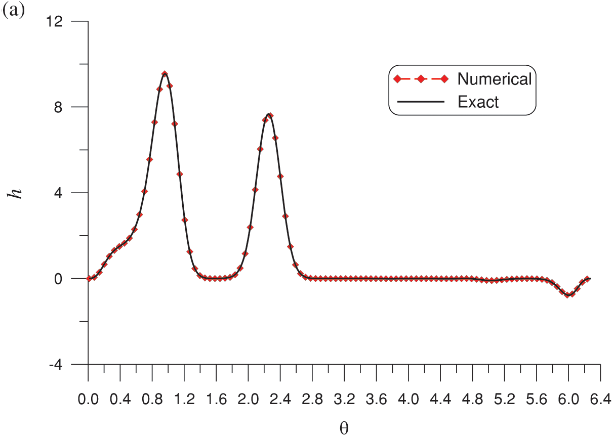
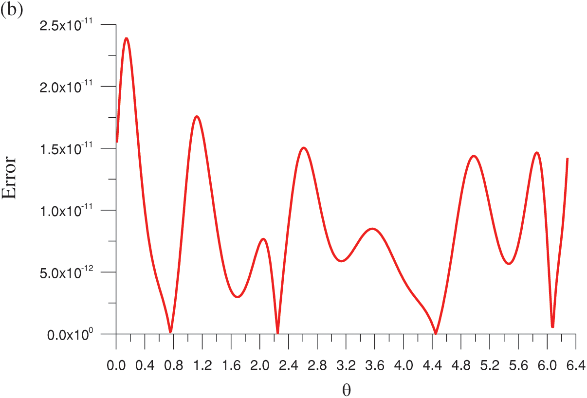
Figure 6: (a) Comparison of the numerical and exact solutions on the boundary and (b) absolute errors for the Laplace equation with a nonharmonic boundary condition and an amoeba shape

For a benchmark problem, the OPM achieves an accuracy of the 11th order; this is far superior to results in the literature with 3rd-order accuracy [13]. The instances of [a, b] of [1, 5], [500, 1000], [10, 1500], and [1000, 1500] used for the different problems were configured to be sufficiently large to ensure that the solutions had high accuracy; this was achieved through trial and error.

Finally, we compared the performance of the OPM and the optimal MQ-RBF for a nonpolynomial nonharmonic function h(x,y)=sin⁡xcos⁡y on a peanut shape.

For the OPM, we take m=15, nq=100×4=400, and [a,b]=[1000,1500]. After 32 iterations, the optimal R0=1072.076 was obtained. The results are presented in Fig. 7a, and the corresponding errors are plotted in Fig. 7b; ME = 5.86×10−12 and RMSE = 2.5×10−12.

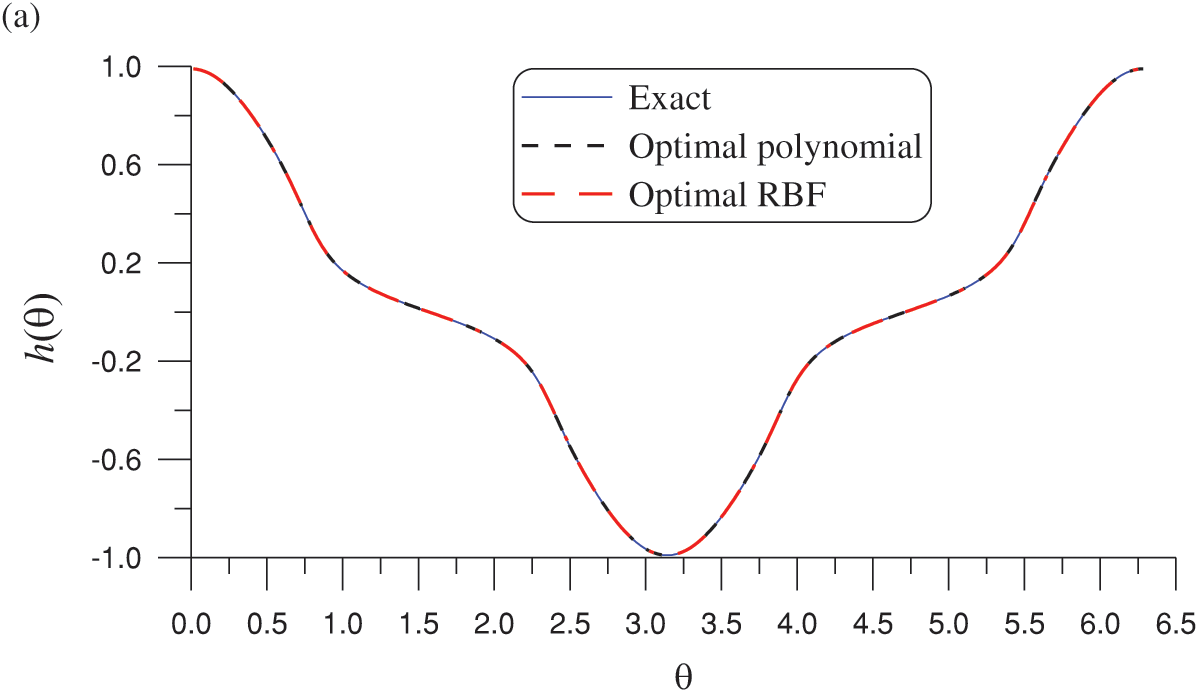
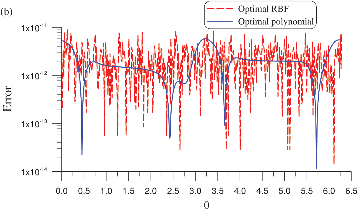
Figure 7: (a) Comparison of the OPM and optimal MQ-RBF numerical solutions with the exact solution on the boundary and (b) absolute errors for a nonpolynomial Laplace equation with a nonharmonic boundary condition and an peanut shape

For the optimal MQ-RBF, we fix n=525 and nb=445 and seek the proper values of c and D in the range [a1,b1]×[a2,b2]=[0.9,1.8]×[3,6]. The optimal values c=1.341 and D=5.006 were obtained after 13 iterations. In this case, the optimal MQ-RBF result is competitive with that of the OPM (Fig. 7); the method achieved ME = 8.98 × 10−12 and RMSE = 3.09 × 10−12 relative to h(x,y)=sin⁡xcos⁡y on Γ.

6  Conclusions

The key achievements of the paper are summarized as follows:

•   By using the MP technique between two vectors, which is equivalent to the minimization in Eq. (5), merit functions were derived for determining the optimal values of the shape factor and fictitious radius in the MQ-RBF.

•   The similarity between the MP and the effective CN techniques was demonstrated.

•   Searching for a minimum in a preferred range was easily performed by using the sample function. Moreover, only a few operations in the GSSAs were required to determine the optimal shape factor and fictitious radius of the source points. The novel idea of inserting a sample function into the merit function is crucial in this technique.

•   The optimal MQ-RBF is equally stable and accurate regardless of whether it is used to solve the Dirichlet, mixed, or Cauchy problems from the Laplace equation.

•   With different boundary values, the optimal MQ-RBF offered different optimal shape factor and optimal fictitious radius parameters at different ranges.

•   The algorithm is more accurate when the regularization diagonal matrix D is used.

•   The optimal MQ-RBF method is much more accurate for solving the benchmark problem than those reported in the literature.

•   A novel OPM was also developed to solve nonharmonic problems with high accuracy.

Acknowledgement: Thank all the authors for their contributions to the paper.

Funding Statement: This work was financially supported by the the National Science and Technology Council (Grant Number: NSTC 112-2221-E239-022).

Author Contributions: The authors confirm contribution to the paper as follows: study conception and design: Chein-Shan Liu, Chung-Lun Kuo, Chih-Wen Chang; data collection: Chein-Shan Liu, Chih-Wen Chang; analysis and interpretation of results: Chein-Shan Liu, Chih-Wen Chang, Chung-Lun Kuo; manuscript writing: Chein-Shan Liu, Chih-Wen Chang; manuscript review and editing: Chein-Shan Liu, Chih-Wen Chang. All authors reviewed the results and approved the final version of the manuscript.

Availability of Data and Materials: Data will be made available on request.

Conflicts of Interest: The authors declare that they have no conflicts of interest to report regarding the present study.

References

1. Franke, R. (1982). Scattered data in terpolation: Tests of some method. Mathematics of Computation, 38, 81–200. https://doi.org/10.1090/S0025-5718-1982-0637296-4 [Google Scholar] [CrossRef]

2. Kansa, E. J. (1990). Multiquadrics—A scattered data approximation scheme with applications to computational fluid-dynamics-II solutions to parabolic, hyperbolic and elliptic partial differential equations. Computers & Athematics with Applications, 19, 147–161. https://doi.org/10.1016/0898-1221(90)90271-K [Google Scholar] [CrossRef]

3. Liu, C. S., Chen, W., Fu, Z. (2016). A multiple-scale MQ-RBF for solving the inverse Cauchy problems in arbitrary plane domain. Engineering Analysis with Boundary Elements, 68, 11–16. https://doi.org/10.1016/j.enganabound.2016.02.011 [Google Scholar] [CrossRef]

4. Rippa, S. (1999). An algorithm for selecting a good value for the parameter c in radial basis function interpolation. Advances in Computational Mathematics, 11, 193–210. https://doi.org/10.1023/A:1018975909870 [Google Scholar] [CrossRef]

5. Bayona, V., Moscoso, M., Kindelan, M. (2011). Optimal constant shape parameter for multiquadric based RBF-FD method. Journal of Computational Physics, 230, 7384–7399. https://doi.org/10.1016/j.jcp.2011.06.005 [Google Scholar] [CrossRef]

6. Cheng, A. H. D. (2012). Multiquadric and its shape parameter—a numerical investigation of error estimate, condition number, and round-off error by arbitrary precision computation. Engineering Analysis with Boundary Elements, 36, 220–239. https://doi.org/10.1016/j.enganabound.2011.07.008 [Google Scholar] [CrossRef]

7. Chen, W., Hong, Y., Lin, J. (2018). The sample solution approach for determination of the optimal shape parameter in the multiquadric function of the Kansa method. Computers & Mathematics with Applications, 75, 2942–2954. https://doi.org/10.1016/j.camwa.2018.01.023 [Google Scholar] [CrossRef]

8. Iurlaro, L., Gherlone, M., Sciuva, M. D. (2014). Energy based approach for shape parameter selection in radial basis functions collocation method. Composite Structures, 107, 70–78. https://doi.org/10.1016/j.compstruct.2013.07.041 [Google Scholar] [CrossRef]

9. Noorizadegan, A., Chen, C. S., Young, D. L., Chen, C. S. (2022). Effective condition number for the selection of the RBF shape parameter with the fictitious point method. Applied Numerical Mathematics, 178, 280–295. https://doi.org/10.1016/j.apnum.2022.04.003 [Google Scholar] [CrossRef]

10. Chen, C. S., Karageorghis, A., Dou, F. (2020). A novel RBF collocation method using fictitious centres. Applied Mathematics Letters, 101, 106069. https://doi.org/10.1016/j.aml.2019.106069 [Google Scholar] [CrossRef]

11. Fasshauer, G. E., Zhang, J. G. (2007). On choosing optimal shape parameters for RBF approximation. Numerical Algorithms, 45, 345–368. https://doi.org/10.1007/s11075-007-9072-8 [Google Scholar] [CrossRef]

12. Chen, C. S., Karageorghis, A., Li, Y. (2016). On choosing the location of the sources in the MFS. Numerical Algorithms, 72, 107–130. https://doi.org/10.1007/s11075-015-0036-0 [Google Scholar] [CrossRef]

13. Chen, C. S., Noorizadegan, A., Young, D. L., Chen, C. S. (2023). On the determination of locating the source points of the MFS using effective condition number. Journal of Computational and Applied Mathematics, 423, 114955. https://doi.org/10.1016/j.cam.2022.114955 [Google Scholar] [CrossRef]

14. Chen, C. S., Noorizadegan, A., Young, D. L., Chen, C. S. (2023). On the selection of a better radial basis function and its shape parameter in interpolation problems. Applied Mathematics and Computation, 442, 127713. https://doi.org/10.1016/j.amc.2022.127713 [Google Scholar] [CrossRef]

15. Shirzadi, M., Dehghan, M., Bastani, A. F. (2012). A trustable shape parameter in the kernel-based collocation method with application to pricing financial options. Engineering Analysis with Boundary Elements, 126, 108–117. https://doi.org/10.1016/j.enganabound.2021.02.005 [Google Scholar] [CrossRef]

16. Liu, C. S. (2023). The meshless solutions of Laplacian non-harmonic and Cauchy problems by developing novel hybrid methods. Engineering Analysis with Boundary Elements, 157, 34–43. https://doi.org/10.1016/j.enganabound.2023.08.034 [Google Scholar] [CrossRef]

17. Liu, C. S., Liu, D. (2018). Optimal shape parameter in the MQ-RBF by minimizing an energy gap functional. Applied Mathematics Letters, 86, 157–165. https://doi.org/10.1016/j.aml.2018.06.031 [Google Scholar] [CrossRef]

18. Liu, C. S., Young, D. L. (2016). A multiple-scale Pascal polynomial for 2D Stokes and inverse Cauchy-Stokes problems. Journal of Computational Physics, 312, 1–13. https://doi.org/10.1016/j.jcp.2016.02.017 [Google Scholar] [CrossRef]

19. Liu, G., Ma, W., Ma, H., Zhu, L. (2018). A multiple-scale higher order polynomial collocation method for 2D and 3D elliptic partial differential equations with variable coefficients. Applied Mathematics and Computation, 331, 430–444. https://doi.org/10.1016/j.amc.2018.03.021 [Google Scholar] [CrossRef]

20. Oruc, Ö. (2019). Numerical solution to the deflection of thin plates using the two-dimensional Berger equation with a meshless method based on multiple-scale Pascal polynomials. Applied Mathematical Modelling, 74, 441–456. https://doi.org/10.1016/j.apm.2019.04.022 [Google Scholar] [CrossRef]

21. Oruc, Ö. (2021). An efficient meshfree method based on Pascal polynomials and multiple-scale approach for numerical solution of 2-D and 3-D second order elliptic interface problems. Journal of Computational Physics, 428, 110070. https://doi.org/10.1016/j.jcp.2020.110070 [Google Scholar] [CrossRef]

22. Oruc, Ö. (2023). A strong-form meshfree computational method for plane elastostatic equations of anisotropic functionally graded materials via multiple-scale Pascal polynomials. Engineering Analysis with Boundary Elements, 146, 132–145. https://doi.org/10.1016/j.enganabound.2022.09.009 [Google Scholar] [CrossRef]

23. Oruc, O. (2023). A local meshfree radial point interpolation method for Berger equation arising in modelling of thin plates. Applied Mathematical Modelling, 122, 555–571. https://doi.org/10.1016/j.apm.2023.03.014 [Google Scholar] [CrossRef]

24. Liu, C. S. (2014). A maximal projection solution of ill-posed linear system in a column subspace, better than the least squares solution. Computers & Mathematics with Applications, 67, 1998–2014. https://doi.org/10.1016/j.camwa.2014.04.011 [Google Scholar] [CrossRef]

25. Koushki, M., Jabbari, E., Ahmadinia, M. (2020). Evaluating RBF methods for solving PDEs using Padua points distribution. Alexandria Engineering Journal, 59, 2999–3018. https://doi.org/10.1016/j.aej.2020.04.047 [Google Scholar] [CrossRef]

26. Tsai, C. H., Kolibal, J., Li, M. (2010). The golden section search algorithm for finding a good shape parameter for meshless collocation methods. Engineering Analysis with Boundary Elements, 34, 738–746. https://doi.org/10.1016/j.enganabound.2010.03.003 [Google Scholar] [CrossRef]

Appendix

In this appendix, we lay out the code in the computer program used to obtain (xkc,xkc):

k=0

Doi=1,m10

θi=2πi/m10

Doj=1,m20

k=k+1

xkc=jD/m20cos⁡θi,ykc=jD/m20sin⁡θi,(A.1)

and the components Gij and bj of G and b in Eq. (11):

Doi=1,m1

θ=2πi/m1

Doj=1,m2−1

xj=jρ(θ)/m2cos⁡θ,yj=jρ(θ)/m2sin⁡θ

K=m2(i−1)+j

bK=0

DoL=1,n

GKL=(xj−xLc)2+(yj−yLc)2+2c2(xj−xLc)2+(yj−yLc)2+c23.

Doi=1,nb

θ=2πi/nb

xj=ρ(θ)cos⁡θ,yj=ρ(θ)sin⁡θ

bK=h(xj,yj)

DoL=1,n

K=m1×(m2−1)+i

GKL=(xj−xLc)2+(yj−yLc)2+c2.(A.2)