
 Submit a Paper
 Propose a Special lssue
 Open Access
ARTICLE

Isogeometric Analysis of Hyperelastic Material Characteristics for Calcified Aortic Valve
1 School of Mechanical Engineering, University of Shanghai for Science and Technology, Shanghai, 200093, China
2 Department of Cardiac Surgery, Zhongshan Hospital, Fudan University, Shanghai, 200093, China
3 School of Mechanical Engineering and Automation, Beihang University, Beijing, 100191, China
* Corresponding Author: Wenshuo Wang. Email:
Computer Modeling in Engineering & Sciences 2024, 139(3), 2773-2806. https://doi.org/10.32604/cmes.2024.046641
Received 09 October 2023; Accepted 25 December 2023; Issue published 11 March 2024
 View Full Text
 Download PDF
Abstract
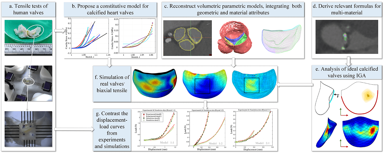
This study explores the implementation of computed tomography (CT) reconstruction and simulation techniques for patient-specific valves, aiming to dissect the mechanical attributes of calcified valves within transcatheter heart valve replacement (TAVR) procedures. In order to facilitate this exploration, it derives pertinent formulas for 3D multi-material isogeometric hyperelastic analysis based on Hounsfield unit (HU) values, thereby unlocking foundational capabilities for isogeometric analysis in calcified aortic valves. A series of uniaxial and biaxial tensile tests is executed to obtain an accurate constitutive model for calcified active valves. To mitigate discretization errors, methodologies for reconstructing volumetric parametric models, integrating both geometric and material attributes, are introduced. Applying these analytical formulas, constitutive models, and precise analytical models to isogeometric analyses of calcified valves, the research ascertains their close alignment with experimental results through the close fit in displacement-stress curves, compellingly validating the accuracy and reliability of the method. This study presents a step-by-step approach to analyzing the mechanical characteristics of patient-specific valves obtained from CT images, holding significant clinical implications and assisting in the selection of treatment strategies and surgical intervention approaches in TAVR procedures.Graphic Abstract
Keywords
Calcific aortic valve disease (CAVD) is a significant cardiac valve pathology, particularly afflicting the elderly population, and ranks as the third most prevalent cause of heart disease, as shown in Fig. 1 [1]. Tongji Medical College in Hubei Province, China, conducted an extensive investigation focusing on individuals aged 60 years and older. Among the analyzed pool of 3,948 samples, a notable 1.93% exhibited severe heart disease, primarily manifesting as aortic insufficiency [2]. The urgency of this issue is underscored by the aging trend in China, with data from the National Health Commission predicting that the elderly population (aged 60 years and above) will surpass 400 million by 2035. Extrapolating from these figures, it is projected that approximately 7.72 million individuals might grapple with aortic insufficiency, consequently imposing a considerable medical burden. This scenario highlights the critical importance of comprehensively and promptly addressing CAVD.
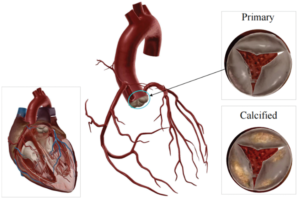
Figure 1: Heart valves
Transcatheter heart valve replacement (TAVR) offers a less invasive alternative for treating valve disorders via peripheral vascular pathways, thereby avoiding sternotomy and the risks associated with cardio-pulmonary circulation. However, selecting the right replacement valve without damaging the native aortic valve and successfully replacing it remains challenging for surgeons. Mu et al. demonstrated that rupture dramatically impacts hemodynamics [3]. Previous investigations involving TAVR patients afflicted with aortic root rupture have conclusively identified the rupture site as a high-stress region [4]. As TAVR demand grows, the computer simulation of patient-specific valve mechanical properties significantly enhances the feasibility assessment of surgical procedures and augments the success rate, also aiding in choosing the size of the replacement valves [5].
In order to achieve a more precise simulation of patient-specific valve mechanical properties, two aspects should be considered: the selection of a constitutive model accurately reflecting the mechanical behavior of the calcified valve and employing a calculation method with high precision and computational efficiency.
Global researchers have extensively explored the constitutive model of heart valves. Noteworthy work in 1995 by May-Newman and Yin exposed mitral valve traits, emphasizing nonlinear hyperelasticity and anisotropy [6]. Li et al. found differing results in leaflet deformations, stress magnitudes, and distributions between isotropic and anisotropic models, with the maximum longitudinal normal stress increased, and the maximum transversal normal stress and in-plane shear stress decreased with the inclusion of anisotropy [7]. In 2005, Sun et al. used a Fung-elastic material model that incorporated material parameters and axes derived from actual leaflet biaxial tests and measured leaflet collagen fiber structure to perform stress-strain analysis of the lobules [8]. Progressing to 2009, May-Newman et al. introduced hyperelastic constitutive equations for aortic valves [9]. Advancements by Sirois et al. in 2011 generalized the Fung-elastic model for fluid simulation of prosthesis valves [10]. In 2012, a Mooney–Rivlin hyperelastic constitutive law was adopted at stent implantation [11,12]. Almost concurrently, based on the fiber-reinforced material model, an anisotropic hyperelastic model was adopted to characterize the mechanical behaviors of aortic tissues [13,14]. In 2014, Wang et al. used the anisotropic hyperelastic Holzapfel–Gasser–Ogden material model to analyze human heart tissues [15]. However, there is no constitutive model that accurately captures the mechanical properties of calcified valves.
Isogeometric analysis, presented by Hughes et al. [16], incorporates the exact geometrical description inherent in a computer-aided design (CAD) model into the analysis by employing the same spline basis functions utilized in the CAD system. Unlike the traditional finite element method, isogeometric analysis (IGA) demonstrates enhanced performance in dealing with nonlinear problems. The use of spline technology ensures a more precise construction of patient-specific valve geometry. High-order precision non-uniform rational B-splines (NURBS) surfaces facilitate effective mesh computation, even under significant deformation. Additionally, IGA obviates the need for repeated mesh refinement during nonlinear analysis, resulting in a substantial reduction in computational time. Furthermore, IGA is proficient in constructing and analyzing models involving dispersive and diffusive multi-materials by assigning material properties to control points [17–19]. Recently, it has gained substantial significance in analyzing the mechanical properties of heart valves [20–24].
Morganti et al. [25] and Xu et al. [20] employed NURBS to extract heart valve geometry from computed tomography (CT) images for model reconstruction. Additionally, in 2015, Kamenskya et al. introduced a geometric flexibility technique for computational fluid-structure coupling (FSI), successfully simulating the dynamic function of a three-valve biological valve throughout the cardiac cycle [23]. In 2017, Takizawa et al. utilized the Space-Time Topology Change (ST-TC) method for moving grid calculations in flow problems, focusing particularly on the inter-leaflet contact of heart valves and preserving high-resolution representation near the blade surface while effectively addressing contact regions [26]. In 2019, Bianchi conducted patient-specific aortic reconstruction using NURBS splines [27]. Building on these advancements, Zhang et al. in 2021, presented an effective computational analysis framework for simulating primary and replacement three-leaf heart valves based on isogeometric analysis [28]. Concurrently, Johnson et al. established a parameter-based approach for modeling tricuspid valves in a utility program, providing a robust and versatile method for assessing the performance and efficiency of various leaflets through isogeometric analysis [29].
Although extensive research has been conducted on the mechanical attributes of heart valves, certain issues persist. Initially, valve materials are often oversimplified, adopting isotropic linear characteristics or described using classical constitutive models [13,30]. Subsequently, the lack of consideration for valve thickening at calcification sites results in an ideal model with uniform thickness, significantly diverging from authentic valve morphology. Moreover, the precise extent and distribution of valve calcification remain inadequately captured. To address these issues, this paper proposes a method for studying the mechanical characteristics of patient-specific heart valves using CT images, aiming to maintain model authenticity and enhance the accuracy of valve mechanical analysis. The key contributions of this paper are outlined as follows:
1. The pertinent formulas for 3D multi-material isogeometric hyperelastic analysis based on Hounsfield unit (HU) values are derived, enabling the foundational capabilities of isogeometric analysis for calcified aortic valves. The feasibility of these formulas is verified by the analysis results of ideal heart valves.
2. Various constitutive models are fitted to accurately capture the stress-strain behavior of calcified heart valves via a range of uniaxial, equiaxial, and non-equiaxial experiments on human calcified valves. The best-performing model is chosen based on its fitting results, and its accuracy is confirmed through experimental comparisons.
3. Aortic valve models with patient-specific material distribution are created from CT images using NURBS splines to build accurate volume parametric models for isogeometric analysis. This approach addresses challenges such as high computational costs, convergence difficulties, and mesh distortions commonly encountered in traditional dense mesh methods.
4. The fitting quality of the displacement-load diagrams obtained from biaxial tensile tests on heart valves is compared with the displacement-load diagrams from the experimental simulation results of the reconstructed valves, validating the feasibility and accuracy of the methods and procedures employed in this study.
The structure of this paper is as follows: Section 2 presents the derivation of basic formulas for 3D isogeometric hyperelastic analysis. Section 3 details the fitting process of constitutive equations. Section 4 presents the valve CT reconstruction procedure, accompanied by numerical examples and validation of the proposed method through real valve simulations. The outcomes and significance of the findings are elucidated in Section 5. Section 6 summarizes the conclusions and future works.
2 Basic Formulas of Isogeometric Hyperelastic
2.1 Basic Theories of Isogeometric Analysis
Current CAD systems usually use NURBS for geometric representation and use basis functions instead of shape functions of finite elements. The
where
With the definition of the B-spline basis function, a 3D NURBS patch can be defined by three-knot vectors with the following expressions:
where
where
2.2 Isogeometric Hyperelastic Numerical Formula
In a nonlinear system, the deformation gradient
where
Meanwhile, the Lagrangian strain
Thereafter, the three-dimensional Lagrange strain variation can be derived as follows:
with
where
Then, the increment of the three-dimensional Lagrange strain can be defined as follows:
The relationship between the variation and increment of the second Piola–Kirchhoff stress
where
The strain energy can be defined as follows:
Thereafter, strain energy variation can be derived as follows:
Since nonlinear equations cannot be solved directly, they can be iteratively solved using the Newton-Raphson method. To find the displacement increment, one must linearize the weak form of the governing equation.
with
2.3 Multi-Materials Realization Based on Hu Value
2.3.1 Strain Energy Density Function
When a material state can be entirely described by a given total strain, it is termed hyperelasticity. For hyperelastic materials, the stored strain energy remains constant as long as the strain within the material is constant, as demonstrated in Fig. 2. Consequently, the strain energy density function emerges as the optimal choice for analyzing hyperelastic material models. In such materials, the strain energy density exists as a function of strain, allowing stress to be derived through differentiation [32,35].
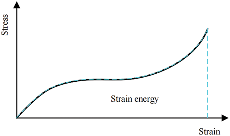
Figure 2: Stress-strain relationship of hyperelastic material
Since the invariant does not vary with the reference coordinate system, regardless of the loading conditions an object undergoes, the strain energy density can be defined using the invariants of strain or alternatively, those of the deformation tensor. The three invariants of the right Cauchy–Green deformation tensor
where the square root of
Incompressibility in materials can lead to numerous challenges in constitutive relations, particularly when combined with nonlinearities such as large displacements, large strains, and contact. In order to separate the distortion part from dilatation, it is necessary to introduce the so-called reduced invariants
Several typical hyperelastic models are listed in Table A1 of the Appendix.
The nominal stress (first Piola-Kirchhoff stress) in the direction of stretch is obtained by differentiating the strain energy density with respect to the principal stretch as follows:
Moreover, the second Piola-Kirchhoff stress is calculated by differentiating the strain energy density with respect to the Lagrangian strain:
The Mooney-Rivlin model, frequently utilized as a strain energy density function, facilitates the specific solving process of the second Piola-Kirchhoff stress
Furthermore, the two-parameter strain energy density function of the Mooney-Rivlin model, including the incompressibility coefficient, is defined as
The second Piola-Kirchhoff stress
which can be rewritten as
with
where the subscribed comma denotes derivative, i.e.,
Based on Eq. (14), the tangent constitutive tensor
with
The formulas for the second Piola-Kirchhoff stress
Mimics integrates both intuitive manual tools and fully automated algorithms for knee joint and cardiac segmentation, aiding medical practitioners in accurately processing patients’ medical images. During calcified region annotation via thresholding in Mimics, the
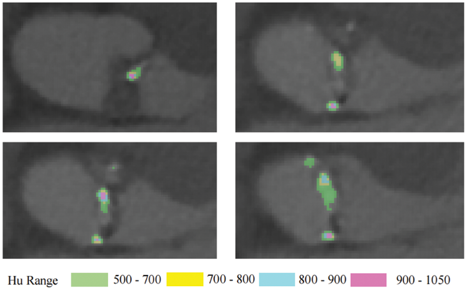
Figure 3: The distribution of
Therefore, treating individual calcified regions of the valve as the same material results in relatively weak accuracy. Isogeometric analysis methods inherently offer advantages in multi-material model analysis. Material properties are assigned to various control points, and continuous refinement of the calcified regions allows the simulation to progressively approximate the real calcification scenario.
This study only considers hyperelastic materials, and the material properties at control points are defined based on the gray value
where
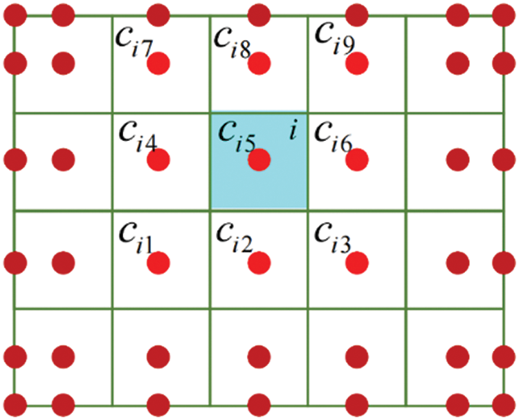
Figure 4: The relationship of element and control points
Thus, the second Piola-Kirchhoff stress
3 Constitutive Model Experiment
Existing research on heart valve mechanical properties often utilizes fresh pig, cow, donkey, and other mammalian valve tissues for experimental testing [38,39]. However, due to these animals’ shorter lifespans, their aortic valve tissue rarely undergoes calcification, making it less suitable for this study. The heart valve tissue utilized in our experiment was provided by the Department of Cardiac Surgery at Zhongshan Hospital, affiliated with Fudan University. Previous studies have shown that valve tissue’s mechanical properties can be preserved at low temperatures [40]. Obtaining human valve samples is challenging, so the valves used in this study were refrigerated prior to batch testing. The degree of calcification in heart valves can be categorized into three types [41,42]: Fig. 5a shows mild calcification; Fig. 5b moderate calcification; Fig. 5c severe calcification. Severe calcification, which makes the valve material akin to linear material and significantly stiffer than native valves, is unsuitable for TAVR surgery and, thus, of limited significance in this study. Instead, the primary focus is on cases of mild and moderate calcification.
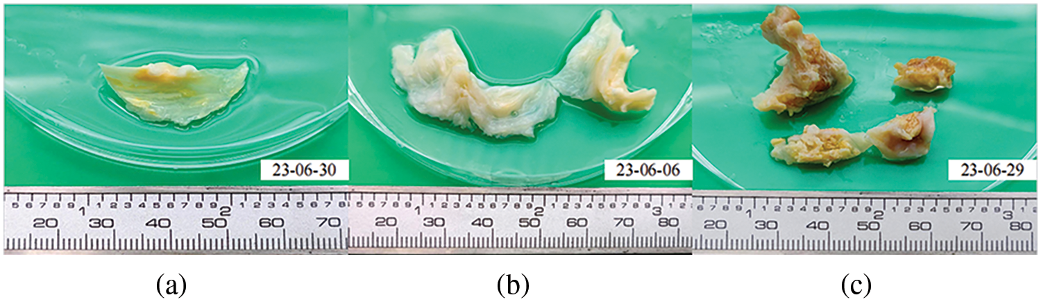
Figure 5: Calcified heart valves
Biaxial stretching experiments provide a more precise characterization of mechanical properties than uniaxial stretching [43]. May-Newman et al. have extensively described biaxial mechanical testing methods for valve leaflet tissues [44,45], forming the basis of this study. Additionally, early research discovered the anisotropic behavior and collagen fiber structure of aortic valve tissue. Stiffness is higher parallel to collagen fibers and lower in the transverse direction. Therefore, distinguishing between the circumferential and radial directions of the valve is essential during experiments.
The experimental instrument employed in this study is the CellScale Biotester biaxial testing system, as illustrated in Fig. 6. This system, specifically designed for biological materials, features a comprehensive biaxial testing setup. Its sample clamps, made of tungsten alloy and electrochemically sharpened, facilitate easy penetration of sample structures. Moreover, the system maintains the biological activity of samples by providing temperature-controlled water bath conditions during experiments.
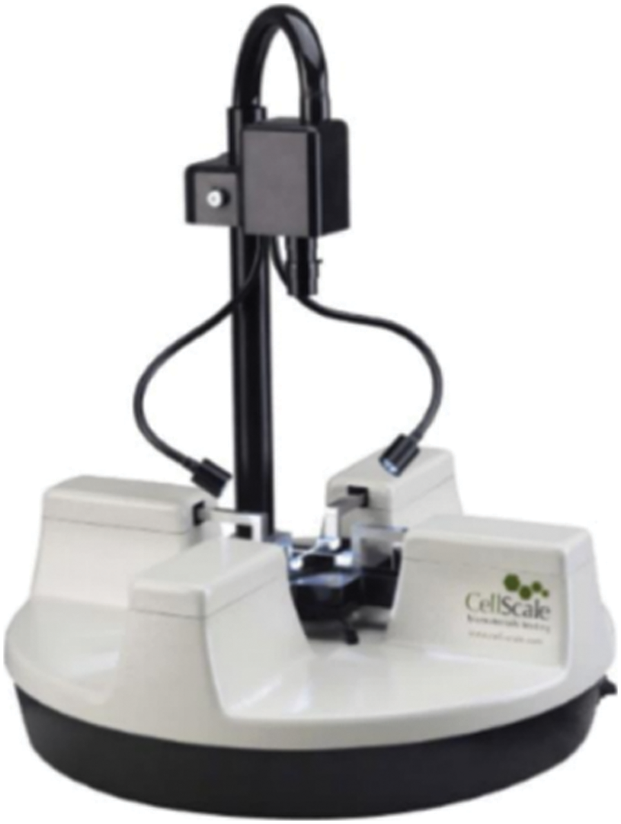
Figure 6: CellScale Biotester
Given the smaller size of human valves compared to those of other animals such as pigs and cows, and considering the susceptibility of calcified valve leaflets to tearing and delamination during stretching, the researchers decided not to trim the valves in the biaxial experiments. The overall experimental procedure is outlined below:
1. Before clamping the samples, a vernier caliper was used to measure the thickness of the leaflet in the central plane area ten times. The average of these measurements was then taken as the overall sample thickness for subsequent stress calculations.
2. Using the measured thickness plane area from Step 1 as the clamping center, marking points were positioned at the sample’s center using carbon powder or ink for real-time displacement tracking during software processing.
3. The sample was placed on the clamping fixture board, aligning its circumferential (Circ) and radial (Rad) directions with the main axes of the biaxial testing system.
4. The distance between the dual suture hooks was adjusted to 7.5 mm × 7.5 mm, and physiological saline was injected into the water bath tank.
5. The sample was clamped onto the biaxial testing system, and the lifting mechanism was lowered to submerge the sample in the water environment. Fig. 7 illustrates the sample clamping setup.
6. Loading distances were set in both the axial and radial directions for equiaxial and non-equiaxial stretching experiments. In equiaxial stretching experiments, the axial and radial step distances were identical, i.e., 1:1. In non-equiaxial stretching experiments, the axial and radial step distances differed, i.e., 1:2 and 2:1.
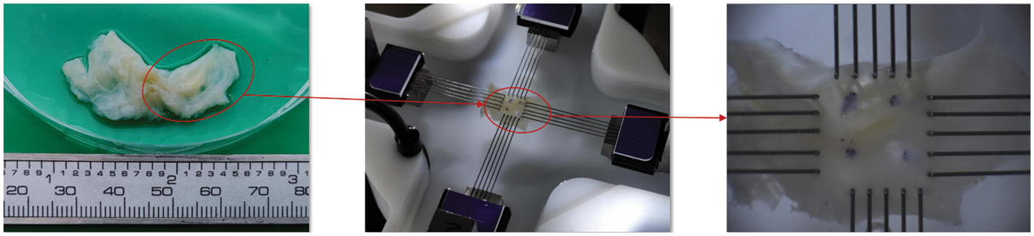
Figure 7: Biaxial tensile sample preparation and clamping
Due to the reliance on the quality of carbon powder and ink marks for marker point displacement tracking, this study employs a quality filtering process to minimize the influence of this error. A square region at the center of the clamping area is divided, containing 30 mm × 30 mm marker points within it. The coordinates at time 0 s are considered the initial coordinates, and the coordinates at each moment during stretching are used as the final coordinates. Fig. 8 shows the trajectories of the marker points, with red points denoting the marker points and white curves representing their trajectories. It can be observed that marker points with clear ink marks exhibit smaller trajectory fluctuations.
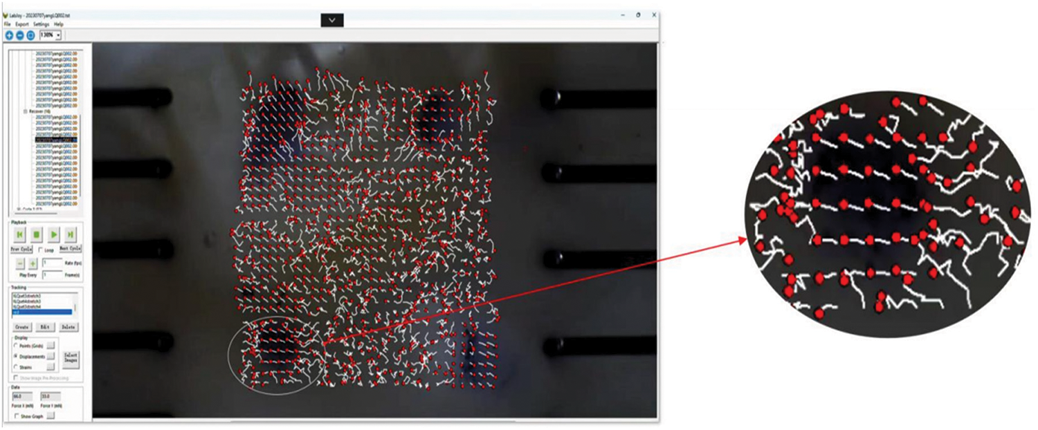
Figure 8: Movement trajectory of the mark point
In order to select marker points with better trajectory detection quality, this study calculates the slope of the line connecting the end and start coordinates of each marker point at each moment. If the sum of the slope deviations does not exceed a predetermined error value, the point is deemed to have good trajectory detection quality. The distance between the marked points in the circumferential and radial directions is calculated using the Euclidean distance formula, as depicted in Fig. 9.
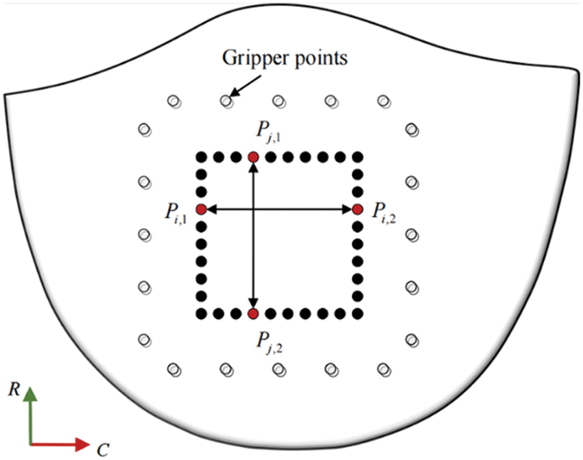
Figure 9: Sample marking points
Assuming the sample holding area resembles a rectangular shape, and
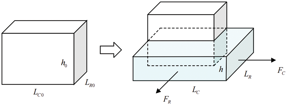
Figure 10: Schematic diagram before and after sample deformation
Cauchy stress on circumferential:
Cauchy stress on radial:
Stretch (Tensile ratio):
Green-Lagrangian strain:
Fig. 11a illustrates the tensile ratio-stress curves of various samples during equiaxial stretching. The curves of the same color depict the response under circumferential and radial stretching conditions for each stretching degree.
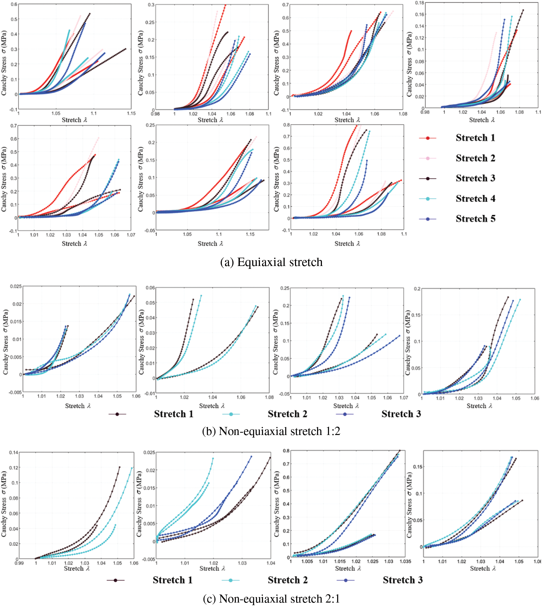
Figure 11: Cauchy stress-stretch curves of biaxial stretch
Figs. 11b and 11c show the tensile ratio-stress curves of various samples during non-equiaxial stretching. The curves of the same color represent the response under circumferential and radial stretching conditions for each stretching degree.
The implementation of strain energy functions in modeling the material properties of soft tissues has demonstrated significant success in biomechanics. The coefficients of the constitutive model, shown in Table A2 of the Appendix, are intricately linked to the strain energy density function, which is unique to the material under consideration. Among the most widely adopted energy density functions used to capture the nonlinear behavior of soft tissue is the Fung strain energy density function, which has proven effective in characterizing the behavior of heart, artery, and mitral valve tissues [46,47]. Despite the progress made, it is worth noting that, to date, no constitutive model has precisely captured the complex stress-strain relationship exhibited by heart valves.
This study employs five representative constitutive equations: the Mooney-Rivlin 9-parameter, Yeoh, Ogden, Fung, and May-Newman models. Nonlinear least squares fitting codes were developed to fit these constitutive models. Experimental data from equiaxial and non-equiaxial tests were fitted with these equations, and the best-fitting model was selected for simulating valve mechanical characteristics. Fig. 12 displays a portion of the experimental data and the effect of curve fitting.
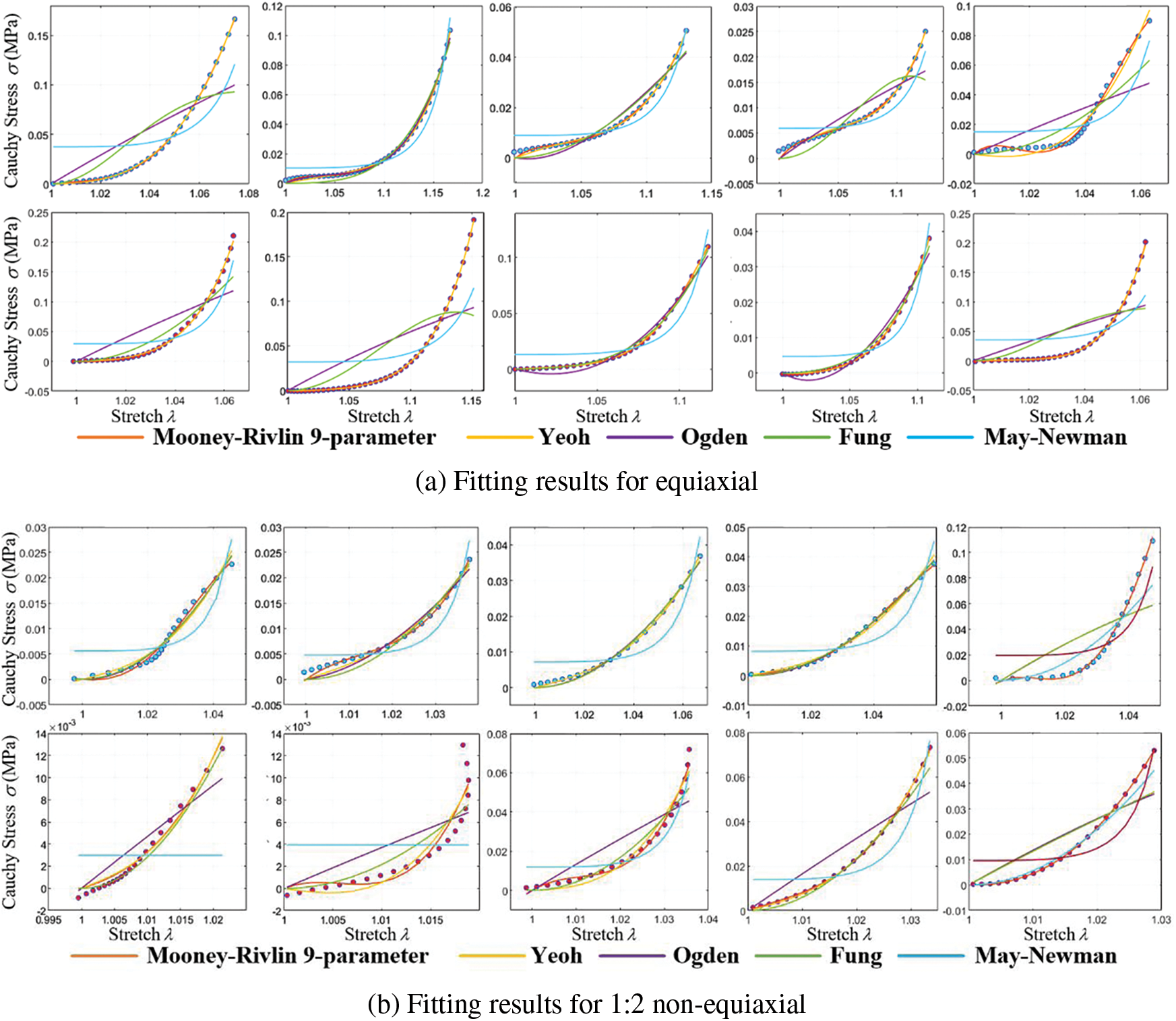
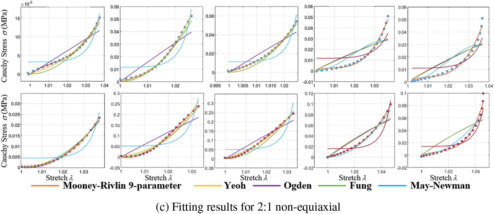
Figure 12: Cauchy stress-stretch curves of biaxial stretch
Curve fitting errors of tensile experimental data under different models are presented in Table 1.

Curve fitting errors, compared in Table 1, reveal that the Mooney-Rivlin 9-parameter model and the Yeoh model exhibit the best fitting performance, accurately representing the stress-strain relationship of calcified heart valve leaflets. Variations may exist among different heart valve tissues and even within the same type of valve tissue among various individuals. The complexity of the model should be carefully balanced, considering the available data and computational resources, to avoid overfitting and excessive parameterization. Due to the higher number of coefficients required for the Mooney-Rivlin 9-parameter model and the similar fitting errors of both models under different stretching conditions, the Yeoh model is chosen for simulating the mechanical characteristics of calcified heart valve leaflets in this study.
Yeoh [48] initially proposed the Yeoh model in 1993. It is a polynomial hyperelastic constitutive model that utilizes polynomial expansion to fit the stress-strain relationship of materials, expressed in the following general form:
where
Fig. 13 depicts the fitting results of various experimental data using the fixed Yeoh model. As the biaxial stretching experiments did not precisely align with the fiber orientation, some associated errors might be present in the experimental outcomes. Nevertheless, the fitting performance indicates satisfactory alignment with circumferential stretching.
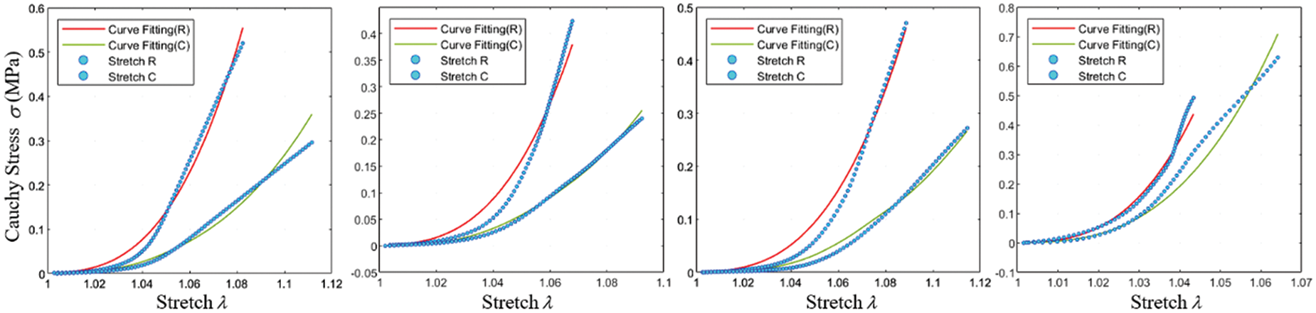
Figure 13: Fitting effect of the constitutive model
The uniaxial tensile test, a common method for measuring the mechanical properties of heart valves [49], was used in this study. Aortic valves with pronounced calcification areas and clear distribution directions were selected for uniaxial stretching experiments. In order to ensure accurate representation, each semilunar valve was meticulously sampled, with one sample taken from each.
The uniaxial tensile experiments were conducted using a YG026G multifunctional electronic fabric strength tester. During sample clamping, the edges were wrapped with gauze to prevent sample slippage. The clamping direction followed the direction of valve calcification to avoid tearing at the junction between the native and calcified valve during stretching. The clamping length was set to10 mm, based on the available sample area, as shown in Fig. 14.
Figure 14: Uniaxial tensile sample preparation and clamping
A force termination target of
Cauchy stress:
Stretch (Tensile ratio):
Green-Lagrangian strain:
The study reveals that severe calcification of the valve leads to higher stiffness and a tendency toward a linear stress-strain relationship. This trend is further illustrated in Fig. 15a, where the stress-strain curve tends to become linear beyond a certain tensile extent. To more accurately determine the constitutive model coefficients of the calcified valve through uniaxial tensile testing, both the original and fully calcified valve segments were subjected to separate tensile tests. The Yeoh model was employed for curve fitting. The outcomes for these two extreme cases are depicted in Figs. 15b and 15c, and the corresponding constitutive model coefficients are presented in Table 2.
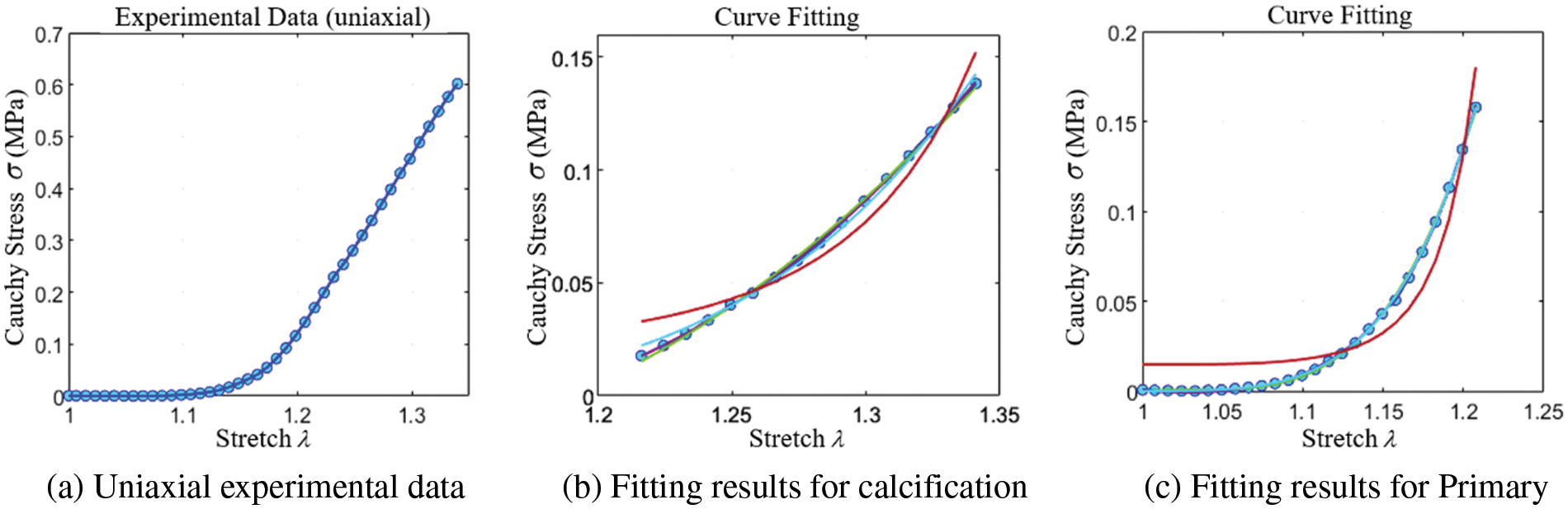
Figure 15: Uniaxial stretch

4.1 CTA Image Model Reconstruction
Due to the significant variations in calcified leaflet properties, especially regarding thickness, it is challenging to describe the leaflet model using a limited set of parameters. Utilizing patient-specific clinical imaging data for reconstruction, the models offer robust support for the accuracy of mechanical calculations and analysis.
Image Data Import and Orientation Adjustment:
The initial step involved importing the patient’s CT scan outcomes in DICOM format into Mimics. Subsequently, precise adjustments were made to ensure that the orientation of the view aligned perpendicularly with the aortic cross-section.
Segmentation of Aortic Valve Root Area:
Segmentation of the aortic valve root area, including both the native valve and the calcified region, was performed based on the variation in
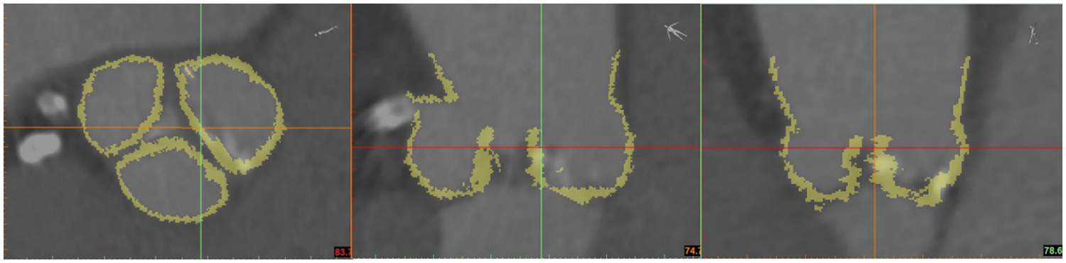
Figure 16: Threshold segmentation
Triangular Mesh Generation and Material Data Derivation:
A triangular mesh model of the aortic valve root area was generated through 3D reconstruction. Additionally,
Leaflets Cutting and Smoothing:
The reverse engineering software Geomagic Wrap was employed to trim and smooth the triangular mesh model of the aortic valve leaflets, as depicted in Fig. 17.
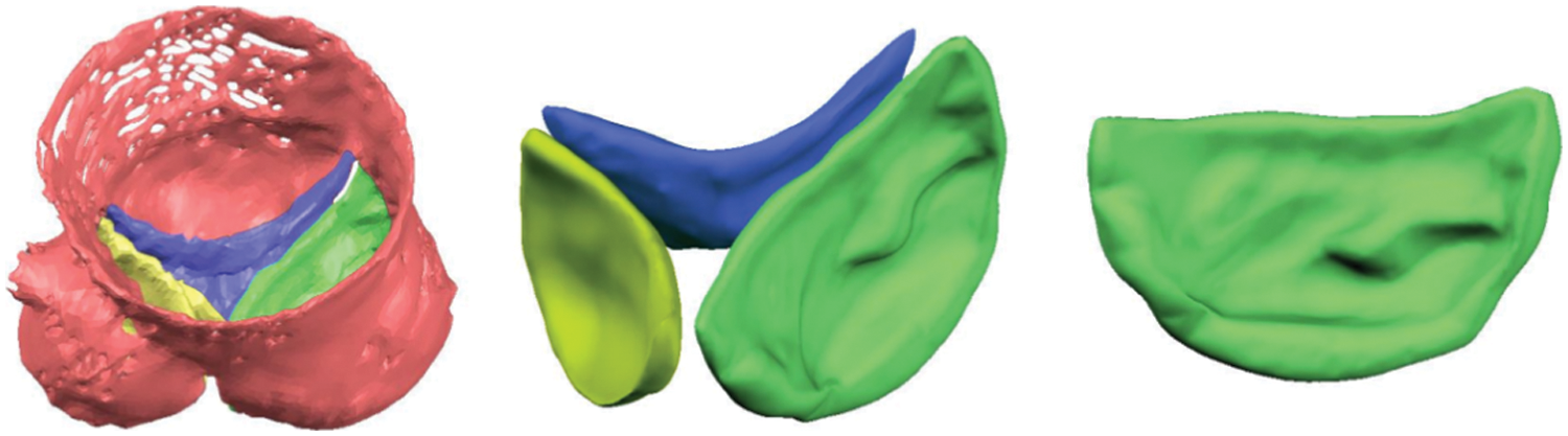
Figure 17: 3D reconstruction and processing
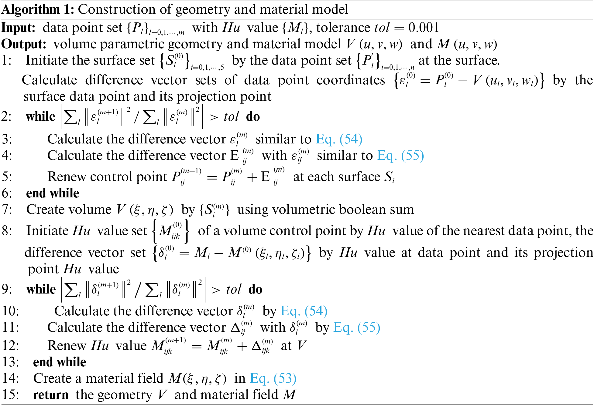
Upon completing the triangular mesh processing, the volume parametric geometry model of the aortic valve leaflet was created utilizing NURBS splines. Initially, the vertices of leaflets triangular mesh, also known as data points
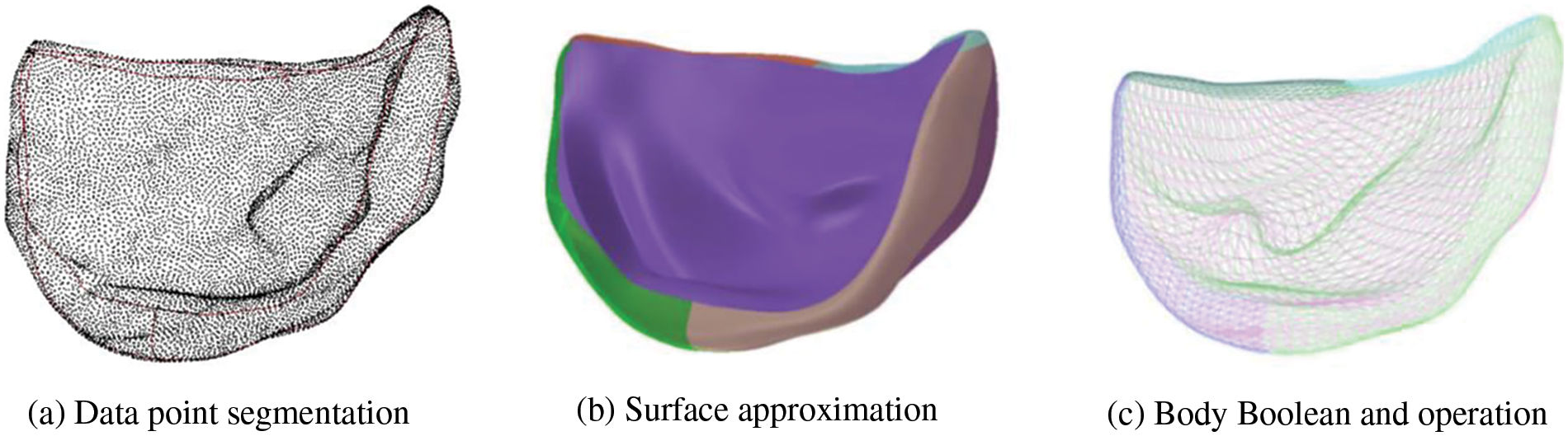
Figure 18: Construction of volume parametric model
When constructing the patient-specific model, both the material model and the geometry model are equally important. The material field
At
The difference vector
where
4.2 Algorithm for Nonlinear Solving
Fig. 19 displays the flowcharts of the source code for linear and nonlinear analyses, differing notably in the resolution of unknown variables.
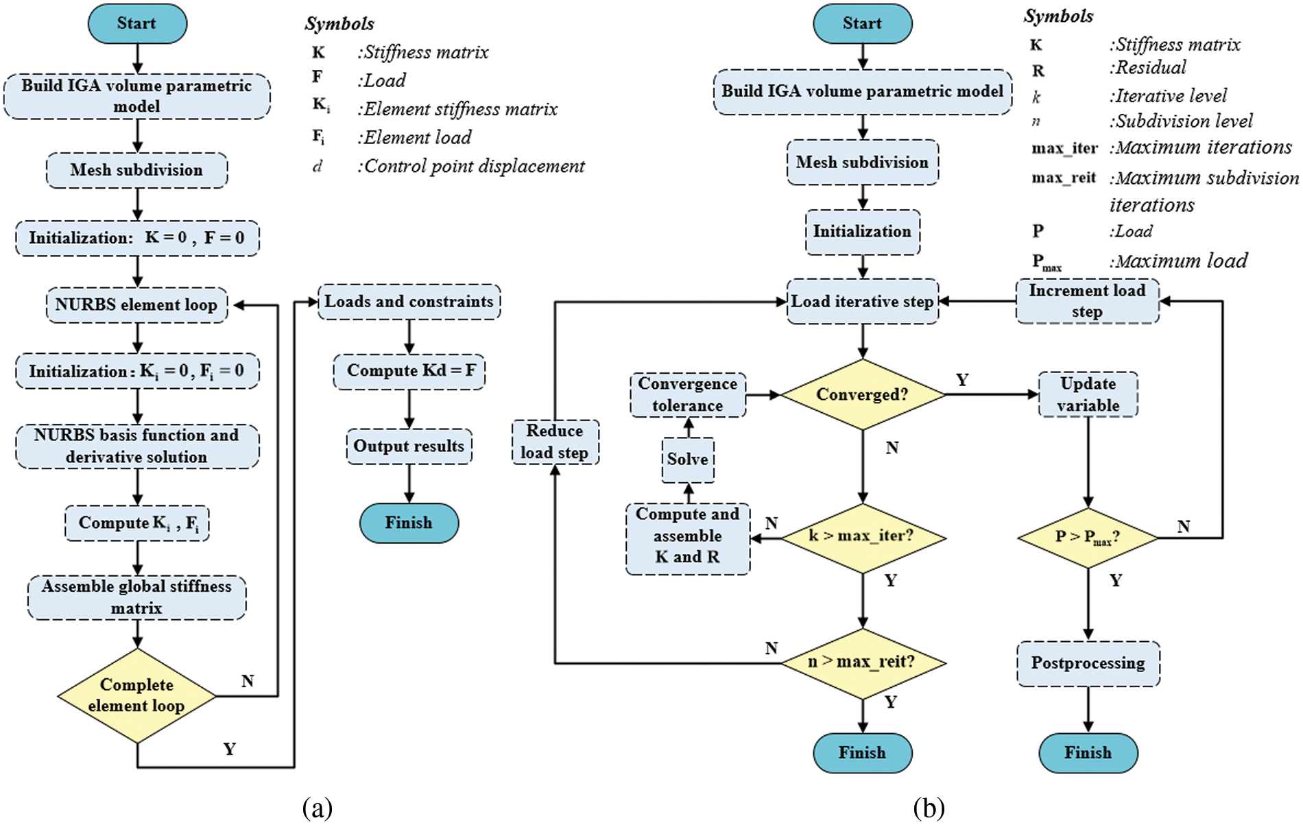
Figure 19: Source code flowchart
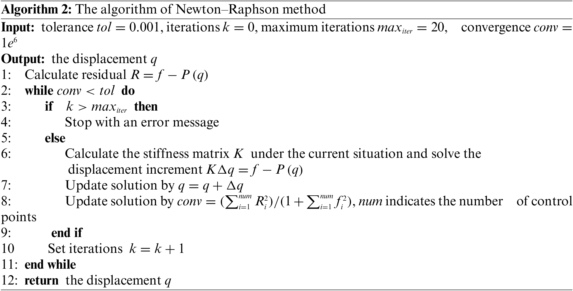
Nonlinear equations cannot be effectively solved using direct methods to achieve a relatively precise solution. This study adopts an automatic load increment approach similar to that in ABAQUS [52], employing the Newton-Raphson method to resolve nonlinear equations. The procedure is detailed in Algorithm 2.
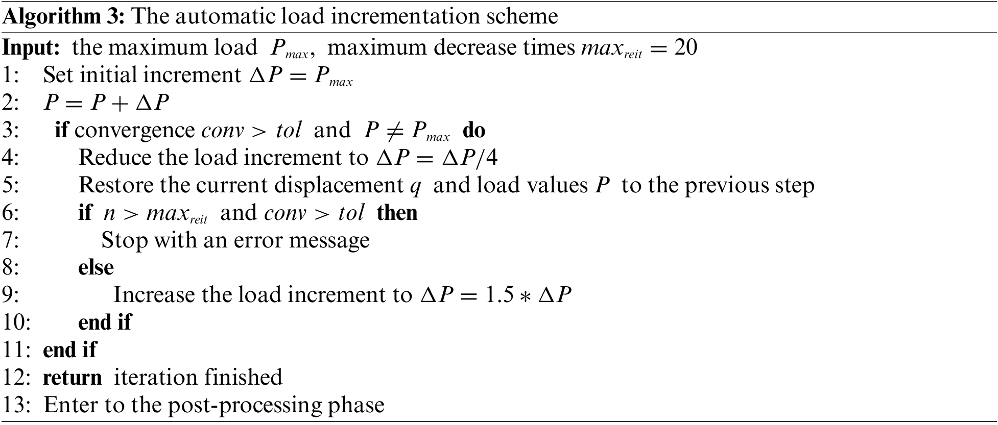
The automatic load incrementation scheme is given in Algorithm 3.
In order to prove the correctness of the method in this study, two hyperelastic models are simulated by an isogeometric analysis program.
1. The model is a square plate with a thickness much smaller than its side length. As shown in Fig. 20a, the length and width of the model are 10 mm, and the thickness is 0.2 mm. Constraints are applied to the lower surface, front surface, and left surface of the plate. The right and back surfaces of the plate are given a prescribed horizontal displacement
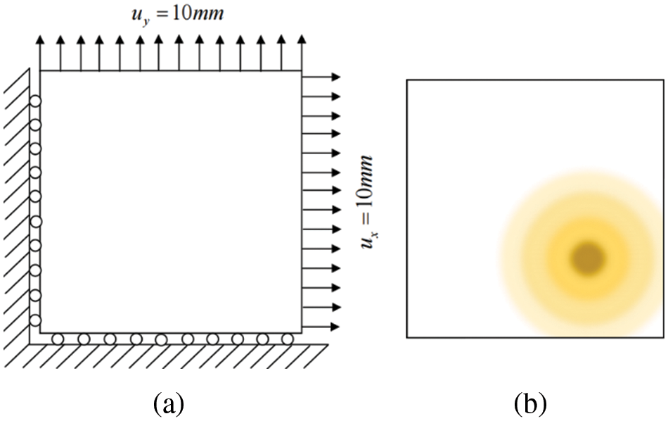
Figure 20: Model constraint
Material 1:
Material 2:
In order to verify the accuracy of isogeometric analysis in hyperelastic materials more accurately, two cases are considered: for a single material, results from both FEA and IGA 3D analyses are displayed in Figs. 21a, 21b, 21d, and 21e. For multiple materials, IGA 3D analysis results are depicted in Figs. 21c and 21f.
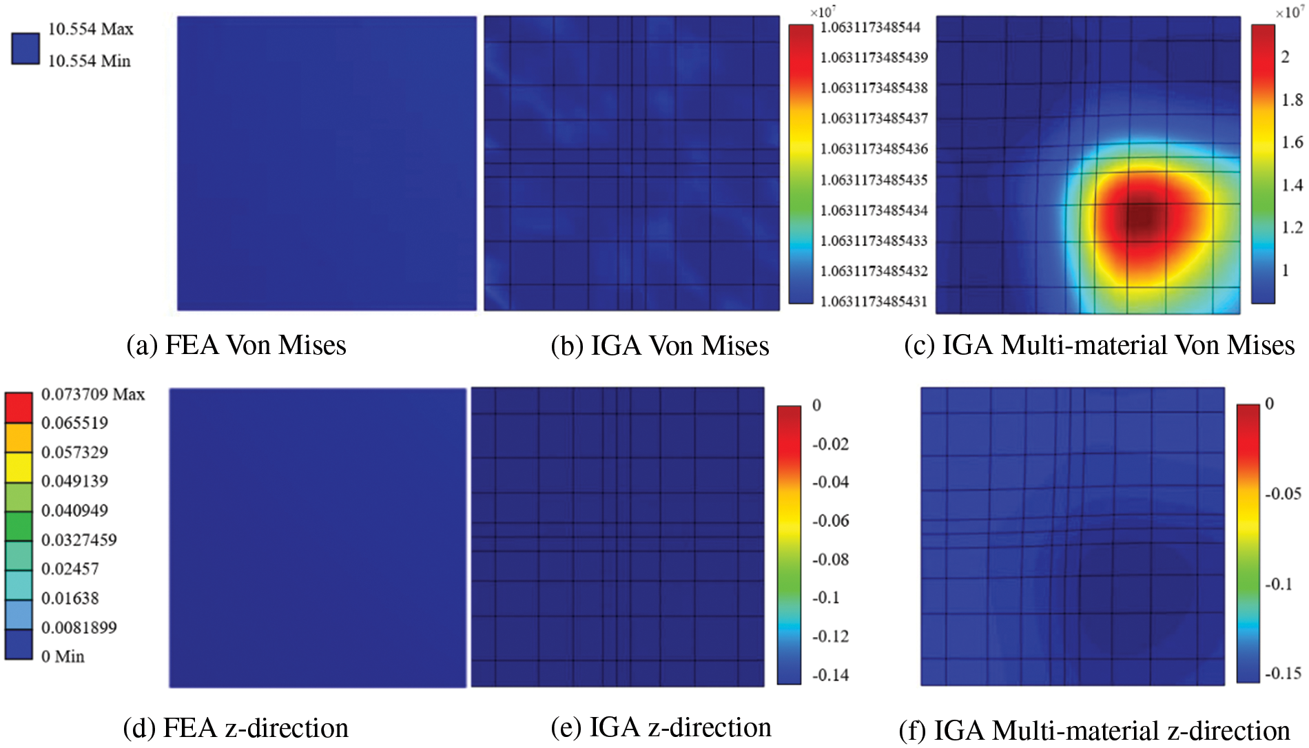
Figure 21: Model analysis results
2. The model represents a leaflet of an ideal aortic valve. A fixed constraint is applied at the junction of the coronary valve and the aorta (valve ring), marked in red in Fig. 22b, and a displacement constraint is applied at the center of the free edge of the coronary valve, marked in blue in Fig. 22a. Fig. 22c illustrates the model’s calcification. The material parameters are set as follows:
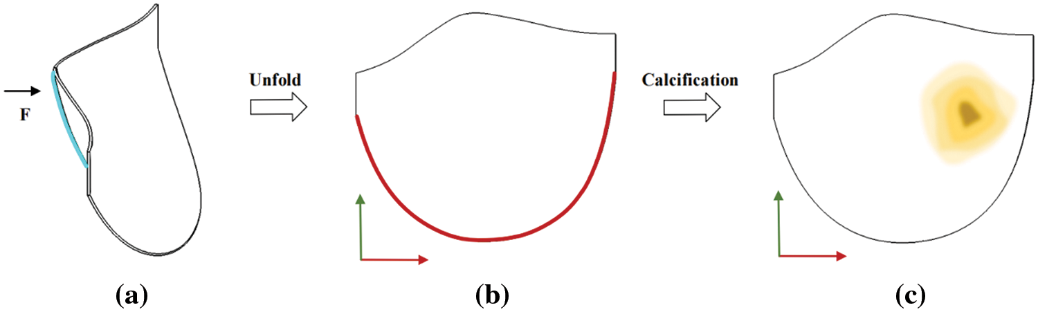
Figure 22: Model constraint and calcification region map
Material 1:
Material 2:
The Von Mises diagram for IGA analysis without calcification is shown in Fig. 23a and with calcification in Fig. 23b. The stress distribution in the x-direction of IGA analysis without calcification is depicted in Fig. 24a and with calcification in Fig. 24b. Fig. 25a displays the displacement distribution in the z-direction of IGA analysis without calcification, while Fig. 25b shows this distribution in the case of calcification. The stress and displacement distribution in both calcified and non-calcified models demonstrate a consistent overall trend. However, in calcified valve regions, a distinct stress concentration pattern is observed, corresponding to actual mechanical analysis.
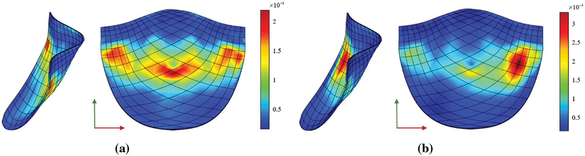
Figure 23: Von Mises
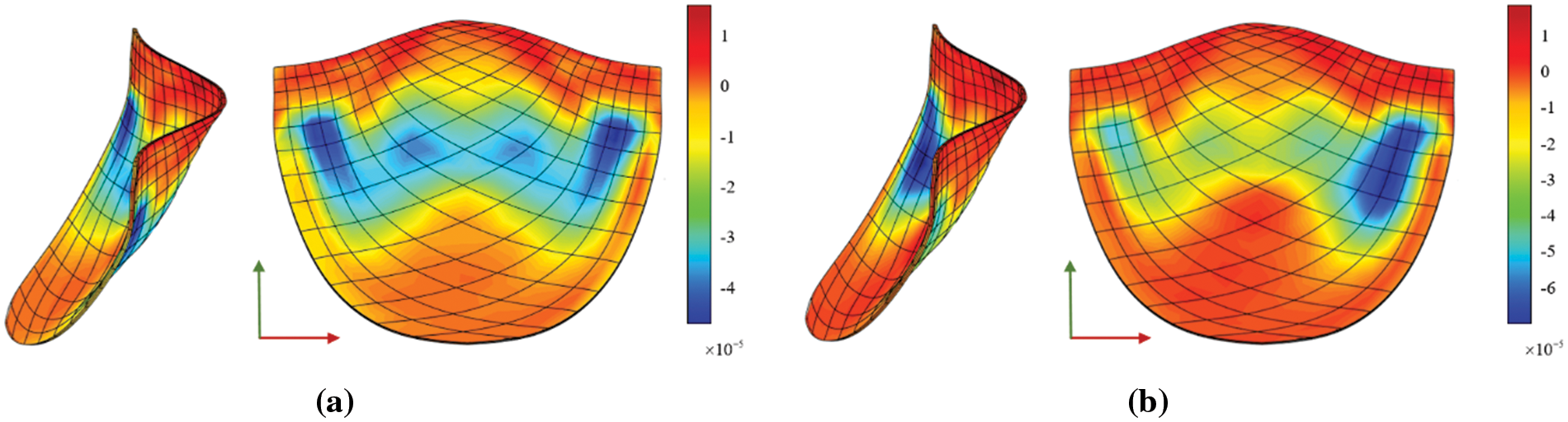
Figure 24: x-direction stress
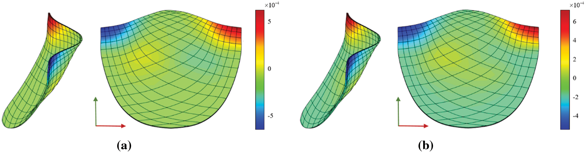
Figure 25: z-direction displacement
When comparing the analysis results of a non-calcified square plate in FEA and IGA, similarities in stress-displacement distribution are apparent. The maximum and minimum values fall within a specific error range, confirming the effectiveness of stress analysis for a basic hyperelastic model in this study. Moreover, these two simulation examples reveal that
4.4 Analysis and Comparison of Mechanical Properties of Valve
Considering that valve CT data is scanned while the valve is operational, the reconstructed valve shape may deviate from its form under experimental conditions. In order to facilitate a comprehensive comparison between the experiment and simulation during biaxial valve stretching, the simulation valve model is meticulously adjusted to closely emulate the experimental valve’s configuration. This involves a procedure to flatten the valve before conducting model analysis and fine-tuning the valve’s orientation to align the circumferential and radial directions parallel to the corresponding coordinate axes, as illustrated in Fig. 26.
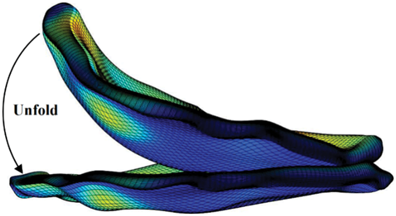
Figure 26: Valve unfold diagram
A square with a side length of 6.7 mm is formed around the restraint and loading ends in the circumferential and radial directions of the valve. The specific constraints and loading modes are shown in Fig. 27. The two adjacent sides of the valve are fixed, and the other two sides are subjected to displacement constraints.
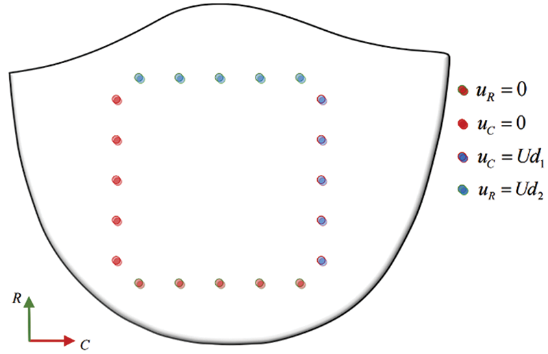
Figure 27: Model constraint and load
The following figures display the biaxial tensile simulation results of the valve under varying calcification conditions. Figs. 28a–28c exhibit the calcification of one leaflet in each of the three patients. The color bar on the right represents the
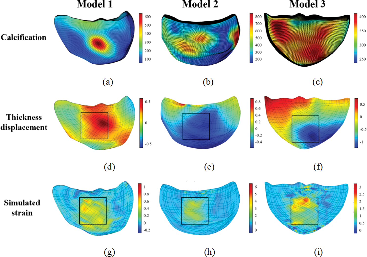
Figure 28: Biaxial tensile simulation results of the valves
In Section 2.3, the strain energy density function is fitted to the stress-strain curve obtained from processing experimental data, resulting in the best-fit constitutive model and model coefficients. This model is then applied to simulate the valve reconstruction model in Section 3.1, replicating the valve’s biaxial tensile test. The simulation produces a displacement-load curve, which is compared with the actual experimental results. The curve’s conformity analysis verifies the simulation approach used in this study and indirectly corroborates the appropriateness of the selected constitutive model, as outlined in Section 2.3. The specific comparison process is shown in Fig. 29.
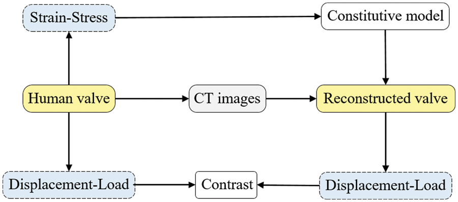
Figure 29: Comparison flow chart
Considering the significantly greater stiffness of the calcified region of the valve compared to the non-calcified region, it is imperative in the simulation to position the maximum load point at the calcification center. Concurrently, displacement measurements should be recorded at the clamping edge proximal to this center, as delineated in Fig. 30.
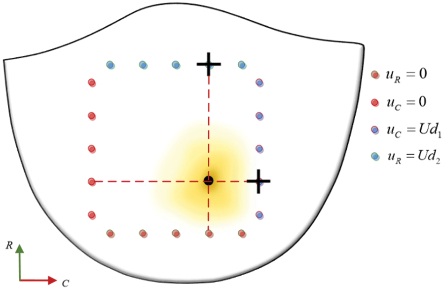
Figure 30: Contrast data selection
The displacement-load curves derived from various experimental samples at differing stretching ratios were juxtaposed with those procured from the simulation, as shown in Fig. 31.
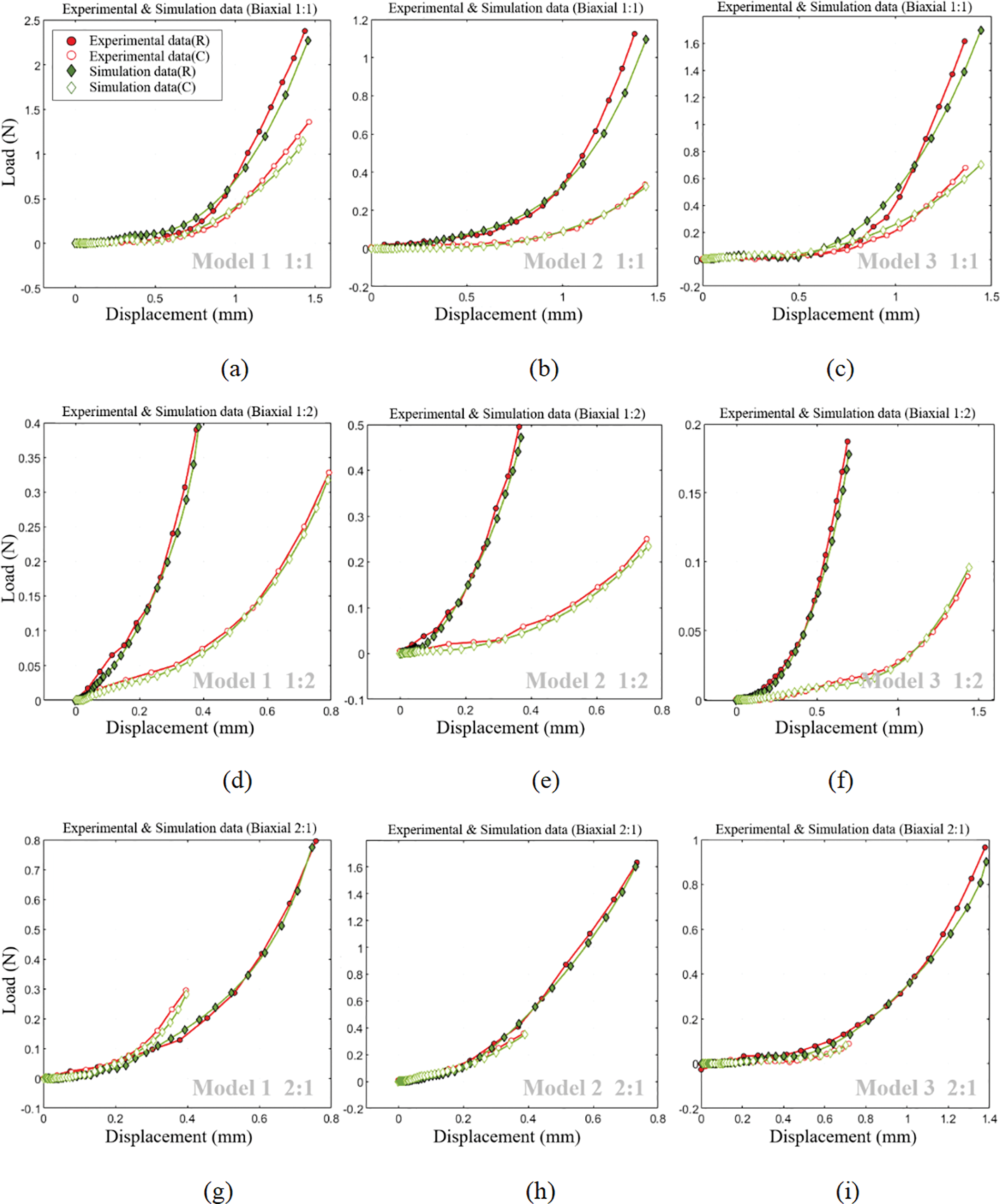
Figure 31: Comparison of experimental and simulation displacement-load curves
Fig. 28 reveals that within the stretching region, the valve’s strain and displacement distribution closely mirrors the actual calcified area. Furthermore, as depicted in Fig. 31, a noteworthy congruence exists between displacement-load curves from both biaxial stretching simulations and experimental data. This congruence not only affirms the simulation method’s relevance but also indirectly validates the accuracy of the selected constitutive model in replicating the valve’s mechanical characteristics.
In this investigation, a thorough analysis was conducted on the mechanical properties of patient-specific calcified valves using CT imaging, thereby introducing an innovative perspective into the feasibility of TAVR surgery.
Constitutive Model Fitting: The comparison between equiaxial and non-equiaxial stretching scenarios reveals the fitting errors of various classical constitutive models to experimental data. Notably, the Yeoh model exhibited the smallest fitting error, indicating its superior ability to express the strain energy density function of calcified valves. The favorable fitting results of the Yeoh model, as shown in Fig. 13, provide empirical evidence supporting the model’s validity.
Multi-material based on Hu value: The square plate model’s analytical outcomes indicate congruent stress-strain distributions under biaxial stretching conditions, validating the correctness of the derived three-dimensional isogeometric hyperelastic multi-material correlation formula based on the Hu value. Furthermore, the analysis of an ideal valve model underscores the significant impact of calcification patterns on valve stress-strain results, thereby emphasizing the importance of simulating valve surgeries.
Comparison of experimental and simulation results: Fig. 31 displays a satisfactory alignment between experimental and simulated displacement-load curves for three reconstructed valve models under equiaxial and non-equiaxial stretching conditions. This alignment corroborates the validity of the approach employed in this study for investigating valve mechanical properties derived from CT images.
In summary, this study has advanced the analysis of the mechanical characteristics of patient-specific aortic valves obtained from CT images. Compared to prior studies, this study presents three principal contributions. Firstly, it utilizes the Hu value to achieve a multi-material representation of biological tissue, subsequently deriving an isogeometric hyperelastic three-dimensional multi-material correlation formula. Secondly, investigations confirm the Yeoh model as the most suitable constitutive model for expressing the stress-strain behavior of calcified valves, validated through multiple single and double experiments. Lastly, building upon existing CT reconstruction methodologies, the paper details the comprehensive process of reconstructing calcified valves. The resulting patient-specific valve parametric model not only embodies precise geometric properties but also retains material characteristics accurately. The congruence between the results from calcified valve analysis and experimental findings substantiates and lends theoretical support to the feasibility of the proposed research framework. However, due to the intricate interplay of factors influencing TAVR surgery under real-world conditions, this study does not conduct a comprehensive analysis encompassing surgical simulation of actual cases. Despite these limitations, the study introduces an effective simulation approach for TAVR surgery. Future efforts will focus on modeling and simulating real-world case studies, which will significantly enhance the practical implications and applicability of these research findings.
Acknowledgement: The authors would like to thank the School of Mechanical Engineering and Automation at Beihang University for providing the NLIGA source code. We also thank the Department of Cardiology, Zhongshan Hospital, Affiliated with Fudan University, for providing the valve samples and financial support.
Funding Statement: This work was supported by the Natural Science Foundation of China (Project Nos. 52075340 and 61972011) and the Shanghai Special Research Project on Aging Population and Maternal and Child Health (Project No. 2020YJZX0106).
Author Contributions: The authors confirm their contribution to the paper as follows: study conception and design: Long Chen, Ting Li, and Liang Liu; data collection: Ting Li, Liang Liu, and Wenshuo Wang; analysis and interpretation of results: Wei Wang, Xiaoxiao Du; draft manuscript preparation: Ting Li, Liang Liu. All authors reviewed the results and approved the final version of the manuscript.
Availability of Data and Materials: The data belongs to Zhongshan Hospital, Fudan University, and is confidential. The authors do not have permission to share data.
Conflicts of Interest: The authors declare that they have no conflicts of interest to report regarding the present study.
References
1. Xi, W. (2015). Calcific aortic valve disease: A review of the pathogenesis and therapeutical trends. Academic Journal of Second Military Medical University, 36, 309–314. https://doi.org/10.3724/SP.J.1008.2015.00309 [Google Scholar] [CrossRef]
2. Shu, C., Chen, S., Qin, T., Fu, Z., Sun, T. et al. (2016). Prevalence and correlates of valvular heart diseases in the elderly population in Hubei, China. Scientific Reports, 6(1), 27253. https://doi.org/10.1038/srep27253 [Google Scholar] [CrossRef]
3. Mu, Z., Xue, X., Fu, M., Zhao, D., Gao, B. et al. (2019). The hemodynamic study on the effects of entry tear and coverage in aortic dissection. Computer Modeling in Engineering & Sciences, 121(3), 929–945. https://doi.org/10.32604/cmes.2019.07627 [Google Scholar] [CrossRef]
4. Yeats, B. B., Yadav, P. K., Dasi, L. P., Thourani, V. H. (2022). Treatment of bicuspid aortic valve stenosis with TAVR: Filling knowledge gaps towards reducing complications. Current Cardiology Reports, 24(1), 33–41. https://doi.org/10.1007/s11886-021-01617-w [Google Scholar] [PubMed] [CrossRef]
5. Li, C., Tang, D., Yao, J., Baird, C., Sun, H. et al. (2021). Bioprosthetic valve size selection to optimize aortic valve replacement surgical outcome: A fluid-structure interaction modeling study. Computer Modeling in Engineering & Sciences, 127(1), 159–174. https://doi.org/10.32604/cmes.2021.014580 [Google Scholar] [CrossRef]
6. May-Newman, K., Mathieu-Costello, O., Omens, J. H., Klumb, K., McCulloch, A. D. (1995). Transmural distribution of capillary morphology as a function of coronary perfusion pressure in the resting canine heart. Microvascular Research, 50(3), 381–396. https://doi.org/10.1006/mvre.1995.1066 [Google Scholar] [PubMed] [CrossRef]
7. Li, J., Luo, X. Y., Kuang, Z. B. (2001). A nonlinear anisotropic model for porcine aortic heart valves. Journal of Biomechanics, 34(10), 1279–1289. https://doi.org/10.1016/S0021-9290(01)00092-6 [Google Scholar] [PubMed] [CrossRef]
8. Sun, W., Abad, A., Sacks, M. S. (2005). Simulated bioprosthetic heart valve deformation under quasi-static loading. Journal of Biomechanical Engineering, 127(6), 905–914. https://doi.org/10.1115/1.2049337 [Google Scholar] [PubMed] [CrossRef]
9. May-Newman, K., Lam, C., Yin, F. C. (2009). A hyperelastic constitutive law for aortic valve tissue. Journal of Biomechanical Engineering, 138(8), 081009. https://doi.org/10.1115/1.3127261 [Google Scholar] [PubMed] [CrossRef]
10. Sirois, E., Wang, Q., Sun, W. (2011). Fluid simulation of a transcatheter aortic valve deployment into a patient-specific aortic root. Cardiovascular Engineering and Technology, 2, 186–195. https://doi.org/10.1007/s13239-011-0037-7 [Google Scholar] [CrossRef]
11. Capelli, C., Bosi, G. M., Cerri, E., Nordmeyer, J., Odenwald, T. et al. (2012). Patient-specific simulations of transcatheter aortic valve stent implantation. Medical & Biological Engineering & Computing, 50, 183–192. https://doi.org/10.1007/s11517-012-0864-1 [Google Scholar] [PubMed] [CrossRef]
12. Gunning, P. S., Vaughan, T. J., McNamara, L. M. (2014). Simulation of self-expanding transcatheter aortic valve in a realistic aortic root: Implications of deployment geometry on leaflet deformation. Annals of Engineering, 42, 1989–2001. https://doi.org/10.1007/s10439-014-1051-3 [Google Scholar] [PubMed] [CrossRef]
13. Wang, Q., Sirois, E., Sun, W. (2012). Patient-specific modeling of biomechanical interaction in transcatheter aortic valve deployment. Journal of Biomechanics, 45(11), 1965–1971. https://doi.org/10.1016/j.jbiomech.2012.05.008 [Google Scholar] [PubMed] [CrossRef]
14. Auricchio, F. C. M. M. S. R. A., Conti, M., Morganti, S., Reali, A. (2014). Simulation of transcatheter aortic valve implantation: A patient-specific finite element approach. Computer Methods in Biomechanics and Biomedical Engineering, 17(12), 1347–1357. https://doi.org/10.1080/10255842.2012.746676 [Google Scholar] [PubMed] [CrossRef]
15. Wang, Q., Kodali, S., Primiano, C., Sun, W. (2015). Simulations of transcatheter aortic valve implantation: Implications for aortic root rupture. Biomechanics and Modeling in Mechanobiology, 14, 29–38. https://doi.org/10.1007/s10237-014-0583-7 [Google Scholar] [PubMed] [CrossRef]
16. Hughes, T. J., Cottrell, J. A., Bazilevs, Y. (2005). Isogeometric analysis: CAD, finite elements, NURBS, exact geometry and mesh refinement. Computer Methods in Applied Mechanics and Engineering, 194(39–41), 4135–4195. [Google Scholar]
17. Taheri, A. H., Suresh, K. (2017). An isogeometric approach to topology optimization of multi-material and functionally graded structures. International Journal for Numerical Methods in Engineering, 109(5), 668–696. https://doi.org/10.1002/nme.5303 [Google Scholar] [CrossRef]
18. Chen, Y., Ye, L., Xu, C., Zhang, Y. X. (2021). Multi-material topology optimization of micro-composites with reduced stress concentration for optimal functional performance. Materials & Design, 210, 110098. https://doi.org/10.1016/j.matdes.2021.110098 [Google Scholar] [CrossRef]
19. Kang, Z., Wu, C., Luo, Y., Li, M. (2019). Robust topology optimization of multi-material structures considering uncertain graded interface. Composite Structures, 208, 395–406. https://doi.org/10.1016/j.compstruct.2018.10.034 [Google Scholar] [CrossRef]
20. Xu, F., Morganti, S., Zakerzadeh, R., Kamensky, D., Auricchio, F. et al. (2018). A framework for designing patient-specific bioprosthetic heart valves using immersogeometric fluid-structure interaction analysis. International Journal for Numerical Methods in Biomedical Engineering, 34(4), e2938. https://doi.org/10.1002/cnm.2938 [Google Scholar] [PubMed] [CrossRef]
21. Kiendl, J., Hsu, M. C., Wu, M. C., Reali, A. (2015). Isogeometric Kirchhoff-Love shell formulations for general hyperelastic materials. Computer Methods in Applied Mechanics and Engineering, 291, 280–303. https://doi.org/10.1016/j.cma.2015.03.010 [Google Scholar] [CrossRef]
22. Hsu, M. C., Kamensky, D., Bazilevs, Y., Sacks, M. S., Hughes, T. J. (2014). Fluid-structure interaction analysis of bioprosthetic heart valves: Significance of arterial wall deformation. Computational Mechanics, 54, 1055–1071. https://doi.org/10.1007/s00466-014-1059-4 [Google Scholar] [PubMed] [CrossRef]
23. Kamensky, D., Hsu, M. C., Schillinger, D., Evans, J. A., Aggarwal, A. et al. (2015). An immersogeometric variational framework for fluid-structure interaction: Application to bioprosthetic heart valves. Computer Methods in Applied Mechanics and Engineering, 284, 1005–1053. https://doi.org/10.1016/j.cma.2014.10.040 [Google Scholar] [PubMed] [CrossRef]
24. Wu, M. C., Muchowski, H. M., Johnson, E. L., Rajanna, M. R., Hsu, M. C. (2019). Immersogeometric fluid-structure interaction modeling and simulation of transcatheter aortic valve replacement. Computer Methods in Applied Mechanics and Engineering, 357, 112556. https://doi.org/10.1016/j.cma.2019.07.025 [Google Scholar] [PubMed] [CrossRef]
25. Morganti, S., Auricchio, F., Benson, D. J., Gambarin, F. I., Hartmann, S. et al. (2015). Patient-specific isogeometric structural analysis of aortic valve closure. Computer Methods in Applied Mechanics and Engineering, 284, 508–520. https://doi.org/10.1016/j.cma.2014.10.010 [Google Scholar] [CrossRef]
26. Takizawa, K., Tezduyar, T. E., Terahara, T., Sasaki, T. (2017). Heart valve flow computation with the integrated space-time VMS, slip interface, topology change and isogeometric discretization methods. Computers & Fluids, 158, 176–188. https://doi.org/10.1016/j.compfluid.2016.11.012 [Google Scholar] [CrossRef]
27. Bianchi, M., Marom, G., Ghosh, R. P., Rotman, O. M., Parikh, P. et al. (2019). Patient-specific simulation of transcatheter aortic valve replacement: Impact of deployment options on paravalvular leakage. Biomechanics and Modeling in Mechanobiology, 18, 435–451. https://doi.org/10.1007/s10237-018-1094-8 [Google Scholar] [PubMed] [CrossRef]
28. Zhang, W., Rossini, G., Kamensky, D., Bui-Thanh, T., Sacks, M. S. (2021). Isogeometric finite element-based simulation of the aortic heart valve: Integration of neural network structural material model and structural tensor fiber architecture representations. International Journal for Numerical Methods in Biomedical Engineering, 37(4), e3438. https://doi.org/10.1002/cnm.3438 [Google Scholar] [PubMed] [CrossRef]
29. Johnson, E. L., Laurence, D. W., Xu, F., Crisp, C. E., Mir, A. et al. (2021). Parameterization, geometric modeling, and isogeometric analysis of tricuspid valves. Computer Methods in Applied Mechanics and Engineering, 384, 113960. https://doi.org/10.1016/j.cma.2021.113960 [Google Scholar] [PubMed] [CrossRef]
30. Morganti, S., Conti, M., Aiello, M., Valentini, A., Mazzola, A. et al. (2014). Simulation of transcatheter aortic valve implantation through patient-specific finite element analysis: Two clinical cases. Journal of Biomechanics, 47(11), 2547–2555. https://doi.org/10.1016/j.jbiomech.2014.06.007 [Google Scholar] [PubMed] [CrossRef]
31. Piegl, L., Tiller, W. (1996). The NURBS book. Berlin Heidelberg: Springer. [Google Scholar]
32. Kim, N. H. (2014). Introduction to nonlinear finite element analysis. New York: Springer. [Google Scholar]
33. Du, X., Zhao, G., Wang, W., Fang, H. (2020). Nitsche’s method for non-conforming multipatch coupling in hyperelastic isogeometric analysis. Computational Mechanics, 65, 687–710. https://doi.org/10.1007/s00466-019-01789-x [Google Scholar] [CrossRef]
34. Guo, M., Zhao, G., Wang, W., Du, X., Zhang, R. et al. (2020). T-splines for isogeometric analysis of two-dimensional nonlinear problems. Computer Modeling in Engineering & Sciences, 123(2), https://doi.org/10.32604/cmes.2020.09898 [Google Scholar] [CrossRef]
35. Rad, M. H. G., Shahabian, F., Hosseini, S. M. (2015). Large deformation hyper-elastic modeling for nonlinear dynamic analysis of two dimensional functionally graded domains using the meshless local Petrov-Galerkin (MLPG) method. Computer Modeling in Engineering & Sciences, 108(3), 135–157. https://doi.org/10.3970/cmes.2015.108.135 [Google Scholar] [CrossRef]
36. Halevi, R., Hamdan, A., Marom, G., Mega, M., Raanani, E. et al. (2015). Progressive aortic valve calcification: Three-dimensional visualization and biomechanical analysis. Journal of Biomechanics, 48(3), 489–497. https://doi.org/10.1016/j.jbiomech.2014.12.004 [Google Scholar] [PubMed] [CrossRef]
37. Liao, Z., Zhang, Y., Wang, Y., Li, W. (2019). A triple acceleration method for topology optimization. Structural and Multidisciplinary Optimization, 60, 727–744. https://doi.org/10.1007/s00158-019-02234-6 [Google Scholar] [CrossRef]
38. Madireddy, S., Sista, B., Vemaganti, K. (2015). A Bayesian approach to selecting hyperelastic constitutive models of soft tissue. Computer Methods in Applied Mechanics and Engineering, 291, 102–122. https://doi.org/10.1016/j.cma.2015.03.012 [Google Scholar] [CrossRef]
39. Eckert, C. E., Fan, R., Mikulis, B., Barron, M., Carruthers, C. A. et al. (2013). On the biomechanical role of glycosaminoglycans in the aortic heart valve leaflet. Acta Biomaterialia, 9(1), 4653–4660. https://doi.org/10.1016/j.actbio.2012.09.031 [Google Scholar] [PubMed] [CrossRef]
40. Gerson, C. J., Goldstein, S., Heacox, A. E. (2009). Retained structural integrity of collagen and elastin within cryopreserved human heart valve tissue as detected by two-photon laser scanning confocal microscopy. Cryobiology, 59(2), 171–179. https://doi.org/10.1016/j.cryobiol.2009.06.012 [Google Scholar] [PubMed] [CrossRef]
41. Abdelghani, M., Soliman, O. I., Schultz, C., Vahanian, A., Serruys, P. W. (2016). Adjudicating paravalvular leaks of transcatheter aortic valves: A critical appraisal. European Heart Journal, 37(34), 2627–2644. https://doi.org/10.1093/eurheartj/ehw115 [Google Scholar] [PubMed] [CrossRef]
42. Pibarot, P., Hahn, R. T., Weissman, N. J., Monaghan, M. J. (2015). Assessment of paravalvular regurgitation following TAVR: A proposal of unifying grading scheme. Cardiovascular Imaging, 8(3), 340–360. https://doi.org/10.1016/j.jcmg.2015.01.008 [Google Scholar] [PubMed] [CrossRef]
43. Sacks, M. S., Sun, W. (2003). Multiaxial mechanical behavior of biological materials. Annual Review of Biomedical Engineering, 5(1), 251–284. https://doi.org/10.1146/annurev.bioeng.5.011303.120714 [Google Scholar] [PubMed] [CrossRef]
44. May-Newman, K., Yin, F. C. P. (1998). A constitutive law for mitral valve tissue. Journal of Biomechanical Engineering, 120(1), 38–47. https://doi.org/10.1115/1.2834305 [Google Scholar] [CrossRef]
45. May-Newman, K., Yin, F. C. (1995). Biaxial mechanical behavior of excised porcine mitral valve leaflets. American Journal of Physiology-Heart and Circulatory Physiology, 269(4), H1319–H1327. https://doi.org/10.1152/ajpheart.1995.269.4.H1319 [Google Scholar] [PubMed] [CrossRef]
46. Fung, Y. C. (2013). Biomechanics: Mechanical properties of living tissues. New York: Springer. [Google Scholar]
47. Humphrey, J. D. (2013). Cardiovascular solid mechanics: Cells, tissues, and organs. New York: Springer. [Google Scholar]
48. Yeoh, O. H. (1993). Some forms of the strain energy function for rubber. Rubber Chemistry and Technology, 66(5), 754–771. https://doi.org/10.5254/1.3538343 [Google Scholar] [CrossRef]
49. Grashow, J. S., Yoganathan, A. P., Sacks, M. S. (2006). Biaixal stress-stretch behavior of the mitral valve anterior leaflet at physiologic strain rates. Annals of Biomedical Engineering, 34, 315–325. https://doi.org/10.1007/s10439-005-9027-y [Google Scholar] [PubMed] [CrossRef]
50. Elber, G., Kim, Y. J., Kim, M. S. (2012). Volumetric boolean sum. Computer Aided Geometric Design, 29(7), 532–540. https://doi.org/10.1016/j.cagd.2012.03.003 [Google Scholar] [CrossRef]
51. Lin, H., Jin, S., Hu, Q., Liu, Z. (2015). Constructing B-spline solids from tetrahedral meshes for isogeometric analysis. Computer Aided Geometric Design, 35, 109–120. https://doi.org/10.1016/j.cagd.2015.03.013 [Google Scholar] [CrossRef]
52. Sze, K. Y., Liu, X. H., Lo, S. H. (2004). Popular benchmark problems for geometric nonlinear analysis of shells. Finite Elements in Analysis and Design, 40(11), 1551–1569. https://doi.org/10.1115/1.2834305 [Google Scholar] [CrossRef]
Appendix A. Several typical hyperelastic models
Table A1 lists several typical hyperelastic models.

Table A2 lists the formulas for the second Piola-Kirchhoff stress

Cite This Article
 Copyright © 2024 The Author(s). Published by Tech Science Press.
This work is licensed under a Creative Commons Attribution 4.0 International License , which permits unrestricted use, distribution, and reproduction in any medium, provided the original work is properly cited.
 Downloads
 Citation Tools