
 Submit a Paper
 Propose a Special lssue
 Open Access
ARTICLE

The Boundary Element Method for Ordinary State-Based Peridynamics
1 State Key Laboratory for Turbulence and Complex Systems, Department of Mechanics and Engineering Science, College of Engineering, Peking University, Beijing, 100871, China
2 CAPT-HEDPS, and IFSA Collaborative Innovation Center of MoE, College of Engineering, Peking University, Beijing, 100871, China
3 School of Astronautics, Beihang University, Beijing, 100191, China
* Corresponding Author: Linjuan Wang. Email:
Computer Modeling in Engineering & Sciences 2024, 139(3), 2807-2834. https://doi.org/10.32604/cmes.2024.046770
Received 14 October 2023; Accepted 26 December 2023; Issue published 11 March 2024
 View Full Text
 Download PDF
Abstract
The peridynamics (PD), as a promising nonlocal continuum mechanics theory, shines in solving discontinuous problems. Up to now, various numerical methods, such as the peridynamic mesh-free particle method (PD-MPM), peridynamic finite element method (PD-FEM), and peridynamic boundary element method (PD-BEM), have been proposed. PD-BEM, in particular, outperforms other methods by eliminating spurious boundary softening, efficiently handling infinite problems, and ensuring high computational accuracy. However, the existing PD-BEM is constructed exclusively for bond-based peridynamics (BBPD) with fixed Poisson’s ratio, limiting its applicability to crack propagation problems and scenarios involving infinite or semi-infinite problems. In this paper, we address these limitations by introducing the boundary element method (BEM) for ordinary state-based peridynamics (OSPD-BEM). Additionally, we present a crack propagation model embedded within the framework of OSPD-BEM to simulate crack propagations. To validate the effectiveness of OSPD-BEM, we conduct four numerical examples: deformation under uniaxial loading, crack initiation in a double-notched specimen, wedge-splitting test, and three-point bending test. The results demonstrate the accuracy and efficiency of OSPD-BEM, highlighting its capability to successfully eliminate spurious boundary softening phenomena under varying Poisson’s ratios. Moreover, OSPD-BEM significantly reduces computational time and exhibits greater consistency with experimental results compared to PD-MPM.Keywords
Peridynamics, as a nonlocal continuum mechanics theory, has garnered increasing attention owing to its notable advantage in addressing discontinuous problems [1,2]. This advantage arises from its unique approach of replacing spatial differential operators with integral operators in the equilibrium equation. Over time, peridynamic theory has seen continuous development and improvement, leading to the introduction of various theoretical models, e.g., the dual horizon peridynamics [3,4], nonlocal operator methods [5], element-based peridynamic models [6,7], viscoelastic models [8], and elastoplastic theories [9]. At the same time, a series of numerical approaches have emerged to leverage the advantages of Peridynamics (PD) in addressing various issues, including discontinuous problems [10,11], microscale problems [12,13] and multiscale problems [14–16]. The one gaining the most attention is the Peridynamic Mesh-free Particle Method (PD-MPM), where the peridynamic equilibrium equation is discretized directly in terms of timing and spacing [17]. Kilic et al. [18] explored a collocation point method drawing support from the Gaussian integral formula to optimize the nonlocal numerical integrals in the PD-MPM. Chen et al. [19] proposed the peridynamic finite element method (PD-FEM), drawing support from the energy principle. Tian et al. [20] adopted a central difference scheme for handling the PD equation. Liang et al. [21] put forward the bond-based peridynamics (BBPD) boundary element method (BBPD-BEM).
Several coupled numerical methods have been proposed based on the fundamental numerical approaches mentioned above. For example, to enhance computational efficiency, PD-MPM is coupled with numerical methods of classical continuum mechanics [22–26]. These coupled methods essentially integrate two types of continuum mechanical media: the PD medium and the classical continuum medium. However, utilizing these coupled methods for investigating the responses of a single-phase material may result in a mismatch between numerical models and the actual research project. To address this issue, it is more advisable to couple different peridynamic numerical methods, such as PD-MPM with PD-FEM or PD-BEM. Therefore, the advancement of fundamental methods, including PD-MPM, PD-FEM, and PD-BEM, holds crucial importance for the practical applications of peridynamics. It is worth clarifying the term “PD-BEM” to avoid misunderstandings. PD-BEM is a numerical method constructed based on peridynamic theory, differing from numerical methods that combine the classical local continuum theory’s Boundary Element Method (BEM) with the mesh-free particle method based on peridynamic theory [25–28].
Our research is dedicated to PD-BEM, a focal point that offers distinct advantages. In comparison to alternative numerical methods, BEM stands out for its efficiency enhancement achieved through dimension reduction [21]. Specifically, BBPD-BEM exhibits computational speeds two orders of magnitude faster than PD-MPM in computational domains without destruction. Furthermore, BBPD-BEM effectively circumvents spurious boundary-softening phenomena, facilitating PD calculations in infinite domains. However, it is essential to acknowledge that BBPD-BEM is built upon BBPD, which features only one independent material parameter for isotropic peridynamic materials. Additionally, the absence of a crack propagation model in BBPD-BEM restricts its ability to address crack propagation problems. To overcome these limitations, our paper aims to introduce BEM for ordinary state-based peridynamics (OSPD), one of the two typologies of state-based PD [2]. Within the numerical framework of OSPD-BEM, we propose the crack propagation model inspired by the cohesive crack model [29–31] and the PD bilinear model [32,33]. This approach addresses the identified shortcomings in BBPD-BEM, enhancing its versatility and applicability.
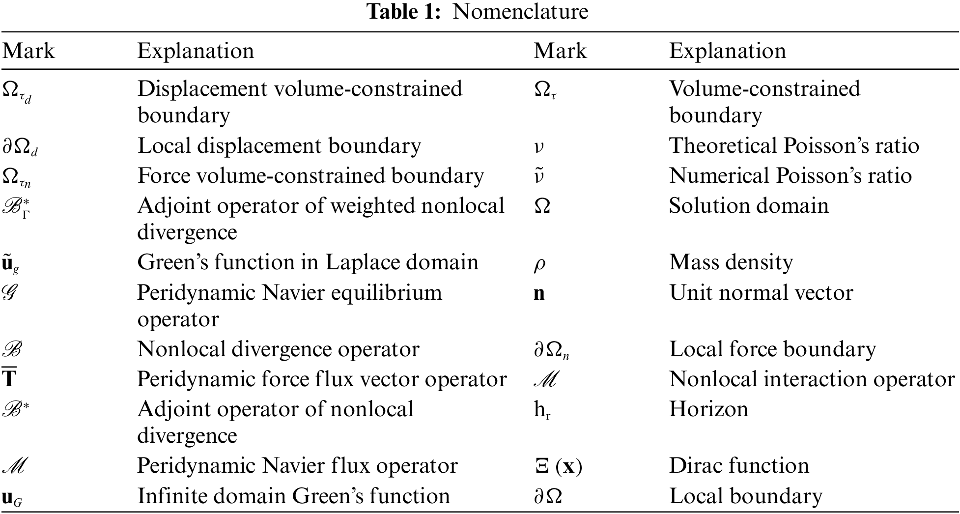
The process of outlining the BEM for OSPD, referred to as OSPD-BEM, unfolds through the following steps. Firstly, a boundary integral equation (BIE) for OSPD is derived, drawing support from Green’s function [34,35] and the nonlocal operator theory [36,37] in Section 2. Following this, a crack propagation model for the OSPD-BEM is proposed in Section 3. In Section 4, the accuracy and efficiency of OSPD-BEM are then demonstrated through the presentation of four numerical examples. The conclusions are given in Section 5. For ease of reading, the symbols in the paper are listed in Table 1 before the text begins.
2 The Boundary Integral Equation
Firstly, we briefly introduce the linear elastic OSPD [38,39] with the volume-constrained boundary [40,41]. The equilibrium equation for the linear elastic OSPD is as follows [37]:
where
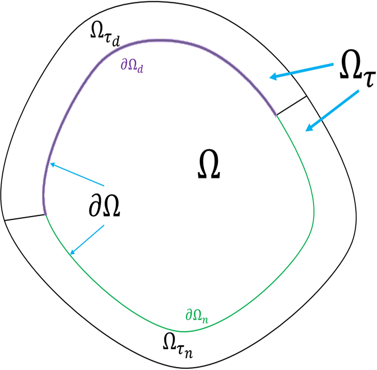
Figure 1: The diagram for volume-constrained boundary (color online)
in which
For the two-dimensional problem, material parameters
It is noteworthy that the literature [5,43] also give the similar nonlocal operators. The connection of both nonlocal operators is in Appendix A.
Stemming from simplifying form, we introduce the following notations:
For two instances with different body forces and boundary constraints, Eq. (1) can be rewritten as
Following the derivations of the reciprocal theorem of the BBPD in [21], we can obtain the reciprocal theorem for OSPD
whose form is consistent with that of bond-based PD except for the operators defined in Eqs. (13) and (14). The integrals on the left side and right one respectively denote internal integrals and volume-constrained boundary integrals. One can find that the boundary integrals are also volume integrals, which deprives the advantage of the dimensionality reduction for the BEM. Thus we introduce an extra condition to the volume-constrained boundary, which converts the integral on the right side of Eq. (15) from the one in the volume-constrained boundary to the one on the local boundary. The equivalency relationship to transform the integral in volume-constrained boundary
where
Substituting Eqs. (20) and (21) into Eq. (15), the reciprocal theorem is rewritten as
which builds up a connection between internal integrals and classical boundary integrals, and is a precondition of BIE that will be derived as follows.
Imitating opinion in traditional BEM [46]. We take into account
Applying first equations for Eqs. (23) and (24) to (26), we obtain
Executing limit analysis
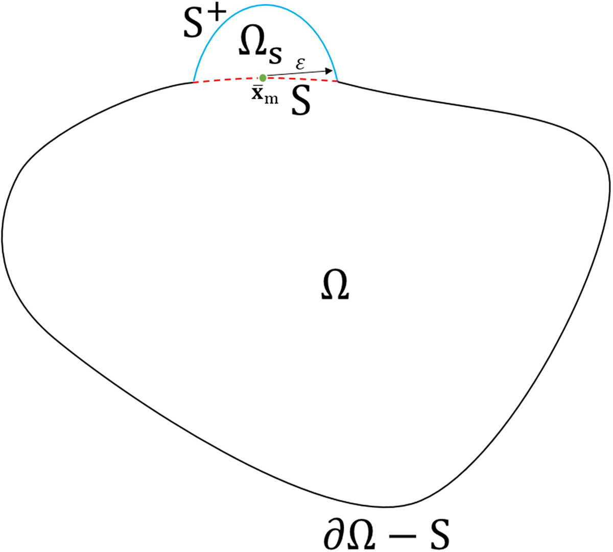
Figure 2: The diagram for the boundary limit process [21] (color online)
The result for the integral on left side of Eq. (28) is
where
Adopting an approach in the literature [47,48] to build up a relation between PD boundary constraints and local boundary constraints, we obtain the following relationship:
where
which is the BIE of OSPD for the static case. For the dynamic case, we give BIE corresponding to the Laplace domain in Appendix B. Once a displacement and force flux on the local boundary
The crack propagation model for the OSPD-BEM proposed in this paper is inspired by the cohesive crack model [29–31] and the PD bilinear model [32,33]. We take a continuum medium in Fig. 3 as an example, and the construction of the model is given as follows.

Figure 3: The diagram of the crack propagation model (color online)
In Fig. 3,

Figure 4: The diagram for the crack propagation model in the elastic stage (color online)
where
For the crack propagation model, we consider that the fracture at any material point

Figure 5: The diagram for the fracture calculation model in the defunct stage (color online)
Figure 6: The diagram of the crack propagation model in the adhesive stage (color online)
The force flux vector
We assume that the force flux vector

Figure 7: The diagram for the constitutive relationship in the adhesive stage (color online)
where
where
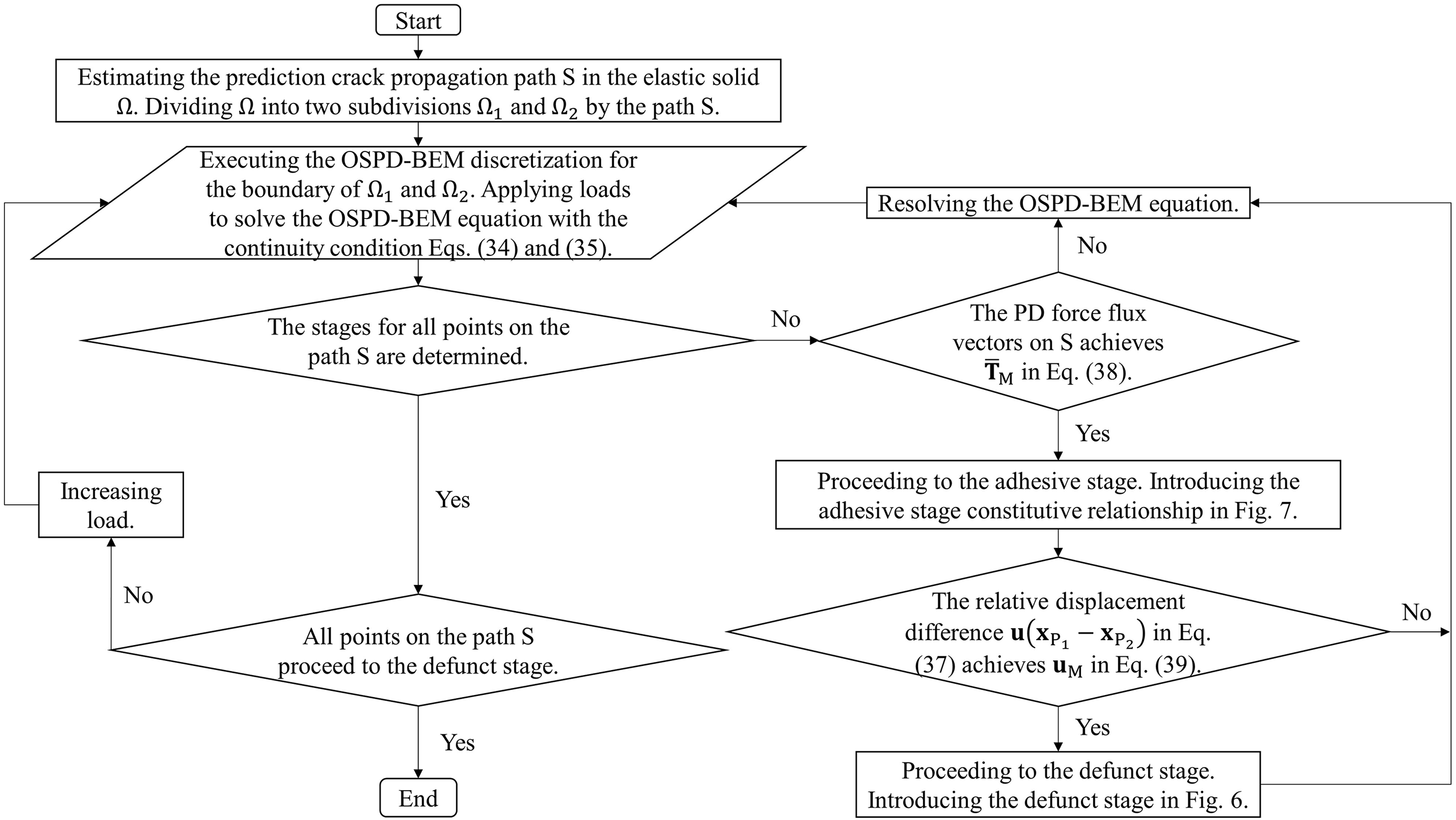
Figure 8: The flow chart for the solving process of the crack propagation model
We will take four numerical examples to confirm the accuracy and efficiency of OSPD-BEM in this section. Firstly, a two-dimensional square plate under uniaxial loading is investigated to estimate the numerical Poisson’s ratio as those in the literature [53,54]. It displays that our numerical method can be more accurate than the PD-MPM. Secondly, we discuss the crack initiation in a double-notched specimen as the literature [21], which reveals the accuracy and efficiency of the OSPD-BEM compared with the PD-MPM. Thirdly, the wedge-splitting test is simulated to research a fracture toughness for the concrete specimen [55,56], and its result is compared to experimental results, which displays again the the accuracy and efficiency of OSPD-BEM. Finally, a three-point bending experiment is executed.
4.1 Two-Dimensional Square Plate under Uniaxial Loading
We consider a two-dimensional square plate withstanding the uniaxial tensile loading in the direction
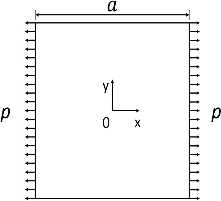
Figure 9: The diagram for stretching square plate
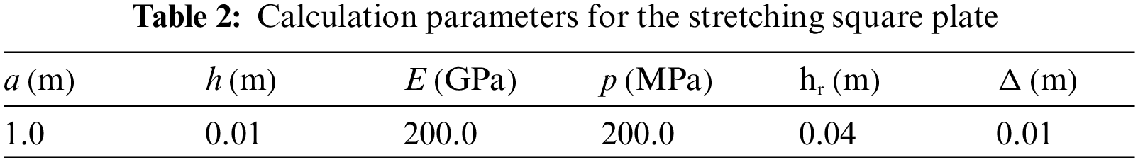
where
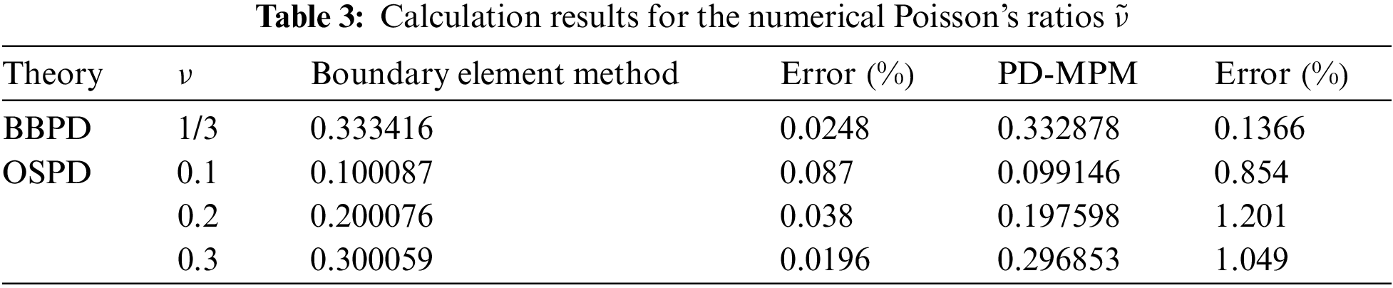
From Table 3, one can find that the errors of the OSPD-BEM are much smaller than those of PD-MPM. Besides, the numerical Poisson’s ratios predicted by the PD-MPM are always lower than the given Poisson’s ratio, which can be due to a spurious boundary softening phenomena [57]. This phenomenon is observed from the results of PD-MPM in Fig. 10. We find that Poisson’s ratio is variable for the OSPD in Table 3, while it is the fixed value for the BBPD. The BBPD-BEM is one order of magnitude more precise than the PD-MPM, while the magnitude is two orders for the OSPD-BEM. The reason is that the spurious boundary softening phenomena [57] is more serious for the OSPD compared with the BBPD.

Figure 10: Displacement predicted by the PD-MPM and the OSPD-BEM for
4.2 Two-Dimensional Crack Initiation in a Double-Notched Specimen
In this example, we consider a crack initiation problem in the square plate with a double-notched edge crack exerted uniaxial tensile loading displayed in Fig. 11. The calculation parameters are exhibited in Table 4. E denotes elastic modulus;

Figure 11: The diagram for a double-notched specimen (color online)
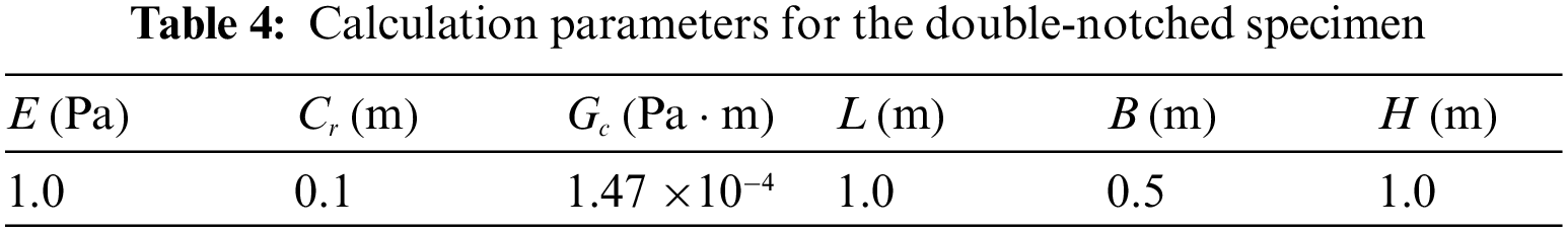
For Poisson’s ratio
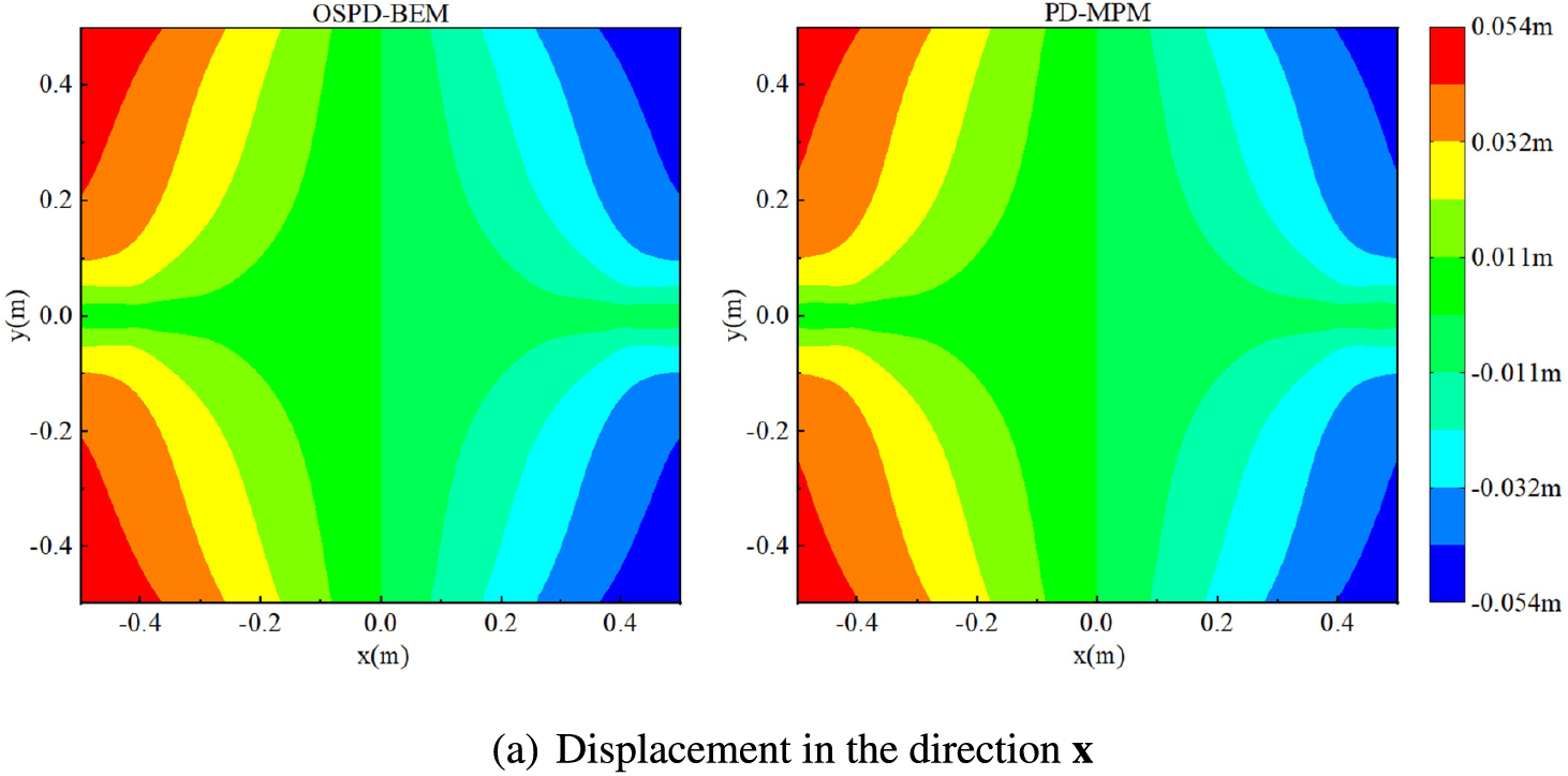
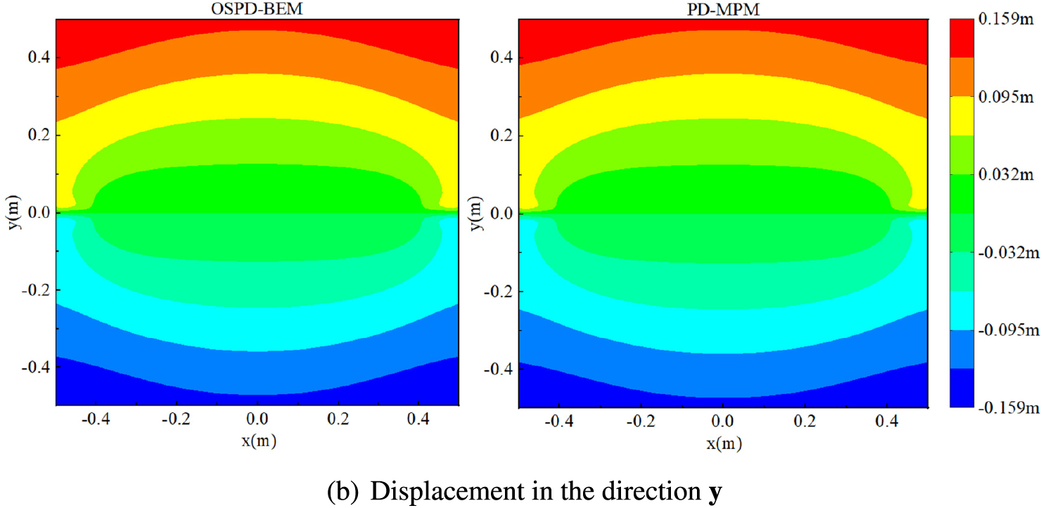
Figure 12: Displacement predicted by the OSPD-BEM and PD-MPM for
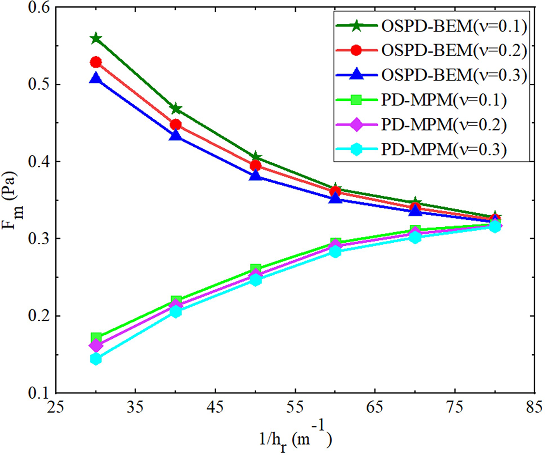
Figure 13: The load
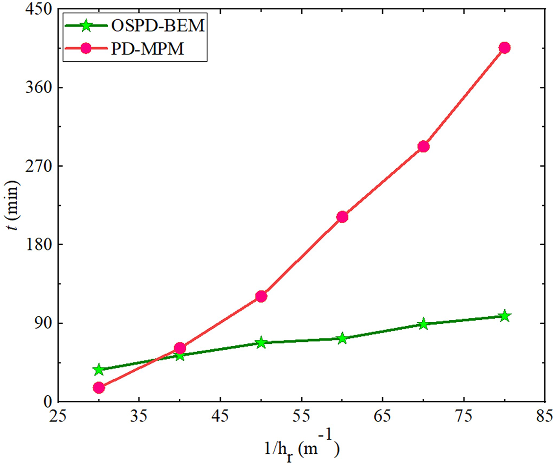
Figure 14: The calculation time
In Fig. 13, we find the utmost load
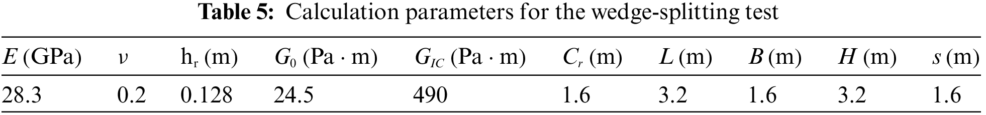
The wedge-splitting test is a significant experiment to investigate the fracture toughness of the concrete specimen [55,56]. Many numerical methods based on classical continuum mechanics [59,60] and PD theory [32,61] have been applied to simulate this experiment. In this section, the OSPD-BEM is used to simulate this experiment process, and our result will be compared with those of the ordinary state-based peridynamic mesh-free particle method (OSPD-MPM) predicted by Bie et al. [61]. The schematics of the wedge-splitting test specimen is displayed in Fig. 15. The relative displacement
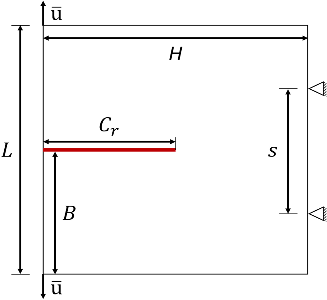
Figure 15: The schematics for the wedge-splitting test specimen (color online)
To describe the propagation process of a crack, the curve of the crack length vs. the crack mouth opening displacement (CMOD) is given in Fig. 16. Some specific crack propagation diagrams are shown in Fig. 17. The main purpose of the wedge-splitting test is to obtain the curve about the external load vs. CMOD. This curve is related to the fracture toughness of a concrete specimen [55]. Drawing upon the crack propagation model of the OSPD-BEM in Section 3, the curve of the load vs. the CMOD is given in Fig. 18. In Fig. 18, we find the result of the OSPD-BEM is closer to the experimental result [56] than the one of PD-MPM in [61]. The reasons originate from two aspects. First, the OSPD-BEM is more accurate as a semi-analytical calculation method. Second, the softening process observed in the test [60,62] is introduced into the crack propagation model.
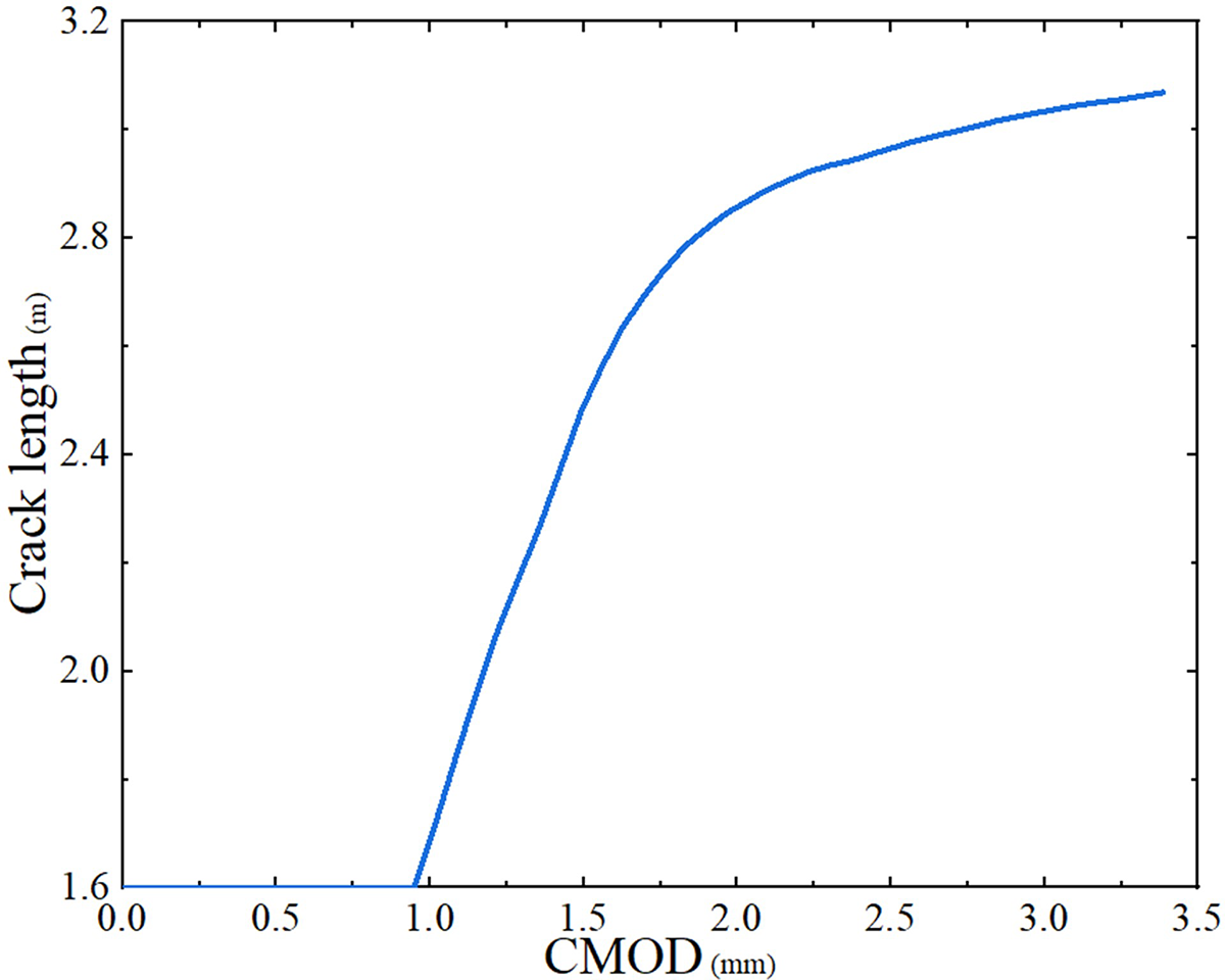
Figure 16: The crack length vs. the CMOD (color online)
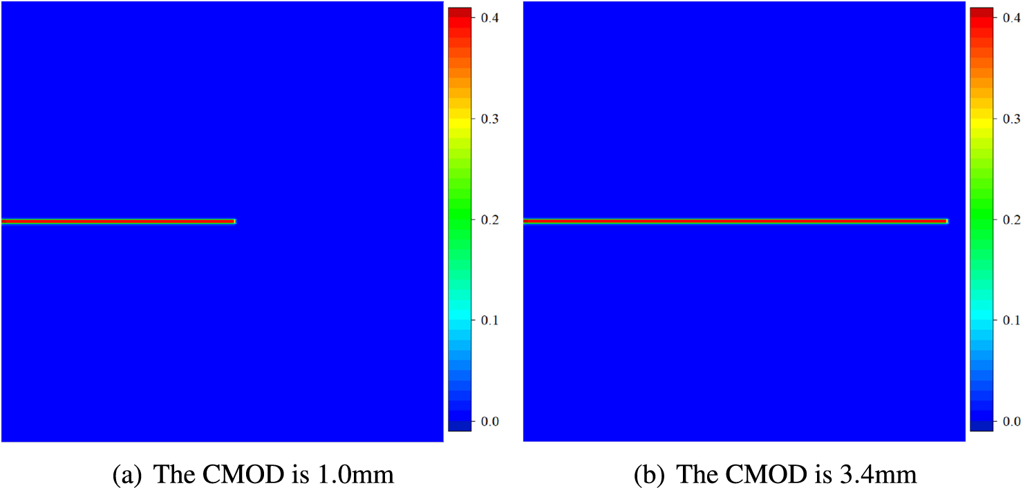
Figure 17: The crack propagation diagram (color online)
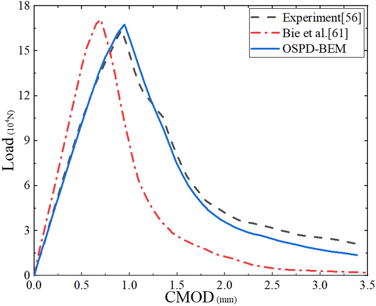
Figure 18: The load vs. the CMOD (color online)
The crack initiation load

Considering the calculation efficiency, we find that it takes 44000 s to simulate the wedge-splitting test in Fig. 15 with the OSPD-MPM [61], while the time consumption has been reduced to 21000 s with the coupling method [61] between the OSPD-MPM and the node-based smoothed finite element method (NS-FEM). Nevertheless, the OSPD-BEM only takes 11000 s to deal with the same problem in Fig. 15. The calculation efficiency is respectively improved by three times and one time compared with the OSPD-MPM [61] and the coupling method [61]. By the way, 200 boundary elements are used in the OSPD-BEM for the simulation result in Fig. 15. The computer equipment is displayed as (1) CPU: 12th Gen Intel(R) Core(TM) i5-1240P 1.70 GHz; (2) RAM: 16.0 GB; (3) OS: Windows 11 Home 22H2 64 bit.
The three-point bending experiment is the main experimental approach to measure the mechanical properties of materials [63,64]. The beam with a central crack is executed by the three-point bending experimental to investigate fracture toughness in Fig. 19. As displayed in Fig. 19,
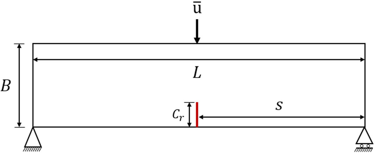
Figure 19: The schematics for the three-point bending test specimen (color online)
The geometry and materials parameters are shown in Table 7. In Table 7, E denotes elastic modulus;
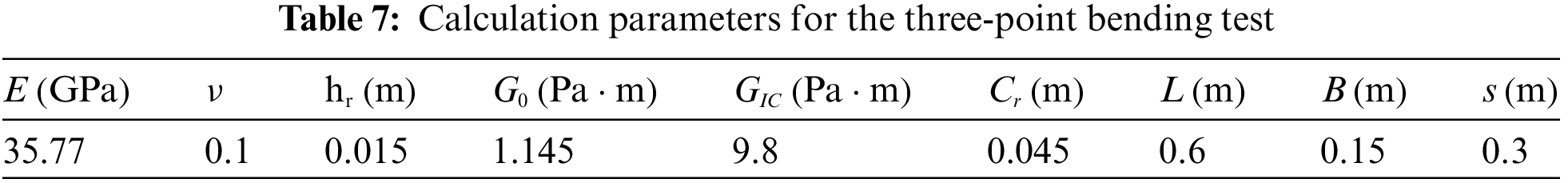
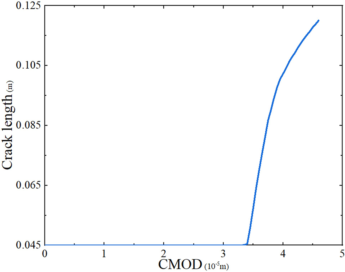
Figure 20: The crack length vs. the CMOD (color online)

Figure 21: The crack propagation diagram (color online)
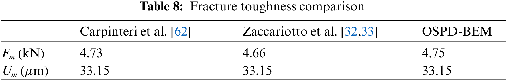
The curved line of external load vs. CMOD is given in Fig. 22, and we compare OSPD-BEM results with FEM results predicted by Carpinteri et al. [62] and the bond-based peridynamic mesh-free particle method (BBPD-MPM) results predicted by Zaccariotto et al. [32,33] in Fig. 22. We find the result of the OSPD-BEM is closer to those of Carpinteri et al. [62] than those of Zaccariotto et al. [32,33]. The reason stems from the effect of Poisson’s ratio. The OSPD-BEM and Carpinteri et al. [62] can adopt a real Poisson’s ratio, while Zaccariotto et al. [32,33] is trapped in a fixed Poisson’s ratio. As displayed in [65], the effect of Poisson’s ratio becomes obvious, when a crack approaches boundary. The crack initiation load
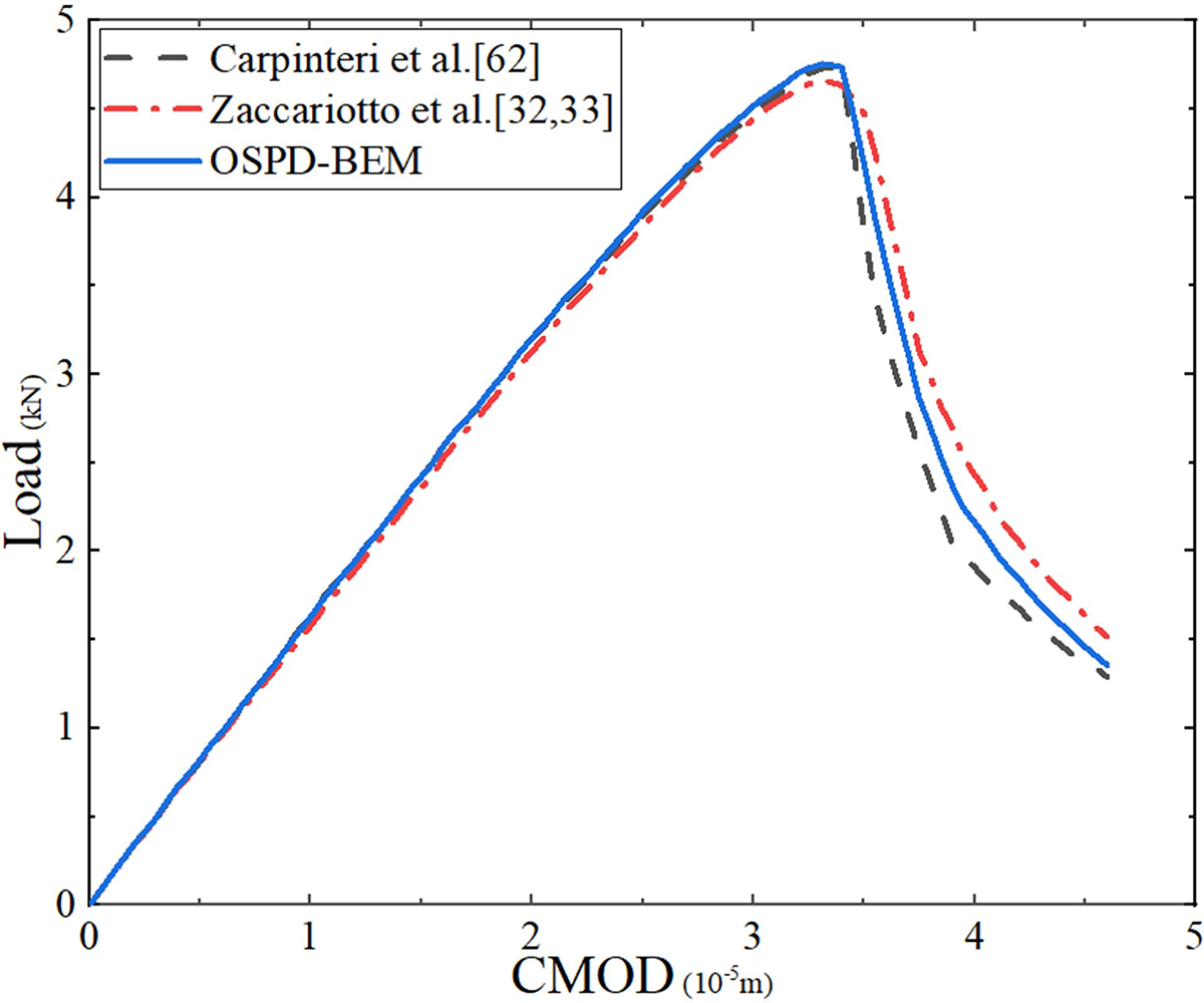
Figure 22: The load vs. the CMOD (color online)
In our research, we propose OSPD-BEM as an enhancement over prior efforts [21]. This method inherits the advantages of the BBPD-BEM [21]. Firstly, it eliminates the boundary softening phenomenon [57] resulting from boundary discretization. Secondly, it facilitates problem-solving in infinite domains. Thirdly, it exhibits advantages in terms of accuracy and efficiency compared to numerical methods that discretize the entire domain. In addition, this method is based on the OSPD, overcoming theoretical limitations present in previous works [21], such as fixed Poisson’s ratio. Furthermore, we introduce a fracture calculation model tailored for OSPD-BEM to investigate basic crack propagation problems. In future research, a viable approach to tackling complex crack growth problems, such as multiple cracks and crack branching, might involve the utilization of a coupling method [66,67]. This method would integrate PD-MPM and OSPD-BEM in a complementary manner, with PD-MPM applied in cracked regions and OSPD-BEM in uncracked regions.
Acknowledgement: We acknowledge the High-Performance Computing Platform of Peking University for providing computational resources.
Funding Statement: The work is supported by the National Key R&D Program of China (2020YFA0710500).
Author Contributions: The authors confirm contribution to the paper as follows: study conception and design: Xue Liang, Linjuan Wang; data collection: Xue Liang; analysis and interpretation of results: Xue Liang, Linjuan Wang; draft manuscript preparation: Xue Liang, Linjuan Wang. All authors reviewed the results and approved the final version of the manuscript.
Availability of Data and Materials: The data that support the findings of this study are available from the corresponding author upon reasonable request.
Conflicts of Interest: The authors declare that they have no conflicts of interest to report regarding the present study.
References
1. Silling, S. A. (2000). Reformulation of elasticity theory for discontinuities and long-range forces. Journal of the Mechanics and Physics of Solids, 48(1), 175–209. https://doi.org/10.1016/S0022-5096(99)00029-0 [Google Scholar] [CrossRef]
2. Silling, S. A., Epton, M., Weckner, O., Xu, J., Askari, E. (2007). Peridynamic states and constitutive modeling. Journal of Elasticity, 88, 151–184. https://doi.org/10.1007/s10659-007-9125-1 [Google Scholar] [CrossRef]
3. Ren, H., Zhuang, X., Rabczuk, T. (2017). Dual-horizon peridynamics: A stable solution to varying horizons. Computer Methods in Applied Mechanics and Engineering, 318, 762–782. https://doi.org/10.1016/j.cma.2016.12.031 [Google Scholar] [CrossRef]
4. Ren, H., Zhuang, X., Cai, Y., Rabczuk, T. (2016). Dual-horizon peridynamics. International Journal for Numerical Methods in Engineering, 108(12), 1451–1476. https://doi.org/10.1002/nme.5257 [Google Scholar] [CrossRef]
5. Rabczuk, T., Ren, H., Zhuang, X. (2019). A nonlocal operator method for partial differential equations with application to electromagnetic waveguide problem. Computers, Materials & Continua, 59(1), 31–55. https://doi.org/10.32604/cmc.2019.04567 [Google Scholar] [CrossRef]
6. Liu, S., Fang, G., Liang, J., Fu, M., Wang, B. (2020). A new type of peridynamics: Element-based peridynamics. Computer Methods in Applied Mechanics and Engineering, 366, https://doi.org/10.1016/j.cma.2020.113098 [Google Scholar] [CrossRef]
7. Liu, S., Fang, G., Liang, J., Fu, M., Wang, B. et al. (2021). Study of three-dimensional Euler-Bernoulli beam structures using element-based peridynamic model. European Journal of Mechanics/A Solids, 86, 104186. https://doi.org/10.1016/j.euromechsol.2020.104186 [Google Scholar] [CrossRef]
8. Tian, D., Zhou, X. (2022). A viscoelastic model of geometry-constraint-based non-ordinary state-based peridynamics with progressive damage. Computational Mechanics, 69, 1413–1441. https://doi.org/10.1007/s00466-022-02148-z [Google Scholar] [CrossRef]
9. Xiao, Y., Wu, J., Shen, H., Hu, X., Yong, H. (2023). Damage behavior in Bi-2212 round wire with 3D elastoplastic peridynamic. Acta Mechanica Sinica, 39, https://doi.org/10.1007/s10409-023-22431-x [Google Scholar] [CrossRef]
10. Liu, D., Liu, N., Zhou, W. (2017). Peridynamic modelling of impact damage in three-point bending beam with offset notch. Applied Mathematics and Mechanics (English Edition), 38(1), 99–110. https://doi.org/10.1007/s10483-017-2158-6 [Google Scholar] [CrossRef]
11. Wang, X., Tong, Q. (2023). Peridynamic modeling of delayed fracture in electrodes during lithiation. Computer Methods in Applied Mechanics and Engineering, 404, 115774. https://doi.org/10.1016/j.cma.2022.115774 [Google Scholar] [CrossRef]
12. Ongaro, G., Bertani, R., Galvanetto, U., Pontefisso, A., Zaccariotto, M. (2022). A multiscale peridynamic framework for modelling mechanical properties of polymer-based nanocomposites. Engineering Fracture Mechanics, 274, 108751. https://doi.org/10.1016/j.engfracmech.2022.108751 [Google Scholar] [CrossRef]
13. Wu, P., Chen, Z. (2023). Peridynamic electromechanical modeling of damaging and cracking in conductive composites: A stochastically homogenized approach. Composite Structures, 305, 116528. https://doi.org/10.1016/j.compstruct.2022.116528 [Google Scholar] [CrossRef]
14. Silling, S. A., Fermen-Coker, M. (2021). Peridynamic model for microballistic perforation of multilayer graphene. Theoretical and Applied Fracture Mechanics, 113, 102947. https://doi.org/10.1016/j.tafmec.2021.102947 [Google Scholar] [CrossRef]
15. Nowak, M., Mulewska, K., Azarov, A., Kurpaska, L., Ustrzycka, A. (2023). A peridynamic elasto-plastic damage model for ion-irradiated materials. International Journal of Mechanical Sciences, 237, 107806. https://doi.org/10.1016/j.ijmecsci.2022.107806 [Google Scholar] [CrossRef]
16. Yang, S., Gu, X., Zhang, Q., Xia, X. (2021). Bond-associated non-ordinary state-based peridynamic model for multiple spalling simulation of concrete. Acta Mechanica Sinica, 37(7), 1104–1135. https://doi.org/10.1007/s10409-021-01055-5 [Google Scholar] [CrossRef]
17. Silling, S. A., Askari, E. (2005). A meshfree method based on the peridynamic model of solid mechanics. Theoretical and Applied Fracture Mechanics, 83(17–18), 1526–1535. https://doi.org/10.1016/j.compstruc.2004.11.026 [Google Scholar] [CrossRef]
18. Kilic, B., Madenci, E. (2009). Structural stability and failure analysis using peridynamic theory. International Journal of Non-Linear Mechanics, 44(8), 845–854. https://doi.org/10.1016/j.ijnonlinmec.2009.05.007 [Google Scholar] [CrossRef]
19. Chen, X., Gunzburger, M. (2011). Continuous and discontinuous finite element methods for a peridynamics model of mechanics. Computer Methods in Applied Mechanics and Engineering, 200(9–12), 1237–1250. https://doi.org/10.1016/j.cma.2010.10.014 [Google Scholar] [CrossRef]
20. Tian, X., Du, Q. (2013). Analysis and comparison of different approximation to nonlocal diffusion and linear peridynamic equations. Siam Journal on Numerical Analysis, 51(6), 3458–3482. https://doi.org/10.1137/13091631X [Google Scholar] [CrossRef]
21. Liang, X., Wang, L., Xu, J., Wang, J. (2021). The boundary element method of peridynamics. International Journal for Numerical Methods in Engineering, 122(20), 5558–5593. https://doi.org/10.1002/nme.6764 [Google Scholar] [CrossRef]
22. Liu, W., Hong, J. W. (2012). A coupling approach of discretized peridynamics with finite element method. Computer Methods in Applied Mechanics and Engineering, 245–246, 163–175. https://doi.org/10.1016/j.cma.2012.07.006 [Google Scholar] [CrossRef]
23. Fang, G., Liu, S., Fu, M., Wang, B., Wu, Z. et al. (2019). A method to couple state-based peridynamics and finite element method for crack propagation problem. Mechanics Research Communications, 95, 89–95. https://doi.org/10.1016/j.mechrescom.2019.01.005 [Google Scholar] [CrossRef]
24. Dong, Y., Su, C., Qiao, P. (2020). A stability-enhanced peridynamic element to couple non-ordinary state-based peridynamics with finite element method for fracture analysis. Finite Elements in Analysis and Design, 181, 103480. https://doi.org/10.1016/j.finel.2020.103480 [Google Scholar] [CrossRef]
25. Yang, Y., Liu, Y. (2021). Modeling of cracks in two-dimensional elastic bodies by coupling the boundary element method with peridynamics. International Journal of Solids and Structures, 217–218, 74–89. https://doi.org/10.1016/j.ijsolstr.2021.02.002 [Google Scholar] [CrossRef]
26. Yang, Y., Liu, Y. (2022). Analysis of dynamic crack propagation in two-dimensional elastic bodies by coupling the boundary element method and the bond-based peridynamics. Computer Methods in Applied Mechanics and Engineering, 399, 115339. https://doi.org/10.1016/j.cma.2022.115339 [Google Scholar] [CrossRef]
27. Kan, X., Zhang, A., Yan, J., Wu, W., Liu, Y. (2020). Numerical investigation of ice breaking by a high-pressure bubble based on a coupled BEM-PD model. Journal of Fluids and Structures, 96, 103016. https://doi.org/10.1016/j.jfluidstructs.2020.103016 [Google Scholar] [CrossRef]
28. Chen, X., Yu, H. (2022). A multiscale method coupling peridynamic and boundary element models for dynamic problems. Computer Methods in Applied Mechanics and Engineering, 401, 115669. https://doi.org/10.1016/j.cma.2022.115669 [Google Scholar] [CrossRef]
29. Barenblatt, G. I. (1959). The formation of equilibrium cracks during brittle fracture: General ideas and hypothesis, axially symmetric cracks. Journal of Applied Mathematics and Mechanics, 23(3), 622–636. https://doi.org/10.1016/0021-8928(59)90157-1 [Google Scholar] [CrossRef]
30. Dugdale, D. S. (1960). Yielding of steel sheets containing slits. Journal of the Mechanics and Physics of Solids, 8(2), 100–104. https://doi.org/10.1016/0022-5096(60)90013-2 [Google Scholar] [CrossRef]
31. Hillerborg, A., Modeer, M., Petersson, P. E. (1976). Analysis of crack formation and crack growth in concrete by means of fracture mechanics and finite elements. Cement and Concrete Research, 6(6), 773–781. https://doi.org/10.1016/0008-8846(76)90007-7 [Google Scholar] [CrossRef]
32. Zaccariotto, M., Luongo, F., Sarego, G., Galvanetto, U. (2015). Examples of applications of the peridynamic theory to the solution of static equilibrium problems. The Aeronautical Journal, 119(1216), 677–700. https://doi.org/10.1017/S0001924000010770 [Google Scholar] [CrossRef]
33. Zaccariotto, M., Mudric, T., Tomasi, D., Shojaei, A., Galvanetto, U. (2018). Coupling of FEM meshes with peridynamic grids. Computer Methods in Applied Mechanics and Engineering, 330, 471–497. https://doi.org/10.1016/j.cma.2017.11.011 [Google Scholar] [CrossRef]
34. Wang, L., Xu, J., Wang, J. (2019). Elastodynamics of linearized isotropic state-based peridynamic media. Journal of Elasticity, 137(2), 157–176. https://doi.org/10.1007/s10659-018-09723-7 [Google Scholar] [CrossRef]
35. Wang, L. (2018). Research on some basic problems of spatiotemporal non-local elasticity (Ph.D. Thesis). Peking University, China. [Google Scholar]
36. Du, Q., Burgunder, M., Lehoucq, R. B., Zhou, K. (2013). A nonlocal vector calculus, nonlocal volume-constrained problems, and nonlocal balance laws. Mathematical Models and Methods in Applied Sciences, 23(3), 493–540. https://doi.org/10.1142/S0218202512500546 [Google Scholar] [CrossRef]
37. Du, Q., Gunzburger, M., Lehoucq, R. B., Zhou, K. (2013). Analysis of the volume-constrained peridynamic Navier equation of linear elasticity. Journal of Elasticity, 113(2), 193–217. https://doi.org/10.1007/s10659-012-9418-x [Google Scholar] [CrossRef]
38. Silling, S. A. (2010). Linearized theory of peridynamic states. Journal of Elasticity, 99, 85–111. https://doi.org/10.1007/s10659-009-9234-0 [Google Scholar] [CrossRef]
39. Sarego, G., Le, Q. V., Bobaru, F., Zaccariotto, M., Galvanetto, U. (2016). Linearized state-based peridynamics for 2D problems. International Journal for Numerical Methods in Engineering, 108(10), 1174–1197. https://doi.org/10.1002/nme.5250 [Google Scholar] [CrossRef]
40. Du, Q., Gunzburger, M., Lehoucq, R. B., Zhou, K. (2012). Analysis and approximation of nonlocal diffusion problems with volume constraints. SIAM Review, 54(4), 667–696. https://doi.org/10.1137/110833294 [Google Scholar] [CrossRef]
41. Mengesha, T., Du, Q. (2014). Nonlocal constrained value problems for a linear peridynamic Navier equation. Journal of Elasticity, 116, 27–51. https://doi.org/10.1007/s10659-013-9456-z [Google Scholar] [CrossRef]
42. Seleson, P., Parks, M. L. (2011). On the role of the influence function in the peridynamic theory. Journal for Multiscale Computational Engineering, 9(6), 689–706. https://doi.org/10.1615/IntJMultCompEng.2011002527 [Google Scholar] [CrossRef]
43. Ren, H., Zhuang, X., Rabczuk, T. (2020). A nonlocal operator method for solving partial differential equations. Computer Methods in Applied Mechanics and Engineering, 358, 112621. https://doi.org/10.1016/j.cma.2019.112621 [Google Scholar] [CrossRef]
44. Lehoucq, R. B., Silling, S. A. (2008). Force flux and the peridynamic stress tensor. Journal of the Mechanics and Physics of Solids, 56(4), 1566–1577. https://doi.org/10.1016/j.jmps.2007.08.004 [Google Scholar] [CrossRef]
45. Silling, S. A., Lehoucq, R. B. (2008). Convergence of peridynamics to classical elasticity theory. Journal of Elasticity, 93, 13–37. https://doi.org/10.1007/s10659-008-9163-3 [Google Scholar] [CrossRef]
46. Aliabadi, M. H. (2002). The boundary element method. London: John Wiley and Sons. [Google Scholar]
47. Scabbia, F., Zaccariotto, M., Galvanetto, U. (2021). A novel and effective way to impose boundary conditions and to mitigate the surface effect in state-based peridynamics. International Journal for Numerical Methods in Engineering, 122(20), 5773–5811. https://doi.org/10.1002/nme.6773 [Google Scholar] [CrossRef]
48. Scabbia, F., Zaccariotto, M., Galvanetto, U. (2022). A new method based on Taylor expansion and nearest-node strategy to impose Dirichlet and Neumann boundary conditions in ordinary state-based peridynamics. Computational Mechanics, 70, 1–27. https://doi.org/10.1007/s00466-022-02153-2 [Google Scholar] [CrossRef]
49. Tong, Y., Shen, W., Shao, J., Chen, J. (2020). A new bond model in peridynamics theory for progressive failure in cohesive brittle materials. Engineering Fracture Mechanics, 223, 106767. https://doi.org/10.1016/j.engfracmech.2019.106767 [Google Scholar] [CrossRef]
50. Tong, Y., Shen, W., Shao, J. (2020). An adaptive coupling method of state-based peridynamics theory and finite element method for modeling progressive failure process in cohesive materials. Computer Methods in Applied Mechanics and Engineering, 370, 113248. https://doi.org/10.1016/j.cma.2020.113248 [Google Scholar] [CrossRef]
51. Madenci, E., Oterkus, E. (2014). Peridynamic theory and its applications. New York: Springer. [Google Scholar]
52. Zehnder, A. T. (2012). Fracture mechanics. London: Springer. [Google Scholar]
53. Prakash, N., Seidel, G. D. (2015). A novel two-parameter linear elastic constitutive model for bond based peridynamics. 56th AIAA/ASCE/AHS/ASC Structures, Structural Dynamics, and Materials Conference, Kissimmee, USA. [Google Scholar]
54. Huang, X., Li, S., Jin, Y., Yang, D., Su, G. et al. (2019). Analysis on the influence of Poisson’s ratio on brittle fracture by applying uni-bond dual-parameter peridynamic model. Engineering Fracture Mechanics, 222, 106685. https://doi.org/10.1016/j.engfracmech.2019.106685 [Google Scholar] [CrossRef]
55. Bruhwiler, E., Wittmann, F. H. (1990). The wedge splitting test, a new method of performing stable fracture mechanics tests. Engineering Fracture Mechanics, 35(1–3), 117–125. https://doi.org/10.1016/0013-7944(90)90189-N [Google Scholar] [CrossRef]
56. Trunk, B. (2000). Einfluss der Bauteilgroesse auf die Bruchenergie von Beton. German: Aedificatio Publishers. [Google Scholar]
57. Le, Q. V., Bobaru, F. (2018). Surface corrections for peridynamic models in elasticity and fracture. Computational Mechanics, 61, 499–518. https://doi.org/10.1007/s00466-017-1469-1 [Google Scholar] [CrossRef]
58. Tian, X., Du, Q., Gunzburger, M. (2016). Asymptotically compatible schemes for the approximation of fractional Laplacian and related nonlocal diffusion problems on bounded domains. Advances in Computational Mathematics, 42(6), 1363–1380. https://doi.org/10.1007/s10444-016-9466-z [Google Scholar] [CrossRef]
59. Areias, P. M. A., Belytschko, T. (2005). Analysis of three-dimensional crack initiation and propagation using the extended finite element method. International Journal for Numerical Methods in Engineering, 63(5), 760–788. https://doi.org/10.1002/nme.1305 [Google Scholar] [CrossRef]
60. Su, X., Yang, Z., Liu, G. (2010). Finite element modelling of complex 3D static and dynamic crack propagation by embedding cohesive elements in abaqus. Acta Mechanica Solida Sinica, 23(3), 271–282. https://doi.org/10.1016/S0894-9166(10)60030-4 [Google Scholar] [CrossRef]
61. Bie, Y., Cui, X., Li, Z. (2018). A coupling approach of state-based peridynamics with node-based smoothed finite element method. Computer Methods in Applied Mechanics and Engineering, 331, 675–700. https://doi.org/10.1016/j.cma.2017.11.022 [Google Scholar] [CrossRef]
62. Carpinteri, A., Colombo, G. (1989). Numerical analysis of catastrophic softening behaviour (snap-back instability). Computers and Structures, 31(4), 607–636. https://doi.org/10.1016/0045-7949(89)90337-4 [Google Scholar] [CrossRef]
63. Dufort, L., Grediac, M., Surrel, Y. (2001). Experimental evidence of the cross-section warping in short composite beams under three point bending. Composite Structures, 51(1), 37–47. https://doi.org/10.1016/S0263-8223(00)00121-5 [Google Scholar] [CrossRef]
64. Zhang, J., Dong, W., Zhang, B. (2023). Experimental study on local crack propagation of concrete under three-point bending. Construction and Building Materials, 401, 132699. https://doi.org/10.1016/j.conbuildmat.2023.132699 [Google Scholar] [CrossRef]
65. Sundaram, V. K. A., Madenci, E. (2023). Direct coupling of dual-horizon peridynamics with finite elements for irregular discretization without an overlap zone. Engineering with Computers, 40, 605–635. https://doi.org/10.1007/s00366-023-01800-3 [Google Scholar] [CrossRef]
66. Han, F., Lubineau, G. (2012). Coupling of nonlocal and local continuum models by the Arlequin approach. Journal for Numerical Methods in Engineering, 89(6), 671–685. https://doi.org/10.1002/nme.3255 [Google Scholar] [CrossRef]
67. Han, F., Lubineau, G., Azdoud, Y., Askari, A. (2016). A morphing approach to couple state-based peridynamics with classical continuum mechanics. Computer Methods in Applied Mechanics and Engineering, 301, 336–358. https://doi.org/10.1016/j.cma.2015.12.024 [Google Scholar] [CrossRef]
Appendix A. The Comparison of Different Nonlocal Operators
The literature [36] and the literature [5,43] provide two different nonlocal operators, and both can effectively represent the PD equilibrium equation and boundary condition. The nonlocal gradient, nonlocal curl and nonlocal divergence in both literature is a dual relationship. The nonlocal operators [5,43] is the weighted adjoint operator of the ones [36], if the following conditions are satisfied:
where the symbol on the left side of Eq. (A.1) appears in Eqs. (6) and (7), and the symbol on the right side of Eq. (A.1) appears in Eq. (6) of the literature [43].
In other words, there are
where
The following conditions are satisfied:
Then
where the symbols are seen in Eq. (13) of the literature [43].
Appendix B. The Boundary Integral Equation in the Laplace Domain
It is convenient to deal with the dynamic problem in the Laplace domain for the BEM. It has two prominent advantages, compared with time domain. The first is eliminating time accumulation error; the second is that we can easily implement parallel computation. Thus, we derive the BIE of the OSPD for dynamic problems in Laplace domain as follows. First of all, we give the dynamic equation for the linear elastic OSPD in the Laplace domain
where the operators
The weighted residual method is adopted to derive the BIE in Laplace domain instead of the reciprocal theorem, following the derivation in the classical theory. We rewrite Eq. (B.1) in the form of weighted residual as follows:
where
where
We find that if
Substituting Eq. (B.6) into Eq. (B.2), we obtain
Substituting Eqs. (B.1) and (B.3) into Eq. (B.7) and dividing the integral domain
Considering the extra condition Eq. (16), which converts the integral in the volume constrained boundary to the one on the classical boundary, we simplify Eq. (B.8) as follows:
where
Eq. (B.13) is the BIE of the OSPD in the Laplace domain.
Cite This Article
 Copyright © 2024 The Author(s). Published by Tech Science Press.
This work is licensed under a Creative Commons Attribution 4.0 International License , which permits unrestricted use, distribution, and reproduction in any medium, provided the original work is properly cited.
 Downloads
 Citation Tools