Buckling Optimization of Curved Grid Stiffeners through the Level Set Based Density Method

1  Introduction

Stiffened structures are commonly used in various fields because of their efficient material utilization and superior mechanical properties [1,2], for instance, in aircraft fuselages, wing skins, and others. Correspondingly, the study of its stability has important engineering implications. It is well known that buckling failure is a common failure mode of stiffened structures under axial compression [3], and it is important for their design and applications.

The Optimal design of stiffened structures taking into account the buckling properties has attracted the attention of many researchers and much effort has been devoted to it. Kapania et al. [4,5] indicated that some curved stiffeners placed on the metal plates and composite plates with buckling-dominated load may further reduce the weight of the structure with respect to the straight stiffeners under the same load. Tamijani et al. [6] employed the Chebyshev-Ritz method to analyze the vibration and buckling of curved stiffened plates, including the influence of the plate width ratio, the number of stiffeners, and other parameters of the mechanical properties. Townsend et al. [7] adopted the level set method to optimize the structure aimed at maximizing its critical buckling load factor, where its balance between buckling load performance and compliance was discussed. Due to the effects of structural materials and geometric manufacturing on buckling bearing performance, Luo et al. [8] introduced a density-based method to optimize the stiffened structures with uncertain imperfect geometry, as an objective function of buckling load. Wang et al. [9,10] adopted the smeared model and Bloch wave theory to obtain local and global buckling loads, respectively. All the attempts led to significant progress in the buckling optimization of the stiffeners.

Commonly, the grid stiffened structures will fail under three different forms of skin instability, stiffener instability, and global instability [9], with global buckling being known as the main failure form of the stiffened structures under the axial compression [11–13] and typically viewed as an optimization objective. Further, due to the fact that buckling failure may occur much earlier than the material yielding under axial compression, the critical buckling load is one of the most important optimization criteria of stiffened panels at the design stage [14,15].

To improve the global critical buckling load factor of stiffened structures, a buckling optimization method of grid stiffeners through the level set based density method is proposed in this paper, where the grid stiffeners consist of different single stiffeners, each of which is projected by a corresponding level set function. In this way, the level sets within the projective interval are considered as the stiffeners, and the zero iso-contour of the level set functions are devoted to describe the stiffeners’ paths. Further, the level sets are parameterized by the compactly supported radial basis functions (CS-RBFs), so the paths of stiffeners are controlled by the coefficients of CS-RBFs. Different from our previous model [16], both the thickness and width of each stiffener are designed as the unrestricted variables. Specifically, the thickness variable that controls the entire thickness of each stiffener is no longer just 0/1 by penalty, and the interval of projection for each stiffener is treated as an independent width variable. Based on this transition, the material utilization will be further improved during the optimization process, as the material can be utilized more freely by enhancing or weakening the thickness or width of the different stiffeners within a specified range, depending on their contribution to the structural stability.

Simultaneously, considering the manufactured performance, the spacing between the two adjacent stiffeners should be limited to be larger than an admissible value to avoid manufacturability issue. According to the gradient constraints of the level sets, the distance in the xy-plane is equal to the height difference in z-direction. Thus, the distance between the adjacent stiffeners can be calculated by the difference of the two corresponding level sets, and the negative p-norm method [17] is used for seeking a minimum spacing of the two level sets. In this way, the stiffener spacing will be controlled by the minimum spacing as required.

The rest of this paper proceeds are summarized as follow. A descriptive model of curved grid stiffeners is established in Section 2. The definition of constraints for stiffeners is listed in Section 3. Details of sensitivity analysis and optimization design are given in Section 4. There are several numerical examples discussed in Section 5.

2  Descriptive Model of Grid Stiffeners

2.1 Definition of Stiffener Density

In order to efficiently address the global buckling optimization problem of the structure, the grid-stiffened structure is modeled using an equivalent panel based on Mindlin plate theory [18–20], akin to the concept of “cast-in stiffeners,” as opposed to employing the discrete stiffener method [21,22]. Additionally, it is assumed that the material of the substrate and the stiffener are the same. Consequently, the the stiffness matrix ke and geometry stiffness matrix ge in each element are defined as follows:

ke=kb+ks+km(1)

ge=∫ΩgT[−σx−τxy−τxy−σy]ghedΩ(2)

where kb, ks and km denote the bending, shear, and axial stiffness matrices separately of the element; σx, σy, τxy are the axial and sheer stresses in plane. After separating the thickness variable he, they can be defined as follows:

kb=he3⋅∫Ω112⋅BbTDbBbdΩ=he3⋅k1(3)

ks=he⋅∫ΩBsTDsBsdΩ=he⋅k2(4)

km=he⋅∫ΩBmTDmBmdΩ=he⋅k3(5)

where Bb, Bs and Bm denote the strain displacement matrices of the bending deformation, shear deformation and axial deformation individually; Db, Ds and Dm are the corresponding elastic matrices; Ω is the region of the element. Therefore, the stiffness matrix of the finite element in Eq. (1) could be rewritten as

ke=he3k1+he(k2+k3)(6)

ge=heg1(7)

where g1 denotes the geometry stiffness matrix of unit thickness in each element; k1, k2, and k3 denote the bending, shear and axial stiffness matrices of unit thickness in each element separately; he is the thickness of the e-th element calculated by the thickness function h(x) at its central point xe where xe=(xe,ye) is the coordinates of the e-th element in the structure. The function h(x) is given by

h(x)=hb+ρ~(x)hs(8)

where hb and hs are two constants that denote separately the thickness of the substrate and the stiffeners; ρ~(x) is known as the physical density, i.e., ρ~(x)=0 means that there is no stiffener at the e-the element, and ρ~(x)=1 represents that there is stiffener in the e-th element.

In our studies, to achieve more flexible optimization of each stiffener, we combine the different single stiffeners to make up grid stiffeners by the p-norm method [17,23], i.e., the physical density ρ~(x) is the maximum of the different pseudo densities ρi(x) in each unit, which is the same as the the Boolean operation “union” [24]. And inspired by the SIMP method [25,26], the variable βi is designed to change the thickness of each corresponding stiffener as it changes between the lower and upper boundaries [βmin,βmax]. Thus the physical density is defined as

ρ~(x)=(ρ0p1+∑i=1L[βiρi(x)]p1)1/p1(9)

where ρ0 is a tiny positive parameter given as 10−3 to avoid being divided by 0 in differentiation; p1 denotes the parameter of the p-norm method; L is the number of the stiffeners.

Inspired by the threshold projection of three-field approach [27,28], and in order to change the width of the single stiffeners, the virtual density ρi(x) of i-th stiffener in Eq. (9) is projected by the i-th level set function ϕi with the interval projection function as follows:

ρi(x)=H[ϕi(x)+2ηi,ηi]−H[ϕi(x),ηi](10)

where the basic threshold function H(ϕi,ηi) is given as [27]

H(ϕi,ηi)=tanh⁡(γηi)+tanh⁡[γ(ϕi−ηi)]tanh⁡(γηi)+tanh⁡[γ(1−ηi)](11)

where ηi represents the width variable of the i-th stiffener, and it is noteworthy that the actual width of the i-th stiffener is 2ηi; γ is a fixed parameter that determines the similarity of the Eq. (11) to the ideal Heaviside function. In other words, when it approaches infinity, the Eq. (11) becomes the ideal Heaviside function.

2.2 Definition of Level Set Functions Based on RBF

In this paper, the shape of the i-th stiffener is projected by the i-th level set function ϕi(x) in Eq. (10) which is defined as a signed distance function composed by the radial basis functions, and it is defined as [29–32]

ϕi(x)=∑k=1mαikφ(x,qk)(12)

where αik is the expansion coefficient of the k-th RBF of the i-th level set; m means the number of RBFs; φ(x,qk) is the RBF typically defined as

φ(x,qk)=φ(‖x−qk‖)(13)

where qk is k-th knot of the RBFs; ‖⋅‖ represents the Euclidean norm; φ(⋅) is the compactly supported RBFs (CS-RBFs) with C2 continuity [32].

φ(r)=(1−r)+4(4r+1)(14)

where (⋅)+ means the function max{⋅,0}; and r is given by

r(x,qk)=1ds‖x−qk‖2+ε2(15)

where ds>0 is the support radius of the CS-RBF; ε denotes a minimal positive number set as 10−5 here to avoid be divided by zero. An example illustrating the distribution of finite elements and RBFs knots in the design domain is presented in Fig. 1.

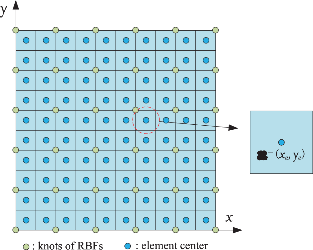
Figure 1: An example of the design domain with 10 × 10 finite elements and 6 × 6 RBFs

Several figures of two single stiffeners with different thicknesses and widths are displayed in Fig. 2. Fig. 2a indicates a schematic of the projection function Eq. (10) with η=0.1 and η=0.2, i.e., the widths of the two single stiffeners are respectively set as 2η=0.2,2η=0.4. Figs. 2b and 2c show the cross sections of the two single stiffeners, where the thickness constant in Eq. (8) is set to 0.5. Figs. 2d and 2e show the two-dimensional (2D) and three-dimensional (3D) models combined with the two stiffeners, noting that the intensity of the colors depends on the thickness of the stiffener in the 2D model.

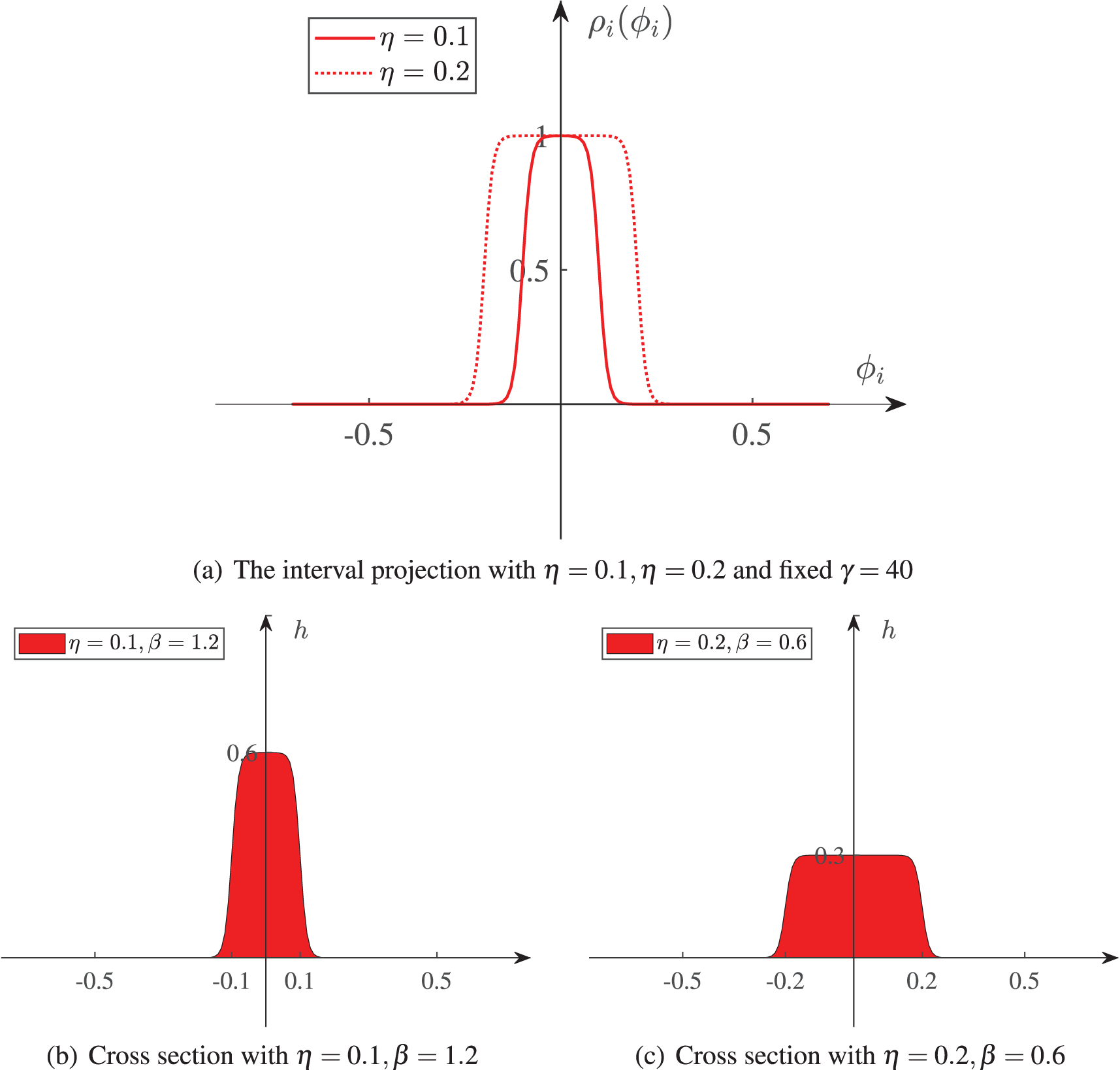
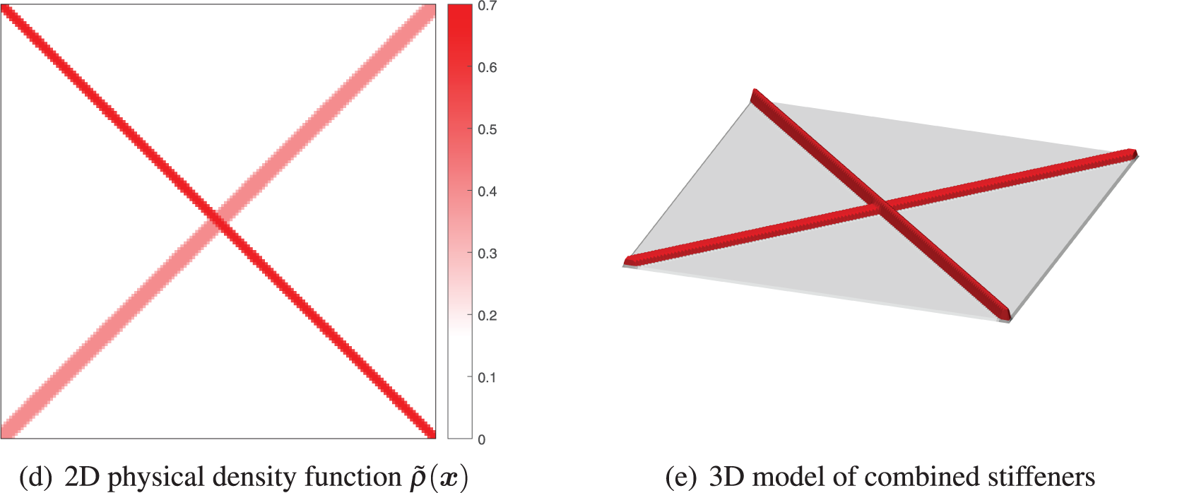
Figure 2: Several diagrams of the stiffener with separate thickness and width, and the thickness constant is set as 0.5, i.e., h=0.5β. (a) the interval projection with different widths; (b) the cross section of the stiffener with η=0.1,β=1.2; (c) the cross section of the stiffener with η=0.2,β=0.6; (d) and (e) 2D, 3D models of the physical density function ρ~(x) combined by the above two stiffeners

3  Definition of Constraints for Stiffeners

3.1 Constraint of Uniform Width

In most cases, the width of each single stiffener is expected to be uniform. Accordingly, the constraint designed to keep the width to be uniform [33] is still used in this paper. It is realized by ensuring the gradient norm of all the level sets to be equal to 1 in each element. In such circumstances, the width of each stiffener is determined by the projection parameter ηi, i.e., the width of each stiffener is approximately 2ηi.

The gradient norm of the i-th level set function ϕi(xe) is given by

‖∇ϕi(x)‖=(∑k=1mαik∂φ∂x(x,qk))2+(∑k=1mαik∂φ∂y(x,qk))2(16)

where ∂φ/∂x and ∂φ/∂y based on Eq. (14) are calculated as [33]

∂φ∂x(x,qk)=−20⋅r(x,qk)⋅(1−r(x,qk))+3∂r∂x(x,qk)(17)

∂φ∂y(x,qk)=−20⋅r(x,qk)⋅(1−r(x,qk))+3∂r∂y(x,qk)(18)

To realize the value of the gradient norm to be equal to 1, the width constraint similar to those in [33,34], is designed by

deϕi=(‖∇ϕi(xe)‖−1)2≤ξi,e=1…n, i=1…L(19)

Considering the issue of computational efficiency due to the large number of elements, the p-norm method [17] is adopted here as

gϕi=(∑e=1n[deϕi]p2)1/p2≤ξi(20)

where ξi is the upper bound of the i-th stiffener for constraint; p2>0 is the p-norm congregate parameter.

3.2 Constraint of the Stiffener Minimum Spacing

Considering the fabrication constraint on the stiffener spacing, the minimum spacing between the adjacent stiffeners must be controlled. Based on the gradient norm constraint, the spacing distance in the xy-plane is equal to the height difference in the z-direction. Accordingly, the spacing between the i + 1-th and the i-th stiffeners in e-th element is defined as follows:

sie=ϕi+1(xe)−ϕi(xe)(21)

In order to find the minimum spacing between the two adjacent stiffeners, the p-norm method [17] is used here as

si=[∑e=1n[ϕi+1(xe)−ϕi(xe)]−p3]−1/p3(22)

Further, for the two adjacent level sets as seen in Fig. 3, the spacing is calculated as ηi+1+ηi when the two corresponding stiffeners are exactly in contact. So, the minimum spacing between the i-th and i + 1-th stiffeners should be rewritten as

si=[∑e=1n[ϕi+1(xe)−ϕi(xe)]−p3]−1/p3−(ηi+ηi+1)≥s0(23)

where the s0 is the minimum required spacing.

Figure 3: A schematic example of the adjacent level sets when the corresponding stiffeners are just in contact

3.3 Constraint of Volume

In order to make good use of the material as in most optimization problems, the constraint on the stiffening material volume is defined as

V=∑e=1nρ~(xe)Aehs≤V¯(24)

where xe is the e-th element center; V¯ is the maximal allowed volume of the stiffeners; Ae denotes the area at e-th element; hs denotes the base thickness of the stiffeners.

4  Optimization Design and Sensitivity Analysis

4.1 Definition of the Design Problem

In the present study, the maximization of the critical buckling load factor is seen as the objective to be optimized; the expansion coefficients of the CS-RBFs αik, thickness variables βi and width variables ηi are the design variables. So the optimization design problem is given by

minαik,βi,ηiJ=−λ1 s.t. (K−λ1G)φ1=0αmin≤αik≤αmaxβmin≤βi≤βmaxηmin≤ηi≤ηmaxV≤V¯gϕi≤ξiSi=s0−si≤0(25)

where λ1 is the critical buckling load factor; φ1 denotes the eigenvector corresponding to the λ1; G means the global geometric stiffness matrix; K denotes the global stiffness matrix; αmin and αmax represent the lower and upper bounds of expansion coefficients αik; βmin and βmax denote the lower and upper bounds of the thickness variable βi; ηmin and ηmax mean the lower and upper bounds of the width variable ηi.

4.2 Definition of the Sensitivity Analysis

The sensitivity of theoptimization objective J for the expansion coefficients αik is defined as

∂J∂αik=−∂λ1∂αik(26)

According to Eq. (25), the partial derivative of the critical buckling load factor λ1 with respect to the αik is given by

∂λ1∂αik=1φ1TGφ1(∑e=1nφ1eT∂ke∂αikφ1e−λ1∑e=1nφ1eT∂ge∂αikφ1e)(27)

Based on Eqs. (6) and (7), we have

∂ke∂αik=∂h∂αik(3h2k1+k2+k3)(28)

∂ge∂αik=∂h∂αikg1(29)

Based on Eqs. (8)–(12), we have

∂h∂αik=∂h∂ρ~∂ρ~∂ρi∂ρi∂ϕi∂ϕi∂αik(30)

where

∂h∂ρ~=hs(31)

∂ρ~∂ρi=βip1ρi(p1−1)ρ~(1−p1)(32)

∂ρi∂ϕi=γsech2⁡[γ(ϕi+ηi)]−γsech2⁡[γ(ϕi−ηi)]tanh⁡(γηi)+tanh⁡[γ(1−ηi)](33)

∂ϕi∂αik=φ(x,qk)(34)

The sensitivity of the optimization objective J with respect to the thickness variables βi are defined as

∂J∂βi=−∂λ1∂βi(35)

∂λ1∂βi=1φ1TGφ1(∑e=1nφ1eT∂ke∂βiφ1e−λ1∑e=1nφ1eT∂ge∂βiφ1e)(36)

According to Eq. (9), we have

∂ρ~∂βi=βi(p1−1)ρip1ρ~(1−p1)(37)

The sensitivity of the optimization objective J with respect to the width variables ηi are defined as

∂J∂ηi=−∂λ1∂ηi(38)

∂λ1∂ηi=1φ1TGφ1(∑e=1nφ1eT∂ke∂ηiφ1e−λ1∑e=1nφ1eT∂ge∂ηiφ1e)(39)

According to Eqs. (10) and (11), we have

∂ρi∂ηi=γ(A−B)A=(X1 ′+X~2 ′)(X1+X3)−(X1+X~2)(X1 ′−X3 ′)(X1+X3)2B=(X1 ′−X2 ′)(X1+X3)−(X1+X2)(X1 ′−X3 ′)(X1+X3)2(40)

where

X1=tanh⁡(γηi), X3=tanh⁡[γ(1−ηi)]X2=tanh⁡[γ(ϕi−ηi)], X~2=tanh⁡[γ(ϕi+ηi)]X ′=1−X2(41)

According to Eq. (24), the sensitivity of the volume constraint V with respect to the design variable αik, βi and ηi are defined as

∂V∂αik=∑e=1n∂ρ~∂ρi∂ρi∂ϕi∂ϕi∂αikAehs(42)

∂V∂βi=∑e=1n∂ρ~∂βiAehs(43)

∂V∂ηi=∑e=1n∂ρ~∂ρi∂ρi∂ηiAehs(44)

The sensitivity of the gradient constraint gϕi with respect to the expansion coefficients αik based on Eq. (20), is given by

∂gϕi∂αik=gϕi(1−p2)∑e=1n(deϕi)(p2−1)∂deϕi∂αik(45)

According to Eqs. (16)–(19), we have

∂deϕi∂αik=2(1−1‖∇ϕi‖)[(∑j=1mαij∂φj∂x)∂φk∂x+(∑j=1mαij∂φj∂y)∂φk∂y](46)

The sensitivity of the minimum spacing constraint Si with respect to the expansion coefficients α(i+1)k, αik based on Eqs. (23) and (12), are given by

∂Si∂α(i+1)k=−(∑e=1NΔϕie−p3)−1p3−1⋅∑e=1N[Δϕie−p3−1φ(xe,qk)](47)

∂Si∂αik=(∑e=1NΔϕie−p3)−1p3−1⋅∑e=1N[Δϕie−p3−1φ(xe,qk)](48)

∂Si∂η(i+1)=1(49)

∂Si∂ηi=1(50)

where

Δϕie=ϕi+1(xe)−ϕi(xe)(51)

For most gradient-based optimization algorithms, sensitivity determines their search direction. Consequently, after obtaining all sensitivities, the Method of Move Asymptote (MMA) [35] is employed by substituting the objective function value, constraint function values, and their respective sensitivities. This computation yields updated design variables, including the expansion coefficient for the parameterized level set function, as well as thickness and width variables for the stiffeners.

4.3 Optimization Process Summary

The optimization process mainly consists of several steps: defining the design domain, mesh partition, and boundary conditions; initializing the level set function and radical basis function; conducting finite element analysis; Solving the characteristic equation to obtain the eigenvalues; performing sensitivity analysis; and updating variables. Theses steps are discussed in detail one by one as follows:

Step 1: Define the design domain, partition the design domain for finite element meshing, select the nodes for RBFs, and impose the boundary conditions.

Step 2: Based on the shape requirements of the reinforcing bars, the parameters for the expansion coefficient and threshold projection interval in the level set function are defined. The initial thickness variables are all set to 1.

Step 3: Calculate the thickness of each element and determine the stiffness matrix and geometric stiffness matrix for each individual element. Combine these to form the overall stiffness matrix and overall geometric stiffness matrix.

Step 4: Solve for eigenvalues and eigenvectors based on the characteristic equation.

Step 5: Compute the sensitivity of the objective function and constraint functions with respect to the design variables.

Step 6: Based on sensitivity information, utilize the MMA (Method of Moving Asymptotes) algorithm using gradient-based optimization to update the design variables.

Step 7: Repeat steps 3 through 6 until the iteration termination criteria are met.

5  Numerical Examples

In this section, the effectiveness of the proposed method is validated by several examples, akin to those found in other studies [8,10,36,37]. The Poisson’s ratio is set as 0.3 and the Young’s modulus of material is set as 200 GPa. The thickness constants of the stiffeners and substructure are respectively set as hs=0.5 and hb=0.1. The finite element number is set as 150×150. RBF knots are evenly distributed over all structure design domain, with a number of RBF knots 40×40 and a support radius ds=4.5 in Eq. (15). The parameter in Eq. (11) is set as γ=40. The bounds on the design variables αik are required as αmin=−50,αmax=50. And the parameters p1=8,p2=8,p3=10.

The optimization convergence criterion is given by

Cerr=|∑j=15|Ck−j+1−Ck−5−j+1||∑j=15Ck−j+1≤δc(52)

where convergence condition δc=1%; k is the current iteration steps; the maximal iteration steps is set as 500, and the optimization will end up if k exceeds it.

5.1 Example 1

The boundary conditions of the first example is given as Fig. 4. The substrate is a square plate (10 mm×10 mm), the left side and the right side of which are simply supported. And there is an axial load F=1 N/mm distributed uniformly over the left short edge in x direction, and on the right side. The parameters ξi in Eq. (20) are set as 0.08. The thickness variables βi are set as 1 initially, with bounds of 0.6≤βi≤1.2. And the widths of all stiffeners are initially set as 2η=0.2, and bounds of η are set as 0.09≤ηi≤0.11. The minimum stiffener spacing is set as s0=0.1.

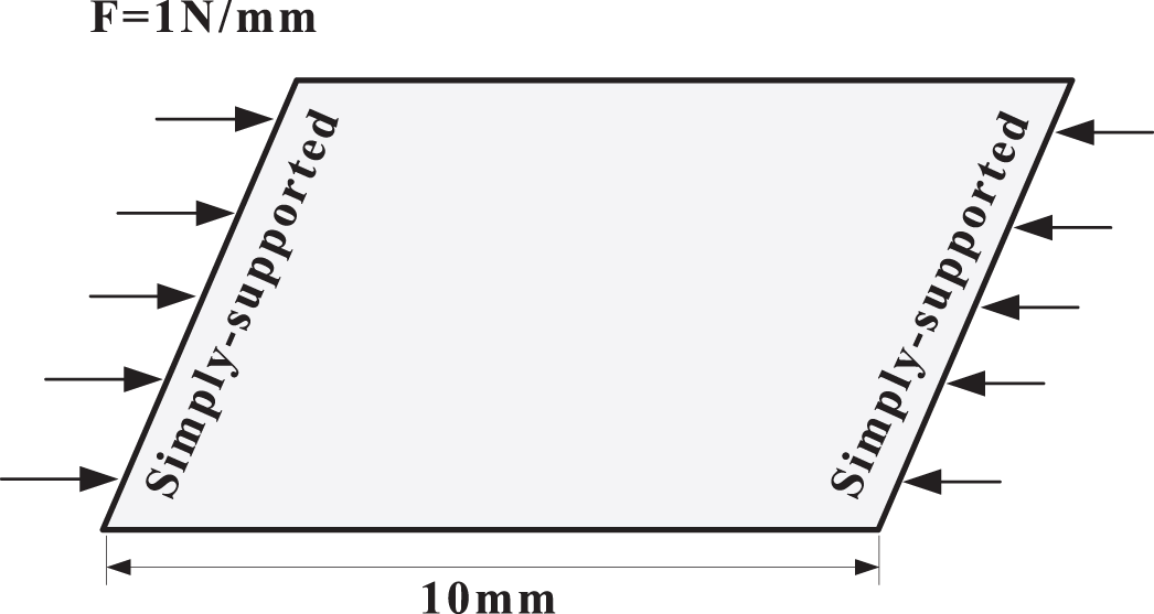
Figure 4: Design domain and boundary conditions of the first example

In this example, the optimizations using different methods are compared, that is, whether the shape and cross section are optimized simultaneously. As shown in Fig. 5, all the designs are displayed with two-dimensional (2D) and three-dimensional (3D) modality for more details, where the color intensity depends on the thickness of the stiffener. In Figs. 5c and 5d, the optimized design with cross sections has changed the thickness and width of each stiffener, indicating that material utilization could be improved by weakening the low-intensity stiffeners and strengthening the high-intensity stiffeners. Furthermore, the optimized design with both the shape and cross section is shown in Fig. 5e, where the stiffeners are optimized not only on the section, but also the shape in unison, which has improved the critical buckling load factor by nearly 80.6%. Meanwhile, Fig. 6 illustrates the first modal shape of the structure, depicting the distribution of transverse normalized displacement in the structure corresponding to the critical eigenvalue, similar to [9,10].

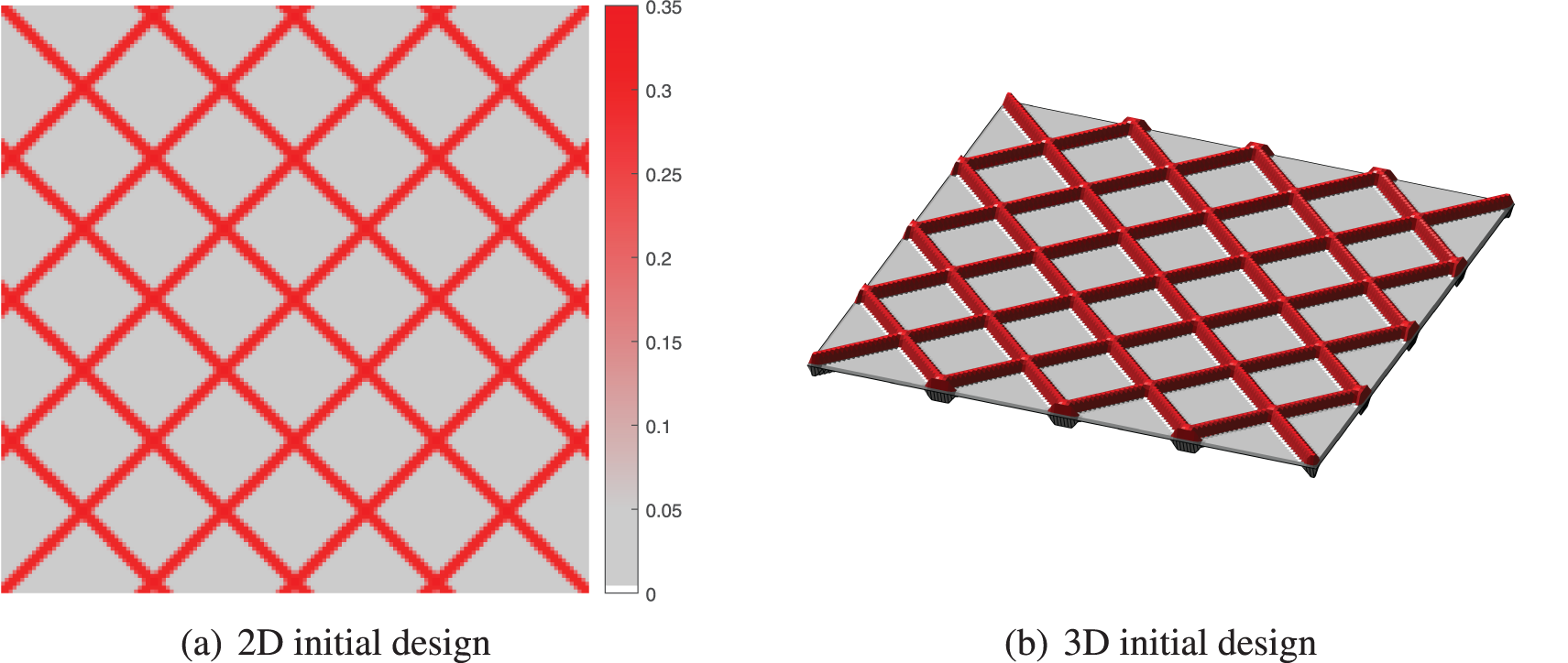
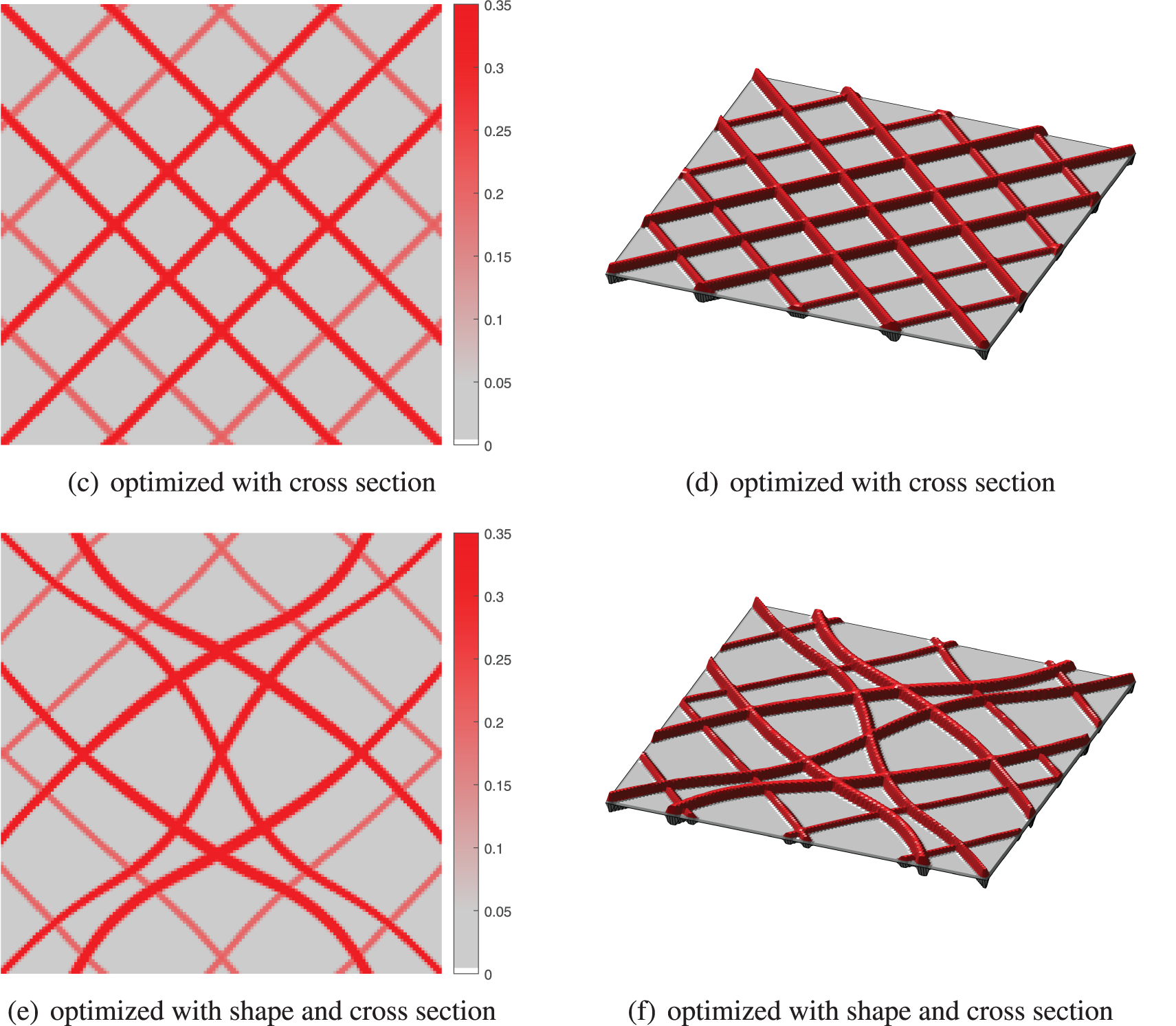
Figure 5: The optimized designs with different optimization types (The intensity of the color depends on the thickness of the stiffener in 2D, and the thicknesses in 3D have been doubled for sharper display)

Figure 6: First order buckling mode of different optimization types, (a) initial design, (b) optimized design with cross section, (c) optimized design with shape and cross section

Remarkably, both the first and second order buckling load factors are shown in Fig. 7, which proves that the optimization to maximize the critical buckling load factor is reliable as such two lines do not intersect. In addition, as seen in Figs. 8 and 9, the thickness and width of the stiffeners are optimized differently if there is a simultaneous shape change, demonstrating that the optimization of shape and cross section is collaborative rather than independent.

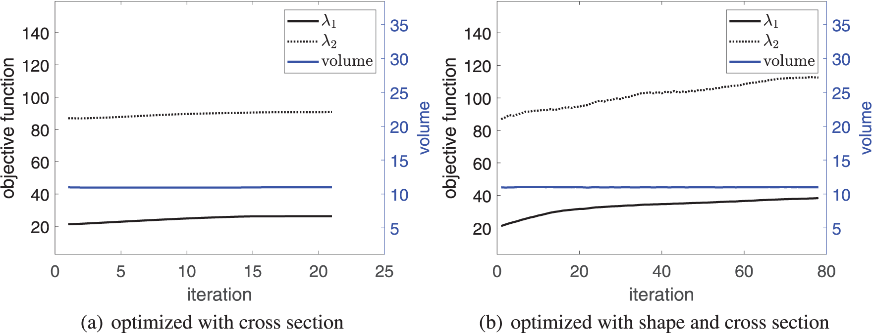
Figure 7: Convergence history of buckling load factors and volume in the first example with different optimization types, λ1,λ2 are respectively the first and second order buckling load factors. (a) λ1 is increased by 23.4%, (b) λ1 is increased by 80.6%

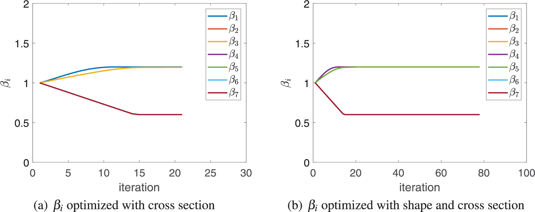
Figure 8: Convergence histories of thickness βi for the stiffeners in 45∘ direction with different optimization types. Because of symmetry, the situation of the stiffeners in the other direction is the same

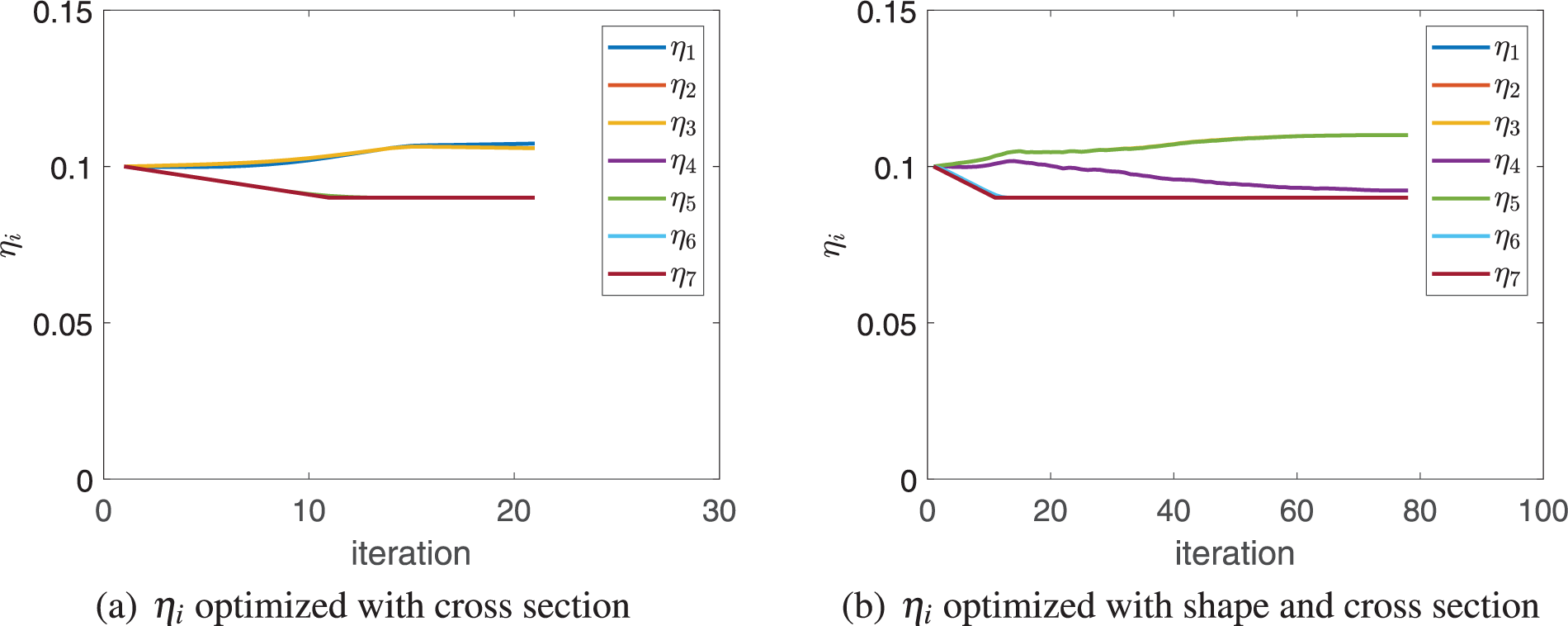
Figure 9: Convergence histories of width ηi for the stiffeners in 45∘ direction with different optimization types in the first example. Because of symmetry the situation of the stiffeners in the other direction is the same

5.2 Example 2

The boundary conditions are the same as Fig. 4. The substrate is a square plate (10 mm×10 mm), the left and right sides of which are simply supported. And there is an axial load F=1 N/mm distributed uniformly over the left short edge in x direction, and also on the right side. The parameter ξi of the stiffeners in Eq. (20) are set as 0.08. The thickness variables βi are set as 1 initially, with bounds of 0.6≤βi≤1.2. And the widths of all stiffeners are initially set as 2η=0.2, and bounds of η are set as 0.09≤ηi≤0.11.

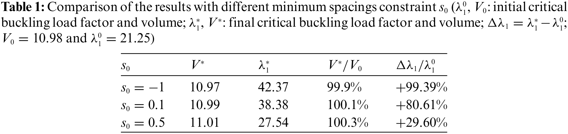
Firstly, in this example, we consider the effectiveness of the minimum spacing constraint in Eq. (23). As shown in Fig. 10, the adjacent stiffeners may be interlaced when there is not any constraint of minimum spacing (i.e., s0=−1). Conversely, the shape optimization of the stiffeners are restricted obviously due to the oversize minimum spacing (i.e., s0=0.5). Apparently, the minimum spacing constraint is effectual, and more data of the optimization are shown in Table 1.

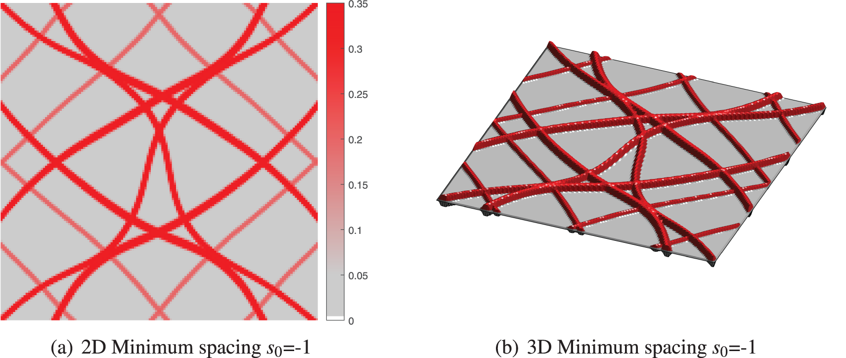
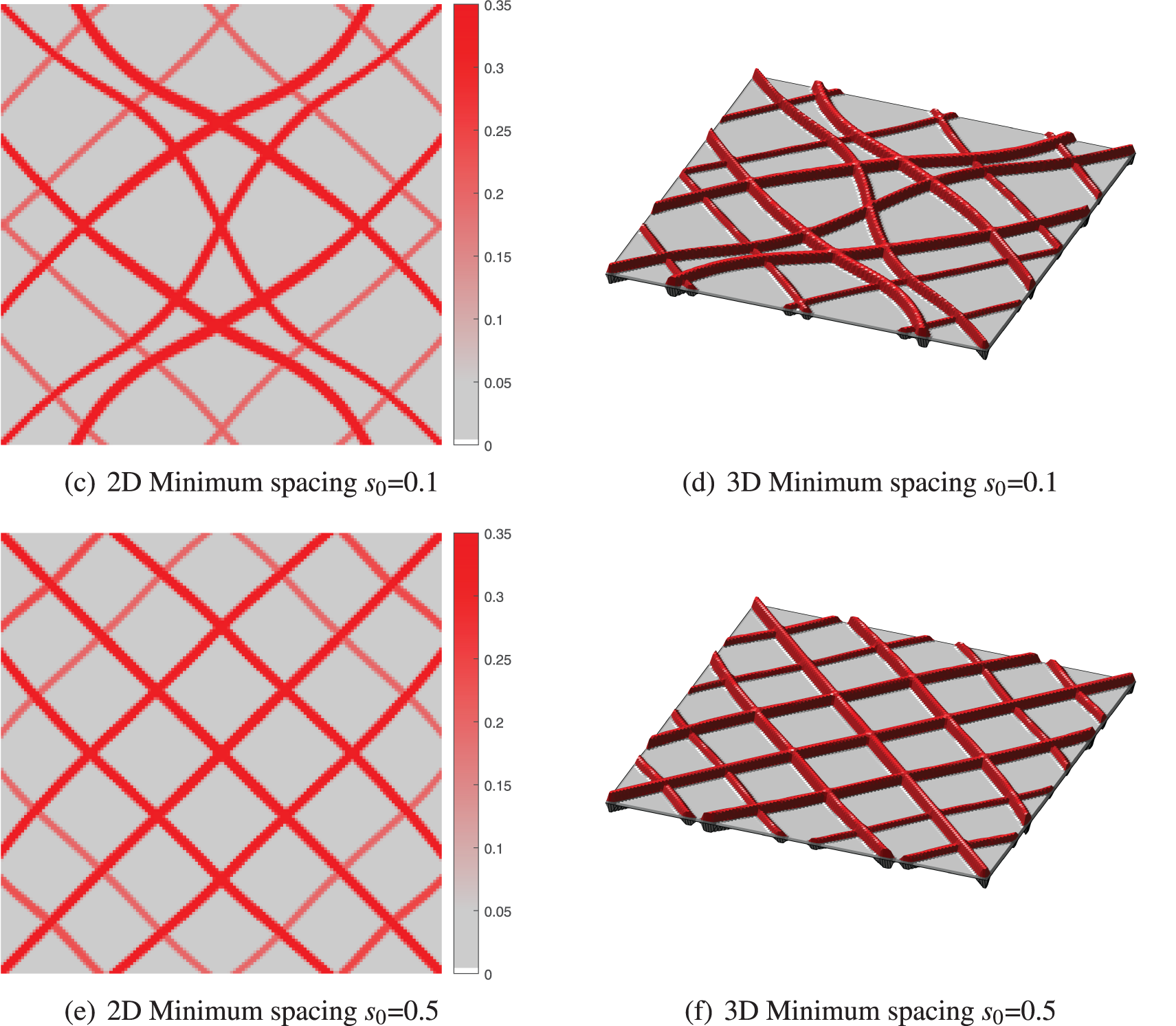
Figure 10: The optimized designs with different minimum spacings (The intensity of the color depends on the thickness of the stiffener in 2D, and the thicknesses in 3D have been doubled for sharper display)

Secondly, to account for the impact of finite element discretization, analyses were conducted using mesh sizes of 120 × 120, 150 × 150, and 180 × 180. The optimized designs of different mesh configurations are shown in Fig. 11. It can be observed that when the number of mesh elements is too low, it may impact the results of the optimization design, with the critical buckling load factor λ1 improving by only 57.2%. However, as the mesh reaches a certain quantity, the changes in the optimized results for the stiffeners become minimal and the optimization method will exhibits low dependency on the mesh, allowing for both computational efficiency and the attainment of a satisfactory optimized design. Specifically, the optimized designs for the 150 × 150 and 180 × 180 meshes remain roughly the same, with the λ1 values showing improvements of 80.6% and 83.1%, respectively.

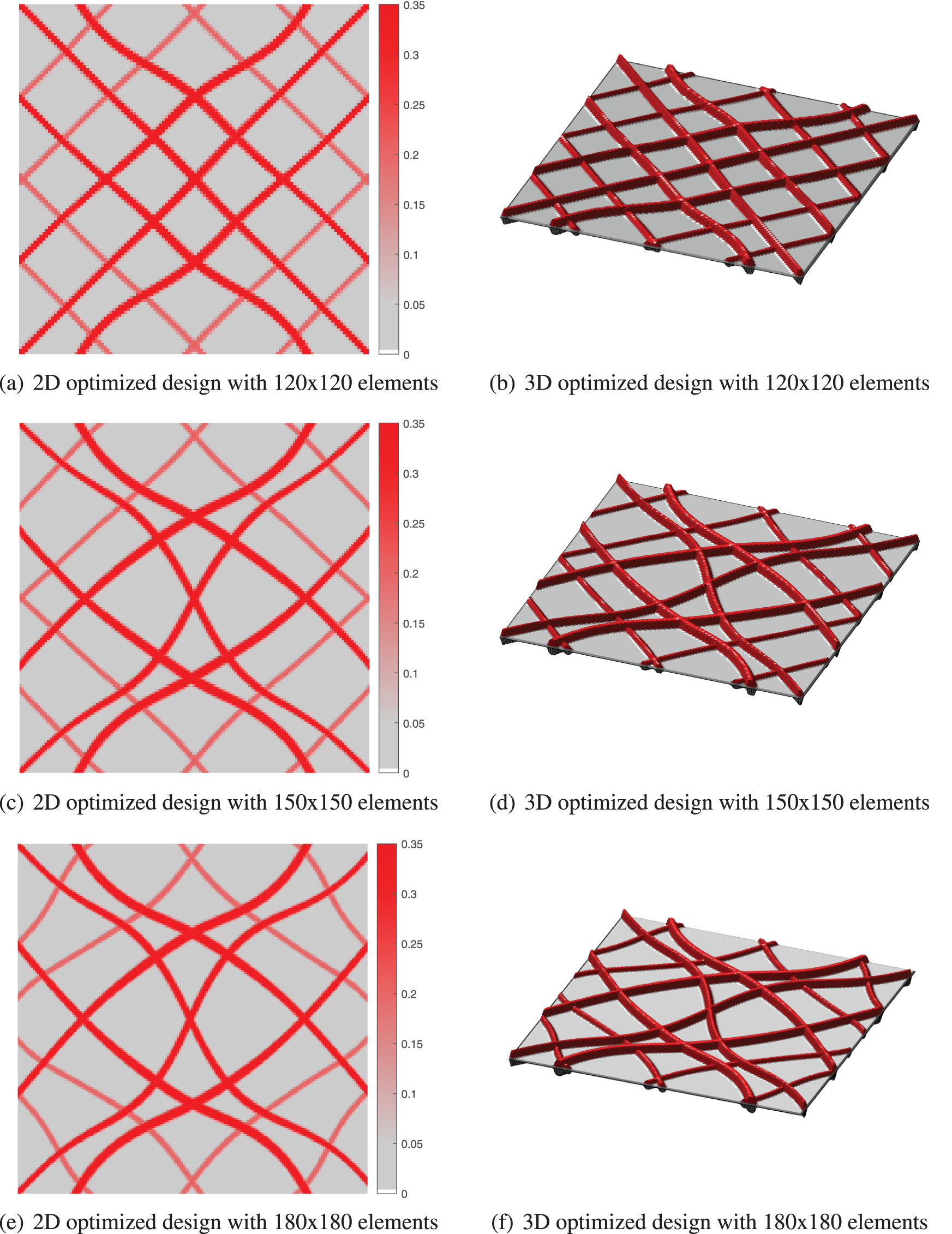
Figure 11: The optimized designs under various mesh element configurations. (a, b) λ1 is increased by 57.2%, (c, d) λ1 is increased by 80.61%, (e, f) λ1 is increased by 83.1%

5.3 Example 3

The essential boundary conditions of the third example is shown in Fig. 12. The size of the substrate is 10 mm×10 mm, the left side of which is clamped supported, while the others are free. The axial load F=1 N/mm is uniformly distributed over the right short edge in the negtive x-direction. The parameters ξi in Eq. (20) are set as 0.06. The thickness variables βi are set as 1 initially, with bounds of 0.6≤βi≤1.5. And the widths of all stiffeners are initially set as 2η=0.2, and bounds of η are set as 0.09≤ηi≤0.11. The minimum stiffener spacing is set as s0=0.1.

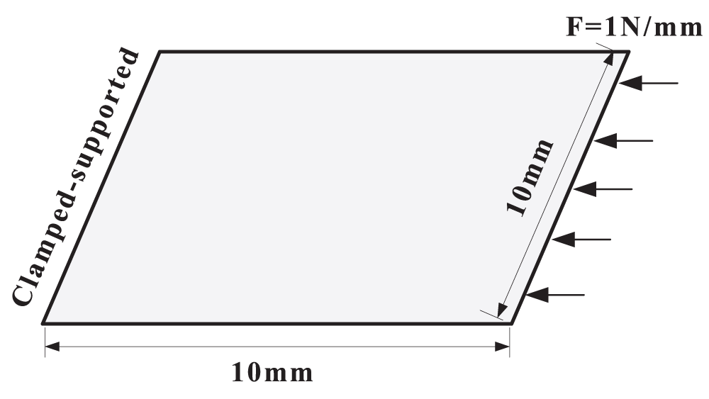
Figure 12: Design domain and boundary conditions of the third example

In this example, with the same distribution of stiffeners as in Fig. 5a, the optimization is performed with different admissible volumes V¯ as shown in Fig. 13. The critical buckling load factor in Fig. 14 is improved by different percents even when the material is reduced. As the volume of material gradually decreases, the low-intensity stiffeners are weakened further as the material focuses on the primary stiffeners, taking into account the contribution to structural stability. One can be seen in Figs. 15 and 16, the thickness and width of the stiffeners that contribute more to the stability of the structure are enhanced by the weakening of the other stiffeners. Finally, Fig. 17 illustrates the first modal shape of the structure, depicting the distribution of transverse normalized displacement in the structure corresponding to the critical eigenvalue, similar to [9,10].

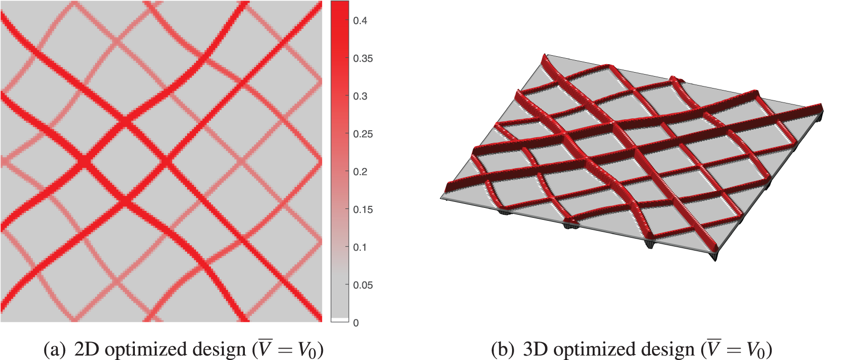
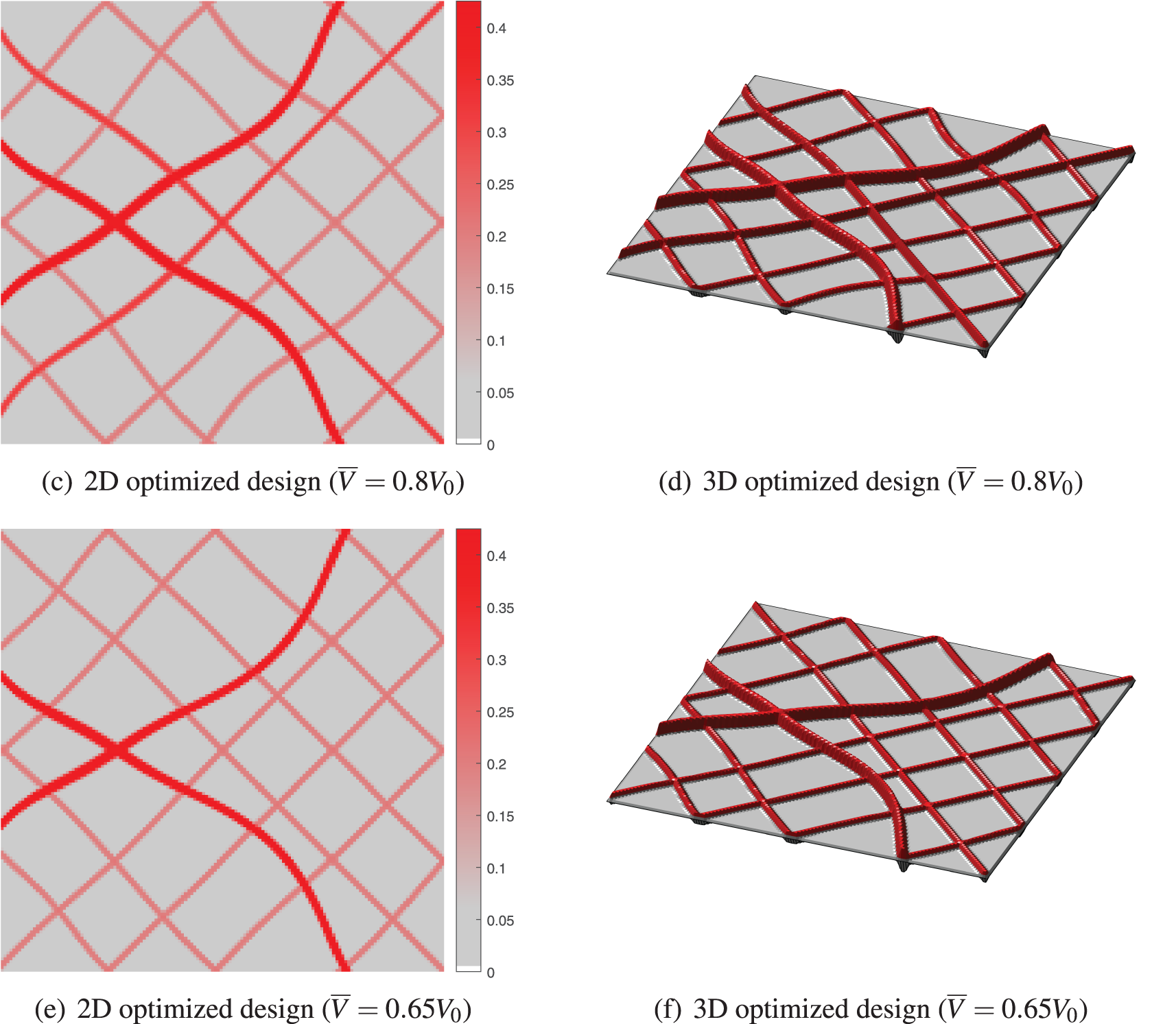
Figure 13: The optimized designs with different admissible volumes, as the same initial design as in Example 1 (The intensity of the color depends on the thickness of the stiffener in 2D, and the thicknesses in 3D have been doubled for sharper display)

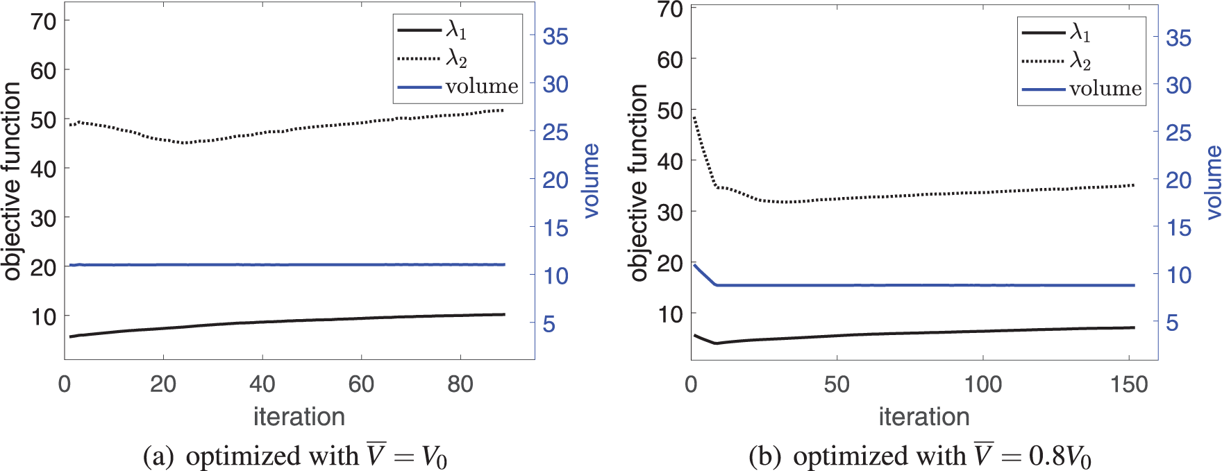
Figure 14: Convergence history of buckling load factors and volume in the second example with different admissible volumes, λ1,λ2 are respectively the first and second order buckling load factors. (a) λ1 is increased by 79.89%, (b) λ1 is increased by 25.40%

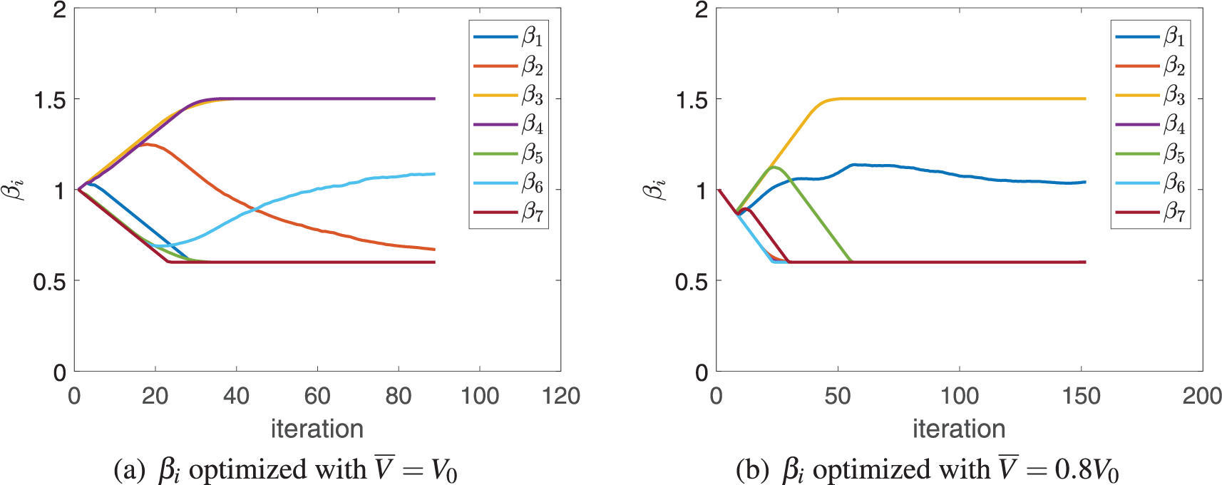
Figure 15: Convergence histories of thickness βi for the stiffeners in 45∘ direction with different admissible volumes. Because of symmetry the situation of the stiffeners in the other direction is the same

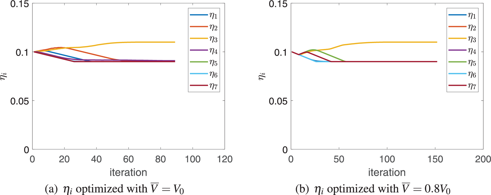
Figure 16: Convergence histories of width ηi for the stiffeners in 45∘ direction with different admissible volumes. Because of symmetry the situation of the stiffeners in the other direction is the same

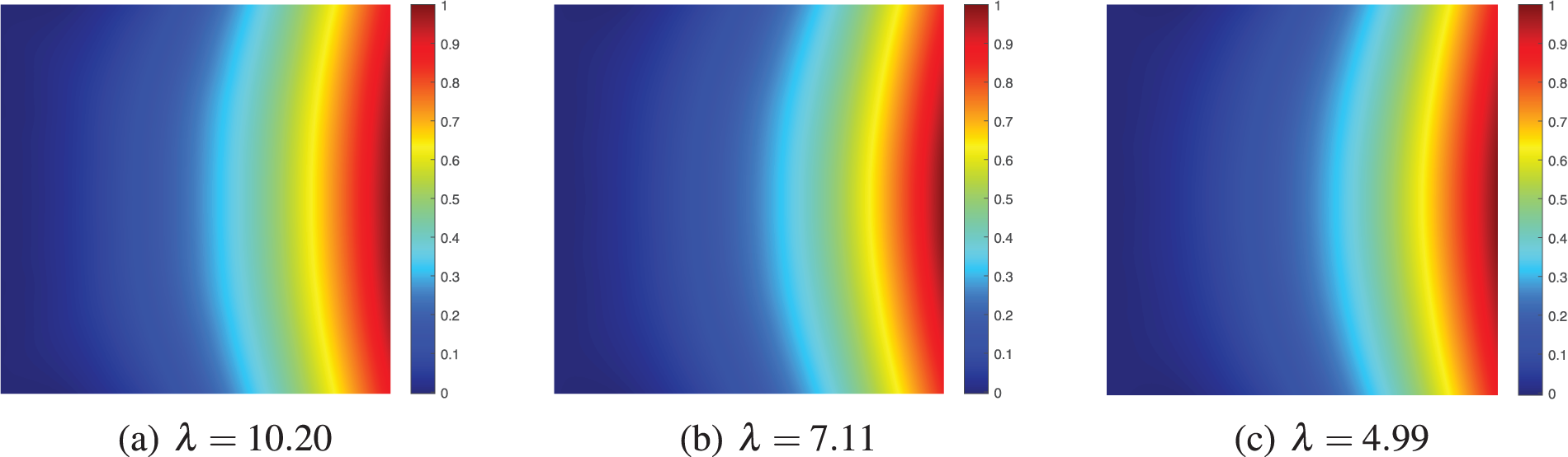
Figure 17: First order buckling mode with different admissible volumes, (a) optimized with V¯=V0, (b) optimized with V¯=0.8V0, (c) optimized with V¯=0.65V0

Compared to the first example, the upper bound on the thickness variable is raised, and during the optimization one can see that the material is still used to reinforce several main stiffeners up to the upper limit, ensuring the strength of the structure. Further, if the material is reduced by even less, the bounds on the thickness and width can be lowered to accommodate the material variations.

6  Conclusions

A novel buckling optimization method of curved grid stiffeners is proposed in this paper, where the shape and cross section (including thickness and width) of each stiffener can be optimized in a synchronous and flexible manner to improve the critical buckling load factor of the stiffened structure.

Based on the level set based density method proposed in the previous study [16], the grid stiffeners are composed of different single stiffeners projected by the corresponding level set functions. As an enhancement, the thickness and width of each stiffener are designed as unrestricted variables. This allows the material to freely redistribute from a low-intensity stiffener to a high-intensity one. In other words, the width and thickness of the stiffener are adjusted based on their contribution to structural stability, either being enhanced or weakened. Additionally, the spacing between neighboring stiffeners is effectively controlled for manufacturing considerations. All these advancements have been successfully demonstrated in the buckling optimization.

Acknowledgement: The authors sincerely appreciate the insightful comments from the reviewers and also gratefully thank Krister Svanberg for providing the MMA codes.

Funding Statement: The present research works are supported by the National Natural Science Foundation of China (Grant Nos. 51975227 and 12272144).

Author Contributions: The authors confirm contribution to the paper as follows: study conception and design: Zhuo Huang, Qi Xia; data collection: Ye Tian; analysis and interpretation of results: Zhuo Huang, Yifan Zhang, Tielin Shi; draft manuscript preparation: Zhuo Huang, Qi Xia. All authors reviewed the results and approved the final version of the manuscript.

Availability of Data and Materials: None.

Conflicts of Interest: The authors declare that they have no conflicts of interest to report regarding the present study.

References

1. Jadhav, P., Mantena, P. R. (2007). Parametric optimization of grid-stiffened composite panels for maximizing their performance under transverse loading. Composite Structures, 77(3), 353–363. [Google Scholar]

2. Zhu, J. H., Zhang, W. H., Xia, L. (2016). Topology optimization in aircraft and aerospace structures design. Archives of Computational Methods in Engineering, 23(4), 595–622. [Google Scholar]

3. Ma, H., Jiao, P., Li, H., Cheng, Z., Chen, Z. (2023). Buckling analyses of thin-walled cylindrical shells subjected to multi-region localized axial compression: Experimental and numerical study. Thin-Walled Structures, 183, 110330. [Google Scholar]

4. Kapania, R. K., Li, J., Kapoor, H. (2005). Optimal design of unitized panels with curvilinear stiffeners. AIAA 5th ATIO and the AIAA 16th Lighter-than-Air Systems Technology Conference and Balloon Systems Conference, vol. 3, pp. 1708–1737. Arlington, Virgina. [Google Scholar]

5. Zhao, W., Kapania, R. K. (2016). Buckling analysis of unitized curvilinearly stiffened composite panels. Composite Structures, 135, 365–382. [Google Scholar]

6. Tamijani, A. Y., Kapania, R. K. (2015). Chebyshev-ritz approach to buckling and vibration of curvilinearly stiffened plate. Aiaa Journal, 50(5), 1007–1018. [Google Scholar]

7. Townsend, S., Kim, H. A. (2019). A level set topology optimization method for the buckling of shell structures. Structural and Multidisciplinary Optimization, 60(5), 1783–1800. [Google Scholar]

8. Luo, Y., Zhan, J. (2020). Linear buckling topology optimization of reinforced thin-walled structures considering uncertain geometrical imperfections. Structural and Multidisciplinary Optimization, 62(4), 3367–3382. [Google Scholar]

9. Wang, D., Abdalla, M. M. (2015). Global and local buckling analysis of grid-stiffened composite panels. Composite Structures, 119, 767–776. [Google Scholar]

10. Wang, D., Abdalla, M. M., Zhang, W. (2017). Buckling optimization design of curved stiffeners for grid-stiffened composite structures. Composite Structures, 159, 656–666. [Google Scholar]

11. Zheng, Q., Jiang, D., Huang, C., Shang, X., Ju, S. (2015). Analysis of failure loads and optimal design of composite lattice cylinder under axial compression. Composite Structures, 131, 885–894. [Google Scholar]

12. Lopatin, A. V., Morozov, E. V. (2015). Buckling of the composite sandwich cylindrical shell with clamped ends under uniform external pressure. Composite Structures, 122, 209–216. [Google Scholar]

13. Ghazijahani, T. G., Jiao, H., Holloway, D. (2015). Longitudinally stiffened corrugated cylindrical shells under uniform external pressure. Journal of Constructional Steel Research, 110, 191–199. [Google Scholar]

14. Singh, K., Kapania, R. K. (2021). Accelerated optimization of curvilinearly stiffened panels using deep learning. Thin-Walled Structures, 161(3), 107418. [Google Scholar]

15. Bostan, B., Kusbeci, M., Cetin, M., Kirca, M. (2023). Buckling performance of fuselage panels reinforced with voronoi-type stiffeners. International Journal of Mechanical Sciences, 240, 107923. [Google Scholar]

16. Huang, Z., Tian, Y., Yang, K., Shi, T., Xia, Q. (2023). Shape and generalized topology optimization of curved grid stiffeners through the level set based density method. Journal of Mechanical Design, 145(11), 111704. https://doi.org/10.1115/1.4063093 [Google Scholar] [CrossRef]

17. Le, C., Norato, J., Bruns, T., Ha, C., Tortorelli, D. (2010). Stress-based topology optimization for continua. Structural and Multidisciplinary Optimization, 41(4), 605–620. [Google Scholar]

18. Ma, H., Gao, X. L., Reddy, J. (2011). A non-classical mindlin plate model based on a modified couple stress theory. Acta Mechanica, 220(1–4), 217–235. [Google Scholar]

19. Batista, M. (2010). An elementary derivation of basic equations of the reissner and mindlin plate theories. Engineering Structures, 32(3), 906–909. [Google Scholar]

20. Liu, H., Chen, L., Shi, T., Xia, Q. (2022). M-vcut level set method for the layout and shape optimization of stiffeners in plate. Composite Structures, 293, 115614. [Google Scholar]

21. Wodesenbet, E., Kidane, S., Pang, S. S. (2003). Optimization for buckling loads of grid stiffened composite panels. Composite Structures, 60(2), 159–169. [Google Scholar]

22. Wang, J. T. S., Hsu, T. M. (1985). Discrete analysis of stiffened composite cylindrical shells. AIAA Journal, 23(11), 1753–1761. [Google Scholar]

23. Zhang, W. H., Zhou, Y., Zhu, J. H. (2017). A comprehensive study of feature definitions with solids and voids for topology optimization. Computer Methods in Applied Mechanics and Engineering, 325, 289–313. [Google Scholar]

24. Savine, F., Irisarri, F. X., Julien, C., Vincenti, A., Guerin, Y. (2021). A component-based method for the optimization of stiffener layout on large cylindrical rib-stiffened shell structures. Structural and Multidisciplinary Optimization, 64(4), 1843–1861. [Google Scholar]

25. Bendse, M. P. (1989). Optimal shape design as a material distribution problem. Structural Optimization, 1(4), 193–202. [Google Scholar]

26. Rozvany, G. I. N., Zhou, M., Birker, T. (1992). Generalized shape optimization without homogenization. Structural Optimization, 4(3), 250–254. [Google Scholar]

27. Wang, F. W., Lazarov, B. S., Sigmund, O. (2011). On projection methods, convergence and robust formulations in topology optimization. Structural and Multidisciplinary Optimization, 43(6), 767–784. [Google Scholar]

28. Clausen, A., Aage, N., Sigmund, O. (2015). Topology optimization of coated structures and material interface problems. Computer Methods in Applied Mechanics and Engineering, 290, 524–541. [Google Scholar]

29. Wang, S., Wang, M. (2006). Structural shape and topology optimization using an implicit free boundary parametrization method. Computer Modeling in Engineering & Sciences, 13(2), 119–147. [Google Scholar]

30. Luo, Z., Tong, L., Wang, M. Y., Wang, S. (2007). Shape and topology optimization of compliant mechanisms using a parameterization level set method. Journal of Computational Physics, 227(1), 680–705. [Google Scholar]

31. Wang, Y., Luo, Z., Kang, Z., Zhang, N. (2015). A multi-material level set-based topology and shape optimization method. Computer Methods in Applied Mechanics and Engineering, 283, 1570–1586. [Google Scholar]

32. Wei, P., Li, Z. Y., Li, X. P., Wang, M. Y. (2018). An 88-line matlab code for the parameterized level set method based topology optimization using radial basis functions. SStructural and Multidisciplinary Optimization, 58(2), 831–849. [Google Scholar]

33. Yang, K., Tian, Y., Shi, T., Xia, Q. (2022). A level set based density method for optimizing structures with curved grid stiffeners. Computer-Aided Design, 153, 103407. [Google Scholar]

34. Jiang, L., Chen, S. K. (2017). Parametric structural shape & topology optimization with a variational distance-regularized level set method. Computer Methods in Applied Mechanics and Engineering, 321, 316–336. [Google Scholar]

35. Svanberg, K. (1987). The method of moving asymptotes-a new method for structural optimization. International Journal for Numerical Methods in Engineering, 24(2), 359–373. [Google Scholar]

36. Wang, W., Ye, H., Li, Z., Sui, Y. (2023). Topology optimization for disc structures with buckling and displacement constraints. Engineering Optimization, 55(1), 35–52. [Google Scholar]

37. Lindgaard, E., Lund, E. (2011). Optimization formulations for the maximum nonlinear buckling load of composite structures. Structural and Multidisciplinary Optimization, 43(5), 631–646. [Google Scholar]