
 Submit a Paper
 Propose a Special lssue
 Open Access
ARTICLE

Fatigue Crack Propagation Law of Corroded Steel Box Girders in Long Span Bridges
1 Key Laboratory of Concrete and Prestressed Concrete Structures of Ministry of Education, School of Civil Engineering, Southeast University, Nanjing, 211189, China
2 Jiangsu Provincial Engineering Construction Standard Station, Nanjing, 210036, China
* Corresponding Author: Ying Wang. Email:
Computer Modeling in Engineering & Sciences 2024, 140(1), 201-227. https://doi.org/10.32604/cmes.2024.046129
Received 19 September 2023; Accepted 22 January 2024; Issue published 16 April 2024
 View Full Text
 Download PDF
Abstract
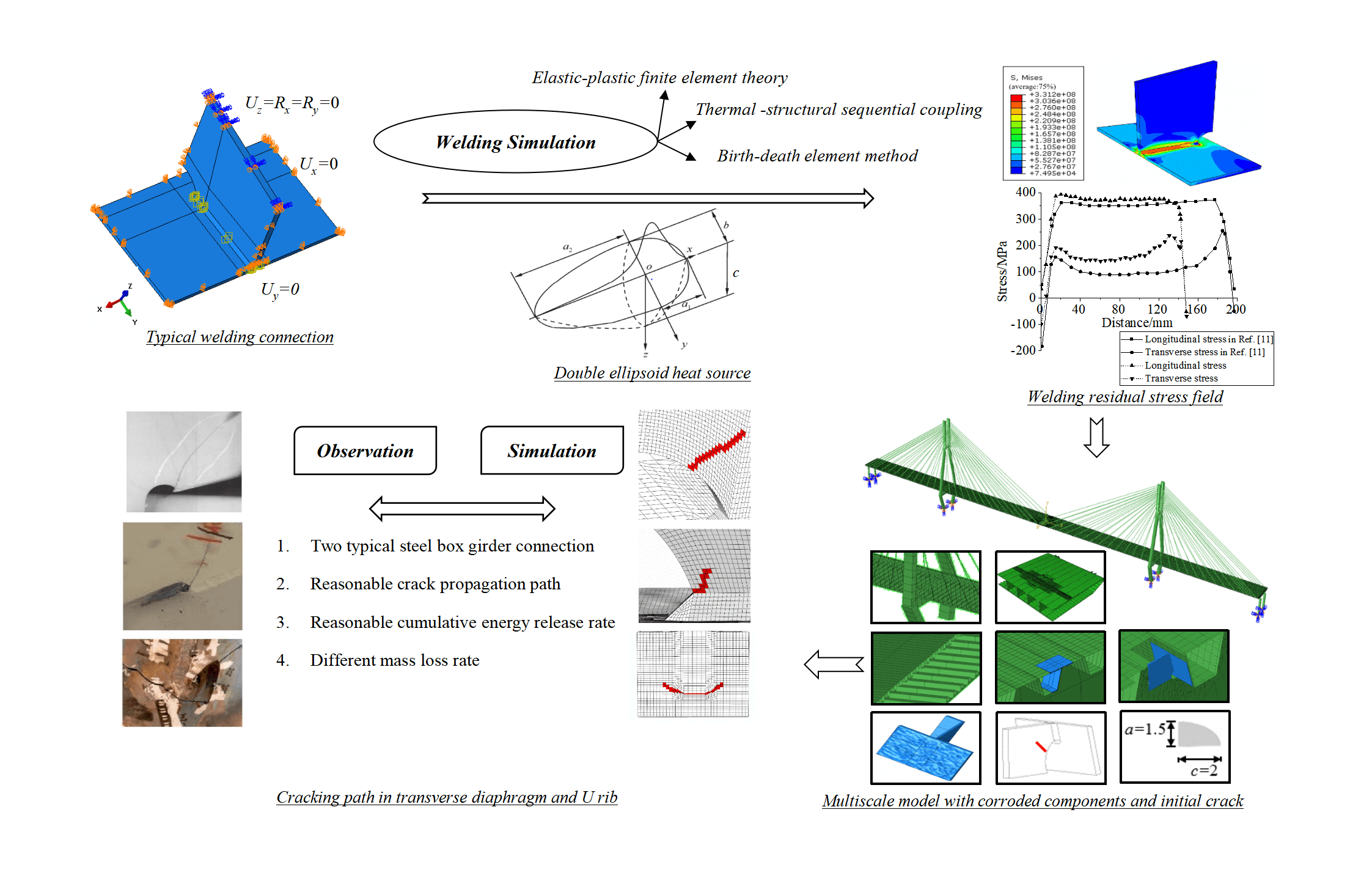
In order to investigate the fatigue performance of orthotropic anisotropic steel bridge decks, this study realizes the simulation of the welding process through elastic-plastic finite element theory, thermal-structural sequential coupling, and the birth-death element method. The simulated welding residual stresses are introduced into the multiscale finite element model of the bridge as the initial stress. Furthermore, the study explores the impact of residual stress on crack propagation in the fatigue-vulnerable components of the corroded steel box girder. The results indicate that fatigue cracks at the weld toe of the top deck, the weld root of the top deck, and the opening of the transverse diaphragm will not propagate under the action of a standard vehicle load. However, the inclusion of residual stress leads to the propagation of these cracks. When considering residual stress, the fatigue crack propagation paths at the weld toe of the transverse diaphragm and the U-rib weld toe align with those observed in actual bridges. In the absence of residual stress, the cracks at the toe of the transverse diaphragm with a 15% mass loss rate are categorized as type I cracks. Conversely, when residual stress is considered, these cracks become I-II composite cracks. Residual stress significantly alters the cumulative energy release rate of the three fracture modes. Therefore, incorporating the influence of residual stress is essential when assessing the fatigue performance of corroded steel box girders in long-span bridges.Graphic Abstract
Keywords
Bridge steel box girders consist of a top deck, bottom deck, inclined webs, transverse diaphragms, longitudinal transverse diaphragms, and U-shaped longitudinal ribs. They are widely used in long-span bridges both domestically and internationally, owing to their lightweight and superior overall mechanical performance. The welding process, involving multiple plates, invariably leads to residual stresses in the orthotropic steel bridge panels of steel box girders. Residual tensile stresses near the weld center can approach the steel’s yield strength, markedly affecting fatigue performance. Welded components are susceptible to the initiation of fatigue cracks and other welding defects. These cracks tend to propagate unstably under the repeated loading from vehicular traffic. Moreover, the bridge, exposed to prolonged humidity and rainwater, undergoes electrochemical corrosion of its steel box girder components, leading to etching pits or corroded surfaces that further accelerate fatigue cracking. Therefore, researching the fatigue performance and dynamic crack propagation behavior of corroded steel box girders is of significant practical importance and engineering application value. Additionally, exploring the impact of residual stress on crack propagation patterns is vital.
To accurately simulate the welding process, scholars both domestically and internationally have consistently advanced theoretical derivations and practical applications of the finite element method [1–4]. Yukio et al. [5] introduced the thermoelastic-plastic theory, using the finite element method to simulate complex nonlinear dynamic welding processes. Teng et al. [6] applied the birth-death element technique in ANSYS software to calculate residual stress in intricate welding processes. Cao et al. [7] performed a welding thermal coupling analysis using ABAQUS software. We [4] and others have employed ANSYS finite element analysis software to examine the top deck-longitudinal rib double-sided welding model, obtaining the welding residual stress field distribution law, and concluded that the effect of welding residual stress on a structure’s mechanical behavior is significant.
Given the prevalence of residual stresses in welded structures, accounting for their influence in both fatigue performance assessment and fatigue crack propagation analysis is essential. Gurney [8] observed that under alternating constant amplitude cyclic loading, the fatigue performance of welding joints significantly diminishes due to substantial residual tensile stress. Withers [9] found that welding residual stress can cause stress redistribution during fracture, with stress continuously changing during crack propagation. Jiang et al. [10] discovered that the impact of residual stress on fatigue life primarily appears as an increase in average stress, depending on stress redistribution, and this redistribution of residual stress is intimately linked to the fatigue fracture behavior of welds.
Current research mainly focuses on intact steel structures, with few studies addressing the fatigue crack propagation behavior of corroded steel box girders. Furthermore, the influence of residual stress on the crack propagation path and rate in corroded steel box girders is rarely explored. This study numerically simulates the entire welding process of representative welding components using ABAQUS finite element software. The welding residual stresses obtained in the U-rib-to-transverse diaphragm detail and top deck-to-U-rib detail are then used as initial stresses in the multiscale finite element model of the bridge. The static stress intensity factors at the tips of seven typical fatigue cracks in two fatigue-prone positions of corroded steel box girders under standard vehicle load, including the U-rib-to-transverse diaphragm and top deck-to-U-rib details, are studied. This research investigates the fracture properties at different welding details and the effects of varying corrosion degrees on these properties. Additionally, the extended finite element method (XFEM) is used to investigate the crack propagation paths, rates, and cumulative energy release rates in fatigue-prone regions of corroded steel box girders. This study aims to elucidate the impact of welding residual stresses on the fatigue crack propagation patterns in corroded steel box girders, considering the combined influence of these stresses and moving vehicle loads.
2 Welding Simulation of Typical Fatigue-Prone Components of Steel Box Girders
The welding procedure for steel box girders in long-span bridges represents a distinctive nonlinear transient heat transfer process. ABAQUS software constructs a finite element model for this welding analysis. This model computes the welding stress field using the thermoelastic-plastic analysis method alongside the “birth-death element method,” and implements heat-force sequential coupling.
2.1 Fundamentals of the Birth-Death Element Method
In finite element analysis, simulating the deletion or addition of units in a model is achieved through either “killing” or “activating” selected units, a technique known as the birth-death element method. The occurrence of a unit’s “birth” or “death” does not directly add or remove it from the finite element model. When applying cell “death” analysis in finite element analysis (FEA), the stiffness matrix of the targeted cell is reduced significantly. Concurrently, the unit load, mass, damping, specific heat, and other related effects of the unit marked for “killing” are nullified. Additionally, the strain of the unit is set to zero upon its “death”.
Conversely, unit “birth” analysis involves reactivating previously “killed” units, essentially reversing the “death” process. The “birth” of a unit entails its initial “killing,” followed by reactivation at the correct load step. This process involves scaling down the stiffness matrix of the previously “killed” unit to a negligible factor. Upon reactivation, the unit’s loads, mass, damping, specific heat, etc., revert to their original values.
2.2 Simulation of the Welding Process
The thermodynamic and thermophysical properties of Q345qD steel, obtained from reference [11], vary with temperature, as depicted in Fig. 1. The welding simulation demonstrates the joint between the U-rib and the transverse diaphragm. The U-rib deck, measuring 300 by 200 mm, features two symmetrically placed welding seams along both sides of the transverse diaphragm. As shown in Fig. 2a, the model specifies the cell type as C3D8RT, an eight-node thermally coupled hexahedral cell, and divides the mesh. All components outside the weld seam are hidden to streamline, treating the weld seam element as a birth-death element. Material properties for the orthotropic anisotropic steel bridge deck, consisting of Q345qD steel, are defined accordingly.

Figure 1: The thermodynamic analysis parameters of Q345 steel

Figure 2: Modeling and boundary condition setting for welding analysis
The assembly of the transverse diaphragm and U-rib models leads to the creation of an analysis step comprising three phases. ① The welding process simulates the melting of solder, akin to creating solder from nothing. In the initial removal stage (step-0), a brief duration of 1e-10 s is set under the assumption that the temperature field remains relatively unaffected by the solder’s presence. Geometric nonlinearity is activated, allowing up to 10,000 incremental steps, with a maximum permissible temperature change of 2000°C per load step. ② Python’s for-loop statement efficiently configures each birth-death element’s analysis step. Each element’s welding time is fixed at 1 s, with an initial incremental step of 0.001, a minimum of 1e-7, and a maximum of 1. The maximum temperature shift per element is capped at 2000°C. ③ A cooling phase, named ‘step-cool,’ spans 3000 s, ensuring complete cooling of the weldment to room temperature. This phase sets a maximum incremental step of 10,000, with an initial step of 0.001, a minimum of 1e-5, and a maximum of 300.
The interaction module setup includes: ① ‘Int-0,’ which rapidly deactivates the weld seam within a minuscule time frame of 1e-10 s during ‘step-0’. ② Reactivation interactions, swiftly conFig.d using a Python for-loop. ③ ‘Int-film,’ establishing surface heat exchange conditions with a heat dissipation film coefficient of 10 and an ambient temperature of 20°C. ④ ‘Int-radia,’ defining surface radiation conditions with an emissivity of 0.85 and an ambient temperature of 20°C, and setting the radiation Boltzmann constant at 5.67 × 10⁻⁸ W·(m2·°C4)−1.
Set up the load module: ① In the welding step, apply body heat flux at the weld seam position, deactivating the heat source during the cooling step. ② Boundary conditions include a fixed symmetric constraint applied around the U-rib-transverse diaphragm. This constrains y-direction displacement (Uy = 0) at the bottom of the transverse diaphragm and the U-rib. Additionally, a symmetric constraint in the z-direction is imposed at the boundary of the transverse diaphragm, constraining translational displacement (Uz = 0) in the z-direction and rotational displacements (Rx = Ry = 0) in the x- and y-directions. Furthermore, x-direction displacement (Ux = 0) is constrained on both sides of the U-rib web. ③ Establish the predefined temperature field, with room temperature set at 20°C. Use the ABAQUS user subroutine DFLUX to implement the movement of a dual ellipsoid heat source. Create job files and execute the program.
The welding simulation process for the top deck-U-rib model aligns with that of the U-rib-transverse diaphragm. The top deck model has planar dimensions of 300 × 200 mm. During thermal stress analysis, z-direction symmetric constraints (Uz = Rx = Ry = 0) are applied at the symmetric centerline of the U-rib and the top deck. Constrain y-direction translational displacement Uy = 0 on both sides of the bottom surface of the top deck; constrain displacement Ux = 0 in the x-direction at one end of the section, with the finite element model shown in Fig. 2b.
2.3 Thermoelastic-Plastic Theory
The localized application of highly concentrated transient heat inputs during the welding process can lead to significant welding stresses and distortions both before and after the entire welding procedure. Thermoelastic-plastic analysis theory is employed in the step-by-step tracking of thermal strain behavior during the welding thermal cycling process to compute thermal stress and strain. This method enables monitoring of stress-strain variations throughout the welding process, ultimately facilitating the determination of welding residual stress and deformation.
The relationship between stress and strain is shown in Eq. (1).
where
The equilibrium equation is shown in Eq. (2).
where
The solution process for thermoelastic-plastic finite element analysis involves discretizing the component into a finite number of cells. Subsequently, temperature increments, pre-calculated from the weld temperature field, are incrementally added. Upon each addition of a temperature increment, Eq. (2) is utilized to determine the displacement increment at each node, denoted as
Then, according to the stress-strain relationship Eq. (1), the stress increment of each cell can be solved to obtain
2.4 Welding Heat Source Modeling
During the welding process, the arc melts the workpiece by converting electrical energy into thermal energy, but not all converted thermal energy is used for heating the weldment. Therefore, effective thermal energy is defined as follows:
where Q is the effective thermal energy of the welding heat source;
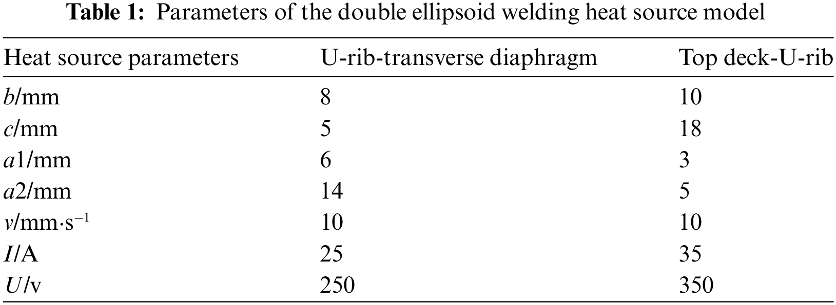
The heat source model employed for welding simulation in this paper is a double ellipsoid heat source. To capture the heating characteristics of the heat source along the depth direction of the weldment, a parameter ‘c’ is introduced to this model, as illustrated in Fig. 3. The model resembles a water droplet, with two 1/4 ellipsoids of varying sizes in the front and rear components of the welding pool. The heat source value is largest at the center position of the model, and the magnitude of the heat source value decreases inversely proportional to the distance from the center.

Figure 3: Schematic diagram of double ellipsoid heat source
The heat flux density function of a 1/4 ellipsoid in the positive half-axis of the x-axis is:
The heat flux density function of a 1/4 ellipsoid in the negative half-axis of the x-axis is:
where f1 and f2 are the energy fractions of a 1/4 ellipsoid, where f1 + f2 = 2; Q has the same physical meaning as above; v is the welding speed; a1 and a2 represent the half-axis lengths of the positive and negative half axes, respectively, with b being the half axis length in the y direction and c being the half axis length in the z-direction.
During the welding process, the temperature field is greatly influenced by the parameters of the heat source model, welding voltage, and welding current. This article makes appropriate adjustments based on reference [11], and the selected double ellipsoid heat source parameters are displayed in Table 1. By programming the ABAQUS user subroutine DFLUX, the movement of double ellipsoidal heat sources is achieved.
2.5 Distribution of Welding Residual Stress
2.5.1 Welding Residual Stress at U-Rib-to-Transverse Diaphragm Detail
Fig. 4 displays the temperature distribution in the connection of the U-rib and transverse diaphragm at various stages of the welding process. Figs. 4a to 4d depict the welding stages, where the total length of the weld is 150 mm. The movement of the red heat source indicates the gradual activation of life and death units along the weld. At the center of the heat source, the temperature field shows an elliptical shape, reaching its peak, approximately 1600°C–1700°C, at the center. Moving away from the center, the temperature gradually decreases. The welding-induced temperature variations are predominantly concentrated in the weld region during the welding stage, with minimal impact on the U-ribbed boards and transverse diaphragm boards at the periphery of the weld. Figs. 4e and 4f correspond to the cooling stage and the end of cooling, respectively. During the cooling stage, the thermal influence within the weld area manifests in an elongated ellipse shape, spreading from the weld end to both the U-rib and the diaphragm. In the initial cooling phase, the temperature remains highest throughout the weld area. Thereafter, the peak temperature slightly shifts to the upper diaphragm. Ultimately, the overall temperature of the weld stabilizes at approximately 21°C, indicating that the component has returned to room temperature effectively.

Figure 4: NT11 temperature nephogram of U-rib transverse diaphragm at different times (°C)
Fig. 5 illustrates the stress distribution at the connection of the U-rib and transverse diaphragm at various stages during the welding process. The stress in the welding area, affected by the heat source, gradually increases with the advancement of the welding process. Upon completion of the welding and the complete cooling of the welded component to room temperature, the residual stress field becomes apparent, as shown in Fig. 5e. The residual stress in the entire weld area reaches 344.5 MPa, nearing the yield strength of Q345qD steel. As Fig. 5 demonstrates, significant changes in the stress distribution in the weld area occur when considering residual stress. This residual stress alters the crack propagation path, eventually leading to a change in fracture mode.

Figure 5: Mises stress of the connection of U-rib and transverse diaphragm at different times
Typical fatigue cracks at the connection of the U-rib and transverse diaphragm generally develop in three regions: the weld toe of the transverse diaphragm, the opening of the transverse diaphragm, and the weld toe of the U-rib. According to reference [11], three characteristic paths are selected, as depicted in Fig. 6, to investigate the distribution of welding residual stress in these regions. Path-1 follows the weld direction of the transverse diaphragm, Path-2 follows the opening direction of the transverse diaphragm, and Path-3 follows the weld toe direction of the U-rib.

Figure 6: Distribution map of the characteristic path in the U-rib-to-transverse diaphragm detail
Fig. 7 displays the distribution of welding residual stress along these three characteristic paths. Longitudinal welding residual stress along Path-1 consists primarily of tensile stress. In the middle region of the weld, the stress values remain stable. In contrast, significant fluctuations in residual stress, including compressive stress, occur at both ends of the weld, corresponding to the beginning and end of the welding stage. The maximum stress value in this curve reaches 394 MPa, exceeding the yield strength of Q345qD steel. The distribution of transverse stress follows a similar trend as that in the longitudinal direction. Notably, at a distance of 130 mm from the weld toe, the maximum tensile stress value reaches 237 MPa. The residual stress on Path-2 first increases and then decreases. The stress value at the weld toe, located at 0 mm from the transverse axis, is approximately 21.4 MPa and continues to increase significantly. The residual stress peaks at 166 MPa at about 11 mm from the weld toe. After peaking, the residual stress starts to decrease as the distance increases. At about 20 mm from the weld toe, the decrease in stress value slows, and at 30 mm from the weld toe, the stress value is around 70 MPa. Along Path-3, the residual tensile stress initially increases near the weld toe, reaching a peak of 333 MPa, close to the steel’s yield strength. Subsequently, as the distance from the weld toe increases, the stress value consistently decreases. It is evident from Fig. 7 that the residual stress simulation results in this study align well with references [11] and [12], indicating the simulation’s reasonableness.

Figure 7: Residual stress distribution in different paths of U-rib-to-transverse diaphragm detail
2.5.2 Welding Residual Stress at Top Deck-to-U-rib Detail
Fig. 8 shows the NT11 temperature distribution on the top deck-to-U-rib at various times during the welding process. The weld measures 200 mm in length. As depicted in Figs. 8a to 8c, the elliptical heat source progresses forward at a constant rate of 10 mm/s, activating 10 birth-death elements across the entire weld seam. This heat source quickly raises the temperature in the activated weld seam area while the areas previously heated gradually cool down to room temperature following the heat source’s departure. The peak temperature at the center of the heat source is maintained at approximately 1700°C, and the total welding duration is 20 s. After the welding concludes and the cooling stage begins, as shown in Figs. 8d to 8e, the temperature peak drops sharply. The final welding temperature stabilizes between 21°C–23°C, indicating that the weldment has reached room temperature.

Figure 8: NT11 temperature nephogram of the connection of top deck and U-rib at different times/°C
Fig. 9 displays the stress distribution on the top deck-to-U-rib detail, which has cooled to room temperature. The stress in this area peaks at 344.6 MPa, approaching the yield strength of Q345qD steel. Similarly, the stress in the base metal area adjoining the weld reaches about 201 MPa.

Figure 9: Stress nephogram of top deck-to-U-rib after welding (Pa)
To further examine the distribution of welding residual stress on the top deck, Path-4, as defined in reference [12], is selected for analysis, as illustrated in Fig. 10. This path runs perpendicular to the weld at the midpoint of the top deck’s short side Fig. 11 compares the longitudinal and transverse residual stress distributions along Path-4 in this study and in reference [12]. The results in this paper align with those in reference [12], validating the simulation results.

Figure 10: Path-4 at top deck-to-U-rib detail

Figure 11: Residual stress distribution along Path-4 in the top deck
3 Fatigue Crack Analysis of Corroded Steel Box Girders under Vehicle Loads
3.1 Establishment of a Multiscale Finite Element Model for Bridges
3.1.1 Modeling of the Entire Bridge
The commercial finite element software ABAQUS facilitates the creation of a multiscale finite element model for the north branch of the Runyang Yangtze River Highway Bridge’s cable-stayed bridge in China. This model includes corroded steel box girder models and microcrack models. The Runyang cable-stayed bridge, a three-span double tower structure, spans a total length of 756.8 m with towers rising 154 m high. The steel box girder, constructed from Q345qD steel, features an orthotropic steel deck system. It measures 3.0 m in height at the centerline and spans a full width of 37.4 m. The top and bottom decks are 14 mm and 12 mm thick, respectively, while the U-rib wall has a thickness of 8 mm, set at 300 mm intervals and spaced 3750 mm apart between transverse diaphragms. Figs. 12 and 13 depict the bridge’s overall dimensions and the steel box girder’s cross-section.

Figure 12: Schematic diagram of Runyang North branch cable-stayed bridge in China (Unit: m)

Figure 13: Half-width section of steel box girder (Unit: m)
The bridge’s overall spatial scale is on the order of 102 m, encompassing the box girder, stay cables, and bridge towers. Node displacement coupling links the bridge towers to the bridge deck system. Beam element B31 models the bridge tower, while link element T3D2 simulates the stay cables. Given the complexity of the actual steel box girder structure, Shell element S4, known for its computational efficiency, is utilized to model the bridge deck at non-critical positions. Using composite materials mechanics, the physically orthogonal anisotropic deck containing U-ribs is equated to an orthogonal anisotropic deck without U-ribs, as shown in Fig. 14.

Figure 14: Local finite element model of bridge deck
Figs. 14a and 14b represent the top deck and bottom deck models containing U-ribs, mirroring the actual bridge structure. Fig. 14c depicts the equivalent physical orthogonal anisotropic bridge. Fig. 15 shows the entire bridge model after equivalence of the bridge deck system, featuring a total of 10,272 elements and 7676 nodes, with element feature lengths of 100 m. Figs. 15a–15c correspond to the finite element models of the steel box girder between the bridge towers, the tower component, and the side span component, respectively.

Figure 15: Whole bridge model after performing bridge deck system equivalence
3.1.2 Modeling of Typical Components of the Bridge
Under vehicle load, the deflection amplitude in the middle span of the bridge is more significant. Thus, a more refined model of this area is established. The models of U-ribs and transverse diaphragms use either S4 or S3 shell elements. The characteristic size of these elements is set at 10−1 s, as Fig. 16a demonstrates. Local enlargements of the cross-section model for the bridge deck system appear in Figs. 16b and 16c. This modeling method yields the stress distribution in the steel box girder section across the span and the nominal stresses in connected components. However, it does not provide details on stress distribution and stress concentration at the weld toe and weld root of typical welded components. To examine the stress and welding crack characteristics in the weld area, precise processing of material properties in the weld region and the surrounding base material of a typical welded component is necessary. Fig. 16d displays the welding treatment of the top deck-U-rib connection, with a weld element characteristic scale of 10−3 m. This multiscale finite element model of the bridge enables the analysis of stress in typical welded components.

Figure 16: Fine finite element model of the mid-span segment of the bridge deck system
Considering the impracticality of simulating crack propagation in the thickness direction using shell elements, solid element models of the U-rib-to-transverse diaphragm and top deck-to-U-rib details are essential. These models facilitate the three-dimensional propagation of fatigue cracks within typical connection components. A typical connection component is modeled using the C3D8 solid element with a characteristic scale of 10−3 m. To incorporate corrosion effects, solid models of the U-rib-transverse diaphragm and top deck-U-rib with corrosion pits ranging from 10−6 to 10−3 m are developed based on the cellular automata (CA) corrosion model from references [13–15]. These solid models replace the corresponding shell element models in the full-bridge model. Shell-solid coupling constraints at the boundaries enable interaction between the solid and surrounding shell elements. Fig. 17 schematically represents the coupling between the corroded solid model and the surrounding shell elements. The shell-solid coupling constraint in ABAQUS calculates the displacement and rotation constraint relationships between shell edge element nodes and solid surface element nodes. It couples the displacement and rotation angles of shell element nodes with the average displacement and rotation angles of solid surface element nodes based on node coordinates, achieving stress transfer between shell and solid elements.

Figure 17: Schematic diagram of coupling between corrosion solid model and surrounding shell elements
The fatigue cracking rates at the U-rib-top deck and U-rib-transverse diaphragm welds constitute 30.2% and 61.0% of the steel box girder cracks, respectively [16]. Consequently, crack models are established at these two locations. For the U-rib-to-transverse diaphragm detail, three typical fatigue cracks are established: (1) cracks originating at the U-rib weld toe and propagating towards the U-rib; (2) cracks originating at the transverse diaphragm weld toe and propagating towards the transverse diaphragm; (3) cracks originating at the transverse diaphragm opening and propagating in its direction. Specifically, for crack (1), a semi-elliptical surface crack with an initial length of 2c = 6 mm and an initial depth of a = 1.5 mm is inserted at the U-rib weld toe. For the transverse diaphragm weld toe and opening (cracks (2) and (3)), a 1/4 elliptical surface crack with an initial length (major axis) of c = 2 mm and an initial depth (minor axis) of a = 1.5 mm is inserted. Fig. 18a shows the typical crack location and initial morphology. For the top deck-to-U-rib detail, four typical fatigue cracks are established: (1) cracks originating at the top deck weld toe and propagating towards the top deck; (2) cracks originating at the top deck weld root and propagating towards the top deck; (3) cracks originating at the top deck root and propagating towards the weld; (4) cracks originating at the U-rib web weld toe and propagating towards the U-rib web. Specifically, semi-elliptical surface cracks with an initial length (long axis) of 2c = 4 mm and an initial depth (short axis) of a = 1.5 mm are inserted at each fatigue crack location. Fig. 18b illustrates the typical crack locations and initial morphologies.

Figure 18: Schematic diagram of typical fatigue cracks
3.2 Loading Method for Standard Fatigue Vehicles
Vehicle model III, outlined in the ‘Specifications for Design of Highway Steel Bridges JTG D64-2015,’ was used as the fatigue loading mode [17]. This model comprises a four-axle, single vehicle, specifying axle weight, axle spacing, and distribution, as depicted in Fig. 19. Given the considerable 6 m gap between the front and rear axles, their superposition effect is negligible. In order to streamline calculations, this study adopts a longitudinal axle spacing of 1.2 m and utilizes a dual-axle load pair, totaling 2 × 120 kN, for fatigue loading. The single wheel’s contact area measures 0.2 × 0.6 m, expanding to 0.32 × 0.72 m upon 45° angular spreading. Vehicle load mobilization employs the ABAQUS user subroutine DLOAD.

Figure 19: Fatigue load Model III
The U-rib-to-transverse diaphragm detail’s loading conditions are depicted in Fig. 20. Transverse bridge loading conditions, denoted as H, feature in Fig. 20a, encompass seven scenarios. In Condition H1, the left wheel center lies 300 mm left of the crack, incrementally shifting rightward by 100 mm. Condition H7 places the left wheel center 300 mm right of the crack.

Figure 20: Loading condition at U-rib-transverse diaphragm (Unit: mm)
Longitudinal bridge loading conditions, Z, appear in Fig. 20b, totaling 37 scenarios. Condition Z1 positions the front wheel center 2250 mm behind the crack, while Z37 situates it 3350 m ahead. The movement steps vary, such as 100 mm near the crack and 200 mm farther away. Specifically, steps are 200 mm from Z1 to Z10, 100 mm from Z10 to Z18, 200 mm from Z18 to Z21, 100 mm from Z21 to Z29, and finally, 200 mm from Z29 to Z37.
Fig. 21 shows the loading conditions at the top deck-U-rib junction. The loading conditions in the transverse bridge direction (denoted by H) are illustrated in Fig. 21a, and there are a total of 13 loading conditions. Loading Condition H1 represents the scenario where the center of the right wheel is directly above the crack while Loading Condition H13 represents the scenario where the center of the right wheel is located 2000 mm to the right of the crack. The step arrangement is as follows: when the axle is close to the section where the crack is located, the moving step is set to 100 mm. When the axle is at a greater distance from the section with the crack, the step is set to 200 mm. In cases where the axle load does not act on the top deck of the solid element model of the top deck-U-rib where the crack is located, the step is set to 300 mm. In other words, the step from H1 to H4 is 100 mm, the step from H4 to H6 is 200 mm, the step from H6 to H8 is 300 mm, the step from H8 to H10 is 200 mm, and the step from H10 to H13 is 100 mm. The longitudinal bridge direction loading conditions (denoted by Z) are shown in Fig. 21b, comprising a total of 22 conditions. In Loading Condition Z1, the front wheel center is located 450 mm behind the crack, incrementally advancing forward along the longitudinal bridge direction in 100 mm steps. In Loading Condition Z22, the front wheel center is located 1650 mm ahead of the crack.

Figure 21: Loading condition at the top deck-U-rib (Unit: mm)
Crack classification, based on surface and load direction, differentiates into three types, illustrated in Fig. 22: Type I (open or tensile), Type II (isoplanar shear or slip), and Type III (inverse plane shear).

Figure 22: Three basic types of cracks
A Type I crack is known as the open or tensile type. The displacement direction of the crack surface is perpendicular to the crack plane, causing it to open in the y-direction, as depicted in Fig. 22a. A Type II crack is classified as an isoplanar shear or slip type. The displacements on the upper and lower surfaces of the crack occur in exactly opposite directions: one in the positive x-direction and the other in the negative x-direction, as shown in Fig. 22b. A Type III crack, denoted as the inverse plane shear type, involves displacements on the upper and lower surfaces of the crack occurring in exactly opposite directions, with one in the positive z-direction and the other in the negative z-direction, as illustrated in Fig. 22c. In addition to these three fundamental types, composite cracks, which comprise combinations of two or more basic types, also exist.
In fracture mechanics, the stress intensity factor (SIF) is a crucial parameter for evaluating fracture failure and studying crack propagation. The SIF at the crack tip of a typical fatigue crack in a static state is examined to determine the most unfavorable fatigue loading condition. Using the extended finite element module in ABAQUS software, SIF values for corroded members were calculated. This involved extracting the initial 10 perimeter integrals at the crack tip through the interaction integration method for models including the U-rib-transverse diaphragm and the top deck-U-rib, each containing initial cracks. The mass loss rate, defined as the ratio of mass difference before and after corrosion to the mass of the original member, is commonly used to quantify corrosion extent in the member. Analyzing the corroded U-rib-transverse diaphragm and corroded top deck-U-rib connecting components at mass loss rates of 0%, 5%, 10%, and 15%, an analysis of the SIF influence line at the tip of each fatigue crack was conducted. This examination aims to explore the impact of varying mass loss rates on the SIF of static fatigue cracks and identify the most unfavorable loading conditions. This analysis forms the basis for assessing the potential propagation of each typical fatigue crack under these conditions, providing insights for subsequent dynamic crack propagation analyses. Fig. 23 shows the SIF influence lines for three typical fatigue cracks commonly found in engineering, located at the U-rib within the U-rib-to-transverse diaphragm detail under various mass loss rates.

Figure 23: SIF influence lines for cracks at corroded U-rib-to-transverse diaphragm detail
In Fig. 24, the SIF influence lines for four typical fatigue cracks at the U-rib-to-top deck detail are presented. Notable observations include:

Figure 24: KI influence lines at the corroded top deck-to-U-rib detail
(1) The configurations and patterns of SIF influence lines at characteristic weld locations under varying mass loss rates exhibit overall coherence. As seen in Figs. 23a and 23b, the SIF (KI) for cracks at the weld toe of the U-rib and the weld toe of the transverse diaphragm in the corroded U-rib-transverse diaphragm joint exceeds the fracture toughness, i.e., the critical crack stress intensity factor. When the SIF surpasses this critical threshold, it initiates crack propagation. Referring to the fracture toughness reference values in the Japan Society of Steel Construction (JSSC) and BS7910 specifications for Steel Bridge Materials, the more conservative threshold, 92
(2) Considering the effect of corrosion, the SIF peak at each fatigue-susceptible detail increases, correlating with the level of corrosion, indicating that corrosion actively accelerates fatigue crack propagation. As shown in Fig. 24a, the SIF for the crack at the weld toe of the top deck surpasses the fracture toughness when the mass loss rate of the U-rib exceeds 15%, leading to crack propagation. This finding suggests that corrosion prompts a shift in the fracture mode.
3.4 Dynamic Crack Propagation Analysis
As shown in Fig. 23b in Section 2.3, the SIF reaches its peak at the weld toe of the transverse diaphragm, specifically at the U-rib-transverse diaphragm connection. This peak surpasses the fracture toughness, indicating a driving force for crack propagation. In fracture mechanics, the energy release rate is a crucial parameter for assessing fracture damage from an energy perspective. It is widely used as a criterion to discern fatigue crack propagation in finite element software. Therefore, this section investigates the dynamic propagation patterns of the crack in this region under various mass loss rates using the extended finite element module in the ABAQUS software. Fig. 25 illustrates the cumulative energy release rate of type I cracks at the weld toe of the transverse diaphragm under mass loss rates of 0%, 5%, 10%, and 15%, denoted as GI-0%, GI-5%, GI-10%, and GI-15%, respectively. The data shows that when considering the corrosion effect, the cumulative energy release rate of type I cracks exceeds that of the non-corrosive condition, with more pronounced corrosion effects leading to higher rates. At the end of the cyclic loading, the ratios of GI-5%/GI-0%, GI-10%/GI-0%, and GI-15%/GI-0% are approximately 2.06, 2.32, and 6.27, respectively. These figures indicate a significant acceleration in crack propagation due to corrosion.

Figure 25: Cumulative energy release rate of type I crack at weld toe of transverse diaphragm at different mass-loss rates
A closer examination of this crack region reveals that the crack deflects along the long axis towards the weld region, as depicted in Fig. 26b. Fig. 26a presents the actual morphology of fatigue crack propagation at the weld toe of the transverse diaphragm, referenced in [18]. It is observed that the fatigue crack always propagates along the long axis of the crack in actual service and does not deflect toward the weld. Hence, considering only the vehicle load may lead to discrepancies between the simulated fatigue propagation path and the actual situation. The impact of additional loads, such as welding residual stress, on crack propagation should also be considered.

Figure 26: Fatigue crack propagation morphology at the opening of the transverse diaphragm
4 Effect of Welding Residual Stress on the Dynamic Crack Propagation Morphology
Fig. 23 indicates that, whether considering the corrosion effect or not, among the three typical cracks at the U-rib-transverse diaphragm connection, only the cracks at the U-rib weld toe and the weld toe of the transverse diaphragm expand under the moving vehicle load. The cracks at the transverse diaphragm openings do not expand, contradicting observed behavior in real bridges. Additionally, the fitted crack propagation paths at the transverse diaphragm openings, shown in Fig. 26, do not align with the actual behavior observed in real bridges. Moreover, as Fig. 24 shows, for the connection between the top deck and the U-rib, the maximum SIF at the crack tips of the four typical cracks are all below the crack initiation threshold. Therefore, these cracks do not exhibit the driving force required for further propagation, contradicting the cracking situation detected in the actual bridge. This disparity between simulated and measured results can likely be attributed to additional stresses from loads beyond those generated by vehicle loads alone. Consequently, this section considers the influence of welding residual stress, applying the residual stress field to the bridge’s multiscale model as the initial stress to determine the propagation paths and rates of typical cracks at the corroded U-rib-to-transverse diaphragm and top deck-to-U-rib details.
4.1 Propagation Path at U-rib-to-Transverse Diaphragm Detail
The dynamic propagation of fatigue cracks at the weld toe of corroded transverse diaphragms, considering the effect of residual stresses, is illustrated in Fig. 27a. It becomes clear that fatigue cracks in this location predominantly propagate in the long-axis direction, following the initial diaphragm direction. As the cumulative number of cycles increases, the crack slightly deflects toward the interior of the diaphragm. Fig. 27b depicts the longitudinal propagation of the crack at the weld toe of the corroded U-rib-transverse diaphragm, excluding residual stress considerations. Observations show that the crack propagates toward the weld region, deflecting clockwise by approximately 62° from the initial direction during the propagation process. Fig. 27c illustrates the crack propagation path at the weld toe of the transverse diaphragm, as measured on an actual bridge. It is evident that the crack propagation direction in Fig. 27a closely aligns with that on the actual bridge, meaning the fatigue crack propagation at the weld toe of the transverse diaphragm is more representative of real situations when considering the influence of welding residual stress.

Figure 27: Crack propagation path at the weld toe of the transverse diaphragm
Upon introducing welding residual stress, Fig. 28a shows the propagation pattern of fatigue cracks at the transverse diaphragm opening. The cracks consistently propagate toward the interior of the diaphragm during cyclic loading. In contrast, when only considering vehicle moving loads, the crack at this location does not propagate. In fact, cracks in the openings of transverse diaphragms are often detected in bridge disease detection and are relatively common in engineering. The propagation path of cracks on actual bridges is depicted in Fig. 28b. Therefore, taking into account the influence of welding residual stress, fatigue crack propagation at the opening of the transverse diaphragm closely mirrors real situations.

Figure 28: Crack propagation path at the opening of the transverse diaphragm
Figs. 29a and 29b show the fatigue crack propagation at the weld toe of the U-rib with and without considering residual stress, respectively.

Figure 29: Crack propagation path at the weld toe of U-rib
Interestingly, the crack at the weld toe of the U-rib consistently expands on both sides, using the centerline of the diaphragm as the symmetry axis, regardless of whether the impact of weld residual stress is considered. This behavior is attributed to the vehicle load being precisely exerted on the centerline of the diaphragm. When considering welding residual stresses, fatigue cracks exhibit significant deflection during propagation. With an increase in the number of cycles, the cracks expand along the long axis, forming an arc that ‘wraps’ around the weld and diaphragm. This phenomenon is less pronounced in the absence of residual stress. Fig. 29c displays the crack test results from the actual bridge, as reported in the literature, showing a closer resemblance to the morphology depicted in Fig. 29a. It can be deduced that the propagation of fatigue cracks at the weld toe of the U-rib aligns more closely with real situations when considering the influence of welding residual stresses.
4.2 Cumulative Energy Release Rate for Dynamic Propagation of Fatigue Cracks
As depicted in Fig. 23, fatigue cracks at the weld toe of the corroded U-rib-to-transverse diaphragm under vehicle loading exhibit a SIF peak surpassing the fracture toughness, leading to crack propagation. In this section, the cumulative energy release rate during dynamic crack propagation is investigated to quantify the crack driving force.
Fig. 30 illustrates the cumulative energy release rate associated with cracking at the weld toe of the transverse diaphragm, considering a mass loss rate of 15%. The horizontal axis represents the number of load cycles, and the vertical axis represents the cumulative energy release rate for cracks at the weld toe of the transverse diaphragm. Without accounting for the impact of residual stress, the cumulative energy release rates for types II and III cracks are similar, whereas the cumulative energy release rate GI for type I cracks is significantly higher than that for GII and GIII. This suggests the predominance of type I cracks at the weld toe of the transverse diaphragm. After considering residual stress, GI exhibits the highest value, followed by GII, with GII-15%/GI-15% approximately equaling 0.48 after 10 million cycles. The magnitude of GIII is negligible compared to types I and II. Consequently, after considering the impact of residual stresses, it can be inferred that fatigue cracking at the weld toe of the transverse diaphragm is primarily characterized by a type I–II configuration. Residual stresses induce a shift in the fracture mode during crack propagation, transforming the crack from a type I to a composite I–II configuration.

Figure 30: Cumulative energy release rate of fatigue cracks at weld toe of transverse diaphragm (mass loss rate of 15%)
Fig. 31 illustrates the variation in fatigue crack length at the weld toe of the transverse diaphragm relative to the number of cycles. The horizontal axis denotes the number of cycles, while the vertical axis represents the fatigue crack propagation length at the weld toe of the transverse diaphragm. After three million cycles, the crack extends to approximately 22 mm when accounting for residual stress but only to about 6 mm when not considering residual stress. This represents an increase of approximately 2.7 times, indicating that welding residual stress significantly enhances the crack growth rate and accelerates the cracking process.

Figure 31: Crack length variation at weld toe of the transverse diaphragm with number of cycles (mass loss rate of 15%)
This study investigates the stress intensity factor and the dynamic crack propagation law of typical welding cracks between the U-rib and transverse diaphragm, as well as between the U-rib and the top deck of a steel box girder under the combined influence of vehicle load and residual stress. The findings include:
1. Under vehicle load, four typical cracks between the corroded top deck and U-rib will not propagate when mass loss rates are below 15%. However, if the mass loss rate of the U-rib exceeds 15%, cracks at the weld toes of the top deck will propagate, suggesting that corrosion may modify the fracture pattern.
2. When considering only the vehicle load, the fatigue crack propagation path at the weld toe of the transverse diaphragm differs from that observed in real bridge tests. However, incorporating residual stress as the initial stress to evaluate the combined effects of vehicle and residual stress yields crack propagation paths at the opening of the transverse diaphragm, the weld toe of the U-rib, the weld toe of the top deck, and the weld root of the top deck that aligns with real bridge test results. This suggests that the impact of welding residual stress is crucial when studying the fatigue crack propagation characteristics of steel box girders.
3. Without considering residual stress, the cumulative energy release rate of type I cracks at the weld toe of the transverse diaphragm is significantly higher than that of type II and type III cracks, classifying the crack at this location as a type I crack. Including residual stress, the fatigue cracks at the weld toe of the transverse diaphragm are better characterized as I–II composite cracks. Thus, residual stress alters the fracture mode during crack propagation.
4. After three million cumulative cycles, the fatigue crack at the weld toe of the transverse diaphragm, when considering the impact of residual stresses, propagates to approximately 22 mm. In contrast, the crack, without considering residual stresses, extends to about 6 mm. This represents an increase of 2.7 times, demonstrating that welding residual stress significantly increases the crack growth rate and expedites the cracking process.
5. The influence of welding residual stress on the fatigue performance of corroded steel box girders in long-span bridges should be considered. Additionally, the impact of corrosion on crack propagation, regular maintenance of the bridge surface, and effective anti-corrosion measures to slow down the corrosion rate of bridge components are necessary. Regular inspections and maintenance of potential high-stress areas of the steel box girder, including welding joints, openings of transverse diaphragms, and U-rib weld toes, are also essential. Prompt repair measures should be taken upon the detection of cracks, such as repair welding, adding support, strengthening components, and other effective strategies.
Acknowledgement: None.
Funding Statement: The works described in this study were substantially supported by a grant from the Key Technologies Research and Development Program (No. 2021YFF0602005), Jiangsu Key Research and Development Plan (Nos. BE2022129, BE2022134), and the Fundamental Research Funds for the Central Universities (Nos. 2242022k30031, 2242022k30033), which are gratefully acknowledged.
Author Contributions: Conceptualization, Y. Wang; methodology, S.B. Jiang; software, L.X. Chao; validation, J. Chen; formal analysis, L.X. Chao; investigation, J. Chen; resources, Y. Wang; data curation, L.X. Chao; writing—original draft preparation, L.X. Chao; writing—review and editing, L.X. Chao, Y. Wang and J. Chen; visualization, S.B. Jiang; supervision, J. Chen; project administration, Y. Wang; funding acquisition, Y. Wang. All authors have read and agreed to the published version of the manuscript.
Availability of Data and Materials: The datasets used or analyzed during the current study are available from the corresponding author upon reasonable request.
Conflicts of Interest: The authors declare no conflicts of interest to report regarding the present study.
References
1. Fielder, R., Montoya, A., Millwater, H., Golden, P. (2017). Residual stress sensitivity analysis using a complex variable finite element method. International Journal of Mechanical Sciences, 133, 112–120. [Google Scholar]
2. Xiao, Z. X., Chen, C. P., Zhu, H. H., Hu, Z. H., Nagarajan, B. et al. (2020). Study of residual stress in selective laser melting of Ti6Al4V. Materials & Design, 193, 108846. [Google Scholar]
3. Leos, A., Vasylevskyi, K., Tsukrov, I., Gross, T., Drach, B. (2022). Evaluation of process-induced residual stresses in orthogonal 3D woven composites via nonlinear finite element modeling validated by hole drilling experiments. Composite Structures, 297, 115987. [Google Scholar]
4. Areitioaurtena, M., Segurajauregi, U., Fisk, M., Cabello, MJ., Ukar, E. (2022). Influence of induction hardening residual stresses on rolling contact fatigue lifetime. International Journal of Fatigue, 159, 106781. [Google Scholar]
5. Yukio, U., Yingichi, M., Matsuki (2008). Numerical calculation methods and programs for welding deformation and residual stress. Chengdu, China: Sichuan University Press. [Google Scholar]
6. Teng, T. L., Fung, C. P., Chang, P. H., Yang, W. C. (2001). Analysis of residual stresses and distortions in T-joint fillet welds. International Journal of Pressure Vessels & Piping, 78(8), 523–538. [Google Scholar]
7. Cao, Z. (2001). Metallo-thermo-mechanics application to phase transformation incorporated processes. Proceedings Theoretical Prediction in Joining and Welding, Japan, Isaka. [Google Scholar]
8. Gurney, T. R. (2006). Cumulative damage of welded joints. Cambridge: Abington Publishing. [Google Scholar]
9. Withers, P. J. (2007). Residual stress and its role in failure. Reports on Progress in Physics, 70(12), 2211–2264. [Google Scholar]
10. Jiang, W. C., Xie, X. F., Wang, T. J., Zhang, X. C., Tu, S. T. et al. (2021). Fatigue life prediction of 316L stainless steel weld joint including the role of residual stress and its evolution: Experimental and modelling. International Journal of Fatigue, 143(3), 105997. [Google Scholar]
11. Wang, C. S., Mao, Y. B., Li, P. Y., Zhu, C. H. (2022). Digital fatigue test of detail group at deck-U-rib-diaphragm access hole of steel bridge deck in cable-stayed bridge. Journal of Traffic and Transportation Engineering, 22(6), 67–83 (In Chinese). [Google Scholar]
12. Wang, C. S., Cui, M. S., Tang, Y. M., Qu, T. Y. (2017). Numerical fracture mechanical simulation of fatigue crack coupled propagation mechanism for steel bridge deck. China Journal of Highway and Transport, 30(3), 82–95 (In Chinese). [Google Scholar]
13. Jiang, S. B., Wang, Y. (2023). Study on fatigue behavior of orthotropic steel bridge deck considering corrosion effects. ASCE’s Journal of Bridge Engineering, 28(3), 04022152. [Google Scholar]
14. Zheng, Y. Q., Wang, Y. (2020). Damage evolution simulation and life prediction of high-strength steel wire under the coupling of corrosion and fatigue. Corrosion Science, 164, 108368. [Google Scholar]
15. Wang, Y., Shi, H. R., Ren, S. B. (2021). Cellular automata simulations of random pitting process on steel reinforcement surface. Computer Modeling in Engineering & Sciences, 128(3), 967–983. https://doi.org/10.32604/cmes.2021.015792 [Google Scholar] [CrossRef]
16. Liu, H. (2019). Effect evaluation of weld residual stress on fatigue performance of steel bridge rib-to-deck weld details. Chengdu, China: Southwest Jiaotong University. [Google Scholar]
17. Ministry of Transport of the People’s Republic of China (2015). Specifications for design of highway steel bridge. JTG D64-2015. https://xxgk.mot.gov.cn/2020/jigou/glj/202006/t20200623_3312425.html [Google Scholar]
18. Kolstein, M. H. (2007). Fatigue classification of welded joints in orthotropic steel bridge decks. Delft: Delft University of Technology. [Google Scholar]
Cite This Article
 Copyright © 2024 The Author(s). Published by Tech Science Press.
This work is licensed under a Creative Commons Attribution 4.0 International License , which permits unrestricted use, distribution, and reproduction in any medium, provided the original work is properly cited.
 Downloads
 Citation Tools