Multi-Stage Multidisciplinary Design Optimization Method for Enhancing Complete Artillery Internal Ballistic Firing Performance

Nomenclature

1  Introduction

Artillery retains its crucial role in modern warfare, not only due to its battlefield importance but also due to advancements in internal ballistics, which significantly improves firing power and accuracy. The artillery’s internal ballistic system is an intricate assembly involving the propellant, the projectile, and the barrel. The sequential processes of propellant ignition and combustion, the engraving of the rotation band upon the projectile, and the projectile’s subsequent axial progression through the barrel constitute the entirety of the internal ballistic launch sequence. Within this firing process, internal ballistic parameters are intricately interlinked; minute variations in any parameter may precipitate substantial effects on the overall launch performance. Consequently, a holistic optimization of the internal ballistic firing process is essential for enhancing the overall performance of the artillery firing sequence.

There are three methods to optimize the internal ballistic firing performance of an artillery. The first one is to build independent optimization models for each stage. For propellant performance enhancement, Gonzalez [1] pioneered the enhanced Lagrange multiplier method for propellant particle design in 1990. Subsequently, in the field of propellant combustion model optimization, the research groups of Li et al. [2], Cheng et al. [3], Xin et al. [4], and other research teams [5,6] have made remarkable progress. These teams have used various intelligent optimization algorithms to optimize and improve propellant parameters and propellant combustion model. However, the propellant model could not predict the attitude of the projectile at the muzzle, and the research on the fusion of the gunpowder combustion model and projectile motion simulation software brings new perspectives. Hu et al. [7] optimized the parameters of engraving bands and rifling during the extrusion process by orthogonal design. On the other hand, the research by Yang et al. [8], Zhang et al. [9,10], and others [11] ignored the extrusion of the banding process to optimize the interaction of the projectile in the rifling process; moreover, the firing accuracy improved through intelligent optimization methods [12], uncertain optimization method [8] and robust game theory methods [13] by Yang’s group. In the field of rifling wear, a finite element model (FEM) of rifling wear was established by Ding et al. [14,15], and Li et al. [16,17] established a unified thermochemical erosion-mechanical wear model to achieve the prediction of the full rifling wear amount in the barrel and analyzed the influence of the structural parameters of the bore on the firing performance and service life of the artillery. However, these methods are all local stages of optimization of artillery firing performance, and cannot comprehensively and integrally optimize the comprehensive performance of artillery.

The second method is to construct a comprehensive dynamic model that simultaneously covers the burning of the firing charge, the engraving of the rotation band, and the movement of the projectile inside the barrel [18,19]. Such as Sun et al. [18] developed an overall FEM containing the rotation band engraving and projectile motion, and investigated the influencing parameters. However, the model for different stages of artillery firing has different scales and parameters, and constructing such a model is undoubtedly highly complex, and the computational cost can become a great challenge when performing large-scale calculations for optimization design, and few researchers have used such a model to implement optimization design.

The third approach is to consider each stage as a different subsystem and adopt a multidisciplinary design optimization (MDO) method to coordinate the shared design variables among these subsystems, so as to achieve the integrated optimization of the performance of the whole process [20,21]. For example, Xie et al. [22] successfully coordinated the two subsystems of projectile engraving and chambering motion by applying the modified Enhanced Collaborative Optimization (ECO) method, which provides a new approach for solving the optimization problem of complex system models. Treating these models, which are at different stages and mature in research, as “black-box” systems not only overcomes the problem of multiple scales and dimensions of design variables of the models but also enables multiple subsystems to be developed and computed in parallel, thus greatly saving project time.

Scholars have provided several distributed MDO strategies such as Collaborative Optimization (CO), the Enhanced Collaborative Optimization (ECO), the Concurrent SubSpace Optimization (CSSO), the Bi-Level Integrated System Synthesis (BLISS), the Analytical target cascading (ATC), the Quantitative Safety Assessments (QSA) and so on [23]. Among them, the CO algorithm proposed by Kroo et al. [24,25] is considered classic. The CO algorithm is very adaptable and deformable, which can be rapidly deployed and applied to engineering fields, such as aerospace [24,26], vehicle [27,28], engine [29], satellite [30], etc., and many new algorithms have been expanded based on the CO method, such as the introduction of uncertainty and robust into the CO method [31,32], and the combination of multi-objective optimization methods with CO [33–35]. However, the original CO model, setting the consistency constraint to zero at the system level, leads to convergence issues in some cases. To address these, researchers have improved the CO algorithm through methods: response surface [36,37], penalty function [38] relaxation factor [39], and design space decrease [32]. However, the existing CO method and its improvements still have two challenges. One challenge is that the methods mainly address the consistency of design variables among subsystems, but cannot directly optimize the performance indexes of engineering optimization problems containing local design variables in subsystems; another challenge is that the system is slow to converge, computationally inefficient, and more costly when it can only be numerically simulated in a “black-box” model by commercial software.

In summary, this paper proposed a multi-stage multidisciplinary design optimal (MS-MDO) method for the artillery firing dynamics problem, aiming at solving the optimization problem of the integrated performance metrics of the artillery internal ballistics with multiple sequential stages. The methodology consists of two stages: Stage I (MDO Stage) employs a modified CO (M-CO) approach to achieve consistency of subsystem design variables and faster system convergence; Stage II, the performance optimization (PO) stage, focuses on optimizing the local variables of the subsystems to improve the system performance metrics.

The rest of this paper is organized as follows: In Section 2, the validated comprehensive modeling of artillery internal ballistics dynamics (AIBD) is derived and the AIBD model is systematically decomposed. The novel MS-MDO method and procedure is introduced in Section 3. Section 4 firstly clarifies the AIBD optimization problem, then describes the mathematical model of the AIBD based on the MS-MDO method, and implements and obtains the optimization result. Finally, chapter 5 summarizes the research findings. This paper presents a multi-stage multidisciplinary design optimization (MS-MDO) method, addressing the challenge of optimizing performance metrics for engineering problems involving local design variables within subsystems. By decomposing the problem into two sequential optimization stages—Multidisciplinary Optimization Stage (MDO Stage) and Performance Optimization Stage (PO Stage)—this approach systematically tackles the acceleration of variable coordination across subsystems and the comprehensive optimization of subsystem performance metrics. This method lays a theoretical foundation for complex engineering optimization problems and holds significant value for the advancement of multidisciplinary optimization algorithm theory.

2  Comprehensive Modeling and Systematic Decomposition of AIBD

2.1 Mechanisms and Processes of Artillery Internal Ballistics Dynamics

The ballistic firing mechanism in artillery, although extremely short in time, fundamentally comprises a series of successive and interactive processes, ignition, engraving of the rotation band, axial movement of the projectile, and ablation and wear of the rifling as a result of multiple firings, as shown in Fig. 1.

Figure 1: Multiple stages and design parameters of internal ballistic firing of artillery. (a) Parameters of propellant, projectile, and barrel rifling (b) Multiple stages of the internal ballistic firing

The firing process begins with the ignition stage, in which the gun’s propellant is ignited, rapidly generating high-temperature and high-pressure gases. These gases accumulate in the combustion chamber and rapidly build up pressure. This pressure serves as the pivotal force propelling the entire firing process. Although this stage is extremely brief, its efficiency and stability have a decisive influence on the projectile’s movement and firing accuracy.

Engraving of the rotation band is the subsequent stage where the projectile is driven by high-pressure gas into contact with the rifling and rotates. The engraving process not only plays a decisive role in projectile stability but also directly affects the degree of barrel wear. The resistance encountered during engraving impacts both muzzle velocity and barrel lifespan.

Next comes the axial movement stage, where the projectile, guided by the rifling, swiftly progresses along the barrel. The projectile’s velocity gradually increases until ejection from the muzzle. The interaction force between the projectile and the barrel, the axial velocity of the projectile, and the change of gas pressure inside the barrel in this process all affect the muzzle dynamic energy and firing accuracy of the projectile.

Ultimately, with repeated firings, the barrel’s rifling undergoes inevitable ablation and wear, significantly impacting the AIBD’s performance. Rifling wear increases the space in the powder combustion chamber and gradually reduces the base pressure of the projectile, while also reducing the effective contact between the projectile and the rifling, decreasing firing accuracy and barrel life.

2.2 Comprehensive Modeling of Artillery Internal Ballistics Dynamics

As each stage of the internal ballistic process has an impact on the final shot, precise control, and optimization is required to ensure efficient and accurate shooting. Therefore, we developed an artillery internal ballistics dynamics (AIBD) Model in the ABAQUS® software environment, which contains a Finite Element Model (FEM) and a VUAMP subroutine. This FEM is based on the 3D models of the projectile with rotation band and the barrel with rifling, and the VUAMP subroutine includes a propellant combustion model with integrated parameters [18,40,41]. The AIBD model effectively simulates the intricacies of the rotation band engraving (RBE) process, the projectile axial motion (PAM) process, and the rifling ablation and mechanical wear (RAME) process, offering a thorough analysis of the comprehensive artillery internal ballistic performance.

The AIBD model is implemented by coupling the FEM model of the projectile and barrel with the VUAMP subroutine of the propellant combustion model, as shown in Fig. 2. During the coupling process, the VUAMP subroutine initially calculates the instantaneous base pressure pd(t) of the projectile. The FEM then applies the calculated base pressure pd(t) as a load to the projectile base, conducts an analysis of the contact between the projectile and the body tube, and computes the projectile’s position l0(t+Δt) and axial velocity vx(t+Δt) after the time increment Δt, relaying these values back to the VUAMP subroutine. This iterative process is repeated until the rotation band engraving is complete or the projectile exits the muzzle. In the AIBD model, the aft end of the barrel is fully constrained, and the projectile with the rotation band is placed in the initial breech position with contact between the band and the rifling. For more detailed information on the RBE model and PAM model, refer to [18,42].

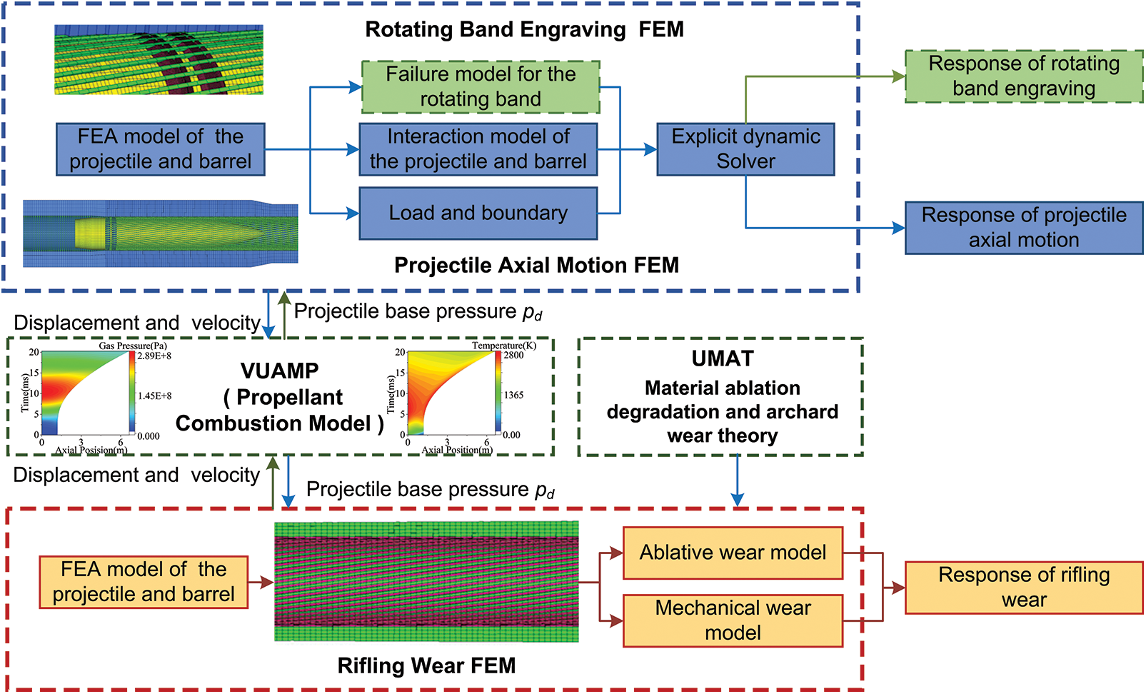
Figure 2: Comprehensive finite element model of artillery internal ballistics dynamics

The RAME models were integrated into the AIBD model in the form of the UMAT subroutine of ABAQUS, as shown in Fig. 2. This integration facilitates the computation of ablative wear within the inner bore and the assessment of mechanical wear on the rifling. Total rifling wear accumulates from both ablative and mechanical wear over successive shots. Through multiple shot simulations, we can obtain the total wear at each node of the rifling in the direction of the axis of the barrel, and thus the distribution of the rifling wear tired. The detailed calculation procedure can be found in the literature [17].

2.3 Model Simulation Results and Validation

The FEM results for the extrusion of an engraving band in different states are shown in Fig. 3a. The engraving resistance curve for the engraving process is shown in Fig. 3b. The results such as the maximum VonMises stress, the shape of the extrusion resistance curve, the maximum extrusion resistance, and the duration of the extrusion resistance at different moments of engraving demonstrated in these results are very close to the results of the Sun [43] experiment.

Figure 3: Simulation results of rotation band engraving

As shown in Fig. 4, the projectile axial motion model provides the time course curve of chamber pressure and the time course curve of the projectile’s axial velocity. The time-course curves from the projectile axial motion model are consistent with the studies of Yu et al. [41].

Figure 4: Projectile axial motion simulation and experimental results

The RAME model used in this paper was developed by Wang et al. [16,17]. The results of the RAME model are presented in Fig. 5. The figure shows the cumulative wear of the rifling after every 100 shots, in which the wear is mainly concentrated in the slope chamber, the beginning of the rifling, and the muzzle position. The cumulative ablative wear mainly occurs in the sloped chamber and the rifling initiation section, while the cumulative mechanical wear is mainly concentrated in the muzzle position. With the increase in the number of shots, the wear amount gradually increased. After the barrel has fired 500 rounds, the basic contour of the rifling is so worn that it can no longer reliably guide the projectile, resulting in the scrapping of the barrel.

Figure 5: The results of the rifling ablation and mechanical wear model

2.4 Systematic Decomposition of AIBD

2.4.1 Model Decomposition

Multiple FEMs, include the RBE model, the PAM model, and the RAME model, are utilized to depict the entire process of AIBD in this study. Since these models primarily concentrate on their inputs and outputs, they are considered “black-box” models and are referred to as subsystem analyzers in this paper. The output response fij from these subsystem analyzers is employed for optimizing performance indicators and designing constraints.

The goal of this paper is to address the challenge of achieving consistency between design variables in these “black boxes” or subsystems through the MDO method, an effective optimization strategy. The multidisciplinary solution framework for AIBD is illustrated in Fig. 6. This framework comprises four hierarchical levels: system-level, subsystem-level, surrogate models, and individual subsystem analyzers, presented in descending order.

Figure 6: The multidisciplinary solution framework for the AIBD problem

2.4.2 Experimental Design and Surrogate Modeling

Given that obtaining response fij from subsystems for this FEM is computationally intensive and impractical for direct online optimization, we employ design of experiments (DOE) and surrogate modeling to efficiently construct a relationship between the inputs and outputs of the subsystems. In MDO models, both system-level and subsystem optimizers utilize the approximate response f~ij to develop objective functions and constraints.

Due to the complexity of the AIBD finite element model used in this paper, each computation is time-consuming. Hence, it is essential to employ an effective Design of Experiments (DOE) method to reduce the number of sample points while ensuring a uniform distribution of samples in the design space. We have chosen the Optimal Latin Hypercube Design (OLHD) method, which further enhances the uniformity of the Latin Hypercube Design (LHD) through additional criteria. The OLHD approach ensures that the experimental sample matrix exhibits good projection uniformity across factor intervals and spatial uniformity within the sample space. Consequently, it allows the surrogate model to more accurately fit the relationship between the design variable space and response values.

In this study, a backpropagation (BP) surrogate model for each subsystem is developed utilizing the OLHD scheme and the BP surrogate model approach. The accuracy and generalization ability of these surrogate models are statistically validated using the coefficient of determination, R2, defined as follows:

R2=∑i=1n(yi−y^i)2∑i=1n(yi−y¯i)2(1)

where n represents the number of test samples; yi is the actual response of the finite element model for each test sample, with y¯i being the average of these actual responses; and y^i is the surrogate model response for each test sample. The R2 value closer to 1 indicates a higher similarity between the surrogate and finite element models. Table 1 lists the accuracy of these models for various response metrics in AIBD. With all models showing R2 values exceeding 0.92, this demonstrates a high level of reliability in the model’s accuracy.

3  A Novel Multi-Stage Multidisciplinary Design Optimization (MS-MDO) Method

This chapter proposes a multi-stage multidisciplinary design optimization (MS-MDO) approach based on collaborative optimization (CO) [24,39] algorithms. The essence of the approach is to decouple the coupled problem of coordinating design variables and comprehensive performance enhancement into two successive optimization stages: Stage I (MDO Stage) and Stage II, performance optimization (PO Stage). In the MDO Stage, a modified CO methodology is used to solve the complex system-level problem and accelerate the coordination of the shared design variables of the subsystems. Subsequently, in the PO Stage, to solve the problem that the subsystem performance metrics are not fully optimized. Specifically, in the MDO Stage, design variables are transferred to the system and subsystem after each system-level iteration as a new starting point to facilitate system-level convergence. In the PO Stage, the shared variables resulting from the MDO Stage are regarded as fixed parameters, while the local variables within each subsystem are designated as new design variables for enhancing the performance metrics of the subsystems to facilitate global optimization. The consecutive application of different optimization algorithms in two stages of the MS-MDO methodology effectively solves the comprehensive performance optimization challenges in complex engineering problems.

3.1 Stage I (MDO Stages) with CO Methods

The CO method is a two-layer optimization structure, which decomposes the problem into two levels: system and subsystem, and is suitable for solving multidisciplinary and highly complex engineering optimization problems. This system decomposition makes it possible to deal with global objectives at the system and local objectives at the subsystem at the same time. CO method can coordinate the design variables among subsystems efficiently by setting consistency constraints in order to achieve coordinated optimization of the system and the subsystem.

At the system-level optimization level, the primary objective is to optimize the overall system function fs while adhering to the consistency constraints Js∗ and system-level constraints gs. The consistency constraints Js∗ represent the differences between the system level and the subsystems. The design variables at the system level comprise the system design variable z and the coupled state variable between disciplines ys. The system design variable z is derived from the design variables shared by the disciplines. It is mathematically modeled as follows:

Find[z,ys]minfs(z,ys)s.t.Js∗=∑i=1n(‖z−x^i‖22+‖ys−y^i‖22)≤sgs(z,ys)≤0(2)

where s is the dynamic relaxation factor; x^i is the parameter passed to the system level by the ith subsystem, y^i is the parameter of the coupling state passed to the system level by the ith subsystem, and n is the number of subsystems.

At the level of subsystem optimization, the optimization objective is to minimize the consistency constraint Ji of the discipline while satisfying the constraint gi of the subsystem; since the design variables xi and coupled variables yi of the subsystems are related to the system-level transfer of the shared design variables z^s and coupled variables y^s spacing are minimized, respectively, and the optimization of the subsystems helps to advance the optimization of the whole system, which is mathematically modeled as:

Find[xi,xLi]minJi=∑i=1n(‖z^s−xi‖22+‖y^s−yi‖22)s.t.gi(xi,xLi)≤0yi=yi(xi,xLi,yj,j≠i)(3)

For the ith subsystem, the design variables consist of two parts: the shared design variable xi and the local design variable of the subsystem xLi, z^s and y^s represent the shared design variable and coupled variables passed to the subsystems at the system level, and the coupling variables yi are expected and remain constant during the optimization of the subsystem; yi are the coupling variable of the ith subsystem and calculated by the coupled variable analyzer yi=yi(xi,xLi,yj,j≠i); if neither the system level nor the subsystem involves coupled variables, then the parts related to the coupled variables yi in Eqs. (2) and (3) are omitted.

To solve the system-level convergence problem, this paper adopts the dynamic relaxation (DR) method, and the dynamic factor s in Eq. (2) is defined by the equation:

s=λ2ε2(4)

where λ is a control factor that satisfies 0.5 < λ < 1.0, ensuring that system-level optimization aims to reduce inter-disciplinary inconsistency; ε is the inter-disciplinary inconsistency information, which is calculated using the formula:

ε=∑j=1m‖x1j∗−x2j∗‖22(5)

where xij∗ is the jth design variable of the ith discipline after optimization and m is the total number of shared design variables.

3.2 Stage II (Performance Optimization Stage)

In the performance optimization stage, the optimization objective is to use the performance metrics obtained by the subsystem analyzer as the objective function of the individual subsystems, respectively, and its mathematical model is shown in Eq. (6):

Find[xLi]minJi=yi(xLi)s.t.gi(xLi)≤0yi=yi(z^s,xLi,yj,j≠i)(6)

For the ith subsystem, only the local design variables of the subsystem xLi are optimized as design variables, and the shared design variables z^s and the coupling variables yj and ys are used as fixed parameters substituted into the model using the optimized values from Stage I.

3.3 Procedure of MS-MDO Method

The implementation flowchart for the developed MS-MDO method is illustrated in Fig. 7. The computational steps are outlined as follows:

Figure 7: The MS-MDO method flowchart

Step 1: Define the optimization design problem, including the objective function, design variables, and constraint functions.

Step 2: Proceed to Stage I, the MDO Stage, and construct the MDO optimization model for the system and subsystems optimization problem.

Step 3: Initialize or update the design variables, starting points, boundaries, and other parameters at both the system and subsystem levels. And sequentially solve each subsystem to determine the design variables for each.

Step 4: Calculate the inconsistency information ε and the dynamic relaxation factor s among the systems. Solve the system-level optimization problem to obtain the shared design variables z.

Step 5: Check whether the system level meets the convergence consistency tolerance and the maximum iteration limit. If these criteria are satisfied, the iteration stops, and proceeds to output the optimal shared design variables at the system level and the performance indexes for each subsystem. If not, decide whether to apply the modified collaborative optimization method (M-DRCO) or the original collaborative optimization method (DRCO). For M-DRCO, return to Step 3, updating both system and subsystem level starting points to the shared design variables from the previous cycle, this is a significant advancement in the acceleration of system-level convergence within the MDO framework in this paper. For DRCO, also return to Step 3 but continue optimizing with the original starting points.

Step 6: Proceed to Stage II, the performance optimization stage. Construct the performance optimization model, treating the optimal shared design variables as fixed parameters. Redefine the objective function and design variables for each subsystem. Use the performance index of each subsystem as the new objective function and assign the subsystem’s local design variables as the design variables.

Step 7: Optimizing the solution for each subsystem in turn, output all optimal performance indices and design variables for both Stage I and Stage II.

4  Application Artillery Internal Ballistics Dynamics Based on MS-MDO Method

4.1 Definition of the AIBD Problem

4.1.1 Determination of Performance Metrics for AIBD

In evaluating the performance of artillery firing dynamics, it is crucial to consider several key aspects: safety of the bore firing process, muzzle kinetic energy, firing accuracy, and service life. For safety, the focus is on minimizing the engaging resistance of the rotation band. Projectile velocity at the muzzle is used to assess muzzle kinetic energy, with higher velocities being preferable [8]. Firing accuracy hinges on the projectile’s attitude at the muzzle [44], encompassing both the projectile’s lateral and vertical angular displacements at the muzzle, Ωym and Ωzm, as well as its lateral and vertical angular velocities, Φym and Φzm; lower values in these indicators signify higher accuracy. Lastly, rifling wear, which significantly affects the artillery’s service life [45], is evaluated with a focus on minimizing the maximum ablation wear (WSS) and mechanical wear (WJX) at each point along the rifling.

For the performance assessment of AIBD, four metrics are introduced to comprehensively reflect the firing performance. These metrics are the normalized engraving resistance coefficient ηfR, initial muzzle velocity coefficient ηvm, projectile disturbance coefficient at the muzzle ηds, and service life coefficient ηls. This constitutes a multi-objective optimization (MOO) problem. There are many methods to convert a multi-objective problem into a single objective optimization, such as decomposition-based methods [46,47], Pareto curve [48], and the linear weighting method [49] mentioned in this paper. In order to solve this MOO problem, in this paper, the weights of the objective function are calculated using the analytic hierarchy process (AHP) [50] method and the linear weighting method is used to convert this MOO problem into a single objective optimization design problem. The global objective function, F0, is then derived by summing these weighted objective functions. Moreover, to ensure generality and comparability, the performance metrics have been normalized, with normalization coefficients ϕi calculated based on their range of variation. Finally, Eq. (7) was employed to calculate the global objective F0.

F0=λ1ηfR+λ2ηvm+λ3ηds+λ4ηls=λ1fRϕfR+λ2ϕvxmvxm+λ3(abs(Ωym)ϕΩym+abs(Ωzm)ϕΩzm+abs(Φym)ϕΦym+abs(Φzm)ϕΦzm)+λ4(WSSϕWSS+WJXϕWJX)(7)

where ϕ∗ is the normalization factor, which is determined according to the range of variation of the response metrics, and the normalization factors are set as follows: ϕfr = 135, ϕvxm = 982, ϕΩym=1.6×10−3, ϕΩzm=0.6×10−3, ϕΦym = 1.97, ϕΦzm = 2.23; ϕWSS = 1.3, ϕWJX = 0.4, abs(∗) denotes the absolute value function; λi(i=1,2,3,4) is the weight coefficient, weight coefficients λ1=0.2, λ2=0.4, λ3=0.075, λ4=0.1, which are calculated using the AHP.

4.1.2 Definition of Constraint Function

In the context of optimizing AIBD, the prudent selection of constraint functions is paramount. This study delineates a comprehensive suite of constraint functions, meticulously considering a spectrum of factors that encompass safety, power, accuracy, and the extended longevity of the firing mechanism.

(1) Constraints of safety

Three constraints are considered for safety: 1) Engraving resistance (fR), set between 900~1600 kN [18,42], to ensure projectile stability during the engraving stage. 2) Projectile base pressure during engraving (Pd), where excessive pressure (165 MPa [7]) can lead to safety hazards like barrel explosions. 3) Maximum chamber pressure (Pm), crucial for firing performance, which could not exceed a specified limit (360 MPa [13]) to avoid structural damage to the gun. These corresponding constraint functions are articulated as follows:

gfR=|fR(b,tsh,W,ω,mp,α,e1,dRB)−1250|−350≤0(8)

gpd=Pd(b,tsh,W,ω,mp,α,e1,dRB)−165≤0(9)

gpm=pm(lc,b,tsh,W,ω,e1,lbd,lRB,lp,dp,W0)−360≤0(10)

(2) Constraints on the minimum muzzle velocity of the gun.

Minimum muzzle velocity, essential for firing performance, must exceed 950 m/s [13] to ensure adequate firing power.

gvxm=950−vxm(lc,b,tsh,W,ω,e1,lbd,lRB,lp,dp,W0)≤0(11)

(3) Constraints on artillery disturbance

The gun disturbance is effectively constraining it can minimize errors during the firing process and enhance accuracy. Consequently, limiting gun disturbance is considered a significant constraint in our study [13,51,52]. The constraints on the projectile’s lateral (Ωym) and vertical (Ωzm) angular displacement at the muzzle are outlined as:

gΩym=Ωym(lc,b,tsh,W,ω,e1,lbd,lRB,lp,dp,W0)−5.0×10−3≤0(12)

gΩzm=Ωzm(lc,b,tsh,W,ω,e1,lbd,lRB,lp,dp,W0)−2.0×10−3≤0(13)

The constraints on the projectile’s lateral (Φym) and vertical (Φzm) angular velocity at the muzzle are defined as:

gΦym=Φym(lc,b,tsh,W,ω,e1,lbd,lRB,lp,dp,W0)−6.4≤0(14)

gΦzm=Φzm(lc,b,tsh,W,ω,e1,lbd,lRB,lp,dp,W0)−1.9≤0(15)

(4) Constraints on the life of artillery firing

Rifling wear has been shown to lead to a reduction in muzzle velocity, generally not exceeding 10% over the lifespan of a gun, and is primarily associated with the number of shots fired, as evidenced by studies of Li et al. [45,53,54]. This study establishes the gun’s firing life at 500 rounds to balance power and accuracy, with mechanical wear capped at less than 0.58 mm and ablative wear at less than 2.2 mm [16,17]. Constraints of maximum ablative wear WSS and maximum mechanical wear WJX as follows:

gWSS=WSS(lc,b,tsh,W,ω,mp,α)−2.2≤0(16)

gWJX=WJX(lc,b,tsh,W,ω,mp,α)−0.58≤0(17)

4.1.3 Selection of the Design Variables

Scholars have delved into the sensitivity of various response indicators and their corresponding design variables of AIBD [7,14,55,56]. Drawing from their insights, we have selected [btshWωmpαe1dRB] as the design variables for the RBE subsystem, where b is the groove width, tsh is the rifling depth, W is the rotating band width, ω is the powder mass, mp is the projectile mass, α is the forcing cone angle, e1 is the powder thickness, dRB is the outer diameter of the rotating band. For the PAM subsystem, the design variable is [lcbtshWωe1lbdlRBlpdpW0], where lc is the mass eccentricity of the projectile, lbd is the bourrelet-to-rifling distance, lRB is the rotating band location, lp is the powder length, dp is the powder aperture, W0 is the propellant chamber. Additionally, [lcbtshWωmpα] are identified as the design variables for the RAME subsystem.

4.2 Mathematical Model of Stage I (MDO Stages) for AIBD

Next, we detail the system-level optimization model and the subsystem-level models within the relaxation-variable-based collaborative optimization framework for artillery firing dynamics.

4.2.1 Optimization Model of the System-Level

The system-level optimization model can be represented by Eq. (18) as:

Findz=[lcbtshWωmpαe1]minzFs=F0+Jsysa+Jsysb+Jsyscs.t.Jsysa=(b−b^a)2+(tsh−t^sha)2+(W−W^a)2+(ω−ω^a)2+(mp−m^pa)2+(α−α^a)2+(e1−e^1a)2−s≤0Jsysb=(lc−l^cb)2+(b−b^b)2+(tsh−t^shb)2+(W−W^b)2+(ω−ω^b)2+(α−α^b)2+(e1−e^1b)2−s≤0Jsysc=(lc−l^cc)2+(b−b^c)2+(tsh−t^shc)2+(W−W^c)2+(ω−ω^c)2+(mp−m^pc)2+(α−α^c)2+(e1−e^1c)2−s≤0(18)

where z is the shared design variable; Jsysa, Jsysb, Jsysc are the consistency constraint function for subsystem a, subsystem b, and subsystem c, respectively, where ∗^a, ∗^b and ∗^c are copies of the parameters from subsystems a, subsystem b, and subsystem c, and s are the relaxation factors; F0 a is the global objective function of Eq.(7).

4.2.2 Optimization Model of the RBE Subsystem

The optimization model for the rotation band engraving subsystem is presented as Eq. (19):

Findx=[xaxLa]=[btshWωmpαe1dRB]minxJsys a=(b−b^)2+(tsh−t^sh)2+(W−W^)2+(ω−ω^)2+(mp−m^p)2   +(α−α^)2+(e1−e^1)2s.t.gfR≤0,gpd≤0(19)

where the design variable x consists of the shared design variable xa and the local design variable xLa=[dRB]; Jsysa is the consistency constraint function and Jsysa also is the optimization objective of the RBE subsystem; gfR and gpd are the constraint function of Eqs. (8) and (9).

4.2.3 Optimization Model of the PAM Subsystem

The optimization model for the projectile’s axial motion subsystem is presented in Eq. (20):

Findx=[xbxLb]=[lcbtshWωe1lbdlRBlpdpW0]minxJsubb=(lc−l^c)2+(b−b^)2+(tsh−t^sh)2+(W−W^)2+(ω−ω^)2+(e1−e^1)2s.t.gpm≤0,gvxm≤0,gΩym≤0,gΩzm≤0,gΦym≤0,gΦzm≤0(20)

where the design variable x consists of the shared design variable xb and the local design variable xLb=[lbdlRBlpdpW0]; Jsubb is the consistency constraint function, and is the optimization objective of the PAM subsystem; gpm, gvxm, gΩym, gΩzm, gΦym and gΦzm are constraint functions from the Eqs. (10) ~ (15).

4.2.4 Optimization Model of RAME Subsystem

The optimization model for the rifling wear subsystem is presented in Eq. (21):

Find x=[xc]=[lcbtshWωmpα]minx Jsubc=(lc−l^c)2+(b−b^)2+(tsh−t^sh)2+(W−W^)2+(ω−ω^)2   + (mp−m^p)2+(α−α^)2s.t. gWSS≤0,gWJX≤0(21)

where the design variables x are all composed of shared design variables xc, and there are no local design variables; Jsubc is the consistency constraint function, and is the optimization objective of the RAME subsystem; gWSS and gWJX are the constraint functions from the Eqs. (16) and (17).

4.3 Mathematical Model of Stage II (PO Stage) for AIBD

Both the RBE and PAM subsystems include local design variables in their respective optimization models as listed in Eqs. (20) and (21). Therefore, optimizing these local variables within the subsystems is essential for improving the overall performance index.

4.3.1 Optimization Model for the Performance of the Rotating Band Subsystem

The optimization model for the rotating band subsystem is delineated in Eq. (22) as follows:

Findx=[xLa]=[dRB]minxf=fR(dRB)s.t.gfR≤0,gpd≤0(22)

where the design variable x is the local design variable dRB, the objective function is the engraving resistance fR. It is worth noting that when using a surrogate model to solve for the performance metrics at the PO stage, the optimal values z∗=[lcbtshWωmpαe1] obtained at the MDO stage, need to be substituted as parameters into the model.

4.3.2 Optimization Model for the Performance of Projectile Movement in the Barrel Subsystem

The performance optimization model for projectile movement within the barrel subsystem is presented in Eq. (23):

Findx=[xLb]=[lbdlRBlpdpW0]minxf=λ2ϕvxmvxm+λ3(abs(Ωym)ϕΩym+abs(Ωzm)ϕΩzm+abs(Φym)ϕΦym+abs(Φzm)ϕΦzm)s.t.gpm≤0,gvxm≤0,gΩym≤0,gΩzm≤0,gΦym≤0,gΦzm≤0(23)

where the design variable x consists of the local design variable xLb = [lbdlRBlpdpW0], the objective function is a multi-objective function consisting of the normalized muzzle velocity and normalized with the projectile perturbation coefficient, and the weight coefficients λ2=0.4, λ3=0.075 are same as the weight coefficients of MDO stage in the system-level objective function, as in Eq. (7).

4.4 Optimization Process and Results

The boundary of design variables settings for both system-level and subsystem are detailed in Tables 2 and 3. Considering the influence of the initial values of the system-level shared design variables on the convergence results, in order to objectively evaluate the research methodology, we set four sets of initial values for these variables, which are listed in rows 3 to 6 of Table 2.

Sequential Least Squares Optimization (SLSQP) is a local optimization algorithm based on gradient information that solves nonlinear minimization problems with constraints. Scipy.SLSQP has been utilized as the optimizer at both the system and subsystem levels during the MDO Stage to solve complex constraints in order to ensure the convergence stability of the CO method. The results of the system-level calculations using both the original and modified CO methods Stage I are presented in Table 4.

The RBE and PAM subsystems have been transformed into single-objective optimization problems in the PO Stage, unlike the two-level nested optimization challenges in the MDO Stage. Pygmo2.GPPSO (Gaussian Process and Particle Swarm Optimization) [57] is an intelligent optimization algorithm that performs well in global optimization search. Pygmo2. GPPSO optimizer was used as the optimizer in Stage II, the population size of GPPSO was set to 200 and the number of iteration generations was set to 1000, the performance of Stages I and II based on the M-DRCO strategy are presented in Table 5.

From Table 4, the CO and M-CO strategies are convergent at all starting points, i.e., they all satisfy the consistency convergence condition (Jsysi < 1 × 10−4). By comparing the number of iterations and evaluations for the original CO and M-CO, it is clear that the M-CO strategy significantly outperforms the original.

Taking the starting point 4 as an example, Fig. 8 shows the convergence iteration of the M-DRCO algorithm. Fig. 8b shows ε1, ε2, and ε3 calculated according to Eq. (6), which represents the three inter-disciplinary inconsistency information described in this paper (i.e., RBE model, PAM model, and RAME model). The system level is considered to have a feasible solution only when all three inconsistency information values are simultaneously less than or equal to the dynamic scaling factor s. As shown in Fig. 8a, at the starting point 4, only three iterations produced a feasible solution, even though there were 19 iterations at the system level.

Figure 8: The convergence curves of MS-MDO strategy at the starting point 4 (Uniformly denoted by 1E-10 when E < 1E-10 or less in Fig. 8b)

Consider that the number of times the algorithm evaluates the objective function (or loss function) is the number of evaluations, especially when “black-box” models are involved (e.g., hydrodynamics or explicit dynamics finite element models), where each evaluation incurs a high computational cost. Consequently, the M-DRCO strategy aimed at reducing the number of evaluations can significantly lower the overall computational costs. As can be seen from the data in column 4 of Table 4, the M-DRCO algorithm has fewer iterations compared to the DRCO algorithm under all different starting points. Fig. 8 demonstrates the effectiveness of the M-DRCO strategy with the convergence curves of the objective function, the consistency constraint function, and the relaxation factors at the starting point 4. The M-DRCO strategy adopts the dynamic relaxation (DR) factor s to dynamically adjust the consistency constraints, thus accelerating the convergence speed, and the system-level convergence is realized in only 19 iterations. This reveals that the M-DRCO strategy effectively improves the convergence speed by reducing the number of evaluations of the “black-box” model, which in turn effectively reduces the computational cost.

Statistical analysis of the data in Table 5 reveals changes in performance indices as depicted in Fig. 9. Implementing the M-DRCO strategy leads to a significant reduction of 18.7% in average engraving resistance in Stage II compared to Stage I, with values engraving resistance near the 900 kN constraint. While the increase in projectile velocity at the muzzle is modest at 1.15%, it still represents an improvement over Stage I, exemplified by reaching 1005 m/s at starting point 1. Moreover, the normalized projectile disturbance coefficient dramatically decreases by 59.8%. These findings underscore the M-DRCO strategy’s substantial optimization effect in Stage II.

Figure 9: Change rate of each performance index

An in-depth analysis of Eqs. (18) to (21) within the CO strategy uncovers the reasons behind the effectiveness of the MS-MDO approach, as proposed in this paper, for addressing engineering optimization problems that involve local design variables in subsystems. Since the core function of the CO strategy at the system level is primarily to coordinate shared design variables, excluding the local design variables of subsystems; the subsystem objective function is limited to consistency constraints and does not include performance metrics. When after satisfying the local constraints, the local design variables do not contribute to optimizing performance indices. Therefore, the CO strategy is limited to addressing the coordination problem of design variables and coupling variables among subsystems, without further enhancing the performance index. In Stage II, we further optimized the local design variables through the application of performance optimization methods. This approach significantly improves the performance metrics and proves the effectiveness of this stage in enhancing the performance of the system.

In summary, the MS-MDO method proposed in this paper effectively reduces the number of iterations and evaluations while successfully coordinating the optimization of the design variables in Stage I, and improves the performance metrics in Stage II, which achieves the original intention of this paper.

4.5 Validation of Optimization Results for AIBD

It can be found in Table 5 that starting point 4 has a better overall performance after the M-DRCO strategy optimized in Stage I and Stage II. The optimized system shared design variables and the local design variables of each subsystem are recombined into the design parameters of each subsystem and substituted into the FEMs of RBE, PAM, and RAME described in Section 2.2 sequentially for simulation to obtain the computational results, as Figs. 10 to 12.

Figure 10: Compare the engraving resistances and velocities for Stage I and Stage II

Figure 11: Compare the projectile attitude change along the barrel for Stage I and Stage II

Figure 12: Variation of rifling wear along the barrel after accumulating 500 shots

Fig. 10a demonstrates the engraved resistance comparison between Stages I and II, derived from the RBE finite element model using optimized parameters from both stages. Figs. 10b and 11 present the projectile’s velocity, chamber pressure, and attitude during axial movement calculated with the PAM finite element model and its optimized parameters. Additionally, Fig. 12 illustrates the rifling wear variation along the barrel’s axial direction after 500 shots, as simulated with the RAME finite element model using optimized parameters.

These validation curves affirm that the finite element model’s outcomes align with the surrogate model’s performance obtained through the MS-MDO method, verifying the surrogate model’s effectiveness. Notably, performance enhancements in Stage II, such as reduced engraving resistance and increased muzzle velocity, significantly surpass those in Stage I. This underscores that the MS-MDO method successfully enhances the overall performance of artillery internal ballistics by effectively coordinating parameters across various subsystem models.

5  Conclusion

This study introduces a multi-stage multidisciplinary optimization (MS-MDO) method to address the challenge of enhancing the comprehensive performance of the comprehensive artillery internal ballistic dynamics (AIBD) model. The power, accuracy, and lifetime of artillery firing are improved through the MS-MDO method. These research results provide effective methods and strategies for artillery design and performance enhancement and are expected to have a positive impact on the military field and engineering practice.

1) This study established and validated a comprehensive ballistic dynamics model in artillery, integrating the propellant combustion model, the rotation band engraving model, the projectile axial motion, and the rifling wear model. The model was effectively decomposed into subsystems using a system engineering approach. We then applied a multi-stage multidisciplinary optimization (MS-MDO) method to address the optimization challenges of both the reducer model and the AIBD model, demonstrating the method’s efficacy through validation.

2) The Stage I (MDO Stage), featuring the M-DRCO method proposed in this paper, showcased considerable benefits. It significantly reduced the number of iterations and evaluations, thereby cutting computational costs. The method enhanced the convergence speed of the consistency constraint function and effectively coordinated shared variables across different stages’ optimization models.

3) In Stage II (Performance Optimization), we observed substantial improvements in performance metrics over Stage 1 results. Notably, the average engraving resistance was reduced by 18.7% in Stage 2. The normalized projectile disturbance coefficient decreased by 59.8%, and while the increase in muzzle velocity was modest, it achieved satisfactory levels.

The MS-MDO method proposed in this paper has achieved remarkable results and can be further generalized for use in complex engineering problems. Furthermore, its effectiveness is mainly limited to subsystems containing local design variables, and the traditional CO method may be more suitable for systems that do not contain local design variables. In addition, the sensitivity of this study’s method to the starting design point may limit its ability to directly obtain a globally optimal solution in some cases.

Looking ahead, integrating uncertainty factors with multidisciplinary design optimization (MDO) and exploring the combination of multi-objective optimization with MDO is pivotal for enhancing optimization stability and tackling complex engineering challenges.

Acknowledgement: The authors express their appreciation to Bing Wang, Fengjie Xu, and Shuli Li of Nanjing University of Science and Technology for developing a finite element mesh model of the artillery internal ballistics dynamic models based on the parameters specified in the experimental design table. And thanks to Yu Fang from Nanjing University of Science and Technology Zijin College for debugging the code. Besides, the authors wish to express their many thanks to the reviewers for their useful and constructive comments.

Funding Statement: This research was financially supported by the “National Natural Science Foundation of China” (Grant Nos. 52105106, 52305155), the “Jiangsu Province Natural Science Foundation” (Grant Nos. BK20210342, BK20230904), the “Young Elite Scientists Sponsorship Program by CAST” (Grant No. 2023JCJQQT061).

Author Contributions: The authors confirm contribution to the paper as follows: study conception and design: Jipeng Xie, Guolai Yang; data collection: Liqun Wang; analysis and interpretation of results: Jipeng Xie, Lei Li; draft manuscript preparation: Jipeng Xie. All authors reviewed the results and approved the final version of the manuscript.

Availability of Data and Materials: Due to the ongoing nature of the project on which this research is based, the original data cannot be publicly shared. For those interested in this study, please contact the corresponding author of this paper for further information and access to the relevant data.

Conflicts of Interest: The authors declare that they have no conflicts of interest to report regarding the present study.

References

1. Gonzalez, J. R. (1990). Interior ballistics optimization (Ph.D. Thesis). Kansas State University, Manhattan, USA. [Google Scholar]

2. Li, K., Zhang, X. (2011). Multi-objective optimization of interior ballistic performance using NSGA-II. Propellants, Explosives, Pyrotechnics, 36(3), 282–290. https://doi.org/10.1002/prep.201000027 [Google Scholar] [CrossRef]

3. Cheng, C., Zhang, X. (2012). Interior ballistic charge design based on a modified particle swarm optimizer. Structural and Multidisciplinary Optimization, 46(2), 303–310. https://doi.org/10.1007/s00158-012-0768-6 [Google Scholar] [CrossRef]

4. Xin, T., Yang, G., Wang, L., Sun, Q. (2020). Numerical calculation and uncertain optimization of energy conversion in interior ballistics stage. Energies, 13(21), 5824. https://doi.org/10.3390/en13215824 [Google Scholar] [CrossRef]

5. Wang, M., Jin, G., Zhou, Y., Nan, F., Lin, X. et al. (2022). Integration of complex geometry gun propellant form function calculation and geometry optimization. Propellants, Explosives, Pyrotechnics, 47(9), e202200062. https://doi.org/10.1002/prep.202200062 [Google Scholar] [CrossRef]

6. Wang, J., Yu, Y., Zhou, L., Ye, R. (2018). Numerical simulation and optimized design of cased telescoped ammunition interior ballistic. Defence Technology, 14(2), 119–125. https://doi.org/10.1016/j.dt.2017.11.006 [Google Scholar] [CrossRef]

7. Hu, C., Zhang, X. (2019). Influence of multiple structural parameters on interior ballistics based on orthogonal test methods. Defence Technology, 15(5), 690–697. https://doi.org/10.1016/j.dt.2019.06.014 [Google Scholar] [CrossRef]

8. Wang, L., Chen, Z., Yang, G. (2021). An uncertainty analysis method for artillery dynamics with hybrid stochastic and interval parameters. Computer Modeling in Engineering & Sciences, 126(2), 479–503. https://doi.org/10.32604/cmes.2021.011954 [Google Scholar] [CrossRef]

9. Cao, R., Zhang, X. (2019). Design optimization for a launching system with novel structure. Defence Technology, 15(5), 680–689. https://doi.org/10.1016/j.dt.2019.08.005 [Google Scholar] [CrossRef]

10. Cao, R., Zhang, X. (2019). A novel launching system applying a relay chamber technology and its optimization. Propellants, Explosives, Pyrotechnics, 44(9), 1199–1205. https://doi.org/10.1002/prep.201800242 [Google Scholar] [CrossRef]

11. Chaturvedi, E. (2020). Numerical investigation of dynamic interaction with projectile and harmonic behaviour for T-finned machine gun barrels. Defence Technology, 16(2), 460–469. https://doi.org/10.1016/j.dt.2019.07.018 [Google Scholar] [CrossRef]

12. Xiao, H., Yang, G., Ge, J. (2017). Surrogate-based multi-objective optimization of firing accuracy and firing stability for a towed artillery. Journal of Vibroengineering, 19(1), 290–301. https://doi.org/10.21595/jve.2016.17108 [Google Scholar] [CrossRef]

13. Xu, F., Yang, G., Wang, L. (2021). Artillery structural dynamic responses uncertain optimization based on robust Nash game method. Journal of Mechanical Science and Technology, 35(9), 4093–4104. https://doi.org/10.1007/s12206-021-0821-8 [Google Scholar] [CrossRef]

14. Ding, C., Liu, N., Zhang, X. (2017). A mesh generation method for worn gun barrel and its application in projectile-barrel interaction analysis. Finite Elements in Analysis and Design, 124, 22–32. https://doi.org/10.1016/j.finel.2016.10.003 [Google Scholar] [CrossRef]

15. Shen, C., Zhou, K., Lu, Y., Li, J. (2019). Modeling and simulation of bullet-barrel interaction process for the damaged gun barrel. Defence Technology, 15(6), 972–986. https://doi.org/10.1016/j.dt.2019.07.009 [Google Scholar] [CrossRef]

16. Li, S., Wang, L., Xu, F., Yang, G. (2023). Numerical simulations for artillery barrel temperature variation considering mechanical friction heat under continuous shots. International Communications in Heat and Mass Transfer, 142, 106663. https://doi.org/10.1016/j.icheatmasstransfer.2023.106663 [Google Scholar] [CrossRef]

17. Wang, L., Li, S., Xu, F., Yang, G. (2022). United computational model for predicting thermochemical-mechanical erosion in artillery barrel considering friction behavior. Case Studies in Thermal Engineering, 29, 101726. https://doi.org/10.1016/j.csite.2021.101726 [Google Scholar] [CrossRef]

18. Sun, Q., Yang, G., Ge, J. (2016). Modeling and simulation on engraving process of projectile rotating band under different charge cases. Journal of Vibration and Control, 23(6), 1044–1054. https://doi.org/10.1177/1077546315587806 [Google Scholar] [CrossRef]

19. Hui, J., Gao, M., Li, X. (2018). Dynamic response for shock loadings and stress analysis of a trajectory correcting fuse based on fuse-projectile–barrel coupling. The Journal of Defense Modeling and Simulation: Applications, Methodology, Technology, 15(3), 351–364. https://doi.org/10.1177/1548512918757693 [Google Scholar] [CrossRef]

20. Wei, Z., Wang, F. (2018). Overall parameters design and optimization system for gun and bullet. International Journal of Materials, Mechanics and Manufacturing, 6(1), 1–7. https://doi.org/10.18178/ijmmm.2018.6.1.337 [Google Scholar] [CrossRef]

21. Shen, Q., Yan, L., Zhao, J., Gao, Y., Yuan, Y. et al. (2023). Projectile artillery propellant coupled optimization design method of artillery weapon systems. Journal of Physics: Conference Series, 2460(1), 12047. https://doi.org/10.1088/1742-6596/2460/1/012047 [Google Scholar] [CrossRef]

22. Xie, J., Yang, G., Sun, Q. (2023). Modified enhanced collaborative optimization method for artillery launching dynamic model with sequential process. Journal of Low Frequency Noise, Vibration and Active Control, 42(2), 654–672. https://doi.org/10.1177/14613484221114883 [Google Scholar] [CrossRef]

23. Brown, N. F., Olds, J. R. (2006). Evaluation of multidisciplinary optimization techniques applied to a reusable launch vehicle. Journal of Spacecraft and Rockets, 43(6), 1289–1300. https://doi.org/10.2514/1.16577 [Google Scholar] [CrossRef]

24. Kroo, I., Altus, S., Braun, R., Gage, P., Sobieski, I. (1994). Multidisciplinary optimization methods for aircraft preliminary design. 5th Symposium on Multidisciplinary Analysis and Optimization, pp. 697–707. Florida, USA. https://doi.org/10.2514/6.1994-4325 [Google Scholar] [CrossRef]

25. Braun, R. D. (1996). Collaborative optimization: An architecture for large-scale distributed design (Ph.D Thesis). Stanford University, Stanford, USA. [Google Scholar]

26. Braun, R. D., Moore, A. A., Kroo, I. M. (1997). Collaborative approach to launch vehicle design. Journal of Spacecraft and Rockets, 34(4), 478–486. https://doi.org/10.2514/2.3237 [Google Scholar] [CrossRef]

27. Zhao, W., Yang, Z., Wang, C. (2018). Multidisciplinary hybrid hierarchical collaborative optimization of electric wheel vehicle chassis integrated system based on driver’s feel. Structural and Multidisciplinary Optimization, 57(3), 1129–1147. https://doi.org/10.1007/s00158-017-1801-6 [Google Scholar] [CrossRef]

28. Tao, S., Shintani, K., Yang, G., Meingast, H., Apley, D. W. et al. (2018). Enhanced collaborative optimization using alternating direction method of multipliers. Structural and Multidisciplinary Optimization, 58(4), 1571–1588. https://doi.org/10.1007/s00158-018-1980-9 [Google Scholar] [CrossRef]

29. Meng, D., Yang, S., Jesus, A. M. de, Zhu, S. (2023). A novel Kriging-model—assisted reliability—based multidisciplinary design optimization strategy and its application in the offshore wind turbine tower. Renewable Energy, 203, 407–420. https://doi.org/10.1016/j.renene.2022.12.062 [Google Scholar] [CrossRef]

30. Chu, C., Yin, C., Shi, S., Su, S., Chen, C. (2023). Multidisciplinary modeling and optimization method of remote sensing satellite parameters based on SysML-CEA. Computer Modeling in Engineering & Sciences, 135(2), 1413–1434. https://doi.org/10.32604/cmes.2022.022395 [Google Scholar] [CrossRef]

31. Meng, D., Yang, S., Lin, T., Wang, J., Yang, H. et al. (2022). RBMDO using Gaussian mixture model-based second-order mean-value saddlepoint approximation. Computer Modeling in Engineering & Sciences, 132(2), 553–568. https://doi.org/10.32604/cmes.2022.020756 [Google Scholar] [CrossRef]

32. Jin, X., Duan, F., Chen, P., Yang, Y. (2017). A robust global optimization approach to solving CO problems—enhanced design space decrease collaborative optimization. Structural and Multidisciplinary Optimization, 55(6), 2305–2322. https://doi.org/10.1007/s00158-016-1644-6 [Google Scholar] [CrossRef]

33. Fazeley, H. R., Taei, H., Naseh, H., Mirshams, M. (2016). A multi-objective, multidisciplinary design optimization methodology for the conceptual design of a spacecraft bi-propellant propulsion system. Structural and Multidisciplinary Optimization, 53(1), 145–160. https://doi.org/10.1007/s00158-015-1304-2 [Google Scholar] [CrossRef]

34. Huang, H., Tao, Y., Liu, Y. (2008). Multidisciplinary collaborative optimization using fuzzy satisfaction degree and fuzzy sufficiency degree model. Soft Computing, 12(10), 995–1005. https://doi.org/10.1007/s00500-007-0268-6 [Google Scholar] [CrossRef]

35. Li, H., Ma, M., Zhang, W. (2014). Improving collaborative optimization for MDO problems with multi-objective subsystems. Structural and Multidisciplinary Optimization, 49(4), 609–620. https://doi.org/10.1007/s00158-013-0995-5 [Google Scholar] [CrossRef]

36. Sobieski, I., Kroo, I. M. (2000). Collaborative optimization using response surface estimation. AIAA Journal, 38(10), 1931–1938. https://doi.org/10.2514/6.1998-915 [Google Scholar] [CrossRef]

37. Zadeh, P. M., Toropov, V. V., Wood, A. S. (2009). Metamodel-based collaborative optimization framework. Structural and Multidisciplinary Optimization, 38(2), 103–115. https://doi.org/10.1007/s00158-008-0286-8 [Google Scholar] [CrossRef]

38. Li, H., Jing, Y., Ma, M., Zhang, S. (2009). Collaborative optimization algorithm based on dynamic penalty function method. Control and Decision, 24(6), 911–915+920 (In Chinese). [Google Scholar]

39. Li, X., Li, W., Liu, C. (2008). Geometric analysis of collaborative optimization. Structural and Multidisciplinary Optimization, 35(4), 301–313. https://doi.org/10.1007/s00158-007-0127-1 [Google Scholar] [CrossRef]

40. Hu, C., Zhang, X. (2018). A fluid-structure coupling method to obtain parameter distributions in a combustion chamber with moving boundaries. Applied Thermal Engineering, 141, 1048–1054. https://doi.org/10.1016/j.applthermaleng.2018.06.063 [Google Scholar] [CrossRef]

41. Yu, Q., Yang, G. (2019). Dynamic stress analysis on barrel considering the radial effect of propellant gas flow. Journal of Pressure Vessel Technology, 141(1), 746. https://doi.org/10.1115/1.4041974 [Google Scholar] [CrossRef]

42. Li, Z., Ge, J., Yang, G., Tang, J. (2016). Modeling and dynamic simulation on engraving process of rotating band into rifled barrel using three different numerical methods. Journal of Vibroengineering, 18(2), 768–780. [Google Scholar]

43. Sun, Q. (2016). Study on dynamics of rotating band engraving for large caliber howitzers (Ph.D. Thesis). Nanjing University of Science and Technology, Nanjing, China (In Chinese). [Google Scholar]

44. Qian, L., Chen, G., Tong, M., Tang, J. (2022). General design principle of artillery for firing accuracy. Defence Technology, 18(12), 2125–2140. https://doi.org/10.1016/j.dt.2022.09.001 [Google Scholar] [CrossRef]

45. Li, X., Mu, L., Zang, Y., Qin, Q. (2020). Study on performance degradation and failure analysis of machine gun barrel. Defence Technology, 16(2), 362–373. https://doi.org/10.1016/j.dt.2019.05.008 [Google Scholar] [CrossRef]

46. Tomczyk, M. K., Kadzinski, M. (2020). Decomposition-based interactive evolutionary algorithm for multiple objective optimization. IEEE Transactions on Evolutionary Computation, 24(2), 320–334. https://doi.org/10.1109/TEVC.2019.2915767 [Google Scholar] [CrossRef]

47. Tomczyk, M. K., Kadziński, M. (2021). Decomposition-based co-evolutionary algorithm for interactive multiple objective optimization. Information Sciences, 549, 178–199. https://doi.org/10.1016/j.ins.2020.11.030 [Google Scholar] [CrossRef]

48. Lu, C., Huang, Y., Meng, L., Gao, L., Zhang, B. et al. (2022). A Pareto-based collaborative multi-objective optimization algorithm for energy-efficient scheduling of distributed permutation flow-shop with limited buffers. Robotics and Computer-Integrated Manufacturing, 74, 102277. https://doi.org/10.1016/j.rcim.2021.102277 [Google Scholar] [CrossRef]

49. Marler, R. T., Arora, J. S. (2010). The weighted sum method for multi-objective optimization: New insights. Structural and Multidisciplinary Optimization, 41(6), 853–862. https://doi.org/10.1007/s00158-009-0460-7 [Google Scholar] [CrossRef]

50. Saaty, T. L., Vargas, L. G. (2001). Models, methods, concepts & applications of the analytic hierarchy process. In: International series in operations research & management science, vol. 34. Boston, MA: Springer US. [Google Scholar]

51. Qian, L., Chen, G. (2017). The uncertainty propagation analysis of the projectile-barrel coupling problem. Defence Technology, 13(4), 229–233. https://doi.org/10.1016/j.dt.2017.06.005 [Google Scholar] [CrossRef]

52. Wang, M., Qian, L., Chen, G., Lin, T., Shi, J. et al. (2023). High-dimensional uncertainty quantification of projectile motion in the barrel of a truck-mounted howitzer based on probability density evolution method. Defence Technology. https://doi.org/10.1016/j.dt.2023.03.004 [Google Scholar] [CrossRef]

53. Jin, W., Feng, S., Xv, D. (2014). Extraplotation technology and engineering practice for gun barrel life in the approval test. Beijing, China: National Defence Industry Press. [Google Scholar]

54. Ma, J. (2018). The law of barrel wear and its application. Defence Technology, 14(6), 674–676. https://doi.org/10.1016/j.dt.2018.06.012 [Google Scholar] [CrossRef]

55. Liu, F., Song, Y., Yu, H., Lin, W., Zhang, J. et al. (2018). Study on the influence of projectile on muzzle disturbance. Defence Technology, 14(5), 570–577. https://doi.org/10.1016/j.dt.2018.07.016 [Google Scholar] [CrossRef]

56. Leonhardt, D., Garnich, M., Lucic, M. (2022). Analysis of the effect of bore centerline on projectile exit conditions in small arms. Defence Technology, 18(12), 2160–2169. https://doi.org/10.1016/j.dt.2021.09.008 [Google Scholar] [CrossRef]

57. Biscani, F., Izzo, D. (2020). A parallel global multiobjective framework for optimization: Pagmo. Journal of Open Source Software, 5(53), 2338. https://doi.org/10.21105/joss.02338 [Google Scholar] [CrossRef]