Uncertainty-Aware Physical Simulation of Neural Radiance Fields for Fluids

1  Introduction

With the exponential growth of computational power, deep learning [1] has achieved tremendous success across a wide variety of scientific disciplines [2–4]. Many studies have shown that deep learning techniques hold great promise for predicting complex phenomena associated with fluids [5]. In the area of computational mechanics, Physics-informed Neural Networks (PINNs) [6] has become an appealing alternative to classical numerical simulators for solving partial differential equations. Compared to conventional numerical algorithms like fluid volume methods [7] and finite element methods [8], PINNs cannot only be used as a surrogate model to accelerate forward computation but more importantly are suitable for inverse and optimization problems due to the ease of computation of gradients. On the other hand, due to encoding physical laws, PINNs are more robust than pure data-driven simulation to noisy and sparse data.

Three-dimensional (3D) reconstruction from two-dimensional (2D) RGB images or video frames is an important research topic in computational graphics, whose goal is to infer three-dimensional geometry and scenes from multiple 2D images. T. Neural radiance fields (NeRFs) have attracted enormous attention since it was introduced in 2020 [9]. NeRF achieved photo-realistic novel view synthesis using implicit representations in the supervision of 2D images. It is able to accurately describe complex optical phenomena such as lighting, shadowing, reflection, and refraction in the scene. It is also extended to simulate transparent and translucent objects, as well as intricate light propagation effects like scattering and absorption, which are difficult for traditional techniques [10] with discrete voxels or point clouds.

In computational fluid mechanics, reconstructing dynamic fluid fields with high fidelity from sparse multi-view RGB videos remains a formidable task due to the complexity of underlying physics. The pioneering work of Chu et al. [11] combines PINN with NeRF for smoke reconstruction, leveraging sparse video frames and physical laws to supervise the learning of continuous spatio-temporal radiance fields and velocity fields in dynamic scenes. Chu’s work [11] makes a significant contribution to fluid reconstruction by integrating the techniques in computational fluid mechanics, deep learning, and computer graphics. Compared to traditional methods, high-fidelity 3D models of dynamic fluids can be obtained with only end-to-end neural network training and supervision of 2D images.

Due to a lack of cognitive knowledge of unobserved regions of the scene, there is inherent uncertainty when synthesizing novel views from images. Quantifying such uncertainties is particularly important in fluid reconstruction because it influences not only the quality of imagery but also the accuracy of physics fields (e.g., fluid velocity). Hence, there is a pressing demand to develop a simple and scalable framework for uncertainty analysis. Some progress has been made in this direction for the NeRF model. For instance, Shen et al. [12,13] proposed Stochastic Neural Radiance Fields (S-NeRF) and Conditional Flow Neural Radiance Fields (CF-NeRF), both of which incorporate uncertainty quantification into NeRF-based methods to model the uncertainty associated with scene information. Inspired by the pioneering work, in this study, we leverage ensemble learning for uncertainty analysis of the smoke reconstruction process based on a combination of NeRF and PINN. By capturing the mean and standard deviation of the response of the fluid system, the reliability of the model and its sensitivity to anomalies can be understood. Moreover, the information on the uncertainties enhances the robustness of downstream tasks of 3D reconstruction, for example, reliability analysis, engineering design, and robotic visual perception.

The proposed work is based on Chu’s algorithm in smoke reconstruction [11] and introduces the uncertainty quantification module [14]. Our contribution can be summarized as follows:

•   By introducing ensemble learning, we conducted synchronized training on multiple NeRFs and PINNs. The average values of the results from multiple models was used as the final prediction, and the standard deviation in the predictions quantified the model’s uncertainty.

•   We extended the PINN based on a fully connected neural network by adding residual blocks and a two-layer activation function (sinusoidal space), which greatly improves the robustness and efficiency of the algorithm.

•   Conventional NeRF structure often suffers from overfitting problems. To address this issue, we employ frequency regularization of FreeNeRF [15] to prevent high-frequency information from converging too fast by constraining positional coding information.

2  Related Work

2.1 Implicit Neural Representations and NeRF

In computational graphics, signals are often represented discretely and explicitly. For example, images are represented as discrete grids of pixels, and 3D shapes are described with polygonal mesh, voxels and point clouds. In contrast, implicit Neural Representation [16] (INRs) utilizes neural networks to approximate a continuous signal, as shown in Fig. 1. Parameterized signals are decoupled with spatial resolution and scale only with the complexity of the underlying signal. Commonly used methods include Signed Distance Functions [17] (SDF), Neural Distance Fields [18] (NDF), Occupancy Fields [19], etc. These continuous representations can be extended to coordinate-based networks. For 3D shapes with textured surfaces, the scene representation network proposed by Sitzmann et al. [20] encodes both geometry and appearance by learning SDFs and texture colors for each coordinate. This network can be trained end-to-end from 2D images and their camera poses without querying depth or shape information. Niemeyer et al. [21] introduce a differentiable rendering formulation for implicit representation of shape and texture, enabling optimization and learning of surface radiance. Saito et al. [22] propose a Pixel-aligned Implicit Function, which predicts surface occupancy and color for coordinates. Sitzmann et al. [23] suggest parameterizing room scale by employing sinusoidal activation functions (SIN) in INRs.

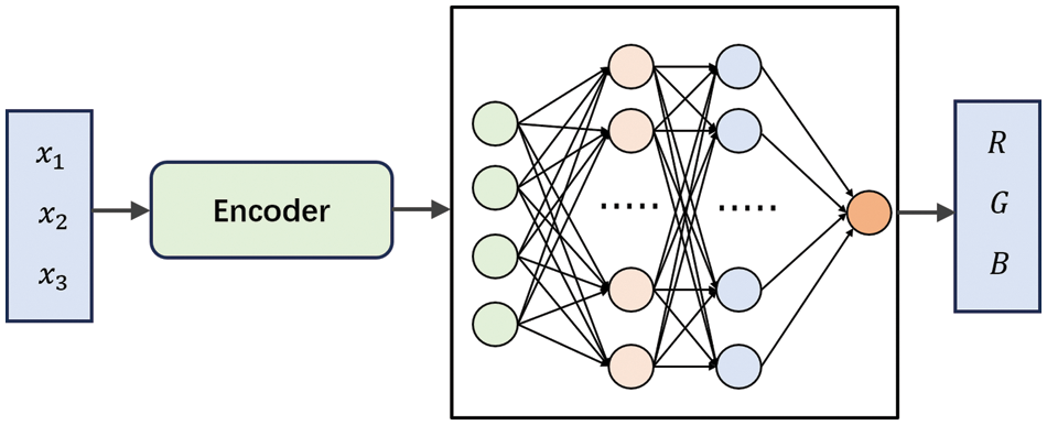
Figure 1: Implicit neural representations

NeRF also falls into the category of INR, which trains coordinate-based networks to approximate the continuous radiance fields within the volume enclosed by the object’s surface. Once the training is completed, NeRF enables rendering 2D images from any new viewing directions. As one of the most significant breakthroughs in INRs, NeRF has attracted enormous interest since its inception. Mip-NeRF [24] addresses the issue of ignoring the volume and size of the observed region in NeRF by replacing rays with cones, allowing for sampling from a continuous conical frustum instead of discrete points. Instant-NGP [25] improves upon existing graphics structures and applies them to volumetric rendering frameworks by utilizing a sparsely parameterized voxel grid as a scene representation and optimizing both the scene and MLP (where one MLP serves as the decoder) based on gradients, thereby accelerating the transition from 2D to 3D reconstruction. PixelNeRF [26] incorporates spatial image features aligned with each pixel as input, leveraging convolutional networks to extract low-level features, which are then combined with the input to the NeRF grid to learn prior knowledge about the scene. This approach allows for generating new views with minimal input, even for unknown scenes. FiG-NeRF [27] interprets scenes as a geometrically consistent background and a deformable foreground representing object categories. By using only optical supervision and randomly captured object images, accurate 3D object category models can be learned.

2.2 Physics Informed Neural Networks in CFD

Over the past few decades, significant progress has been made in the field of Computational Fluid Dynamics (CFD) (as shown in Fig. 2) [28] for solving compressible or incompressible flow problems [29] using mesh-based numerical methods such as finite volume methods and finite element methods [30]. Nevertheless, the generation of polygonal grids is a time-consuming task, and solving inverse problems is intractable. Deep learning seems to be a promising tool for data-driven computational mechanics [31,32] (Fig. 3). For example, a pioneering work can be seen in Milano et al. [33], who proposed a nonlinear neural network that significantly increased the prediction accuracy of near-wall velocity fields. However, different from the fields of object detection and tracking, where deep learning has been applied successfully, complex fluid flow possesses highly nonlinear and multiscale characteristics, and the data are often sparse and noisy, which poses great challenges to the pure data-driven paradigm of computing science.

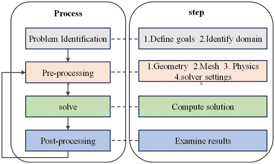
Figure 2: Computational fluid dynamics

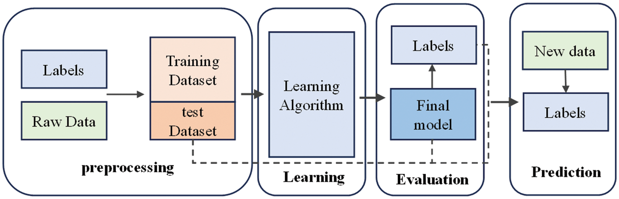
Figure 3: Machine learning

Physics-Informed Neural Network [6,34] addressed the aforementioned issue by informing neural networks of the physical mechanisms of fluid dynamics. In addition to penalizing the deviation of neural network predictions from data, PINNs incorporate the residual of Navier-Stokes equations and boundary conditions into loss terms. Once trained, the PINN can quickly make predictions and thus can be used as a surrogate model. Furthermore, due to the differentiability of PINN, it is an ideal choice for solving inverse and optimization problems. It is noteworthy that classical CFD algorithms [35] still maintain their advantages in accuracy and efficiency when solving standard forward problems and meet the practical requirements of robustness and computational efficiency in many applications. Therefore, classical methods and deep neural network methods will coexist and complement each other in the foreseeable future.

2.3 Fluid Reconstruction Based on RGB Images

Fluid flow patterns (e.g., color, density, and velocity) can be analyzed by visualizing and tracking the movement of passive tracers such as ink or dye in the fluids. Experimental fluid mechanics widely adopts Particle Image Velocimetry (PIV) [36], which is a non-intrusive laser optical measurement technique where the velocity field of an entire region within the flow is measured simultaneously. However, PIV requires cumbersome configuration of experimental devices and the accuracy has not matured to a satisfactory level in 3D. To alleviate the difficulty, Gregson et al. [37] reconstructed fluids from RGB images by combining fluid capture, simulation, and proximal methods [38] based on global priors. Zang et al. [39] extended the visible light tomographic imaging technique with sparse viewpoints to achieve fluid flow reshaping, utilizing interpolation techniques and two novel regularization methods. Qiu et al. [40] employed convolutional networks to simulate input scenes with flexible coupling effects based on the estimated velocity field, resulting in stable image effects. Chu et al. [11] propose the first method for combining NeRF and PINN to recover the density and velocity of fluids from sparse multi-view RGB video streams.

2.4 Uncertainty Quantification in Deep Neural Networks

Uncertainty is ubiquitous in science and has a profound impact on engineering design and modeling [41–44]. Many approaches have been proposed for quantifying uncertainties of the prediction by deep neural networks, such as single deterministic methods [45], Bayesian methods [46], Test-time augmentation methods [47], and ensemble methods, as shown in Fig. 4 [48]. Single deterministic methods can be further categorized into internal uncertainty quantification methods and external uncertainty quantification methods, which involve modeling a single network and incorporating additional components on the network’s predictions to provide uncertainty estimation. Bayesian methods treat the weights of neural networks as random variables and make predictions based on multiple sets of weight distributions. Test-time augmentation methods apply data augmentation techniques to create multiple test samples for each test sample and compute the prediction distribution to measure uncertainty. Ensemble methods combine prediction results from multiple members of an ensemble to quantify uncertainty. While ensemble methods require high memory usage, they offer advantages in simplicity, scalability, and flexibility.

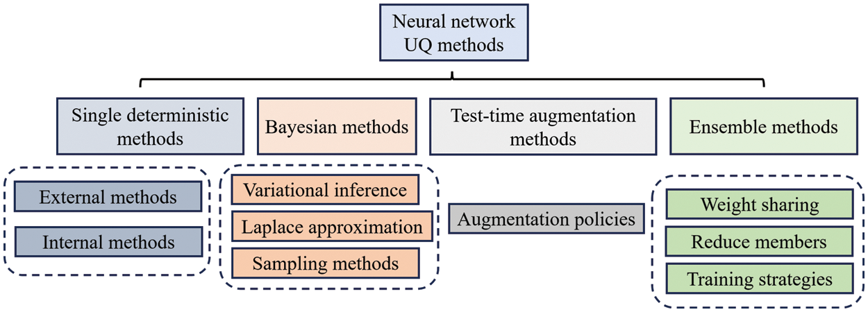
Figure 4: Uncertainty estimation in deep neural network

3  Method

3.1 Fluid Neural Representation Based on FreeNeRF

As a differentiable volume rendering approach, NeRF uses fully connected neural networks to construct a mapping from Cartesian coordinates and viewing directions to color intensities c and optical densities ρ in a 3D scene (Fig. 5):

F(x,y,z,θ,ϕ)→(c,ρ)(1)

where (x, y, z) denotes the coordinates in the three-dimensional Cartesian coordinate system, color c=(r,g,b) consists of three components associated with RBG channels, and (θ,ϕ) represents the azimuthal and polar angles of viewing directions. Supervised by the data of 2D images from different viewpoints, two Multilayer Perceptrons (MLPs) in NeRF, one coarse and one refined, are trained jointly to synthesize novel view images. It is noted that in Chu’s paper [11], the view direction variables (θ,ϕ) are neglected for simplicity, based on the assumption of Lambertian surfaces and isotropic scattering medium. By adding the time dimension, the model can be extended to the dynamics of fluid scenes in both spatial and temporal dimensions:

Fs:(x,y,z)→(c,ρ)Fd:(x,y,z,t)→(c,ρ)(2)

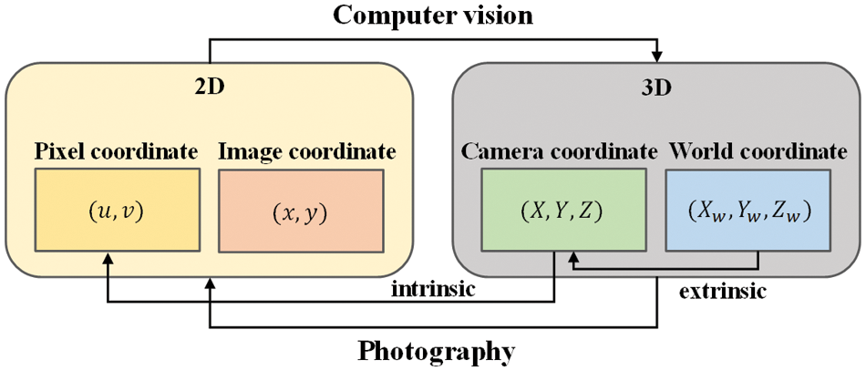
Figure 5: Schematic of camera model

The aforementioned spatiotemporal neural radiance fields learn the information from neural scene flow [49]. By predicting 3D scene flow for both forward and backward frames, it represents the 3D displacement vectors of the x position at time i + 1 and i − 1.

Fi=(Fi→i+1,Fi→i−1)(3)

This is based on the hypothesis that the color of a pixel obtained by volume rendering at time i should be the same as the color of the pixel reached by the ray after moving to a new coordinate at time j.

Further, with the given volume density and color function, it is possible to use the volume rendering function to obtain the color C(r) for any camera ray r(t)=o+td, in which o represents the camera position, and d denotes the viewing direction,

C(r)=∫t2t1T(t)⋅ρ(r(t))⋅c(r(t),d)⋅dt(4)

where T(t) represents the cumulative transmittance, which denotes the probability of a ray propagating from t1 to r without being intercepted. It can be calculated using the following equation:

T(t)=exp⁡[−∫t1tρ(r(s))⋅ds](5)

By tracing camera rays C(r) passing through each pixel in the target synthesized image, novel views can be generated. This integration can be evaluated numerically with non-deterministic stratified sampling, where rays are partitioned into N equally spaced intervals, and samples are drawn uniformly from each interval. Then, Eq. (5) can be approximated as follows:

C^(r)=∑i=1NαiTiciTi=exp⁡[−∑j=1i−1ρjδj](6)

where δi represents the distance from sample i to sample i+1, (ρi,ci) are the density and color evaluated at sampling point i along the given ray, respectively, which are computed by the neural network, and αi is given by the following equation:

αi=1−exp⁡(ρiδi)(7)

In general, the expected depth of a ray can be calculated by utilizing the cumulative transmittance:

d(r)=∫t2t1T(t)⋅ρ(r(t))⋅t⋅dt(8)

The above equation can be achieved by approximating Eqs. (3) and (5) in a similar way to Eq. (6).

D^(r)=∑i=1NαitiTi(9)

For each pixel, the square error photometric loss is used to train neural network parameters. Over the whole image, this is given by the following equation:

ℒ=∑r=R‖C^(r)−Cg(r)‖22(10)

where ℒ is a batch of rays associated with the image to be synthesized, and Cg(r) is the true color of the training image pixel associated with R.

Position encoding is a commonly used technique in NeRF to improve the reconstruction of fine details in rendered views [9] (Fig. 6). The following position encoding γ is applied to each component of the scene coordinates x (normalized to [−1, 1]):

γL(x)=(sin⁡(20x),cos⁡(20x),sin⁡(21x),cos⁡(21x),...,sin⁡(2L−1x),cos⁡(2L−1x))(11)

where L is a user-determined coding dimension parameter, and in the original NeRF paper, x was set to L=10, and d was set to L=4.

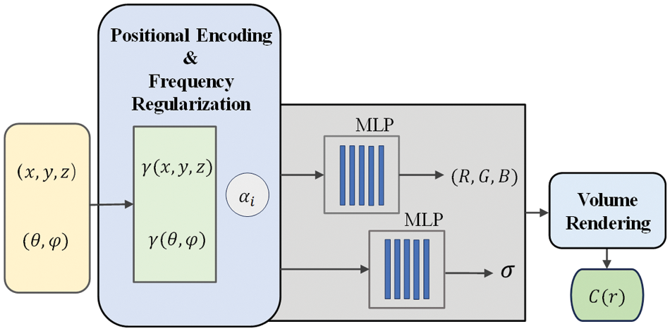
Figure 6: Schematic of neural radiance field

A significant challenge faced by the basic NeRF structure is the tendency to overfit training data, thereby limiting their ability to interpret three-dimensional geometry in a multi-view manner. One possible reason is that position encoding, which extends the input location information to higher dimensions, prevents the NeRF from exploring low-frequency information in the early stages of neural network training. Based on the work of Chu et al. [11], we adopt frequency regularization proposed by Yang et al. [15] in FreeNeRF to optimize the reconstruction of sparse view inputs for smoke. This approach improves the position encoding by using a linearly growing frequency mask to modulate the visible spectrum based on training time steps. The formula is given as follows:

γ′L(t,T;x)=γL(x)⊙α(t,T,L)with αi(t,T,L)={1t⋅LT−⌊t⋅LT⌋0ifi≤t⋅LT+3ift⋅LT+3<i≤t⋅LT+6ifi>t⋅LT+6(12)

in which t and T represent the current training iteration and the final iteration, respectively. The frequency regularization mitigates the instability and vulnerability to high-frequency signals at the beginning of training and gradually provides NeRF with high-frequency information to avoid excessive smoothing.

3.2 Fluid Velocity Estimation by Residual PINN

PINNs encode physical laws represented by Partial Differential Equations (PDEs) in neural networks by transforming PDEs to an optimization model that minimizes a loss function containing the residuals (Fig. 7). In its most general form, a PDE can be expressed as follows:

F(φ(z);γ)=f(z),in ΩB(φ(z))=g(z),on ∂Ω(13)

where Ω⊂Rd is the domain on which the physical problem is defined, ∂Ω indicates the boundary of the domain, z:=[x1,...,xd−1;t] denotes the spatio-temporal coordinates, u represents the unknown physical fields, γ is a physical parameter, f is a function that identifies the problem data, and ℱ is the nonlinear differential operator. In the second equation, ℬ is expressed as an operator with arbitrary initial or boundary conditions associated with the problem, and g is taken to be a boundary function. Eq. (13) can be used in forward and backward problems. The goal of the forward problem is to find a function u for each z when γ is given. In the case of the inverse problem, γ must also be determined from the data.

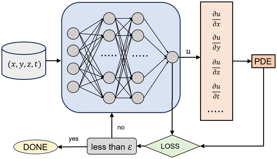
Figure 7: A brief schematic of PINN

To solve Eq. (13), ϕ(z) can be approximated with a neural network that is parameterized by a set of parameters θ,

φ(z)≈φ^θ(z)(14)

where θ is obtained by minimizing a loss function that depends on the observed data and PDEs as well as the boundary conditions.

θ∗=arg⁡minθ⁡(wℱℒℱ(θ)+wℬℒℬ(θ)+wdℒdata(θ))(15)

As can be seen from the above equation, PINN differs from traditional neural networks in that the residuals of PDEs are introduced into the loss function to enforce physical laws, whereby the accuracy and efficiency can be enhanced even with sparse training data.

Based on the model structure used in Chu’s paper [11], the architecture of our neural networks is shown in Fig. 8, which contains residual structure [50] and two-layer activation function from sf-PINN [51]. Residual networks address the issue of “degradation” in NNs by incorporating the original features into the subsequent training process, thereby avoiding feature loss during training. The definition of a residual network is very simple and is given by the following equation:

f(x)=g(x)+x(16)

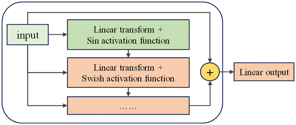
Figure 8: Residual structure and two-layer activation function

Moreover, sf-PINN and its double-layer activation function have been proven to effectively increase gradient variability, preventing training stagnation and getting trapped in local minima. They have shown good performance in various forward and inverse modeling problems. The sin [23] and Swish functions [52] (as shown in Fig. 9) are defined by the following equation:

f(x)=sin⁡(x)f(x)=x⋅η(x) with η(x)=11+e−x(17)

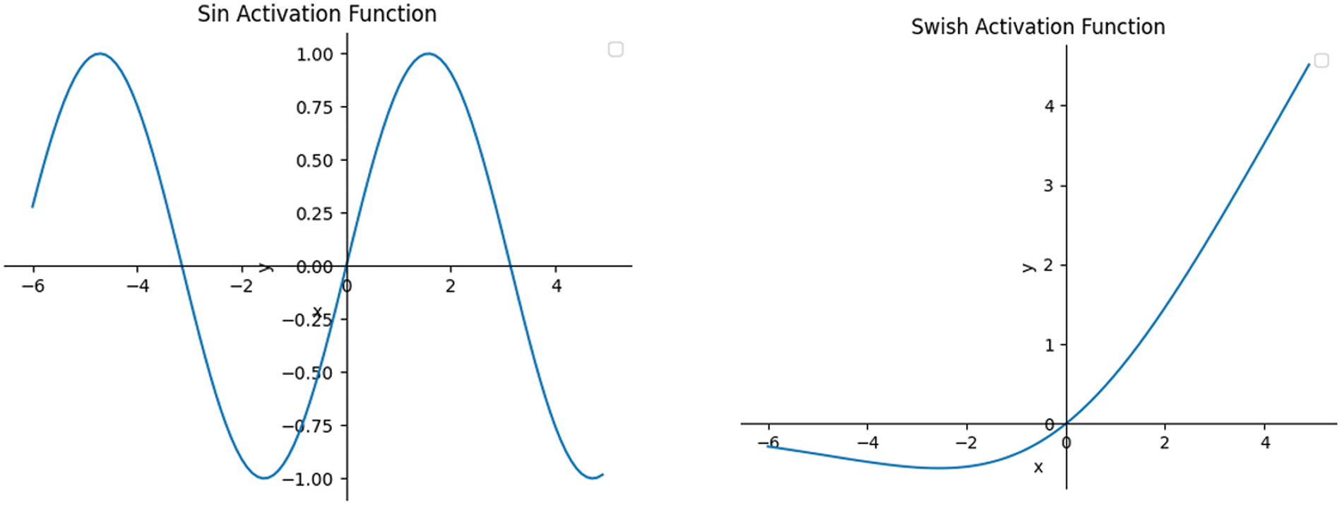
Figure 9: Schematic of activation function

The flow of incompressible fluid is governed by the Navier-Stokes equation [53]:

∂u∂t+u∇⋅u=−ρ∇p+1Re∇2u+b (momentum equation)∇⋅u=0 (incompressibility)(18)

where u is the velocity, which contains three components (ux,uy,uz), p is the pressure, Re is Reynolds number, and b is the body force.

The particles (passive scalar) in fluids are transferred through convection and diffusion processes, which are characterized by the convection-diffusion equation:

∂c∂t+u⋅∇c=0(19)

where c is the mass concentration of smoke particles, which is proportional to optical density ρ. In the remainder of the paper, we will not distinguish between c and ρ. Based on the particle density distribution obtained from NeRF, a PINN is trained to construct a mapping Fv spatio-temporal coordinates to velocity:

Fv:(x,y,z,t)→u(ux,uy,uz)(20)

which minimizes the following loss terms:

ℒDcDt=(∂c∂t+u⋅∇c)2,ℒNSE=‖∂u∂t+u⋅∇u‖22+wdiv‖∇⋅u‖22(21)

We take the partial derivatives of the velocity components obtained from the operations via the FFJORD tool [54] and encode them from the Navier-Stokes equations into the PDE loss function, which is added to each gradient backpropagation of the neural network. thus incorporating a physical prior in the hybrid model. The merit of PINN is that the approach does not require boundary conditions as input and can handle fluid within arbitrary spatial regions. In other words, we train a velocity network based on PINN.

3.3 NeRF Ensembles and Uncertainty Analysis

In the field of computer vision, there are two main types of uncertainties: aleatoric uncertainty and epistemic uncertainty [14]. Aleatoric uncertainty arises from the inherent uncertainty in the input data, while epistemic uncertainty refers to the uncertainty in the model weights learned. Despite being one of the preferred methods for numerous computer vision modeling tasks, most existing models of NeRF are not able to accurately quantify their inherent model uncertainties (epistemic uncertainties).

Ensemble learning combines multiple base models to fulfill learning tasks. It is commonly perceived as a meta-algorithm and is rooted in intuitive thinking. it provides a representation of model uncertainty in predictions by quantifying the prediction distribution derived from multiple constituent members and evaluating the diversity among member predictions. This framework can be readily implemented and deployed without needing any alterations to the underlying NeRF and PINN architectures.

Since the primary application of NeRFs is to generate two-dimensional images of novel viewpoints, the uncertainty in color prediction is the issue that needs to be addressed first (Fig. 10). In accordance with the theory of ensemble learning, we train multiple NNs [55] {fθn}n=1...N. They are trained on the same dataset but initialized with different weights. The final prediction is obtained by averaging the predictions of all member networks. Hence, the expected color of r (ray) in the scene is written as:

C¯(r)=1N∑n=1NCθn(r)(22)

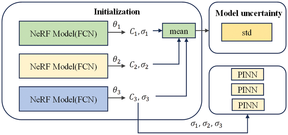
Figure 10: Uncertainty analysis based on ensembles learning

The average amount of variability is represented by the standard deviation (std) of individual members’ predictions as:

σRGB(r)=1N∑n=1N(C¯(r)−Cθn(r))2(23)

By employing this intuitively feasible approach, we obtain a color-density distribution field predicted by a neural network ensemble. These distributions are mutually independent and can be accessed independently in time. This ensemble learning-based framework can be easily extended and applied to NeRF-based models.

Based on the above equation, we can directly assess the use of C¯(r) and σRGB(r) to analyze uncertainty. However, the above equations are obtained for each individual color channel, to simplify the calculation and analysis, we calculate the average standard deviation of the three color channels:

σ¯RGB(r)=13∑i∈{R,G,B}σRGB,i(r)(24)

where σRGB,i(r) represents the standard deviation on each RGB color channel.

Although NeRF can manipulate the geometric shape, color, and density distribution of 3D objects or scenes, it fails to provide information on invisible physical quantities such as velocity and pressure, which are crucial for engineering design in fluid dynamics. Chu et al. [11] proposed to employ PINN to infer the velocity fields according to the densities obtained by NeRF. Because the fluid flow model is coupled with the particle transportation model, the accuracy of PINN in predicting velocity is closely linked with the uncertainty of the density distribution of the particles. With a similar stacked training approach, the distribution of the velocity field is evaluated by training multiple PINNs under the same conditions:

σu,i(ρ)=1N∑n=1N(ui(ρ)−u¯i(ρ))2  i=x,y,z(25)

where i represents the three components of velocity, and we adopt the mean of these three standard deviations as the final uncertainty term.

The work of PINN can also be accomplished using a multi-output approach, as shown in Fig. 11, which has been tested in experiments. In order to maintain consistency within the framework, an integrated training method is employed in subsequent discussions. Regardless of which method is used, we obtain the predicted distribution of the velocity field, which enables an in-depth analysis of it.

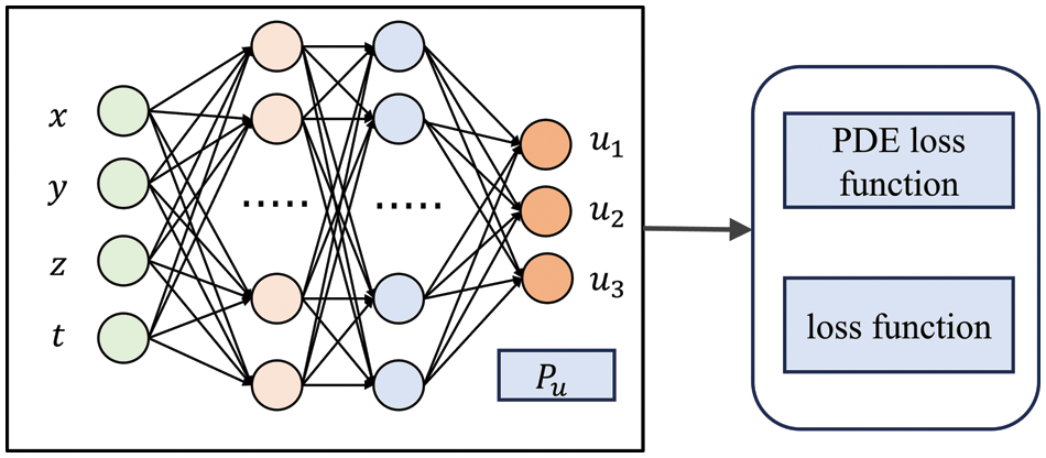
Figure 11: Neural network with multiple outputs

4  Results and Evaluation

4.1 Fluid Reconstruction Results

The present work adopts the ScalarFlow dataset [56], which comprises real-world smoke plumes captured by five fixed cameras positioned along a 120-degree arc. In this dataset, each fixed view comprises 120 frames with a duration of about 4 s. During training, the video frame is split into 600 images. In each training iteration, an image is selected randomly, and by utilizing the time anchor present in the image, the neural network predicts the attributes of the spatial point within the current scene. Although only 1024 pixel points were sampled at a time and fed into the neural network for training, the large number of training iterations (600 k) ensured that each pixel in the image was used at least once. The machine parameters used for training our model are outlined below:

•   Processor: Intel Core i9-10900x @ 3.70 GHz

•   RAM: 64 GB DDR4 RAM

•   GPU: NVIDIA GeForce RTX 3090

•   Hard-Disk Drive: 1 TB SSD + 3 TB HDD

We rendered the smoke plumes generated by the hybrid model into a 30-frame (1-s) RGB video, covering the entire process from smoke appearance to generation. Fig. 12 presents representative video frames extracted and arranged in chronological order (original dataset images on the left, rendered images on the right). It can be observed that the generated model not only achieves high fidelity in static images but also captures temporal dynamics features. In addition, some challenges arise in the rendering process. For example, spatial points that are close to white are rendered as pure white in the new view, as shown in Fig. 13. This is possibly due to flaws in the volume rendering itself as well as the repeated use of estimation in the calculation process. This necessitates more reasonable regularization penalty conditions in our future work.

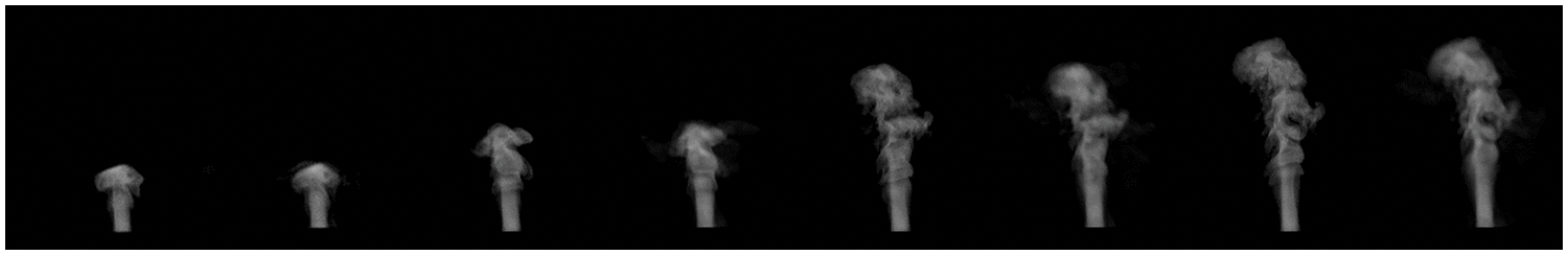
Figure 12: Five intercepted video frames in the rendering result

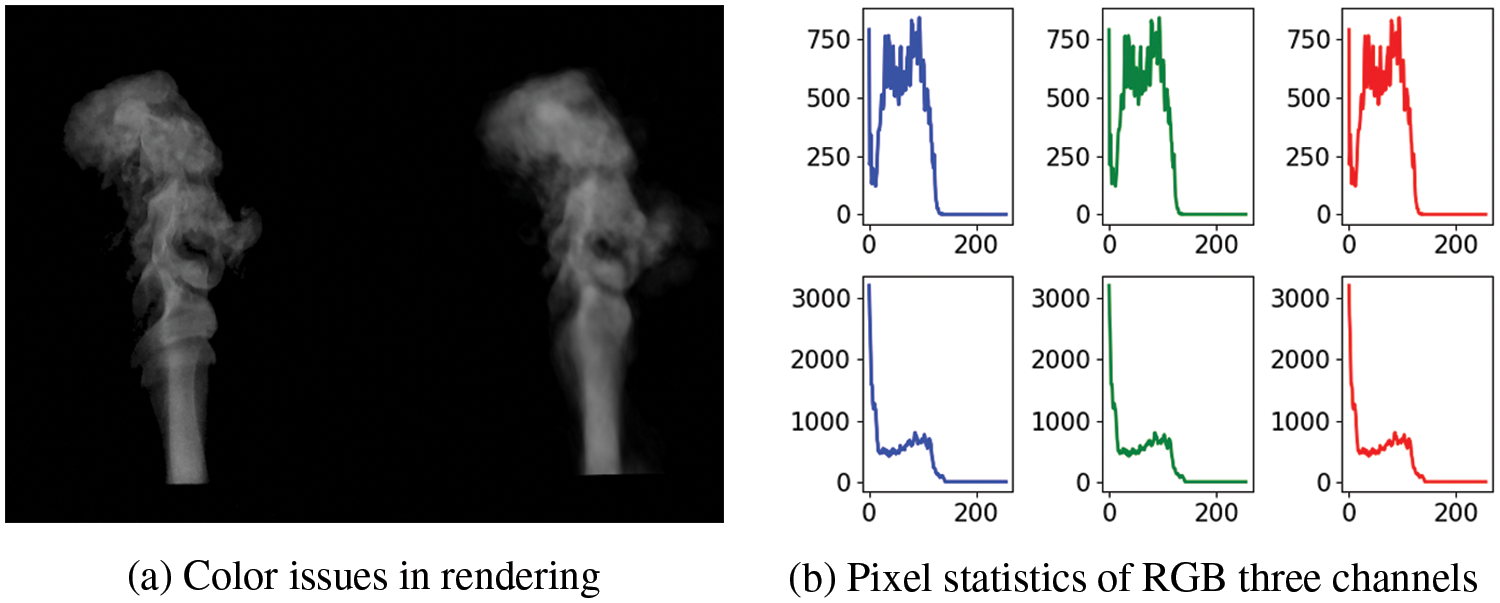
Figure 13: Problems we encountered

As the velocity is invisible to the naked eye, we convert the acquired velocity and vorticity into the HSV space and render it as an RGB image, as shown in Fig. 14. Vorticity is used to describe the local rotation of a fluid parcel, which is the spin of an air microcluster in the atmosphere. As can be seen from the image, the velocity field obtained through PINN is non-linear and has been captured by our algorithm.

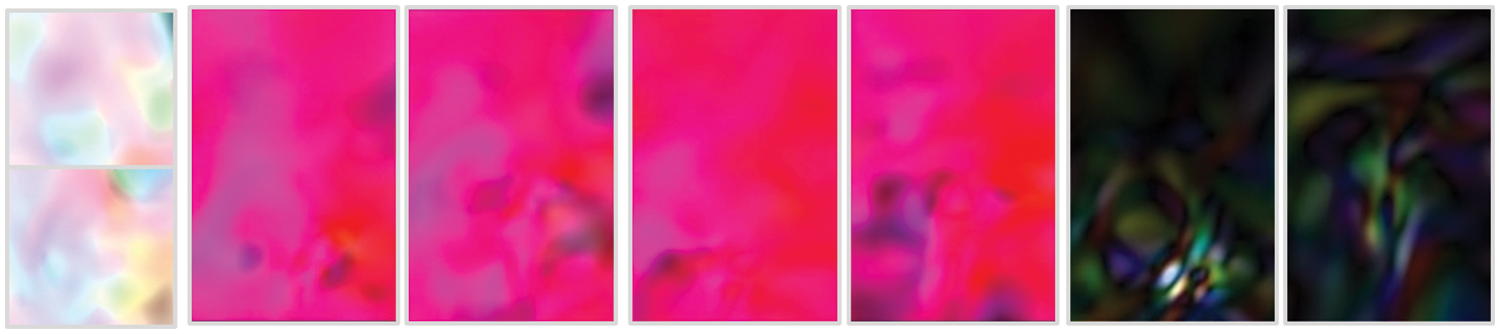
Figure 14: Velocity/Vorticity (rgb images)

Common quality assessment metrics, such as PSNR, SSIM, and LPIPS, are often used. In this paper, we adopted PSNR [57] as the criterion for evaluating the quality of generated images with original training images, given by the following equation:

PSNR(I)=10⋅log10(MAX(I)2MSE(I))(26)

A comparison was made between our rendered results and Chu’s model [11] using the test set. The Fig. 15 below showcases the juxtaposition of six randomly selected images from the training data in chronological order with the test results obtained through PSNR evaluation. On the right side, the velocity loss data from the final 10k training iterations are presented. It is evident that our rendered results demonstrate certain enhancements in terms of fine details at the same number of iterations. Furthermore, the training process of the velocity network weights exhibits a higher level of stability.

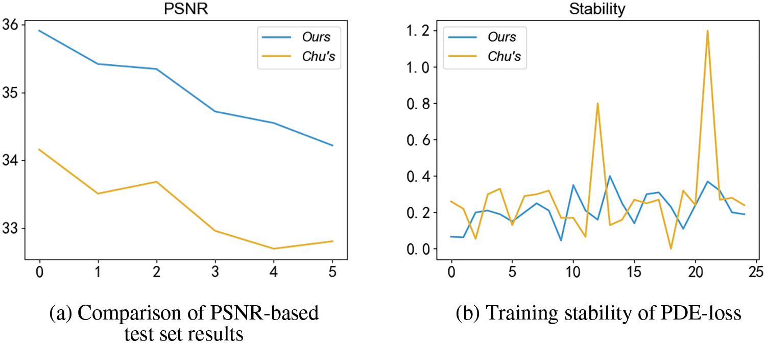
Figure 15: Model comparison

4.2 Uncertainty Analysis Results

We first examine the accuracy of color predictions for points in space along specific directions. A statistical analysis was performed on four sets of training samples collected over time (10, 100, 250, 500 k), as depicted in Fig. 16. Fig. 16 (left) features a line chart exhibiting the standard deviations for each batch of 1024 training points (sorted for improved clarity, as image oscillation was present), while Fig. 16 (right) showcases the distribution range of standard deviations. The figure illustrates that the maximum standard deviation predicted by the model is approximately 0.2, with the majority of values falling below 0.1. From Fig. 13, it can be seen that the values predicted by neural network for smoke particles are mostly approaching to 0. This implies that while the absolute value of uncertainty is not particularly high, there still exists a notable level of uncertainty relative to the mean prediction.

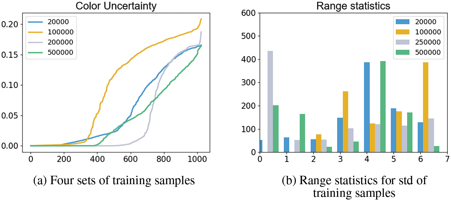
Figure 16: Color uncertainty

Furthermore, the pie chart (Fig. 17) also demonstrates that as the number of training iterations increases, there is an overall decrease in the model’s predicted uncertainty (the left corresponds to 100 k iterations, while the right corresponds to 600 k iterations). This indicates that although each training instance captures images at different instances of time, the color of a specific point in the dynamic fluid spatial domain could be similar or exhibit negligible changes over time.

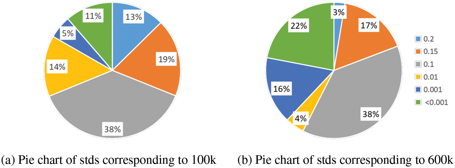
Figure 17: Color uncertainty—pie chart

To examine the accuracy of the aforementioned observation, we constructed a box plot for the standard deviations of the predicted results, ranging from 10 to 600 k with an increment of 100 k, as depicted in Fig. 18. The box plot is a statistical chart used to display the dispersion of a set of data. It is primarily used to reflect the distribution characteristics of raw data, and can also be employed to compare the distribution characteristics of multiple data sets. The observed trend from the graph indicates that there is no evident variation in the minimum and maximum values, with outliers close to 0.2 present even at the 600k-th training iteration. However, a declining trend in the overall standard deviation can be observed from the quartiles utilized to construct the box.

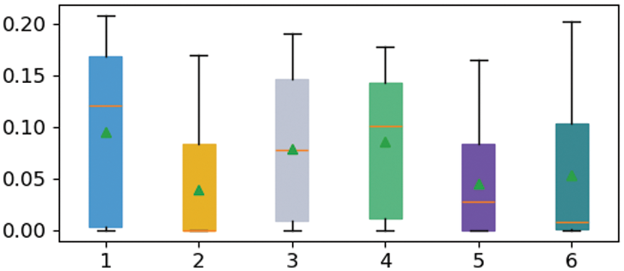
Figure 18: Color uncertainty—box plot

The optical density ρ at a specific spatial point obtained by NeRF indicates its opacity or high scattering characteristics of the object at that point (e.g., clouds or fog). The optical density is linearly proportional to the mass concentration of smoke particles, thus reflecting the transfer of particles in fluid flow. Due to the uncertainty in NeRF training, the number of density points in the fluid model will be different. In the simultaneously trained NeRFs, we first statistically analyze the density values as an initial quantification criterion for the density uncertainty. From Fig. 19, it can be observed that statistical analysis was performed on the density quantity six times, ranging from 100 to 600 k. The differences in each iteration are attributed to differences in scene selection.

As can be seen in Fig. 19, the values of densities at 200 and 600 k iterations are higher. We quantified the uncertainty (standard deviation) for these two instances separately. According to Fig. 20, we can infer that overall, density-related uncertainty has decreased. However, due to lack of supervision, there still remains a significant level of uncertainty even with an adequate number of training iterations.

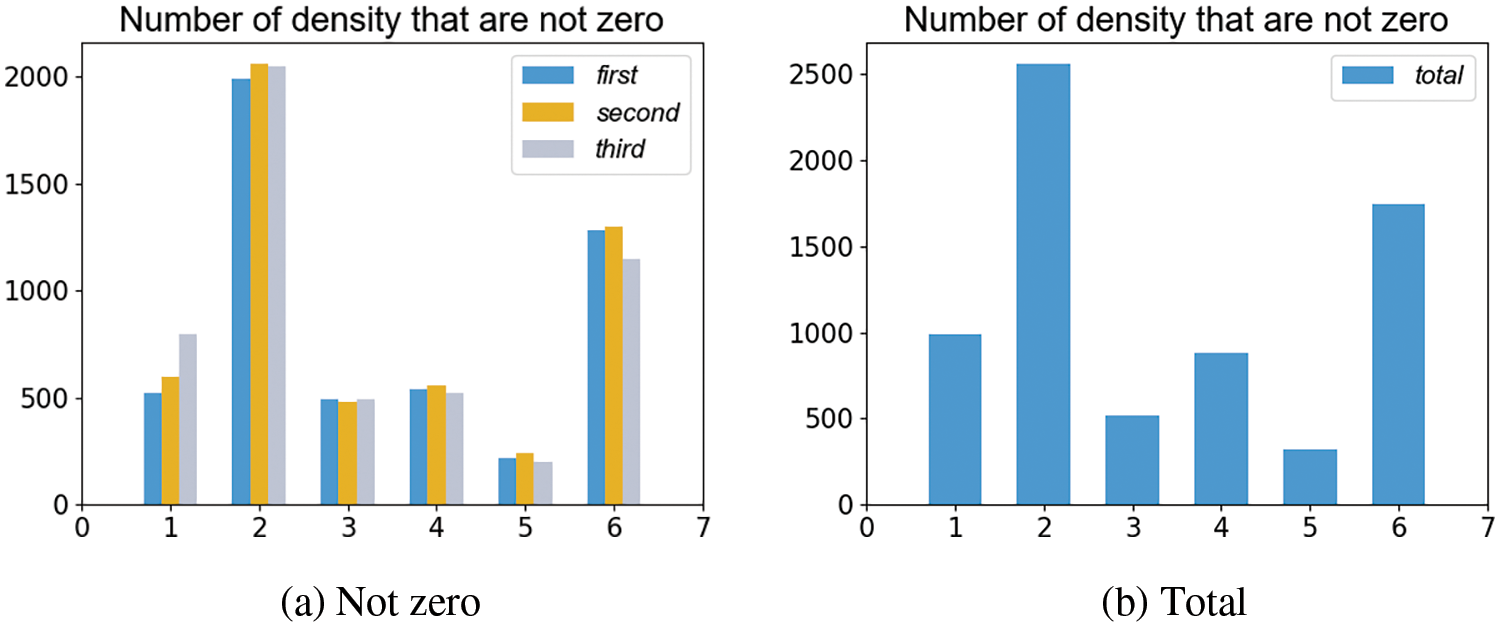
Figure 19: Density uncertainty

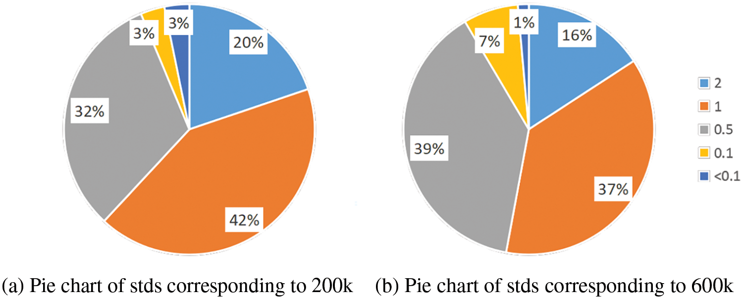
Figure 20: Density uncertainty—pie chart

Finally, we quantified velocity uncertainty, which stems from the uncertainty in neural network weight learning and the uncertainty in density distribution. As shown in Table 1, it is the mean value of the velocity we measured during training. From Fig. 21, it can be observed that the overall trend of velocity uncertainty increases as the number of iterations increases. Moreover, from Fig. 21b, it can be noted that since the mean velocity is only between 0.01–0.5, the uncertainty in velocity compared to color, which has clear dataset supervision, requires further extension of supervised training in future work.

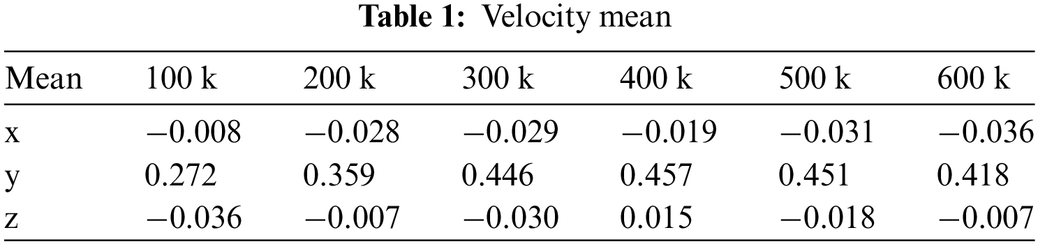
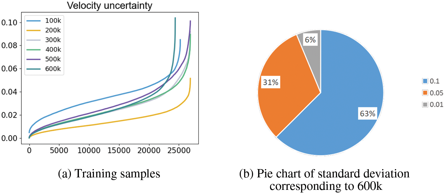
Figure 21: Velocity uncertainty

5  Conclusion

In the context of smoke reconstruction from 2D images with NeRF and PINN, we introduce an ensemble learning-based framework for evaluating uncertainties of color, density, and velocity fields. The color and density uncertainties are computed by training multiple NeRF models, and the velocity uncertainties are evaluated through multiple PINNs with different density inputs. To enhance the image quality, we employ frequency regularization in NeRF and add residual blocks and two-layer activation functions to PINN. The proposed framework facilitates uncertainty quantification within an end-to-end dynamic smoke model and demonstrates remarkable stability and scalability, which is of significance to downstream tasks including reliability analysis, engineering design, object segmentation, etc. In the future, we will apply the framework to a wide range of engineering applications, such as robust structural optimization of fluid channels, object detection and segmentation, robotic visual perception, etc. Besides, we will investigate the feasibility of adapting the present uncertainty quantification algorithm to acoustic and electromagnetic fields [31,58].

Acknowledgement: The authors appreciate the help of Dr. Zhongming Hu in fluid mechanics.

Funding Statement: This study was funded by the National Natural Science Foundation of China (NSFC) (No. 52274222) and research project supported by Shanxi Scholarship Council of China (No. 2023-036).

Author Contributions: Study conception and design: H. Lian, L. Chen, S. Li, Q. Hu; data collection: J. Wang, Q. Hu, R. Cao, P. Zhao; analysis and interpretation of results: H. Lian, J. Wang, S. Li, R. Cao; draft manuscript preparation: H. Lian. J. Wang, L. Chen, R. Cao. All authors reviewed the results and approved the final version of the manuscript.

Availability of Data and Materials: Below are very concise guidelines for generating synthetic scenes: To generate a new synthetic scene, it is imperative to create a simulation script for the scene (Step 1). Render the scene using Blender (Step 2). Write code to appropriately export camera poses (Step 3). Adjust the code, to load the image sequences along with the camera poses.

Conflicts of Interest: The authors declare that they have no conflicts of interest to report regarding the present study.

References

1. LeCun, Y., Bengio, Y., Hinton, G. (2015). Deep learning. Nature, 521(7553), 436–444. [Google Scholar] [PubMed]

2. Cheng, R., Yin, X., Chen, L. (2022). Machine learning enhanced boundary element method: Prediction of Gaussian quadrature points. Computer Modeling in Engineering & Sciences, 131(1), 445–464. https://doi.org/10.32604/cmes.2022.018519 [Google Scholar] [CrossRef]

3. Shen, X., Du, C., Jiang, S., Sun, L., Chen, L. (2023). Enhancing deep neural networks for multivariate uncertainty analysis of cracked structures by POD-RBF. Theoretical and Applied Fracture Mechanics, 125, 103925. [Google Scholar]

4. Chen, L., Zhao, J., Lian, H., Yu, B., Atroshchenko, E. et al. (2023). A BEM broadband topology optimization strategy based on Taylor expansion and SOAR method–Application to 2D acoustic scattering problems. International Journal for Numerical Methods in Engineering, 124(23), 5151–5182. [Google Scholar]

5. Kutz, J. N. (2017). Deep learning in fluid dynamics. Journal of Fluid Mechanics, 814, 1–4. [Google Scholar]

6. Raissi, M., Perdikaris, P., Karniadakis, G. E. (2019). Physics-informed neural networks: A deep learning framework for solving forward and inverse problems involving nonlinear partial differential equations. Journal of Computational Physics, 378, 686–707. [Google Scholar]

7. Jasak, H. (1996). Error analysis and estimation for the finite volume method with applications to fluid flows. https://www.croris.hr/crosbi/publikacija/ocjenski-rad/445133 (accessed on 31/12/1996). [Google Scholar]

8. Feng, K., Shi, Z. C. (1996). Finite element methods. In: Mathematical theory of elastic structures, pp. 289–385. Berlin, Heidelberg: Springer. [Google Scholar]

9. Mildenhall, B., Srinivasan, P. P., Tancik, M., Barron, J. T., Ramamoorthi, R. et al. (2021). NeRF: Representing scenes as neural radiance fields for view synthesis. Communications of the ACM, 65(1), 99–106. [Google Scholar]

10. Phang, J. T. S., Lim, K. H., Chiong, R. C. W. (2021). A review of three dimensional reconstruction techniques. Multimedia Tools and Applications, 80(12), 17879–17891. [Google Scholar]

11. Chu, M., Liu, L., Zheng, Q., Franz, E., Seidel, H. P. et al. (2022). Physics informed neural fields for smoke reconstruction with sparse data. ACM Transactions on Graphics, 41(4), 1–14. [Google Scholar]

12. Shen, J., Ruiz, A., Agudo, A., Moreno-Noguer, F. (2021). Stochastic neural radiance fields: Quantifying uncertainty in implicit 3D representations. 2021 International Conference on 3D Vision (3DV), London, UK, IEEE. [Google Scholar]

13. Shen, J., Agudo, A., Moreno-Noguer, F., Ruiz, A. (2022). Conditional-flow NeRF: Accurate 3D modelling with reliable uncertainty quantification. European Conference on Computer Vision, Switzerland, Springer. [Google Scholar]

14. Gawlikowski, J., Tassi, C. R. N., Ali, M., Lee, J., Humt, M. et al. (2023). A survey of uncertainty in deep neural networks. Artificial Intelligence Review, 56(Suppl 1), 1513–1589. [Google Scholar]

15. Yang, J., Pavone, M., Wang, Y. (2023). FreeNeRF: Improving few-shot neural rendering with free frequency regularization. Proceedings of the IEEE/CVF Conference on Computer Vision and Pattern Recognition, Vancouver, Canada. [Google Scholar]

16. Strümpler, Y., Postels, J., Yang, R., Gool, L. V., Tombari, F. (2022). Implicit neural representations for image compression. European Conference on Computer Vision, Switzerland, Springer. [Google Scholar]

17. Osher, S., Fedkiw, R., Osher, S., Fedkiw, R. (2003). Constructing signed distance functions. In: Level set methods and dynamic implicit surfaces, pp. 63–74. New York, NY, USA: Springer. [Google Scholar]

18. Tiwari, G., Antić, D., Lenssen, J. E., Sarafianos, N., Tung, T. et al. (2022). Pose-NDF: Modeling human pose manifolds with neural distance fields. European Conference on Computer Vision, Switzerland, Springer. [Google Scholar]

19. Sun, K., Wu, S., Huang, Z., Zhang, N., Wang, Q. et al. (2022). Controllable 3D face synthesis with conditional generative occupancy fields. Advances in Neural Information Processing Systems, 35, 16331–16343. [Google Scholar]

20. Sitzmann, V., Zollhöfer, M., Wetzstein, G. (2019). Scene representation networks: Continuous 3D-structure-aware neural scene representations. Advances in Neural Information Processing Systems 32 (NeurIPS 2019). [Google Scholar]

21. Niemeyer, M., Mescheder, L., Oechsle, M., Geiger, A. (2020). Differentiable volumetric rendering: Learning implicit 3D representations without 3D supervision. Proceedings of the IEEE/CVF Conference on Computer Vision and Pattern Recognition, pp. 3504–3515. [Google Scholar]

22. Saito, S., Huang, Z., Natsume, R., Morishima, S., Kanazawa, A. et al. (2019). PIFu: Pixel-aligned implicit function for high-resolution clothed human digitization. Proceedings of the IEEE/CVF International Conference on Computer Vision, Long Beach, CA, USA. [Google Scholar]

23. Sitzmann, V., Martel, J., Bergman, A., Lindell, D., Wetzstein, G. (2020). Implicit neural representations with periodic activation functions. Advances in Neural Information Processing Systems, 33, 7462–7473. [Google Scholar]

24. Barron, J. T., Mildenhall, B., Tancik, M., Hedman, P., Martin-Brualla, R. et al. (2021). Mip-NeRF: A multiscale representation for anti-aliasing neural radiance fields. Proceedings of the IEEE/CVF International Conference on Computer Vision. [Google Scholar]

25. Müller, T., Evans, A., Schied, C., Keller, A. (2022). Instant neural graphics primitives with a multiresolution hash encoding. ACM Transactions on Graphics, 41(4), 1–15. [Google Scholar]

26. Yu, A., Ye, V., Tancik, M., Kanazawa, A. (2021). pixelNeRF: Neural radiance fields from one or few images. Proceedings of the IEEE/CVF Conference on Computer Vision and Pattern Recognition, pp. 4578–4587. [Google Scholar]

27. Xie, C., Park, K., Martin-Brualla, R., Brown, M. (2021). Fig-NeRF: Figure-ground neural radiance fields for 3D object category. 2021 International Conference on 3D Vision (3DV), London, UK, IEEE. [Google Scholar]

28. Bhatti, M. M., Marin, M., Zeeshan, A., Abdelsalam, S. I. (2020). Recent trends in computational fluid dynamics. Frontiers in Physics, 8, 593111. [Google Scholar]

29. Constantin, P., Foias, C. (2020). Navier-stokes equations. Chicago, USA: University of Chicago Press. [Google Scholar]

30. Szabó, B., Babuška, I. (2021). Finite element analysis: Method, verification and validation. https://books.google.com.tw/books?hl=zh-CN&lr=&id=V_UqEAAAQBAJ&oi=fnd&pg=PP12&dq=Finite+element+analysis:+Method,+verification+and+validation&ots=Gqqk5KWQpf&sig=j6yGL-MwFeX4Hf7IlGkdcCSB3kw&redir_esc=y#v=onepage&q=Finite%20element%20analysis%3A%20Method%2C%20verification%20and%20validation&f=false (accessed on 28/05/2021). [Google Scholar]

31. Chen, L., Cheng, R., Li, S., Lian, H., Zheng, C. et al. (2022). A sample-efficient deep learning method for multivariate uncertainty qualification of acoustic-vibration interaction problems. Computer Methods in Applied Mechanics and Engineering, 393, 114784. [Google Scholar]

32. Wang, J., Sun, P., Chen, L., Yang, J., Liu, Z. et al. (2023). Recent advances of deep learning in geological hazard forecasting. Computer Modeling in Engineering & Sciences, 137(2), 1381–1418. https://doi.org/10.32604/cmes.2023.023693 [Google Scholar] [CrossRef]

33. Milano, M., Koumoutsakos, P. (2002). Neural network modeling for near wall turbulent flow. Journal of Computational Physics, 182(1), 1–26. [Google Scholar]

34. Karniadakis, G. E., Kevrekidis, I. G., Lu, L., Perdikaris, P., Wang, S. et al. (2021). Physics-informed machine learning. Nature Reviews Physics, 3(6), 422–440. [Google Scholar]

35. Zawawi, M. H., Saleha, A., Salwa, A., Hassan, N., Zahari, N. M. et al. (2018). A review: Fundamentals of computational fluid dynamics (CFD). AIP Conference Proceedings, vol. 2030. Tianjin, China, AIP Publishing. [Google Scholar]

36. Najjari, M. R., Hinke, J. A., Bulusu, K. V., Plesniak, M. W. (2016). On the rheology of refractive-index-matched, non-Newtonian blood-analog fluids for PIV experiments. Experiments in Fluids, 57, 1–6. [Google Scholar]

37. Gregson, J., Ihrke, I., Thuerey, N., Heidrich, W. (2014). From capture to simulation: Connecting forward and inverse problems in fluids. ACM Transactions on Graphics, 33(4), 1–11. [Google Scholar]

38. Bertsekas, D. P. (2011). Incremental proximal methods for large scale convex optimization. Mathematical Programming, 129(2), 163–195. [Google Scholar]

39. Zang, G., Idoughi, R., Wang, C., Bennett, A., Du, J. et al. (2020). Tomofluid: Reconstructing dynamic fluid from sparse view videos. Proceedings of the IEEE/CVF Conference on Computer Vision and Pattern Recognition, pp. 1870–1879. [Google Scholar]

40. Qiu, S., Li, C., Wang, C., Qin, H. (2021). A rapid, end-to-end, generative model for gaseous phenomena from limited views. In: Computer graphics forum, vol. 40, no. 6, pp. 242–257. Wiley Online Library. [Google Scholar]

41. Lian, H., Wang, Z., Hu, H., Li, S., Peng, X. et al. (2021). Monte Carlo simulation of fractures using isogeometric boundary element methods based on POD-RBF. Computer Modeling in Engineering & Sciences, 128(1), 1–20. https://doi.org/10.32604/cmes.2021.016775 [Google Scholar] [CrossRef]

42. Ding, C., Tamma, K. K., Lian, H., Ding, Y., Dodwell, T. J. et al. (2021). Uncertainty quantification of spatially uncorrelated loads with a reduced-order stochastic isogeometric method. Computational Mechanics, 67, 1255–1271. [Google Scholar]

43. Chen, L., Li, H., Guo, Y., Chen, P., Atroshchenko, E. et al. (2023). Uncertainty quantification of mechanical property of piezoelectric materials based on isogeometric stochastic FEM with generalized nth-order perturbation. Engineering with Computers, 40, 1–21. [Google Scholar]

44. Chen, L., Wang, Z., Lian, H., Ma, Y., Meng, Z. et al. (2024). Reduced order isogeometric boundary element methods for CAD-integrated shape optimization in electromagnetic scattering. Computer Methods in Applied Mechanics and Engineering, 419, 116654. [Google Scholar]

45. Van Amersfoort, J., Smith, L., Teh, Y. W., Gal, Y. (2020). Uncertainty estimation using a single deep deterministic neural network. International Conference on Machine Learning, Beijing, China, PMLR. [Google Scholar]

46. Carlin, B. P., Louis, T. A. (2008). Bayesian methods for data analysis. Leiden, Netherlands: CRC Press. [Google Scholar]

47. Kim, I., Kim, Y., Kim, S. (2020). Learning loss for test-time augmentation. Advances in Neural Information Processing Systems, 33, 4163–4174. [Google Scholar]

48. Dietterich, T. G. (2000). Ensemble methods in machine learning. International Workshop on Multiple Classifier Systems, Berlin, Heidelberg: Springer. [Google Scholar]

49. Li, Z., Niklaus, S., Snavely, N., Wang, O. (2021). Neural scene flow fields for space-time view synthesis of dynamic scenes. Proceedings of the IEEE/CVF Conference on Computer Vision and Pattern Recognition, pp. 6498–6508. [Google Scholar]

50. He, K., Zhang, X., Ren, S., Sun, J. (2016). Deep residual learning for image recognition. Proceedings of the IEEE Conference on Computer Vision and Pattern Recognition, Las Vegas, USA. [Google Scholar]

51. Wong, J. C., Ooi, C., Gupta, A., Ong, Y. S. (2022). Learning in sinusoidal spaces with physics-informed neural networks. IEEE Transactions on Artificial Intelligence, 5(3), 985–1000. [Google Scholar]

52. Koçak, Y., Şi̇ray, G.Ü. (2022). Performance evaluation of Swish-based activation functions for multi-layer networks. Artificial Intelligence Studies, 5(1), 1–13. [Google Scholar]

53. Paszke, A., Gross, S., Chintala, S., Chanan, G., Yang, E. et al. (2017). Automatic differentiation in PyTorch. https://openreview.net/forum?id=BJJsrmfCZ (accessed on 28/10/2017). [Google Scholar]

54. Grathwohl, W., Chen, R. T., Bettencourt, J., Sutskever, I., Duvenaud, D. (2018). FFJORD: Free-form continuous dynamics for scalable reversible generative models. arXiv preprint arXiv:1810.01367. [Google Scholar]

55. Sünderhauf, N., Abou-Chakra, J., Miller, D. (2023). Density-aware NeRF ensembles: Quantifying predictive uncertainty in neural radiance fields. 2023 IEEE International Conference on Robotics and Automation (ICRA), London, IEEE. [Google Scholar]

56. Eckert, M. L., Um, K., Thuerey, N. (2019). Scalarflow: A large-scale volumetric data set of real-world scalar transport flows for computer animation and machine learning. ACM Transactions on Graphics, 38(6), 1–16. [Google Scholar]

57. Horé, A., Ziou, D. (2013). Is there a relationship between peak-signal-to-noise ratio and structural similarity index measure? IET Image Processing, 7(1), 12–24. [Google Scholar]

58. Chen, L., Lian, H., Xu, Y., Li, S., Liu, Z. et al. (2023). Generalized isogeometric boundary element method for uncertainty analysis of time-harmonic wave propagation in infinite domains. Applied Mathematical Modelling, 114, 360–378. [Google Scholar]