Effect of Modulus Heterogeneity on the Equilibrium Shape and Stress Field of α Precipitate in Ti-6Al-4V

1  Introduction

The close correlation of microstructure with material properties makes it crucial in research and development [1]. A microstructure is usually composed of precipitates distributed in a solid matrix. The difference between the precipitates and matrix in lattice parameters and crystal structure generates elastic strain in both and, in turn, influences the morphology of the microstructure (e.g., shape and spatial distribution of the precipitates) and thermodynamic driving forces and kinetics of the precipitation process [2]. In principle, the contributions of the elastic interactions can be calculated by formulating a total elastic energy functional. A variational derivative of the total energy with respect to the microstructural variables (degrees of freedom) gives rise to the local elastic driving force for the evolution of the microstructure [3].

The elasticity solutions for a given microstructure are primarily deduced in the framework established by Eshelby for coherent precipitates [4]. A precipitate is considered coherent if the crystal lattice planes extend continuously from precipitate to matrix. Mathematically, the condition is specified as a continuation of the displacements across the precipitate-matrix boundaries. Eshelby’s approach was generalized and extended to treat multi-particle problems with realistic features in various microstructural studies [5–7]. Simplifications in numerical microstructure simulations are often made under an approximation of homogeneous elasticity, ignoring the variation in the elastic modulus among phases. The choice of the now uniform elastic modulus is taken on the major phase. Elastic assumptions using homogeneous modulus of the matrix phase (e.g., the parent phase for precipitation, the base alloys for composites, and others) have been used in systems for slip transmission across the α/β interface in the titanium alloy [8], the prediction of polarization nanodomains in a ferroelectric solid [9], and the spatial heterogeneity of precipitates that modulated through concentration gradient [10]. In addition, the equilibrium morphology concerning defects of dislocations and grain boundaries is also based on the Eshelby inclusion approach with the same assumption [11,12].

Since the elastic moduli generally differ between precipitates and matrix and among the precipitates (the difference also includes a rotation of the elastic modulus tensors, such as in a polycrystal), the solution for such problems can be much more complex in anisotropic solids and becomes very costly in microstructure simulations. Moulinec et al. proposed an iterative numerical method based on Fast Fourier Transforms and the Green function to investigate the effective properties of periodic composites [13], and an augmented Lagrangian method was further employed to treat elastically inhomogeneous solids, including voided materials and power-law materials [14]. The generalization of the phase-field micro elasticity theory [15] to elastically inhomogeneous systems [16–18] enables a general treatment of the elasticity problem in an elastically anisotropic and inhomogeneous solid, where coherent precipitates can take arbitrary shapes, populations, and spatial distributions. Ultimately, one can want to know how the homogeneous elasticity approximation can affect the elasticity solution (e.g., energy and stress) and the microstructure.

With the formulation, numerical calculations are performed for coherent inclusion under various approximations of elastic modulus, and the effects of the simplification on the elastic energy and stress distribution are investigated. The Ti-6Al-4V (wt.%), one of the earliest commercial titanium alloys, exhibits excellent and balanced mechanical and chemical performance [19–21] and is chosen as the working system. Ti-6Al-4V is a typical two-phase (α+β) titanium, whose properties are greatly affected by the shape, distribution, and size of both α and β phases [22,23]. The rest of the paper is organized as follows. Section 2 outlines the phase-field model with an inhomogeneous elastic modulus of α/β phases. The equilibrium shape of α precipitate with and without applied stresses are simulated in Section 3.1. The corresponding stresses with different modulus assumptions are presented in Section 3.2, together with a validation case for the current model. Significant conclusions are summarized in Section 4.

2  Methods

2.1 Phase-Field Model with Inhomogeneous Elastic Modulus for Precipitate and Matrix Phases

The current work is based on the three-dimensional multi-phase-field model for an elastically and structurally inhomogeneous system [24] of Ti-6Al-4V alloy. Within the framework of the multi-phase-field model, 12 order parameters are employed to distinguish β matrix and α phase consisting of 12 alpha variants (V1 to V12) with different spatial orientations due to symmetry reduction during phase transformation. Two sets of order parameters, i.e., {ci(x,t)}i=Al,V and {φp(x,t)}p=1∼12, are adopted for the description of composition and structural variation. The order parameter φp(x,t) takes the value of 0 within the β phase, 1 within pth variant Vp, and varies from 0 to 1 while crossing the interfaces. For example, φ2(x,t)=1 indicates field point x is occupied by V2 at time step t. The total free energy consists of the chemical free energy Echem, the elastic strain energy Eel and the work done by the external field W:

Etot=Echem+Eel+W.(1)

This study explores the equilibrium shape of α plate, and only V1 is allowed to evolve from a preset nucleus, i.e., the order parameter {φp(x,t)}p=1∼12 is now reduced to φ(x,t) as the other parameters {φp(x,t)}p=2∼12 are all set as zero during the whole simulation. Following Cahn et al. [25], the chemical free energy function consists of the bulk free energy and the gradient energy:

Echem=1Vm∫{fm[T,ci(x,t),φ(x,t)]+∑i=Al,Vκi2|ci(x,t)|2+∑p=1N=12κφ2|∇φ(x,t)|2}dx,(2)

where Vm is the molar volume of Ti-6Al-4V. The first term in the integrand is the local chemical free energy density that results from short-range chemical interactions, depending on temperature T, compositions ci(x,t), and structural field φ(x,t). The second and third terms denote the gradient terms in the concentration and structure order parameters, with κi and κφ being the gradient coefficients. These two terms contribute to the interfacial energy due to the nonuniformity in both the composition and structure and are nonzero only at and around the interfaces. For Ti-6Al-4V alloy, the local chemical free energy can be formulated by the summation of the molar Gibbs free energies of α and β phases fmα and fmβ:

fm(T,c,φp)=h(φ)fmα(T,ciα)+(1−h(φ))fmβ(T,ciβ)+ωφ2(1−φ)2.(3)

fmα and fmβ are obtained from the thermodynamics database CALPHAD (CALculation of PHAse Diagrams) [26]. h(φ)=φ3(6φ2−15φ+10) is the interpolation function used in this resesrch, characterizing the smooth transition of phases across the interface. For the general cases where all α variants are allowed to evolve, the h(φ) function should be replaced by h(∑pφp), which summarizes the molar free energy of all existing α variants.

For a system with the assumption that the precipitate and matrix have identical elastic constants Cijkl0, the elastic energy can be calculated by Khachaturyan-Shatalov (K-S) microelasticity through analytical solutions based on the formulation of elastic strain energy density in the Fourier space [15]. However, the elastic modulus and symmetry of the α phase are different from those of the β matrix, which suggests that Cijkl(x) varies across the α/β interface. Following Wang et al. [18], for cases of modulus inhomogeneity, a virtual equivalent system with a homogeneous reference modulus Cijkl0 is introduced, which is usually the value of the bulk phase or the average modulus of the body. The displacement field u(r) (and thus the strain field ϵ(r)) and the stress field of the reference system are identical to the real system of which this study is concerned. The two systems can be bridged by the following relationship:

Cijkl(x)[∂uk∂xl−εklT(x)]=Cijkl0[∂uk∂xl−εkl0(x)],(4)

where εklT(r) is the eigen strain field associated with the stress-free transformation strain from β→α and the distribution of α phase, εkl0(x) is the eigen strain field of the virtual system. Based on Eq. (1), the calculation of stress field or elastic strain energy within the modulus inhomogeneity system is converted to the calculation of εkl0(x) within the virtual system. To initiate the numerical calculation, a guess of εkl0(x) is taken as the input of Eq. (4), the stress field corresponding to the left-hand side of Eq. (4) can be directly obtained. At the same time, the elastic strain energy of the target system can be formulated as (see details of the deduction in [18]):

Eel=∫12Cijkl0εij0(x)εkl0(x)dx+V2Cijkl0ϵ¯ijϵ¯kl−Cijkl0ϵ¯ij∫εkl0(x)−{12∫k≠0σ~kl0(k)njnl⋅[Ω(n)]ikσ~ij0∗(k)dk(2π)3}k→r+12∫{−Cpqkl0ΔSpqmn(x)Cmnij0−Cijkl0}[ϵkl0(x)−ϵklT(x)][ϵij0(x)−ϵijT(x)]dx(5)

where ΔSpqmn(x)=ΔCpqmn−1(x) with Cijkl(x)≡Cijkl0+ΔCijkl(x), k is a vector in the reciprocal space, σ~ij0(k)≡Cijkl0εkl0(k) with σ~ij0∗(k) being the complex conjugate. ϵ¯ij is the homogeneous part of total strain in the virtual system that is determined by the boundary condition. εij0(x) keeps updating and minimizing the elastic strain energy Eel until equilibrium is reached:

∂εij0(x,t)∂t=−LδEelδεij0(x,t).(6)

L is a dynamic parameter characterizing the convergency rate of evolving εkl0(x). Additional work performed by applied external stresses will also contribute to the total free energy through the interaction of stresses with the stress-free transformation strain of V1, εij0:

W=−∫σijapp(r)εij0φ(x,t)dx.(7)

The concurrent evolution of composition and structure follow the general form of Cahn-Hilliard diffusion equation and the Allen-Cahn equation in the multi-phase-field model by Steinbach et al. [27]. When orientations of precipitates are considered, the governing equations in this work is derived as:

1Vm2∂ck(x,t)∂t=∇∑j=Al,VMkj(T,ci,φp)∇δEchemδcj(x,t)+ζc(x,t),(8)

∂φp(x,t)∂t=−Mφ{1N~∑q≠p(δFchemδφp(x,t)−δFchemδφq(x,t))+δ(Eel+W)δφp(x,t)}+ζφ(x,t),(9)

where N~ is the number of phases that co-exist locally, Mkj denotes the chemical mobility, Mφ is the mobility of the structural order parameters characterizing interface kinetics, ζc(r,t) and ζφ(x,t) are the Langevin noise terms for composition and the long-range order parameter. This model’s parameters are identical to those used in the previous work for the same Ti-6Al-4V alloy system [24].

2.2 Working Examples

Using α precipitate in the β matrix as an example, the total elastic energy and stresses can be calculated with three sets of elastic moduli:

Case-I: homogeneous modulus of the matrix phase: Cijkl(x)→Cijklβ.

Case-II: homogeneous modulus of the precipitate phase: Cijkl(x)→Cijklα.

Case-III: inhomogeneous modulus that takes the corresponding values of modulus according to the order parameter: Cijkl(x)≡[1−h(ϕ)]Cijklβ+h(ϕ)Cijklα.

During the numerical process of finding the equilibrium elastic state, the elastic moduli concerning the two phases should not be set strictly equal due to the iteration of Eq. (5), where ΔSijkl(x)=ΔCijkl−1(x) is required. In addition, with a smaller ΔCijkl, longer iteration time is needed.

3  Results and Discussion

3.1 Equilibrium Shape of α Precipitate under Different Modulus Assumptions

During the β→α phase transformation, the α precipitates usually exhibit a specific OR with the β matrix, referred to as the Burgers OR [28], i.e., (101)β||(0001)α and [1¯1¯1]β||[1¯1¯20]α. The coordinate of the simulation unit in this study is set to x||[ 010 ]β−y||[ 1¯01 ]β−z||[ 101 ]β. Under three different modulus approximations, the α precipitate grows and relaxes in the phase-field model described in Section 2. Minimizing the total free energy determines the equilibrium shape (size and habit plan orientation). The elastic constants used for Case-III are: C11α=115.1GPa, C12α=75.0GPa, C13α=95.0GPa, C33α=157.0GPa, C44α=26.0GPa; C11β=97.7GPa, C12β=82.7GPa, C44β=37.5GPa [29]. To approach the two cases with homogeneous modulus, in Case-I, the Cijklα=1.005Cijklβ is assigned and in Case-II Cijklβ=1.005Cijklα. The assignment of ΔCijkl(x) with 0 will lead to iterative divergence. For all cases the simulation box is 64×64×64nm3, with the initial nucleus of α phase set as a small sphere with radius of 3 nm. Upon aging at 1073 K, such nucleus starts to evolve with the habit plane gradually forming and a precipitate of plate shape comes into being, as shown in Fig. 1, where inhomogeneous modulus is set in the model. Subsequently, Fig. 2 compares the shape of α precipitates at t = 20 (where t is the dimensionless time) for all three cases mentioned above with different modulus assumptions. It indicates that the cross sections (d–f) corresponding to the 3D morphology (a–c), the system with homogeneous modulus of α phase (Case-II) sprouts the sharpest α plate. At the same time, thickened α plate is observed for Case-I. The volume change during aging is shown in Fig. 3a, which confirms that α plate in Case-I with β modulus occupies the largest volume fraction. The black solid lines in Figs. 2d through 2f represent experimentally observed habit plane normal of α plate, i.e., (11¯,13¯,11)β [30]. Compared to the habit planes of the simulated α plates (indicated by dashed white lines), the orientation of the habit plane for Case-II is closest to that of the experimental observation. In contrast, Case-I with homogeneous β modulus shows the largest deviation. It should be mentioned that in most cases it is more likely to assume the system with modulus of the matrix phase, which occupy the largest proportion. However, for α/β phases with different crystal structures, information concerning the crystal symmetry can be lost under homogeneous modulus assumption. For example, five independent elastic constants in α phase with α structure are now reduced to three when homogeneous β modulus is assumed, which can cause larger deviation.

Figure 1: Growth of α precipitate within the β matrix at T=1073K from t=1 to t=20

Figure 2: (a–c) Equilibrium shape of α precipitate with different assumptions of elastic modulus, (d–f) Corresponding cross-section of α precipitate along the slides shown in (a–c). The black lines in (d–f) represent the habit plane orientation obtained by the experiment [30], and the dashed lines represent the calculated habit planes

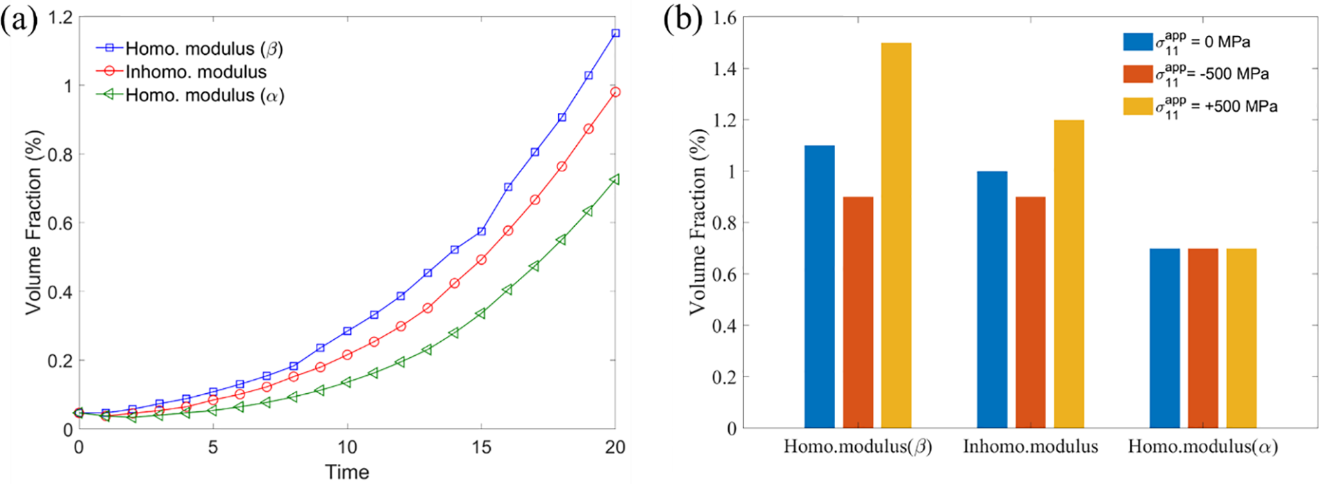
Figure 3: (a) Volume development during α precipitate growth; (b) Volume fractions of α plates at t = 20

External stresses can also alter the equilibrium shape or size of α precipitate by adding further work to the elastic strain energy. Therefore, stress along the x||[ 010 ]β direction is applied with the magnitude of σ11app=±500MPa to the simulation unit upon the growth of α. The volumes of α at t = 20 are then calculated and compared in Fig. 3b with cases where applied stresses are absent. For Case-I and Case-III, while compressive stress of 500 MPa suppresses the growth of α precipitate, tensile stresses show the opposite effect. However, the α precipitate in Case-II with homogeneous α modulus is insensitive to the applied load. The different choice of the elastic assumptions will not affect the work done by the external field. It will indeed later the elastic strain energy expressed by Eq. (5), where the elastic modulus appears directly and indirectly (involved in the ϵ¯ij through general Hooke’s law). Fig. 3 suggests that for Case-II (with homogeneous α modulus), the work performed by the current external stress with the magnitude of 500 MPa is so trivial, as compared to the elastic strain energy expressed in Eq. (5), that it is unable to promote or suppress the growth of the alpha plate. Significant change in the alpha size would be possible if a much larger stress is applied.

3.2 Stress Fields of α Precipitates

Due to the mismatch of lattice parameters of α precipitate and β matrix, stresses are concentrated at the α/β interface, which depends on the elastic moduli of two phases and the shape of α precipitates. In order to validate the accuracy of the current model, an isotropic medium is considered to contain a spherical cavity (with a modulus of zero) at the center with radius R=(1/10)l0, with l0 being the length scale. Under uniaxial loading of σzz0, the three-dimensional profile of the stress field σzznum calculated using the current model based on Eq. (4) is shown in Fig. 4a. The simulation results indicated that the stresses are concentrated at the edges of the cavity, where the modulus undergoes a sharp variation from zero to that of the isotropic media. The corresponding cross-section of the stress is shown in Fig. 4b. The calculation result is compared to the analytical solution derived by Lee et al. concerning the identical problem [31]. The relative stresses represented by the rates of σzz/σzz0 within the cross section of z=0, along x direction and away from the origin of 0.2R (the blue line in (b)) and 1.1R (the red line in (b)) are respectively present in Figs. 4c and 4d. The relative stress along the blue line increases fast when approaching the interface and suddenly decreases to zero within the cavity region. However, along the red line outside the cavity, the rate varies more smoothly and reaches a minimum of around 0.35 at the position right above the cavity. The calculation results of the developed model agree well with those of the analytical solution indicated by circles.

Figure 4: Distribution of stress component σzznum calculate by the current model within: (a) 3D simulation box; (b) 2D cross-section of z=0; (c–d) Distribution of σzz/σzz0 along the line within z=0 plane and parallel to the x-axis with a distance to the center of the spherical void of 0.2R and 1.1R, respectively

For titanium alloy with α precipitate embedded in β matrix, the evolution of stress fields of component σ11 are shown in Fig. 5 with t =1, 10 and 20. At the nucleus stage, both tension and compression stresses are observed. This stress concentration field keeps expanding along with the growth of the plane. At t = 20, the stresses are concentrated at the tips of the α plates and present certain symmetry due to the crystallography of α crystals. More specifically, stresses across the plate (along the white line in Figs. 4a–4c) are out-extracted and shown in Fig. 5d, indicating that the magnitude of stresses reaches the maximum when approaching the α/β interface, and almost keeps constant within the α plate.

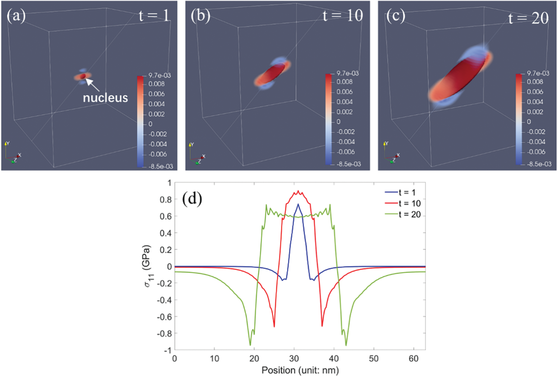
Figure 5: (a–c) Evolving stress component σ11 at the surface of α plate; (d) the stress distribution over the white line (in unit of nm) in the 3D morphology of (a–c)

However, when the homogeneous modulus assumption is applied, the stress field can be distinct from that with the inhomogeneous modulus shown above due to the variation in ΔCijkl(x) (as well as ΔSijkl(x)) and thus the elastic strain energy in Eq. (5). In Fig. 6, the stress fields of different components across the α/β interface associated with cases using α modulus or β modulus are shown and compared to the case where inhomogeneous moduli of α and β phases are strictly assigned, where σ23 and σ13 are almost zero, and therefore, only the other four components are present for comparison. For all these components, stresses using α modulus exhibit small deviations within the α phase region. Especially for σ33, the magnitude is significantly large within the α plate when β modulus is used. Matrix stresses using β modulus exhibit small deviations. All the stresses are approaching zero when moving away from the interface.

Figure 6: Stresses across the α/β interface along the direction shown in Figs. 5a–5c under different modulus assumptions

4  Conclusions

The assumption of the elastic modulus for elastically and structurally inhomogeneous solids is critical to the phase transformation process and the corresponding elastic state. The effect of modulus heterogeneity on the equilibrium shape and stress field of grown α precipitate within the β matrix during aging is systematically investigated. Three cases are considered for the calculation and comparison in this work, i.e., Case-I with a homogeneous modulus of β, Case-II with a homogeneous modulus of α, and Case-III with a heterogeneous modulus of α+β through interpolation. The main findings include:

•   The equilibrium shape (e.g., habit plane and size) of α precipitate calculated using homogeneous β modulus shows a more significant deviation from that in the heterogeneous modulus case, compared to the case where homogeneous α modulus is assumed. The size of α precipitate in Case-II with α modulus shows little dependency on the magnitude or direction of the external applied stress.

•   The local stresses across the α/β interface are calculated carefully, suggesting that stresses in Case-I show better accuracy in the β matrix, but Case-II is closer to the theoretical value within the α phase.

•   In general, for transformation from the phase of high symmetry structure to the phase of low symmetry, using elastic modulus of the low symmetry phase would give more accurate calculation results on the equilibrium morphology of the precipitate.

Acknowledgement: The authors gratefully thank Prof. Yunzhi Wang at the Ohio State University for many useful discussions on the phase transformation model for titanium alloys.

Funding Statement: DQ would like to thank the financial support from the National Key Research and Development Program of China under Grant No. 2022YFB3707803, the Key Research Project of Zhejiang Laboratory under Grant No. 2021PE0AC02, and the National Natural Science Foundation of China under Grant No. U2230102. RS acknowledges the open research fund of Songshan Lake Materials Laboratory (2021SLABFK06) and Guangdong Basic and Applied Basic Research Foundation (2024A1515011873).

Author Contributions: The authors confirm their contribution to the paper as follows: study conception and design: R. Shi; analysis and interpretation of results: D. Qiu; draft manuscript preparation: D. Qiu. All authors reviewed the results and approved the final version of the manuscript.

Availability of Data and Materials: The raw/processed data and materials required to reproduce these findings cannot be shared at this time as the data and materials also form part of an ongoing study.

Conflicts of Interest: The authors declare that they have no conflicts of interest to report regarding the present study.

References

1. Semiatin, S. L. (2020). An overview of the thermomechanical processing of α/β titanium alloys: Current status and future research opportunities. Metallurgical and Materials Transactions A, 51(6), 2593–2625. [Google Scholar]

2. Mao, H., Zeng, C., Zhang, Z., Shuai, X., Tang, S. (2023). The effect of lattice misfits on the precipitation at dislocations: Phase-field crystal simulation. Materials, 16(18), 6307. [Google Scholar] [PubMed]

3. Chen, L. Q. (2002). Phase-field models for microstructure evolution. Annual Review of Materials Research, 32(1), 113–140. [Google Scholar]

4. Eshelby, J. D. J. (1957). The determination of the elastic field of an ellipsoidal inclusion, and related problems. Proceedings of the Royal Society of London Series A: Mathematical and Physical Sciences, 241, 376–396. [Google Scholar]

5. Yanase, K., Ju, J. W. (2012). Effective elastic moduli of spherical particle reinforced composites containing imperfect interfaces. International Journal of Damage Mechanics, 21(1), 97–127. [Google Scholar]

6. Yao, Y., Chen, J., Liu, J., Chen, S. (2022). An alternative constitutive model for elastic particle-reinforced hyperelastic matrix composites with explicitly expressed Eshelby tensor. Composites Science and Technology, 221, 109343. [Google Scholar]

7. Jiang, D. (2023). Eshelby’s inclusion and inhomogeneity problem. In: Jiang, D. (Ed.Continuum micromechanics: Theory and application to multiscale tectonics, pp. 221–243. Cham: Springer International Publishing. [Google Scholar]

8. Zhao, P., Shen, C., Savage, M. F., Li, J., Niezgoda, S. R. et al. (2019). Slip transmission assisted by Shockley partials across α/β interfaces in Ti-alloys. Acta Materialia, 171, 291–305. [Google Scholar]

9. Ke, X., Wang, D., Ren, X., Wang, Y. (2020). Polarization spinodal at ferroelectric morphotropic phase boundary. Physical Review Letters, 125(12), 127602. [Google Scholar] [PubMed]

10. Zhang, T., Wang, D., Wang, Y. (2020). Novel transformation pathway and heterogeneous precipitate microstructure in Ti-alloys. Acta Materialia, 196, 409–417. [Google Scholar]

11. Qiu, D., Zhao, P., Trinkle, D. R., Wang, Y. (2020). Stress-dependent dislocation core structures leading to non-schmid behavior. Materials Research Letters, 9(3), 134–140. [Google Scholar]

12. Qiu, D., Zhao, P., Wang, Y. (2021). A general phase-field framework for predicting the structures and micromechanical properties of crystalline defects. Materials & Design, 209, 109959. [Google Scholar]

13. Moulinec, H., Suquet, P. (1998). A numerical method for computing the overall response of nonlinear composites with complex microstructure. Computer Methods in Applied Mechanics and Engineering, 157(1–2), 69–94. [Google Scholar]

14. Michel, J. C., Moulinec, H., Suquet, P. (2000). A computational method based on augmented Lagrangians and fast Fourier transforms for composites with high contrast. Computer Modeling in Engineering & Sciences, 1(2), 79–88. [Google Scholar]

15. Khachaturyan, A. G. (1983). Theory of structural transformations in solids. New York: John Wiley & Sons. [Google Scholar]

16. Shen, Y., Li, Y., Li, Z., Wan, H., Nie, P. (2009). An improvement on the three-dimensional phase-field microelasticity theory for elastically and structurally inhomogeneous solids. Scripta Materialia, 60(10), 901–904. [Google Scholar]

17. Wang, Y. U., Jin, Y. M., Cuitiño, A. M., Khachaturyan, A. G. (2001). Phase field microelasticity theory and modeling of multiple dislocation dynamics. Applied Physics Letters, 78(16), 2324–2326. [Google Scholar]

18. Wang, Y. U., Jin, Y. M., Khachaturyan, A. G. (2002). Phase field microelasticity theory and modeling of elastically and structurally inhomogeneous solid. Journal of Applied Physics, 92(3), 1351–1360. [Google Scholar]

19. Barba, D., Alabort, C., Tang, Y. T., Viscasillas, M. J., Reed, R. C. et al. (2020). On the size and orientation effect in additive manufactured Ti-6Al-4V. Materials & Design, 186, 108235. [Google Scholar]

20. Nguyen, H. D., Pramanik, A., Basak, A. K., Dong, Y., Prakash, C. et al. (2022). A critical review on additive manufacturing of Ti-6Al-4V alloy: Microstructure and mechanical properties. Journal of Materials Research and Technology, 18, 4641–4661. [Google Scholar]

21. Zhang, Y., Ma, G. R., Zhang, X. C., Li, S., Tu, S. T. (2017). Thermal oxidation of Ti-6Al-4V alloy and pure titanium under external bending strain: Experiment and modelling. Corrosion Science, 122, 61–73. [Google Scholar]

22. Liu, J., Zhang, K., Yang, Y., Wang, H., Zhu, Y. et al. (2022). Grain boundary α-phase precipitation and coarsening: Comparing laser powder bed fusion with as-cast Ti-6Al-4V. Scripta Materialia, 207, 114261. [Google Scholar]

23. Shi, R., Choudhuri, D., Kashiwar, A., Dasari, S., Wang, Y. et al. (2022). α phase growth and branching in titanium alloys. Philosophical Magazine, 102(5), 389–412. [Google Scholar]

24. Shi, R., Wang, Y. (2013). Variant selection during α precipitation in Ti-6Al–4V under the influence of local stress—A simulation study. Acta Materialia, 61(16), 6006–6024. [Google Scholar]

25. Cahn, J. W., Hilliard, J. E. (1958). Free energy of a nonuniform system. I. Interfacial free energy. The Journal of Chemical Physics, 28(2), 258–267. [Google Scholar]

26. Zhang, F., Chen, S. L., Chang, Y., Ma, N., Wang (2007). Development of thermodynamic description of a pseudo-ternary system for multicomponent Ti64 alloy. Journal of Phase Equilibria and Diffusion, 28, 115–120. [Google Scholar]

27. Steinbach, I., Pezzolla, F., Nestler, B., Seeßelberg, M., Prieler, R. et al. (1996). A phase field concept for multiphase systems. Physica D: Nonlinear Phenomena, 94(3), 135–147. [Google Scholar]

28. Burgers, W. G. (1934). On the process of transition of the cubic-body-centered modification into the hexagonal-close-packed modification of zirconium. Physica, 1(7), 561–586. [Google Scholar]

29. Ledbetter, H., Ogi, H., Kai, S., Kim, S., Hirao, M. (2004). Elastic constants of body-centered-cubic titanium monocrystals. Journal of Applied Physics, 95(9), 4642–4644. [Google Scholar]

30. Mills, M., Hou, D., Suri, S., Viswanathan, G. (1997). Orientation relationship and structure of alpha/beta interfaces in conventional titanium alloys. Boundaries & Interfaces in Materials: The David A. Smith Symposium, pp. 295–301. [Google Scholar]

31. Lee, H. K., Ju, J. W. (2007). A three-dimensional stress analysis of a Penny-shaped crack interacting with a spherical inclusion. International Journal of Damage Mechanics, 16(3), 331–359. [Google Scholar]