Data-Driven Structural Topology Optimization Method Using Conditional Wasserstein Generative Adversarial Networks with Gradient Penalty

1  Introduction

The study of topology optimization has received significant attention since Bendsoe and Kikuchi’s pioneering work. Several topology optimization methods have been proposed, including the Solid Isotropic Material with Penalization method, the Level Set method, the Evolutionary Structural Optimization method, the moving morphable components method and the independent continuous mapping method [1–5]. These methods have been applied successfully to a wide range of physical optimization problems, investigating structural, acoustic, electromagnetic, or optic performances.

In the field of topology optimization, a primary objective is to improve computational efficiency. However, traditional topology optimization methods suffer from an inherent drawback known as “the curse of dimensionality”. As the number of design variables and iteration steps increase, the computational cost grows exponentially. Despite recent advancements in topology optimization, cumbersome iterations and finite element calculations still cannot be circumvented. Consequently, real-time topology optimization remains an open problem.

In recent years, data-driven topology optimization methods have emerged as a research hotspot. Current works for topology optimization using machine learning can be broadly categorized into two groups depending on whether they are combined with finite element analysis (FEA). The first approach involves initially obtaining a rough solution through a limited number of FEA iterations, which is then used as input for a machine learning model to obtain a more accurate topology optimization structure. This approach has been explored in several studies [6–8]. Another approach is the deep learning-based noniterative topology optimization method, where initial conditions and design variables directly serve as inputs to a machine learning model for predicting the topology optimization outcomes. Commonly used machine learning models comprise Convolutional Neural Networks, Generative Adversarial Networks (GAN), and U-Net [9–13]. This approach requires a labeled training dataset and the construction and training of a corresponding neural network model, which is then used to predict optimal configurations for cases within the same distribution as the training set. Common methods for dataset generation involve employing conventional topology optimization algorithms such as SIMP and density-based approach; however, some researchers have utilized models like Wasserstein Generative Adversarial Nets (WGAN) and Variational Autoencoder to produce the requisite topology optimization dataset for training [14–16]. For instance, Lei et al. combined the Moving Morphable Components method with machine learning, enhancing the speed and flexibility of real-time topology optimization [17]. Wang et al. introduced a data-driven structural design optimization approach utilizing isogeometric analysis, which fully leverages the advantages of NURBS to achieve more accurate and computationally efficient design solutions [18]. Yin et al. applied the physical information neural network to the field of topology optimization, establishing two neural networks to replace expensive ones by utilizing the similarity of pseudo-density fields [19]. Rawat et al. proposed a topology optimization method based on conditional Wasserstein generative adversarial networks, achieving structures similar to traditional methods but with lower computational costs [9]. Rade et al. introduced a deep learning framework for three-dimensional topology optimization, aligning closely with traditional algorithms while emphasizing high-resolution capabilities [20]. Xiang et al. proposed a deep convolutional neural network for 3D structural topology optimization while predicting structures close to optimal in a short time, achieving a significant reduction in computational costs [21]. Greminger used a generative adversarial network to create a generalized topology optimization method with manufacturability constraints, broadening the applicability of optimization techniques [22].

In this paper, we proposed a data-driven structural topology optimization method by developing a Conditional Wasserstein Generative Adversarial Network with Gradient Penalty (CWGAN-GP). The dataset is generated by the FEM-based based SIMP method which includes over 20,000 samples. Then, we set up a conditional Wasserstein generative adversarial network. Then, we train this network using the dataset. The trained network receives the boundary and load conditions as the encoded constraint conditions, and outputs the optimized structure. For given boundary and load conditions, the network can obtain a unique optimization structure one-to-one. We also apply Pix2pixGAN to optimize the boundary of the generated structures using CWGAN-GP. Compared with the structure obtained by CWGAN-GP, Pix2pixGAN can enhance the clarity of the structure significantly.

2  Conditional Wasserstein Generative Adversarial Networks with Gradient Penalty (CWGAN-GP)

2.1 Generative Adversarial Networks

The Generative Adversarial Network consists of a generator G and a discriminator D. The generator G creates structures Gz by inputting random noise, aiming to generate structures that satisfy the real sample distribution as much as possible. The generated image is then inputted to the discriminator D, which determines whether the input data is from the real data set or from generated data D. If it is determined to be real, D outputs 1; otherwise, D outputs 0. The loss function of traditional GAN is defined as follows:

minGmaxDV(D, G)=Ex∼Pdata (x)[log⁡D(x)]+Ez∼Pz(z)[log⁡(1−D(G(z)))](1)

where x represents a true sample, Pdata(x) represents the real sample distribution, z is a random noise, and Pz(z) represents the sample distribution of the noise. D(G(z)) indicates the probability of the sample generated by G(Z) ultimately being judged as true or false by the discriminator D. The purpose of GAN is to generate samples that are closer to real samples, with D(G(Z)) approaching 1. This is achieved by minimizing the value of V(D,G). For the discriminator D, the aim is to get D(G(Z)) closer to 0 and make the real sample D(X) closer to 1, in order to maximize the value of V(D,G).

Traditional deep learning methods typically require a large number of training samples to effectively handle complex image and sample distributions. In contrast, Generative Adversarial Networks are able to generate samples with similar precision using fewer training samples compared to deep convolutional neural networks. Despite these advantages, traditional GANs encounter challenges when dealing with constrained problems because the input data is typically in the form of noise, rather than pre-defined constrained data. This can make it difficult to ensure that the generated samples satisfy specific constraints or specifications. Another challenge with traditional GANs is the optimization of the generator’s objective function. This function is equivalent to solving the Jensen-Shannon (JS) divergence under the optimal discriminant, which presents difficulties in effectively optimizing the generator. Consequently, alternative approaches, such as Wasserstein GANs and Least Squares GANs, have been proposed to address this issue and improve the stability of GAN training.

2.2 Conditional Generative Adversarial Networks and Pix2pix

In order to overcome the limitation that the generator G cannot handle conditional constrained data, researchers proposed the use of Conditional Generative Adversarial Networks (CGANs) [23]. This involves adding conditional labels to both the generator and the discriminator. Specifically, the input to the generator consists of both noise labels and constrained labels, which are combined and used to generate the corresponding output G(z∣y). The objective functions of CGANs are as follows:

The objective function of CGAN is:

minGmaxDV(D,G)=Ex∼Pdata (x)[log⁡D(x∣y)]+Ez∼Pz(z)[log⁡(1−D(G(z∣y)))](2)

By making modifications to the conventional GAN loss function, it becomes possible to impose constraints on the data generation process, taking into account both the distribution of the constrained condition y and the noise z. This modification ensures that the generated samples conform to specific constraints, eliminating the randomness of the output.

Pix2pix is a variant of CGAN, where the generator G only receives the conditioning input y, rather than a noise input z. On the other hand, the discriminator D can process both the conditioning and noise inputs. In Pix2pix, the GAN loss is augmented with the L1 distance metric, which serves to mitigate image blurring [24].

The L1 loss function is:

LL1(G)=Ex, y, z[‖y−G(x, z)‖1](3)

The loss function of Pix2pix is:

G∗=arg⁡minGmaxDLcGAN(G, D)+λLL1(G)(4)

2.3 GAN Based on Wasserstein Distance and Gradient Patiently (WGAN-GP)

The generator in the original GAN usually uses JS divergence or KL divergence, but if the generated sample distribution does not coincide with the original sample distribution, the gradient will easily disappear. Martin et al. replaced JS or KL divergence with Wasserstein distance, which can ensure that even if the two distributions do not overlap, Wasserstein distance can still reflect their distance, avoiding the problem that the generator cannot be trained [25,26].

Wasserstein distance is defined as follows:

W(Pr, Pg)=infγ∼Π(Pr, Pg)E(x, y)∼γ[‖x−y‖](5)

where Pr is the distribution of true data and Pg is the distribution of generated data, Π(Pr, Pg) is the set of all possible distributions by combining Pr and Pg.

For each possible distribution, we withdraw the samples x and y, calculate the expectation distance E(x, y)∼γ[‖x−y‖. Then in all possible distributions, we stipulate that the infimum of the expected value infγ∼Π(Pr, Pg) is Wasserstein distance. As it is difficult to solve infγ∼Π(Pr, Pg), we change it into:

W(Pr, Pg)=1Ksup‖f‖L≤KEx∼Pr[f(x)]−Ex∼Pg[f(x)](6)

A Lipschitz function is characterized by the property that the difference in its output values is bounded by a constant multiple of the difference in its input values. Based on the Lipschitz function continuity, the upper formula can be turned into an approximate solution to the following equation:

K⋅W(Pr, Pg)≈maxw:‖fw‖L≤KEx∼Pr[fw(x)]−Ex∼Pg[fw(x)](7)

where fw(x) is a discriminator network with parameter w. K is the Lipschitz constant of the discriminator. The Lp-parameter of fw(x) gradient is not greater than K, ‖f‖L≤K.

According to the aforementioned loss function, the generator and the discriminator will be alternately trained, aiming to minimize the Wasserstein distance to narrow the distribution between the real sample space and the generated sample space.

For WGAN, the weighted parameter values of fw(x) are limited in a certain range [−c, c] (in this paper, the interval is [−0.01, 0.01]). In doing so, the derivative value during the derivative calculation process will not exceed a certain range and the Lipschitz continuity condition will be satisfied. But in the training process, the discriminator D hopes to be able to distinguish between true and false samples as much as possible, and the weight parameter w will limit the range of the parameter values of each network, then in this case, the optimal strategy will make all parameter values go to extremes. After verification, we found that the network parameters of the discriminator D are usually distributed in the two extremes of the maximum and minimum. In addition, weight clipping will cause the gradient to disappear or explode. The reason is that after the two poles of the parameter are stacked if the clipping threshold value is small, the gradient will attenuate after multiple layers. If its value is large, the gradient solution after multiple layers will explode.

This issue primarily arises from the Lipschitz constraint. During the training of the discriminator, the gradient norms tend to converge around a value K. To address this issue, we introduce a gradient penalty function given by:

L=[‖∇xD(x)‖p−K]2(8)

With K = 1 and the introduction of the weight parameter λ, the loss function for the WGAN-GP network is formulated as follows:

L(D)=−Ex∼Pt[D(x)]+Ex∼Pg[D(x)]+λEx∼Px[(‖∇xD(x)‖p−1)2](9)

where x^=εxr+(1−ε)xg.

The utilization of Wasserstein distance with gradient penalty as the loss function in WGAN mitigates the issue of binary polarization and facilitates model training, thereby contributing to its overall effectiveness.

3  Topology Optimization Using CWGAN-GP

3.1 Dataset

The dataset is generated using the SIMP topology optimization algorithm. In this case, we take the surface force and Dirichlet boundary conditions as design variables. What’s more, the surface force includes concentrated force and distributed force. The range of surface force is [0–1000], and the Dirichlet boundary conditions randomly change. By taking different design variables, we obtained 16,525 topology optimization structures. As shown in Fig. 1, the left figure illustrates the force conditions (blue bar) and Dirichlet boundary conditions (red bar), and the right figure depicts the topology structure obtained by the SIMP algorithm [27,28]. Dirichlet boundary conditions are applied at the domain’s boundaries, while the forces are represented by blue rectangles, indicating both the magnitude and direction of the applied loads.

Figure 1: Force/Boundary conditions and corresponding topology optimization structure

Before using the dataset to train the CWGAN-GP model, we need to encode the design variables to form 16,525 pairs of topology optimization structures. The coding rules are as follows, since every design variable acts in two directions, the x and y, so we set a one-dimensional channel for every design variable in every direction. In this case, the one-dimensional channels include two force channels fx, fy, and two Dirichlet boundary channels bx, by.

As shown in Fig. 2, the node number of the finite element mesh in this case is 80 × 80. Each mesh can be looked upon as a pixel and the number of the pixels on the four boundaries is 79×4. So, the length of each channel is 316. As there are four channels, the length of encoded design variables is 316×4.

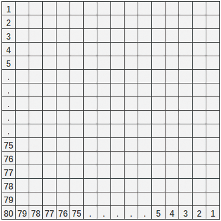
Figure 2: Schematic diagram of finite element mesh nodes

3.2 Network Structure of CWGAN-GP for Topology Optimization

Fig. 3 shows the structure of the generative network G. Inspired by Pix2pixGAN, the initial random noise vector z is abandoned. The encoded design variables mentioned above are used as the initial input label of the generative network G. Firstly, we design a fully connected layer FC and dropout layer to covert the label x into a vector with the dimension 5×5×8×D. The D mentioned in the figure refers to the depth of the deconvolution operation, which can be adjusted according to the memory size of the GPU. Secondly, we designed four deconvolution layers to map the data from a one-dimensional vector to a two-dimensional topology optimization structure. What’s more, in order to avoid zero gradients, we abandon the pooling layer that usually follows the deconvolution layer. We choose ReLU as the activation function. The output of the generator G is a matrix with a dimension of [80, 80, 1], which is the two-dimensional fake topology optimized structure.

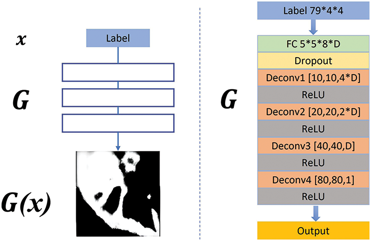
Figure 3: The structure of the generative network G

Fig. 4 shows the structure of the discriminator network D. The input of D is the combination of design variables and fake/real topology-optimized structure. As the size of the unfolded topology optimized structure matrix is 1×6400, the size of encoded design variables is 1×1264, those could be merged into a vector of 1×7664. In order to facilitate the convolution operation, we need to reshape the merged vector into a square matrix. However, the square of 7664 is not an integer, so we introduce a zero-padding strategy which needs to pad zero after the merged vector. In this case, we extended the merged vector to 1×7744, which could be reconstructed into a matrix with dimensions [88, 88, 1], by the zero-padding strategy. We design four convolution layers for the discriminator D, which could map the data from merged vectors to high-dimensional information to low-dimensional features. We choose LReLU as an activation function, the parameter value of LReLU is 0.2 [29]. The output of the discriminator D is the number of 1/0, which corresponds to real and fake, respectively.

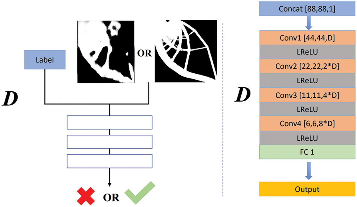
Figure 4: The structure of the discriminator network D

3.3 Pseudo Code

The flowchart of CWGAN-GP algorithm is as Algorithm 1.

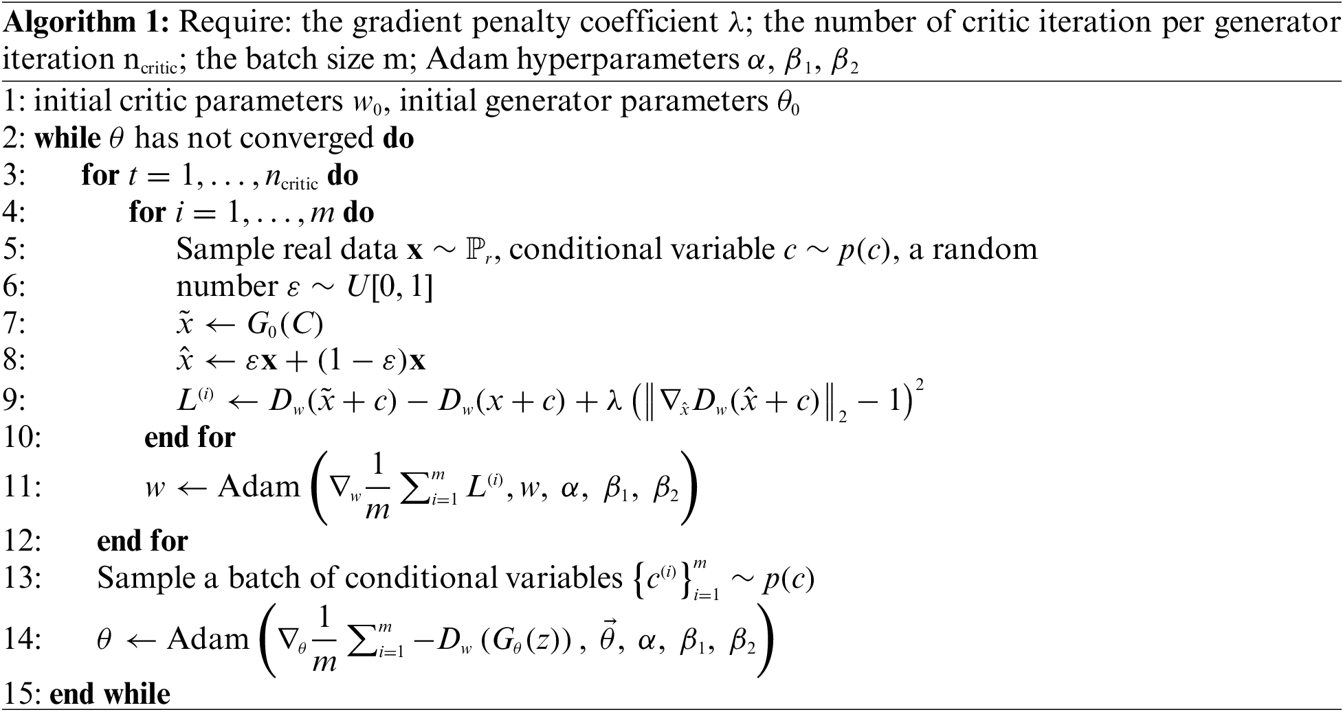
Traditional GAN will introduce noising z, in this paper, the noising z is abandoned and only the condition c is input into G. The discriminator D is trained one time and corresponding, the generator G is trained four times. In Step 5, the generator G generates faked data x. As shown in the following equation, the sum of x and c is equivalent to the weighted sum of real data εx and generated data (1−ε)x.

x+c←ε(x+c)+(1−ε)(x+c)=εx+(1−ε)x+c(10)

4  Enhancing the Clearance of Topology Structures Using Pix2pixGAN

Compared with the structures generated by SIMP, a few structures generated by CWGAN-GP are not accurate. For example, some complex topology optimization structures have many subtle structures, which are difficult to generate accurately based on the CWGAN-GP alone. In order to solve the problem of low precision in complex structures, the image enhancement method based on Pix2pixGAN is developed.

Fig. 5 illustrates the structure of Pix2pixGAN. The Pix2pixGAN takes the complex topology optimization structure generated by CWGAN-GP as the input of generator G. Firstly, the generator outputs the G(x) as a fake complex structure. Then, the complex topology optimization structure generated by CWGAN-GP is merged with the G(x) or the structure generated by SIMP to as the input of discriminator D. In this paper, we adopted the U-Net network structure in generator G and adopted the PatchGAN in discriminator D, in which the receptive field is set as 70×70 [30]. The complete methodology proposed in this paper is illustrated in Fig. 6 for a comprehensive understanding.

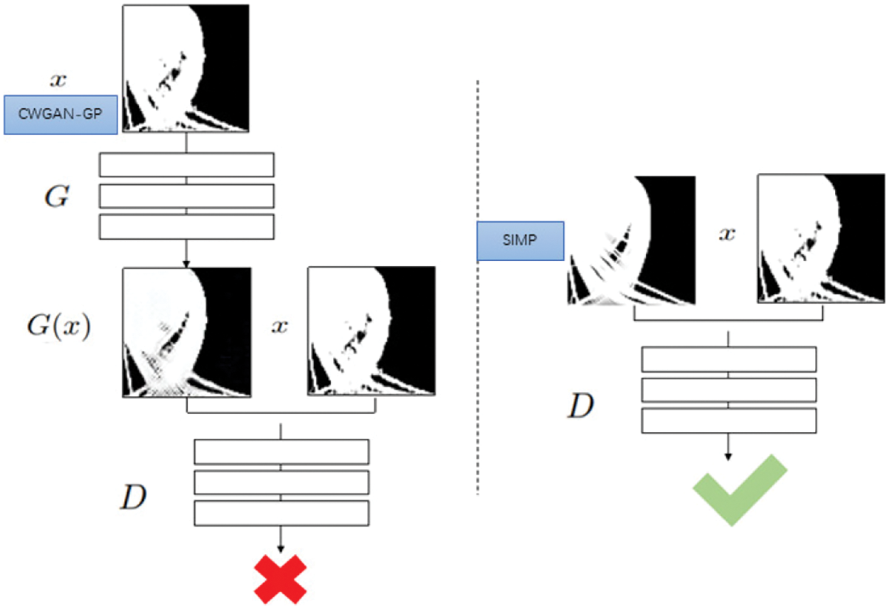
Figure 5: Pix2pix model structure

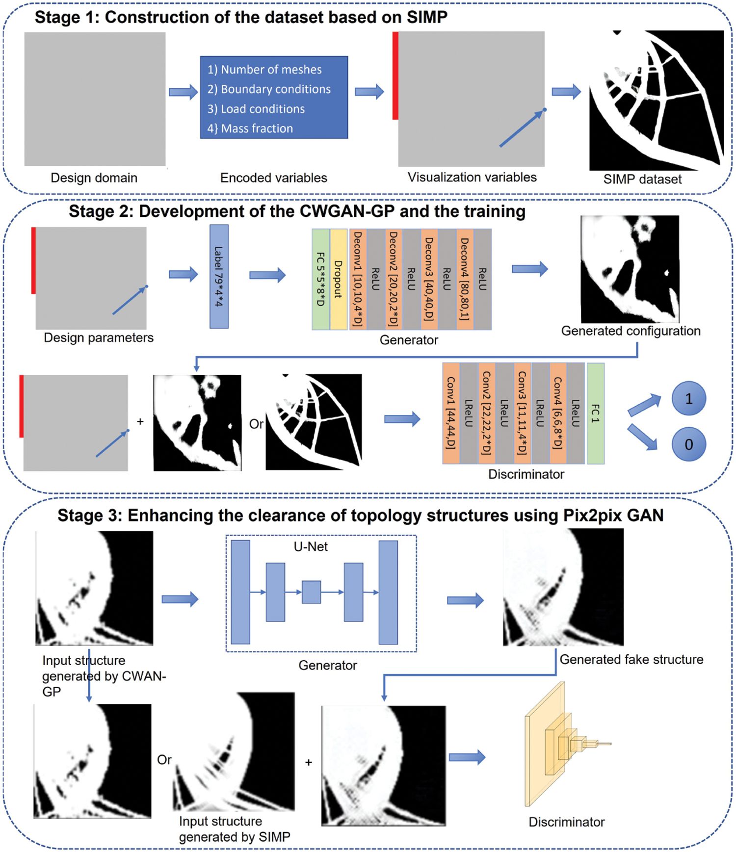
Figure 6: Process of CWGAN-GP and Pix2pixGAN

5  Numerical Examples

5.1 Real-Time Topology Optimization Using CWGAN-GP

There are 16,525 pairs of topology optimization structures in the dataset, and the sample ratio between the training set and the testing set is 0.89:0.11, namely 14,708 samples are used for training and 1817 samples are used for testing. We choose the ADAM optimizer to train CGWAN-GP and the number of iterations is set to 150. The experiment is based on NVIDIA RTX2080Ti GPU, Tensorflow platform, and Python3.

The trained CWGAN-GP model is verified by the testing set. Table 1 shows some high-quality topology structures generated by CWGAN-GP and the comparison with SIMP. To quantitatively illustrate structural similarity and verify the effectiveness of CWGAN-GP, two evaluation indicators for evaluating image quality are employed: one is Peak Signal to Noise Ratio (PSNR), another one is Structural Similarity Index Measure (SSIM) [31,32]. The PSNR and SSIM values are calculated every 10 iteration steps by testing set. As shown in Figs. 7 and 8, after 100 iterations, the curve is relatively stable and the algorithm tends to converge. As shown in Table 2, for the testing set data, the maximum value of SSIM is 0.847, and the maximum value of PSNR is 19.64 dB. The above experimental results prove that the CWGAN-GP algorithm can effectively generate topology optimization structures. However, when CWGAN-GP faces complex structures, the results will be fuzzy. We hope to obtain accurate complex topology optimization structures through CWGAN-GP, so the next work is to improve the precision of complex topology optimization structures.

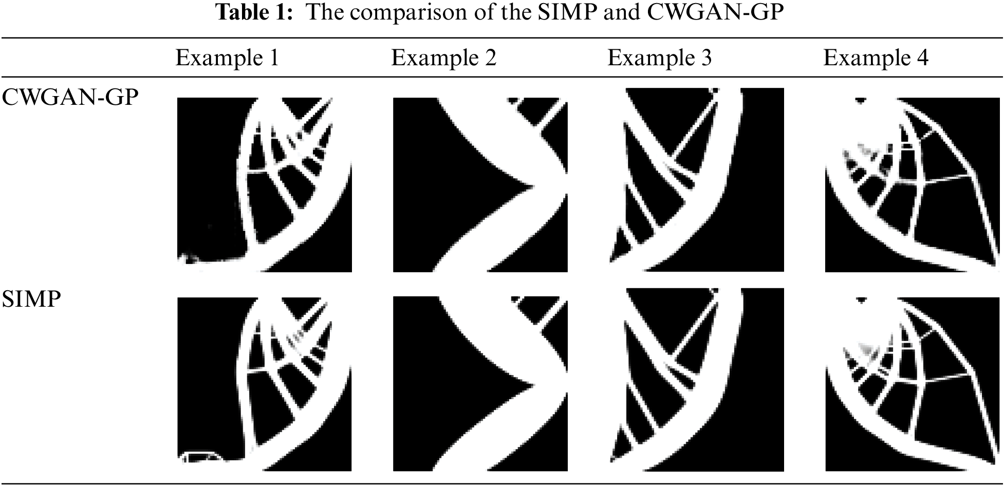
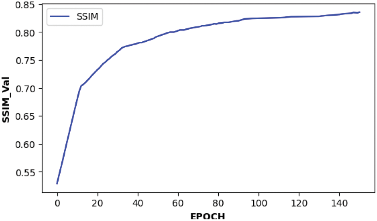
Figure 7: Structural similarity SSIM with iteration number curve

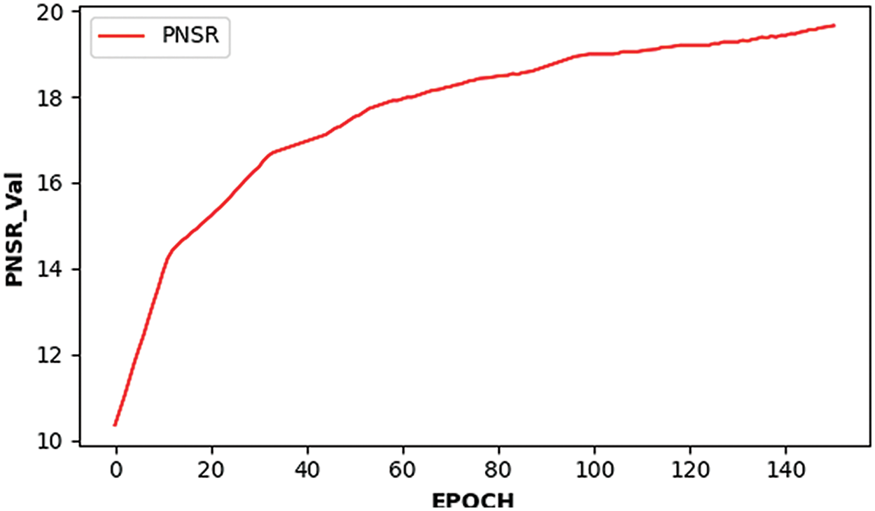
Figure 8: The maximum peak signal-to-noise ratio PSNR varies with the number of iterations

5.2 Transfer Learning Using Pix2pix Based on CWGAN-GP

As shown in Table 3, some complex structures generated by CWGAN-GP have low precision. Two reasons cause this result. The first is the uneven distribution of samples in the training dataset, as the number of samples with complex structures is small, which makes the model can’t fully learn its structural features. The second is that there are too many details features in some complex structures, and the generator sometimes can not effectively reflect these details features, resulting in fuzzy results.

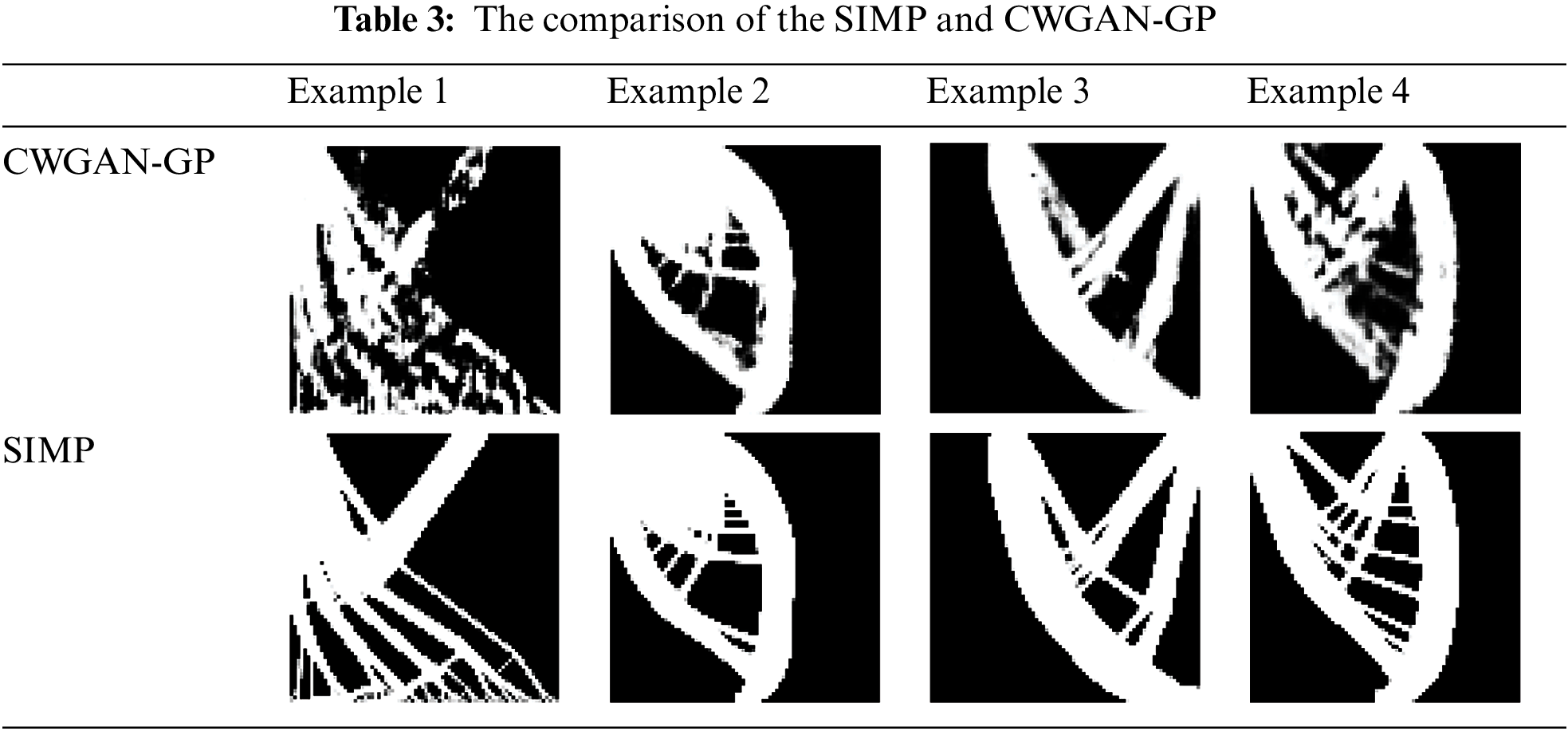
We use the Pix2pix model to further improve the precision of the complex topology optimization structures generated by CWGAN-GP. Based on the previous work, we prepared about 1800 pairs of experimental data for training Pix2pix model. The input and output are grayscale pictures with size 80×80 and pixel value range (0, 1).

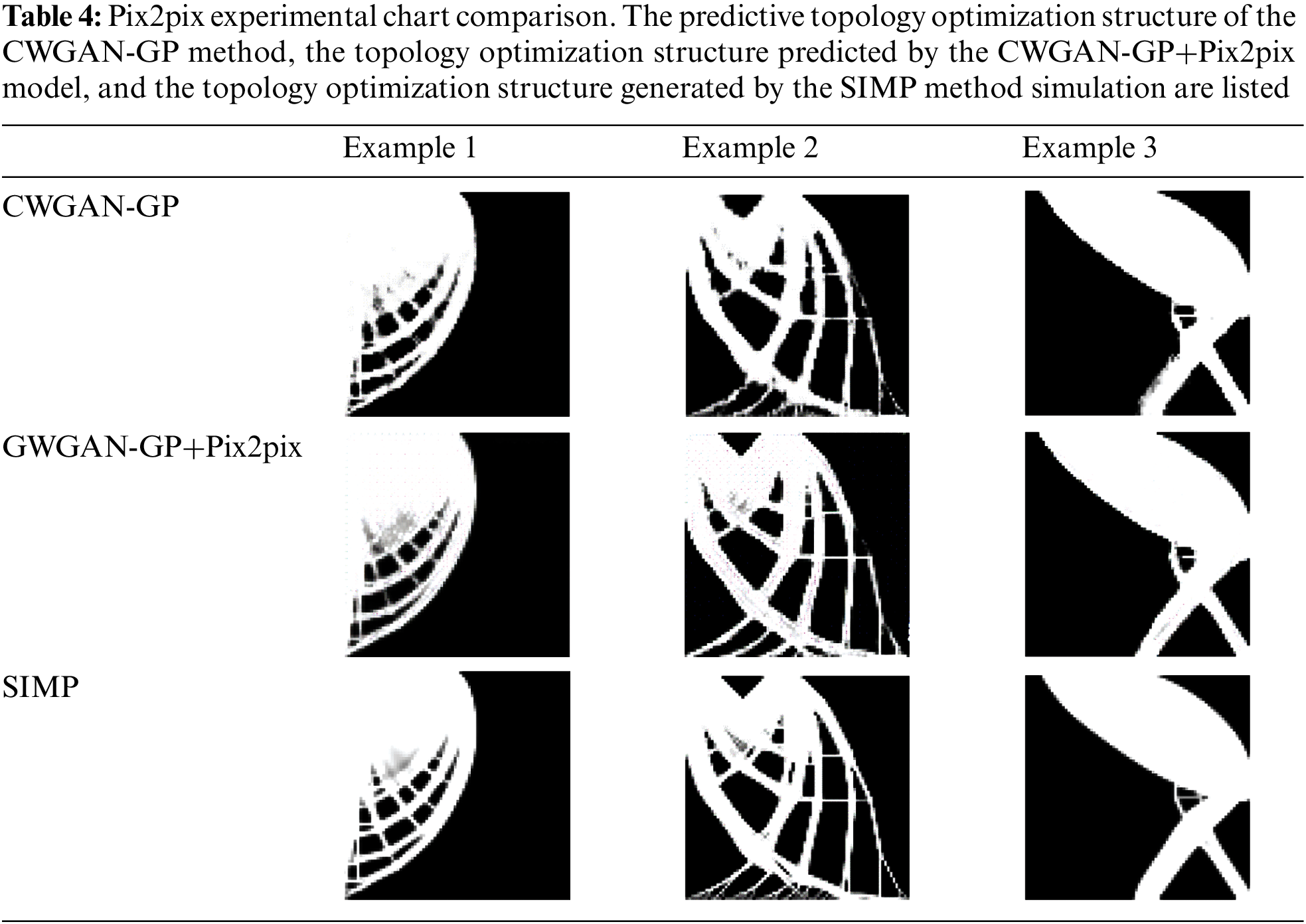
The experiment is carried out on the grayscale pictures dataset obtained by CWGAN-GP and SIMP methods. The ratio of the training set to the testing set is 0.7:0.3, there are about 500 samples in the testing set. The experiment is based on NVIDIA RTX2080Ti GPU, Tensorflow platform, and Python3. We use the ADAM optimizer to train the model, the learning rate is set to 0.0002, the value of the first momentum parameter is set to 0.5, the batch size value is set to 1, the 1-norm loss function weight is set to 100, the iterations is set to 200. The trained CWGAN-GP model is verified by the testing set. The comparison of results is shown in Table 4, compared with single CWGAN-GP, the combination of CWGAN-GP and Pix2pix eliminates fuzzy phenomenon effectively.

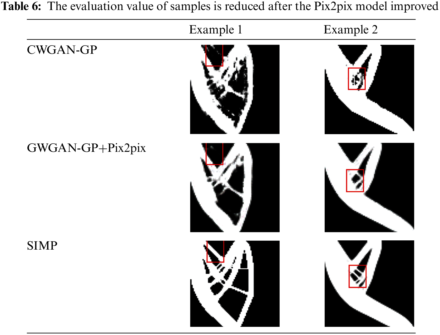
To quantitatively illustrate the improvement of results, we calculate the PSNR and SSIM values of the single CWGAN-GP model and the combined model on the testing set. However, although the combination of Pix2pix improves the precision, the accuracy of some structures decreases, and we cannot quantify this impact at present. Table 5 shows that the max values of SSIM and PSNR are 0.85 and 19.8 dB, which are lower than the corresponding values of 0.87 and 20.14 dB obtained by CWGAN-GP. However, the values of SIMP and PSNR are decreased, as shown in Table 6, topology optimization structures become clearer than those obtained by CWGAN-GP. The reason for this phenomenon is that some of the pictures processed by Pix2pix have some subtle structures deleted by mistake, which is hard to control.

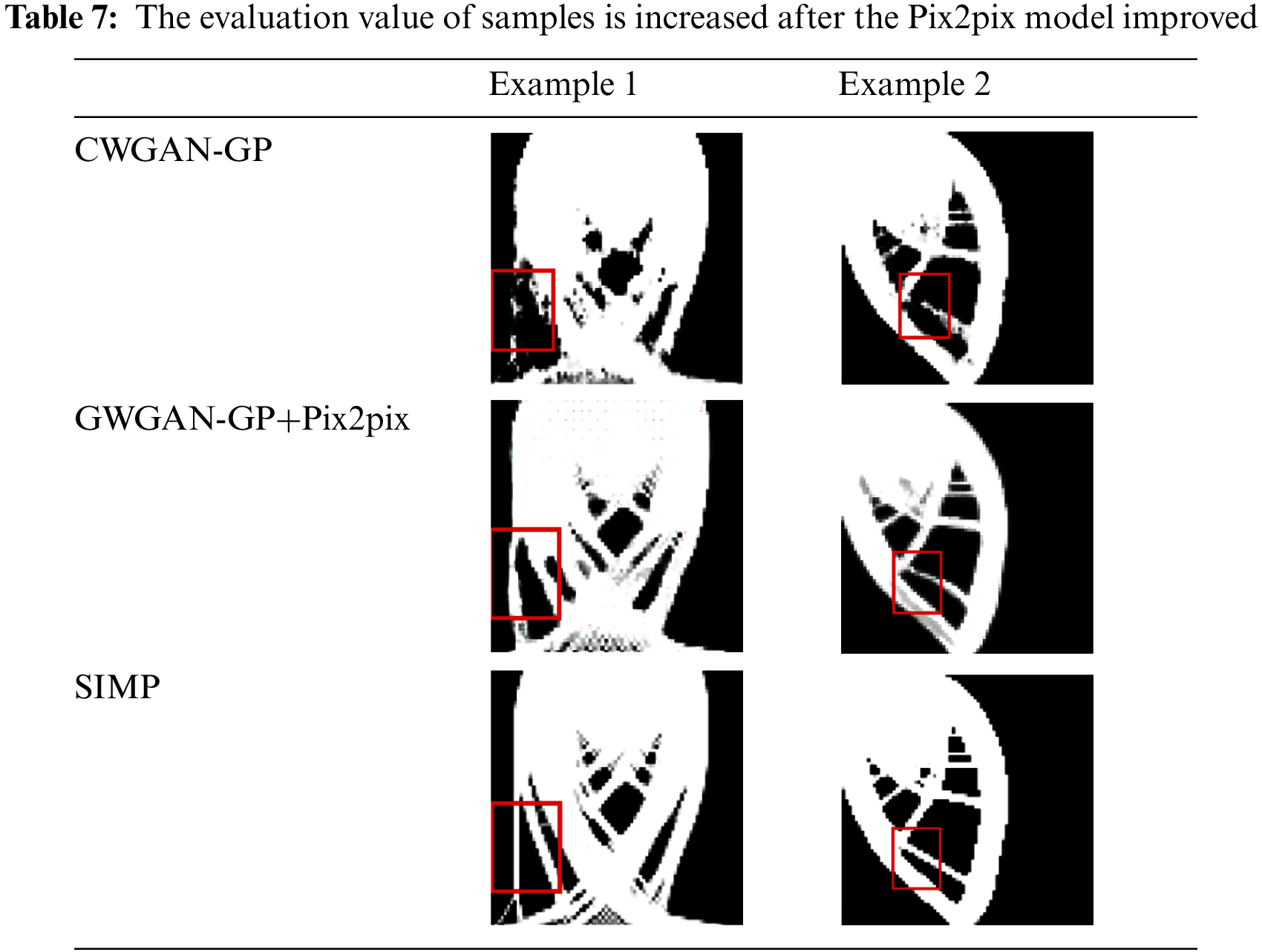
In this experiment, we also found that the values of PNSR and SSIM do not always go low. Sometimes, the values increase and the topology structures are approaching the true structures obtained by the SIMP method. Table 7 compares another group of structures generated by CWGAN-GP, CWGAN-GP+Pix2pix and SIMP method, which significantly improved accuracy by Pix2pix.

To further evaluate the effectiveness of the Pix2pix method, as shown in Figs. 9 and 10, we randomly select 0–100 samples on the testing set to compare the values of PSNR and SSIM by CWGAN-GP and CWGAN-GP+Pix2pix, respectively. The red curves are the interpolated curves by CWGAN-GP+Pix2pix and the blue dotted curves are generated by CWGAN-GP. There is little difference between the two curves in each figure. Considering all aspects, after the process of Pix2pix, although the evaluation value sometimes decreases, we actually get more accurate topology optimization structures.

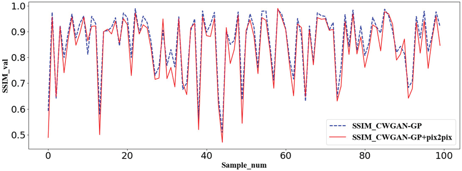
Figure 9: Structural similarity curves of CWGAN-GP and CWGAN-GP+Pix2pix models

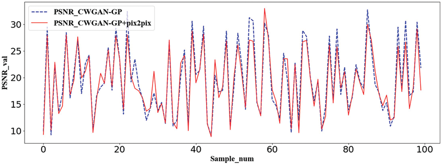
Figure 10: Peak signal to noise ratio curves of CWGAN-GP and CWGAN-GP+Pix2pix models

5.3 3D Real-Time Topology Optimization Using CWGAN-GP

The CWGAN-GP method proposed above can also be applied to the topology optimization of three-dimensional structures. This section gives the following cases: using the CWGAN-GP method to predict the structural topology optimization of a 3D design domain with a size of 4×20×60. In this design domain, the displacement boundary conditions are fixed, and the design variables are the number of loads, the position of the load, and the volume retention rate. We have obtained a total of 391 topology optimization samples under this working condition by 3D SIMP algorithm [33]. The ratio of the training set to the testing set is 0.9:0.1, that is, 352 pairs of samples are used for training and 39 pairs of samples are used for testing. The result of structural topology optimization is represented by the unit material density value with a value range of [0, 1].

The design variables can be looked upon as a one-dimensional channel which consists of two parts: displacement/load variables and volume retention fraction condition. The specific condition rules are as follows:

(1) Displacement/load variables: Only consider the surface where with constraints or force load, set the value of the node with displacement boundary constraint to 1, set the value of the node with load to 10, and set the other free nodes values to 0. If the design variables include the load size, we can also set the value of the load node to the actual size.

(2) Volume retention fraction variables: A one-dimensional vector with a length of 20 is set. In order to effectively identify the characteristics of different volume retention scores, the node value of the vector is set to ten times the actual volume retention score.

In this case, the load condition is located on the upper surface of the beam, and the displacement constraint is located on the lower surface of the beam. The other surfaces have no boundary conditions, so only the upper and lower surfaces be coded. In this experiment, the size of the upper and lower surfaces is 4×60, so the conditions size of the displacement/load conditions part is 2×4×60; the conditions size of the volume retention rate conditions part is 1×20, and the two parts are expanded and spliced to form a total length. It is a 1×500 conditions vector.

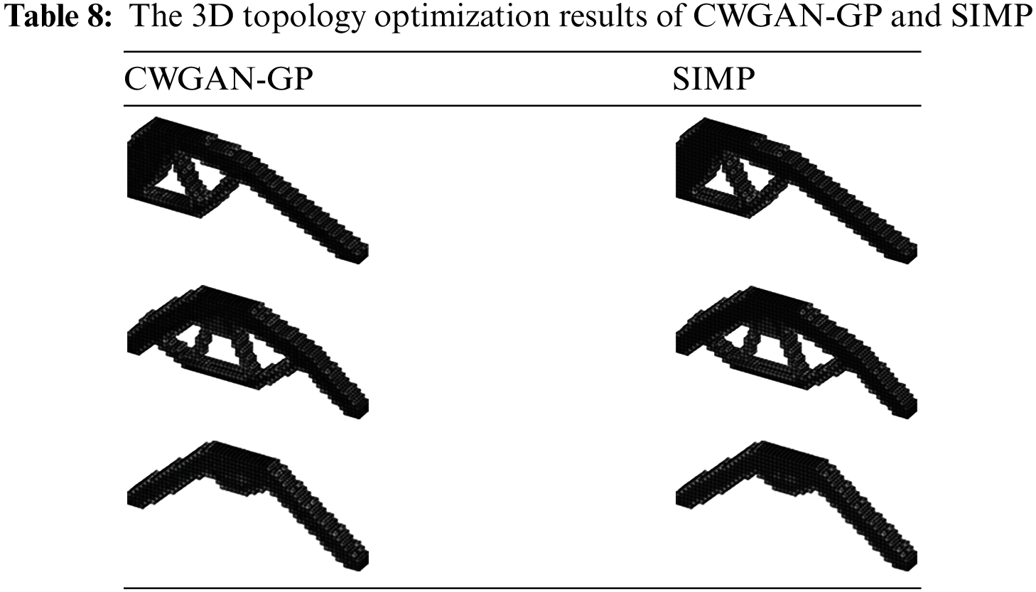
This case uses the same model network structure as above, we only adjust the input and output sizes of each layer network in the generator and discriminator for the design domain and conditions vector size and use the same training method as above to train the three-dimensional case. The prediction results of part of the test set are shown in Table 8. The experiment results prove that CWGAN-GP shows potential for real-time topology optimization of certain 3D structures. However, further data and additional experiments are necessary to demonstrate its full generalization capabilities.

6  Conclusion

We proposed a real-time structural topology optimization method using Conditional Generative Adversarial Networks with Gradient Penalty. The dataset is generated by the SIMP topology optimization algorithm. The first part of the work uses the denoising CWGAN-GP method, removes the noise, combines CGAN and WGAN’s improved version of WGAN-GP, generates a topology optimization structure corresponding to the constraint conditions, and uses the evaluation criteria of SSIM and PSNR. Preliminary evaluation proves the feasibility of this method in the field of topology optimization. In the second part of the work, the Pix2pix method is used to remove the blur, and a clearer image is generated, a better structure pattern is obtained. Some complex structures can also be better predicted. Judging from the pictures synthesized at the end of the two works, our experimental method compared with the real structure, the peak signal-to-noise ratio reached 19.79 dB, and the structural similarity reached 0.85. It is also worth mentioning that the total time taken to make predictions for the two models using the research methodology employed in this paper is approximately 1 s, which is a significant improvement in time efficiency compared to the 1800 s of computation time consumed by the traditional SIMP method. In addition, this paper also tries to apply the CWGAN-GP algorithm to the three-dimensional structure and obtains accurate topology optimization results. What’s more, the CWGAN-GP can be applied to both 2D structures and 3D structures. The above experimental results show that the algorithm in this paper can better realize real-time topology optimization, and provides a reference idea for deep learning and generative adversarial networks in the field of topology optimization or mechanics.

However, the method proposed in this article still has limitations. For example, the trained model can only be applied to the design domain of the same size, and the encoding rules of design variables are not generic. In the future, we will further develop more versatile real-time methods to handle topology optimization tasks under other complex conditions.

Acknowledgement: The authors would like to thank the anonymous reviewers and the editors of the journal. Your constructive comments have improved the quality of this paper.

Funding Statement: This work is supported by the National Key Research and Development Projects (Grant Nos. 2021YFB3300601, 2021YFB3300603, 2021YFB3300604) and Fundamental Research Funds for the Central Universities (No. DUT22QN241).

Author Contributions: The authors confirm contribution to the paper as follows: study conception and design: Xiaochen Liu, Qingrong Zeng, Xuefeng Zhu; data collection: Xiangkui Zhang, Ping Hu; analysis and interpretation of results: Xiaochen Liu; draft manuscript preparation: Qingrong Zeng. All authors reviewed the results and approved the final version of the manuscript.

Availability of Data and Materials: The datasets generated during and/or analyzed during the current study are available from the corresponding author on reasonable request.

Ethics Approval: Not applicable.

Conflicts of Interest: The authors declare that they have no conflicts of interest to report regarding the present study.

References

1. de Gournay F. Velocity extension for the level-set method and multiple eigenvalues in shape optimization. SIAM J Control Optim. 2006;45(1):343–67. doi:10.1137/050624108. [Google Scholar] [CrossRef]

2. Xie Y, Steven G. A simple evolutionary procedure for structural optimization. Comput Struct. 1993;49(5):885–96. doi:10.1016/0045-7949(93)90035-C. [Google Scholar] [CrossRef]

3. Zhang W, Yuan J, Zhang J, Guo X. A new topology optimization approach based on moving morphable components (MMC) and the ersatz material model. Struct Multidiscipl Optim. 2015;53:1243–60. doi:10.1007/s00158-015-1372-3. [Google Scholar] [CrossRef]

4. Jiang X, Liu C, Du Z, Huo W, Zhang X, Liu F. A unified framework for explicit layout/topology optimization of thin-walled structures based on moving morphable components (MMC) method and adaptive ground structure approach. Comput Methods Appl Mech Eng. 2022;396:115047. doi:10.1016/j.cma.2022.115047. [Google Scholar] [CrossRef]

5. Wang W, Ye H, Sui Y. Lightweight topology optimization with buckling and frequency constraints using the independent continuous mapping method. Acta Mech Solida Sin. 2019;32:310–25. doi:10.1007/s10338-019-00088-5. [Google Scholar] [CrossRef]

6. Lin Q, Hong J, Liu Z, Li B, Wang J. Investigation into the topology optimization for conductive heat transfer based on deep learning approach. Int Commun Heat Mass Transf. 2018;97:103–9. doi:10.1016/j.icheatmasstransfer.2018.07.001. [Google Scholar] [CrossRef]

7. Jiang X, Wang H, Li Y, Mo K. Machine learning based parameter tuning strategy for MMC based topology optimization. Adv Eng Softw. 2020;149:102841. doi:10.1016/j.advengsoft.2020.102841. [Google Scholar] [CrossRef]

8. Sosnovik I, Oseledets I. Neural networks for topology optimization. Russ J Numer Anal Math Model. 2017;34:215–23. doi:10.1515/rnam-2019-0018. [Google Scholar] [CrossRef]

9. Rawat S, Shen M-HH. A novel topology optimization approach using conditional deep learning. 2019. doi:10.48550/arXiv.1901.04859. [Google Scholar] [CrossRef]

10. Yu Y, Hur T, Jung J, Jang IG. Deep learning for determining a near-optimal topological design without any iteration. Struct Multidiscipl Optim. 2019;59(3):787–99. doi:10.1007/s00158-018-2101-5. [Google Scholar] [CrossRef]

11. Zheng S, He Z, Liu H. Generating three-dimensional structural topologies via a U-Net convolutional neural network. Thin-Walled Struct. 2021;159:107263. doi:10.1016/j.tws.2020.107263. [Google Scholar] [CrossRef]

12. Li B, Huang C, Li X, Zheng S, Hong J. Non-iterative structural topology optimization using deep learning. Comput-Aided Design. 2019;115:172–80. [Google Scholar]

13. Chi H, Zhang Y, Elaine TTL, Mirabella L, Dalloro L, Song L. Universal machine learning for topology optimization. Comput Methods Appl Mech Eng. 2021;375:112739. [Google Scholar]

14. Li Y, Wang H, Li B, Wang J, Li E. An image-driven uncertainty inverse method for sheet metal forming problems. J Mech Des. 2021;144(2):22001. [Google Scholar]

15. Guo T, Lohan DJ, Cang R, Ren MY, Allison JT. An indirect design representation for topology optimization using variational autoencoder and style transfer. In: AIAA/ASCE/AHS/ASC structures, structural dynamics, and materials. Kissimmee: American Institute of Aeronautics and Astronautics Inc., AIAA; 2018. [Google Scholar]

16. Wang Q, Zhou X, Wang C, Liu Z, Huang J, Zhou Y. WGAN-based synthetic minority over-sampling technique: improving semantic fine-grained classification for lung nodules in CT images. IEEE Access. 2019;7:18450–63. [Google Scholar]

17. Lei X, Liu C, Du Z, Zhang W, Guo X. Machine learning-driven real-time topology optimization under moving morphable component-based framework. J Appl Mech. 2018;86(1):11004. [Google Scholar]

18. Wang Y, Liao Z, Shi S, Wang Z, Poh LH. Data-driven structural design optimization for petal-shaped auxetics using isogeometric analysis. Comput Model Eng Sci. 2020;122:433–58. doi:10.32604/cmes.2020.08680. [Google Scholar] [CrossRef]

19. Yin J, Wen Z, Li S, Zhang Y, Wang H. Dynamically configured physics-informed neural network in topology optimization applications. Comput Methods Appl Mech Eng. 2024;426:117004. doi:10.1016/j.cma.2024.117004. [Google Scholar] [CrossRef]

20. Rade J, Balu A, Herron E, Pathak J, Ranade R, Sarkar S. Algorithmically-consistent deep learning frameworks for structural topology optimization. Eng Appl Artif Intell. 2021;106:104483. doi:10.1016/j.engappai.2021.104483. [Google Scholar] [CrossRef]

21. Xiang C, Wang D, Pan Y, Chen A, Zhou X, Zhang Y. Accelerated topology optimization design of 3D structures based on deep learning. Struct Multidiscipl Optim. 2022;65:99. doi:10.1007/s00158-022-03194-0. [Google Scholar] [CrossRef]

22. Greminger M. Generative adversarial networks with synthetic training data for enforcing manufacturing constraints on topology optimization. In: ASME 2020 International Design Engineering Technical Conferences and Computers and Information in Engineering Conference, 2020. doi:10.1115/DETC2020-22399. [Google Scholar] [CrossRef]

23. Mirza M, Osindero S. Conditional generative adversarial nets. 2014. Available from: http://arxiv.org/abs/1901.04859. [Google Scholar]

24. Isola P, Zhu J-Y, Zhou T, Efros AA. Image-to-image translation with conditional adversarial networks. In: 2017 IEEE Conference on Computer Vision and Pattern Recognition (CVPR), 2017; Honolulu, HI, USA. p. 5967–76. [Google Scholar]

25. Wei X, Gong B, Liu Z, Lu W, Wang L. Improving the improved training of wasserstein gans: a consistency term and its dual effect. 2018. doi:10.48550/arXiv.1803.01541. [Google Scholar] [CrossRef]

26. Arjovsky M, Chintala S, Bottou L. Wasserstein generative adversarial networks. In: Proceedings of the 34th International Conference on Machine Learning, PMLR; 2017; Sydney, Australia. [Google Scholar]

27. Ferrari F, Sigmund O. A new generation 99 line matlab code for compliance topology optimization and its extension to 3D. Struct Multidiscipl Optim. 2020;62:2211–28. doi:10.1007/s00158-020-02629-w. [Google Scholar] [CrossRef]

28. Sigmund O. A 99 line topology optimization code written in matlab. Struct Multidiscipl Optim. 2001;21:120–7. doi:10.1007/s001580050176. [Google Scholar] [CrossRef]

29. Radford A, Metz L, Chintala S. Unsupervised representation learning with deep convolutional generative adversarial networks. 2016. doi:10.48550/arXiv.1511.06434. [Google Scholar] [CrossRef]

30. Choi D, Han S-J, Min K-W, Choi J. PathGAN: local path planning with attentive generative adversarial networks. ETRI J. 2022;44(6):1004–19. doi:10.4218/etrij.2021-0192. [Google Scholar] [CrossRef]

31. Tong Y, Zhang Q, Qi Y. Image quality assessing by combining PSNR with SSIM. J Image Graph. 2006;11(12):1758–63. [Google Scholar]

32. Horé A, Ziou D. Image quality metrics: PSNR vs. SSIM. In: 2010 20th International Conference on Pattern Recognition, 2010; Istanbul, Turkey. [Google Scholar]

33. Liu K, Tovar A. An efficient 3D topology optimization code written in matlab. Struct Multidiscipl Optim. 2014;50:1175–96. doi:10.1007/s00158-014-1107-x. [Google Scholar] [CrossRef]