
 Submit a Paper
 Propose a Special lssue
 Open Access
REVIEW

Hysteresis-Loop Criticality in Disordered Ferromagnets–A Comprehensive Review of Computational Techniques
1 Faculty of Physics, University of Belgrade, Belgrade, 11001, Serbia
2 Faculty of Science, University of Kragujevac, Kragujevac, 34000, Serbia
3 Department for Theoretical Physics, Jožef Stefan Institute, Ljubljana, Sl-1001, Slovenia
4 Complexity Science Hub, Josephstaedterstrasse 39, Vienna, 1080, Austria
* Corresponding Author: Djordje Spasojević. Email:
Computer Modeling in Engineering & Sciences 2025, 142(2), 1021-1107. https://doi.org/10.32604/cmes.2024.057884
Received 30 August 2024; Accepted 18 November 2024; Issue published 27 January 2025
 View Full Text
 Download PDF
Abstract
Disordered ferromagnets with a domain structure that exhibit a hysteresis loop when driven by the external magnetic field are essential materials for modern technological applications. Therefore, the understanding and potential for controlling the hysteresis phenomenon in these materials, especially concerning the disorder-induced critical behavior on the hysteresis loop, have attracted significant experimental, theoretical, and numerical research efforts. We review the challenges of the numerical modeling of physical phenomena behind the hysteresis loop critical behavior in disordered ferromagnetic systems related to the non-equilibrium stochastic dynamics of domain walls driven by external fields. Specifically, using the extended Random Field Ising Model, we present different simulation approaches and advanced numerical techniques that adequately describe the hysteresis loop shapes and the collective nature of the magnetization fluctuations associated with the criticality of the hysteresis loop for different sample shapes and varied parameters of disorder and rate of change of the external field, as well as the influence of thermal fluctuations and demagnetizing fields. The studied examples demonstrate how these numerical approaches reveal new physical insights, providing quantitative measures of pertinent variables extracted from the systems’ simulated or experimentally measured Barkhausen noise signals. The described computational techniques using inherent scale-invariance can be applied to the analysis of various complex systems, both quantum and classical, exhibiting non-equilibrium dynamical critical point or self-organized criticality.Keywords
Nomenclature
| L | Linear lattice size |
| Thickness | |
| Dimensionality | |
| R | Disorder |
| Critical disorder | |
| The effective critical disorder | |
| Reduced disorder, | |
| H | External magnetic field |
| Critical magnetic field | |
| The effective critical magnetic field | |
| Reduced magnetic field | |
| Random magnetic field | |
| Distribution of random magnetic field | |
| Local effective magnetic field | |
| Spin at a lattice site | |
| Lattice coordination number | |
| Hamiltonian | |
| Temperature | |
| Fraction of thermally flippable spins | |
| Driving rate | |
| Exchange coupling constant | |
| Dipole-dipole interaction constant | |
| Demagnetizing coefficient | |
| Time | |
| Response signal | |
| Threshold imposed on | |
| M | Magnetization |
| Critical magnetization | |
| Effective critical magnetization | |
| Susceptibility | |
| X = S, T, E, A | X = size S, duration T, energy E, amplitude A |
| Integrated distribution of avalanche parameter X | |
| Windowed distribution of avalanche parameter X | |
| RFIM critical exponents | |
| RFIM critical exponents (cont.) | |
| Waiting time | |
| Power spectrum density at frequency | |
| Correlation function at inter-spin distance | |
| Correlation length | |
| Fractal dimension | |
| Generalized Hurst exponent | |
| Fluctuation function | |
| The complementary error function | |
| Acronyms | |
| RFIM | Random Field Ising Model |
| NEQ | Nonequilibrium |
| EQ | Equilibrium |
| ZT | Zero-temperature |
| BHN | Barkhausen noise |
| HL | Hysteresis loop |
| HLC | Central part of the hysteresis loop |
| RFC | Random field configuration |
| AE | Activity event |
| FDR | Finite-driving rate |
| MFR | Multifractality |
| AAS | Average avalanche shape |
| UWN | Uniform white noise |
| GWN | Gaussian white noise |
Disordered ferromagnetic materials are the subject of intense theoretical and experimental research due to their physical characteristics associated with the domain structure [1–3]. Recent research surveys [4–7] elucidate that these materials, especially low dimensional samples and ferromagnetic-antiferromagnetic heterostructures, are considered promising materials for modern technology applications. Disordered ferromagnets possess intricate domain structure leading to the hysteresis behavior [8,9] in the external magnetic field; see also recent review [10] and references therein. Hysteresis behavior is vital for various applications of magnetic materials [11]. Therefore more attention is devoted to predicting and optimizing hysteresis properties using different numerical tools [12]. During the reversal processes by slow ramping of the external field over the hysteresis loop, the moving domain walls interact with the structural and magnetic disorder [13], leading to stochastic changes of the magnetization. The magnetization fluctuations are experimentally measured as Barkhausen noise (BHN), for example, in bulk materials [14–17] and thin films [18–21], as well as in samples with varied thickness [22,23]. Considering the Ising model, one of central pillars of statistical physics [24], theoretical investigations focusing to the dynamic phenomena on hysteresis use the field-driven spin models with random bond [25] or random field disorder [26–28]. These investigations revealed that the collective nature of the magnetization changes with avalanche-like behavior on the hysteresis are associated with a disorder-induced critical point [29–32].
This out-of-equilibrium critical dynamics is characterized by long-range temporal correlations and multifractal features of the BHN [33]. Among different types of models of disordered systems, the Ising model with random fields [34–37] appeared as the most attractive for theoretical investigations of the in- and out-of-equilibrium criticality. It was also recognized as an appropriate model for weakly disordered antiferromagnetic materials in an external field, where structural disorder induces local random fields [38–40]. For more details regarding recent studies on antiferromagnetic systems, see [41–44]. It should be noted that the 100 years of the Ising model, celebrated this year, have shown its relevance to many different phenomena in complex systems [45]. However, certain limitations of the model in describing the magnetism of solid materials are evident, for example, taking into account more complex domain walls in domain structures that are associated with hysteresis phenomena, distinguishing hysteresis properties along different easy axes and the influence of other types of disorder that do not break the local rotational symmetry. In addition to the theoretical interpretation of the behavior of disordered ferromagnetic systems, using the random-field Ising model in interpreting experimental Barkhausen noise proved crucial for some systems [17,46]. In a more general context, statistical physics and random field theory were recently applied for spatial data modelling, as described in the book [47].
The model treats a system of Ising spins located at lattice sites and quenched impurities interpreted by randomly distributed magnetic fields. Among the nearest neighboring spins the ferromagnetic interaction occurs, in addition to the interaction with the external magnetic and a quenched random field. The zero-temperature variant of the model proposed in [48] captures the essential features of avalanching dynamics while neglecting thermal effects. Triggered by the external magnetic field changes, the system relaxes in spin-flipping avalanches, reflected by the magnetization jumps. The stochastic process of magnetization reversal occurs along the hysteresis loop, characterizing the collective response of the system. The occurrence of the out-of-equilibrium critical dynamics on the hysteresis loop together with its dependence on pertinent physical parameters, system’s spatial dimensionality and shape, represent essential challenges for controlling and predicting the reversal processes in these materials.
Recently, it has been recognized that besides hysteresis-loop criticality in disordered ferromagnets, numerous other complex systems exhibit a similar avalanche-like response to the external driving forces. Further examples of such systems span from earthquakes [49–53] and propagation of interfaces in various kinds of random media [54–58] to brain networks and neuronal activity [59–62], dislocations in crystal structures [63–66], invading imbibition fronts in porous media [67,68], response of the mechanically pressured wooden materials [69] to financial booms [70] and epidemics [71], all having in common that the underlying systems evolve through the metastable states due to an avalanche type of relaxation. Despite being different at a microscopic level, these systems have some universal features of their critical states in common. This universality implies the possibility of extending the findings and methodologies developed on the systems that are tractable for experimental realizations, such as disordered ferromagnets, to characterize such phenomena in systems that are elusive to controlled experiments.
Here, we provide a comprehensive review of numerical approaches to model the criticality of the hysteresis loop in disordered ferromagnets based on extended nonequilibrium (NEQ) Random Field Ising Model (RFIM) with different physical parameters and driving regimes inspired by experimentally achievable conditions. The presented overview of the results shows how these modeling approaches, supported by advanced computational techniques using the inherent scale invariance of the dynamics, adequately describe the experimentally observed hysteresis behavior and provide new physical insights into the dynamic critical phenomena of disordered ferromagnetic systems. The developed computational techniques can be adjusted to analyze nonequilibrium critical dynamics of ferromagnetic/antiferromagnetic bilayers [72,73] and various quantum [74–76] and classical complex systems, in particular, nanonetworks [77] and higher-order self-assembled nanostructures [78–82] that are increasingly interesting to modern technology.
Challenges in Numerical Modeling of Disordered Ferromagnets Hysteresis Behaviour
Occurrence of extreme events such as infinite or system-spanning avalanches underpins the system criticality, characterized by the scale invariance of the created events whose features are power-law distributed and diverging correlation length [34]. Over time, several models were developed to describe this complex phenomenon and answer whether the model under study exhibits a critical behavior [83]. Unraveling this is not an easy task due to the multitude of mutually intertwined factors to which the underlying systems are sensitive, such as the degree of disorder or the type and rate of driving, presence of the demagnetizing fields and thermal effects, sample geometry, which is of particular relevance for applications, and other. In the following, we briefly describe these factors that represent challenges for computational modeling of the hysteresis-loop critical phenomena.
As the extensive studies [28] have shown, the critical behavior of the zero-temperature (ZT) RFIM depends on the dimension
Criticality of the equilibrium and nonequilibrium version of the model for systems with dimension
Particular attention in the recent studies of nonequilibrium systems is devoted to the extreme, catastrophic events in which most of the system’s constituents change their state [104,105]. Understanding the particular conditions under which these events occur would reveal essential details regarding the mechanism of some natural phenomena such as earthquakes, snow avalanches, cracks in materials, etc. [27,106–108], that are of immense importance due to the possible significant consequences they might cause.
In recent years, due to the increased interest in the practical applications of thin ferromagnetic materials, studies of nonequilateral systems with different geometry aspects [109] and thin systems [110–114] emerged, with some aspects in resemblance to the criticality of spin systems situated on a complex network topology [115–118]. Disordered ferromagnetics are mainly used as memory materials in the form of thin films [119–122] and nanowires [123–126], putting forward the experimental investigations of critical dynamics of BHN [127–129]. The ZT NEQ version of the RFIM was very suitable for interpreting actual experiments since the thermal fluctuations are negligible in most of them, and the underlying dynamics is closer to the one in externally driven ferromagnets. Driving these systems by the external magnetic field at finite rates [130] provides a more realistic framework for the numerical interpretation of experimental measurements conducted on ferromagnetic strips and ribbons [21,131,132] and has been of increasing interest in recent experimental studies [17,22,114,133].
Besides dimensionality, one may ask to which extent the model describes the influence of a variation of the geometry of the underlying lattice [109], including the reconsideration of the universality classes within the RFIM [100,134]. Recently, a competitive conjecture was put forward that the universality classes in the NEQ model are determined by the topology of the lattice emphasizing the role of its coordination number in addition to its spatial dimensionality [102,134–136]. This conjecture was to some extent confirmed by contrasting the criticality of the model on triangular [100], quadratic [89] and hexagonal (i.e., honeycomb) [103] 2D lattices. The absence of critical behavior for the latter lattice introduced doubt in the presumed existance of a single universality class for all periodic 2D lattices in the case of ZT NEQ RFIM.
Another significant aspect, particularly for experimental studies, is the presence of unwanted external noise in the recorded data requiring the inevitable procedure of using the discrimination threshold. In the experimentally obtained signals, avalanches are identified as signal parts outside the imposed threshold region (i.e., the region between lower and upper threshold levels). Recent experimental [137] and theoretical [138–141] studies delivered some relevant results regarding the consequences of the implementation of the finite detection threshold when analyzing the original signal, which leads to correlated bursts of activity by separating the avalanche events into subavalanches. Effects of thresholding have also been considered in some other types of signals, e.g., in the context of fracture [142–144], and argued to be of importance in seismicity [145,146].
Driving mode represents one of the essential factors influencing the avalanche-like response. Theoretically, the three types of driving are recognized: adiabatic, in which the external magnetic field is increased for the exact amount needed to trigger the least stable spin and kept unchanged until the avalanche stops; quasistatic, in which the incrementing of the external magnetic field is performed in fixed steps until the conditions for the initiation of the avalanche are met, from which moment is kept constant as long as the avalanche propagates; and a finite rate driving during which, throughout the whole simulation time, the external magnetic field is increased at a constant rate. According to the value of the driving rate, the regimes of slow, intermediate and fast driving are identified [130]. The underlying dynamics in the finite driving regime is profoundly influenced by the interplay of the system’s disorder and the driving rate at which the magnetic field is incremented. In this type of driving, multiple avalanches may simultaneously propagate, making the analysis and interpretation of the obtained data of the avalanching dynamics far more complex.
The different ways of driving have a significant impact on the system’s behavior, with one of the most noticeable effects being the time/space profile of avalanche evolution. Adiabatic driving, during which only one avalanche is active at a time, is conducted under precisely defined conditions realizable in the numerical simulations but not in the actual experiments. A little bit closer to realistic is the quasistatic driving type, in which the regimes with small (adiabatic-like) and large field increments can be identified, promoting the temporal and occasionally spatial merging of avalanches [147]. This amalgamation of avalanches is expressed the most at the fast regime of finite rate driving protocol, comprising an overall system-spreading activity [148] without the possibility of distinguishing the contribution of individual avalanches [130,147–149]. This type of driving is even more realistic and comparable to the experimental situations. In one of the previous studies [150], it has been shown that due to the merging of avalanches (swelling) the overall duration of avalanches can be extended; at the same time, the merged avalanche will appear in the distribution while the merging avalanches vanish (merging absorption). Similarly, for the avalanches overlapped in time (and spatially separated), the overlapped avalanche appears, whereas the overlapping avalanches disappear from the distribution (temporal absorption). Until now, many experiments have been conducted on disordered ferromagnetic materials using the finite driving rate protocol for example, in [14–16,133]. Works in [26,150–153] attempt to describe theoretically the observed critical dynamics phenomena with the finite driving rate and its impact on the hysteresis loop and coercive field was considered in [18,19,154–156].
The study of the effects that the type of driving inflicts on the system is further augmented by employing the newly proposed stochastic driving, realized by stochastic increments of the external magnetic field in each time step of the system’s evolution, regardless of the current state of the ongoing system’s activity. This type of driving opens the possibility to extend the findings and perform the more realistic interpretation of seismic activity [50], owing to its importance due to the unwanted ramifications. In some recently conducted experiments on the propagation of a crack line in a random environment [57,142,157,158], a seismic-like behavior has been demonstrated, also found in the studies of compressional fracture [159]. Stochastic driving represents so far the most realistic scenario, allowing much closer benchmarking with the results of the experimental studies and the possibility to extend to the numerous models developed in an attempt to explain and interpret this complex avalanche dynamics [143,160–163].
Another aspect concerns the thermal effects and the presence of the demagnetization fields in the system. These physical factors bring challenges, especially in understanding the intricate interplay of various parameters, interpreting and implementing the solution numerically, and comparing the numerical results with experiments. As shown in [164], the extended form of RFIM can be an excellent alternative for the micromagnetic modeling, which is particularly relevant for applications. The stochastic nature of the thermally triggered spin flips tends to impede accurate avalanche detection by contaminating the signal, producing an excess of minor activity events, and limiting the spread of large avalanches. Nonetheless, the demagnetizing field limits the amount of underlying spin activity events, and the maximum length of magnetization jumps by counteracting the external field and introducing non-local interactions. In a recent study [164], an appropriate algorithm to study these combined effects was developed. Notably, it demonstrates that the non-zero temperature modifies the remanent magnetization and coercive field, leading to the shrinkage of the hysteresis loop and the amplification of minor activity events. By introducing extended linear segments, the higher demagnetizing coefficient modifies the loop shape and changes the multifractal nature of the magnetization fluctuations. Similar to the analogous ZT dynamics, the statistics of well-identified intermediate-range activity events are controlled by the same scaling exponents.
In the next section, we describe the most general version of the NEQ RFIM to study the critical behavior on the hysteresis loop of disordered ferromagnetic systems, assuming different driving conditions and the aforementioned physical factors, followed by the section presenting the appropriate computational techniques. The rest of the review is structured so that each section presents the results obtained in numerical studies of particular hysteresis phenomena, emphasizing the influence of specific physical factors.
2 Random Field Ising Model (RFIM): Definition, Parameters and Simulation Approaches
The Random Field Ising Model describes systems of
In general, the interaction of each spin
Analogous form
Independent on the choice of the distribution
Besides the interaction of spins with magnetic fields (external and random), the spins also mutually interact. The strongest type of interaction between the spins is the (electrostatic in nature) exchange interaction between pairs of spins, giving the contribution
Another type of spin-spin interaction is the dipole-dipole interaction between the magnetic dipole moments
where
where
Besides, the spins located at the boundaries of finite lattices generate inside the sample a long-range (effective) demagnetizing magnetic field which acts against the external field. In the RFIM, this field is taken as a homogeneous field
Therefore, the most general form of Hamiltonian for the RFIM spin systems in the external magnetic field with a time profile
where the summation in the first term is performed over all pairs of distinct spins, so that each spin
giving contribution
Although absent in Hamiltonian (1), the lattice-spin interactions are indirectly present in the RFIM through the thermal fluctuations of spins manifested when the system temperature
In the RFIM, the state
Flipping of spins, together with a possible change of the external magnetic field, modifies the effective magnetic field
In thermal (i.e.,
To check the stability at the current moment for all (and not only selected) spins, a different approach is proposed in [164]. There, the thermal flipping is tested on a set of spins, randomly selected at each moment
where the parameter
As stated, the external magnetic field varies in time in the NEQ RFIM. This is realized either in some deterministic variation pattern (e.g., adiabatic, quasistatic, finite driving rate), or by stochastic external field increments (see, e.g., Reference [149]). In the adiabatic and quasistatic driving protocols, employed in the athermal model versions, the external field is changed only if all spins in the system are field-stable. In the adiabatic case the field is changed in the exact amount that destabilizes the least stable spin (and flips it at the next moment), while in the quasistatic driving the field increment is constant,
In addition to adiabatic and quasistatic driving (which tends to adiabatic when
Compared to athermal model, the system response is essentially different in the thermal model regarding events duration. Thus, while all events in athermal model are of finite duration this is almost never the case in the thermal model due to the thermal flipping of spins. For this reason, unless some threshold is introduced, the decomposition of system response into activity events separated in time is impossible, making the adiabatic and quasistatic driving unrealistic. So, in [164], the external magnetic field is incremented in each step, whereas in [166] the field is incremented after
The analysis of RFIM systems evolution is commonly performed on their response signal decomposed into events; the exception is the analysis of power spectra
representing a power-law with cutoff specified by the power-law exponent
Besides, other quantifiers of response signal can be defined, like the magnetization as a function of the external magnetic field,
Integral part of model is the specification of boundary conditions which are either closed or open on each system boundary. Closed conditions mean that the spin values are periodic along the corresponding direction, e.g.,
When studying system evolution, initial conditions have to be specified that include the initial state for all spins and the external magnetic field. If suitable, terminal conditions are specified as well.
Finally, let us explain the role of averaging. Averaging is performed in order to collect more reliable statistics of system response. However, for fully deterministic variants of the model repeating the simulation under identical conditions is useless because it gives exactly the same results. In such cases, the so-called quenched averaging is performed in which the simulation is repeated using different configurations of the random field corresponding to the same choice of disorder and the same values of the remaining model parameters. Otherwise, the simulations may be repeated using the same configuration of the random field but with randomized other thermal ingredients, e.g., the different sets of spins tested for thermal flipping.
The theoretical analyses of the NEQ RFIM was focused so far on the possible critical behavior of this model. Thus, for the adiabatically driven ZT model situated on the (hyper)cubic lattices, the renormalization group (RG) analyses [28,37,84] have revealed a mean-field behavior for dimensions
Having explained the main features of various versions of the NEQ RFIM, let us briefly state the main characteristics of the equilibrium model. In this RFIM version at each external (commonly homogeneous) magnetic field of interest is only the ground spin state (or states in the case of frustration when more than one state have minimal energy) at
As mentioned in the Introduction, the focus of this review is on extensive computational techniques and simulations of the field-driven spin reversal dynamics, avalanches statistics, finite-size scaling, correlations and multifractal analysis of Barkhausen noise signals, that are developed to study the nonequilibrium criticality of the hysteresis loop. They are detailed throughout the results presented in different sections. More precisely, in the following section, we give the fundamental aspects of the simulations, which are then adapted and elaborated in each section to analyze different driving modes, dimensionality and sample shapes, athermal and thermal fluctuations and demagnetizing effects. See also the program flow in Section 6.1, which refers to the model with demagnetizing fields. In addition, a systematic comparison of the analysis of simulated data and data collected in the experiment with the nanocrystalline sample in [168] is presented; see Section 7.1. It demonstrates the advantages and disadvantages of presented numerical experiments compared to laboratory experimental data.
3 Simulational Methods in the RFIM
Even in the simplest model version, the RFIM simulations are computationally very challenging. Realization of the finite-size scaling analysis, and avoiding the finite-size effects, demand simulations of very big systems (e.g., with
An essential breakthrough in simulations is achieved by the sorted-list algorithm and bit-per-spin algorithm detailed in [169] for the adiabatically driven athermal NEQ RFIM (with
Traversing the whole lattice in search for the least stable spin is avoided in the sorted-list algorithm. To this end, the array
Having the total running time that scales as
The bit-per-spin algorithm greatly reduces memory demands because it eliminates the need for the array
that at the value H of the external field a spin with
that no spin has flipped between
is numerically solved for a chosen random number
where
is calculated and
The bit-per-spin algorithm enabled large-scale simulations in the last decade of the XX century standing as a breakthrough in the numerical studies of the model [31,170]. Together with the sorted-list algorithm, it was later extended to be applicable for the quasistatic [147], finite-rate [130,148,171,172], and stochastic driving [149] along the entire hysteresis loop. Nevertheless, their extension was impossible for the RFIM versions modelling the systems at finite temperatures and/or systems having a more complex inter-spin interaction (e.g., nonhomogenous exchange interaction, combined ferromagnetic-antiferromagnetic layers, vacancies, interfaces, etc.). In these cases, the single run execution time is possible to be reduced by converting the brute-force method from the sequential to parallel code, which is particularly convenient for the shared-memory systems using Message Passing Interface (MPI)–a standard designed to function on parallel computing architectures. Note, however, that the sequential code provides the shortest run-time per thread, and that the run-time acceleration usually rapidly saturates with the number of involved parallel threads. This, together with the repetition of simulations with different random field configurations requested for the quenched averaging, means that the number of involved parallel threads has to be compromised to achieve the least overall execution time of the whole set of simulations. An example of the flowchart of a parallel algorithm is given in Section 6.1.
Besides sophisticated simulation algorithms, the RFIM studies also have computational challenges regarding the extraction of the relevant statistics and their subsequent analysis. As an illustrative example, let us describe the algorithm proposed in [89] for the collapsing of the suitably scaled distributions. These distributions are of the power-law type and are represented by their histograms collected in the logarithmic bins which reduces the random scattering at the side of large events. Thus, for a given set of discrete histograms, one firstly finds the union set X of all their ordinates, next for each
4 Adiabatic Collective RFIM Dynamics with Spin-Flipping Avalanches
4.1 Zero-Temperature (ZT) Nonequilibrium (NEQ) RFIM on Three-Dimensional (3D) Simple Cubic Lattice
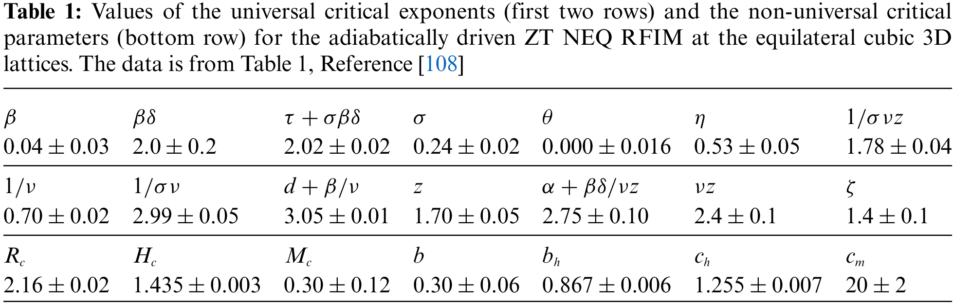
Previous theoretical and numerical studies [28,35,84,89] have shown that the adiabatically driven ZT NEQ RFIM systems, situated at the equilateral (hyper)cubic lattices with dimension
In finite systems, the role of infinite avalanches is played by the spanning avalanches [27] spreading along at least one of the system’s spatial dimensions and, therefore, classified according to the number of dimensions they span as 1d, 2d, and 3d spanning avalanches (further classified in [27] into critical and subcritical 3d spanning avalanches [173]). As shown in the comprehensive work investigating the ZT NEQ RFIM on finite equilateral 3D cubic lattices [108], the distributions of the number
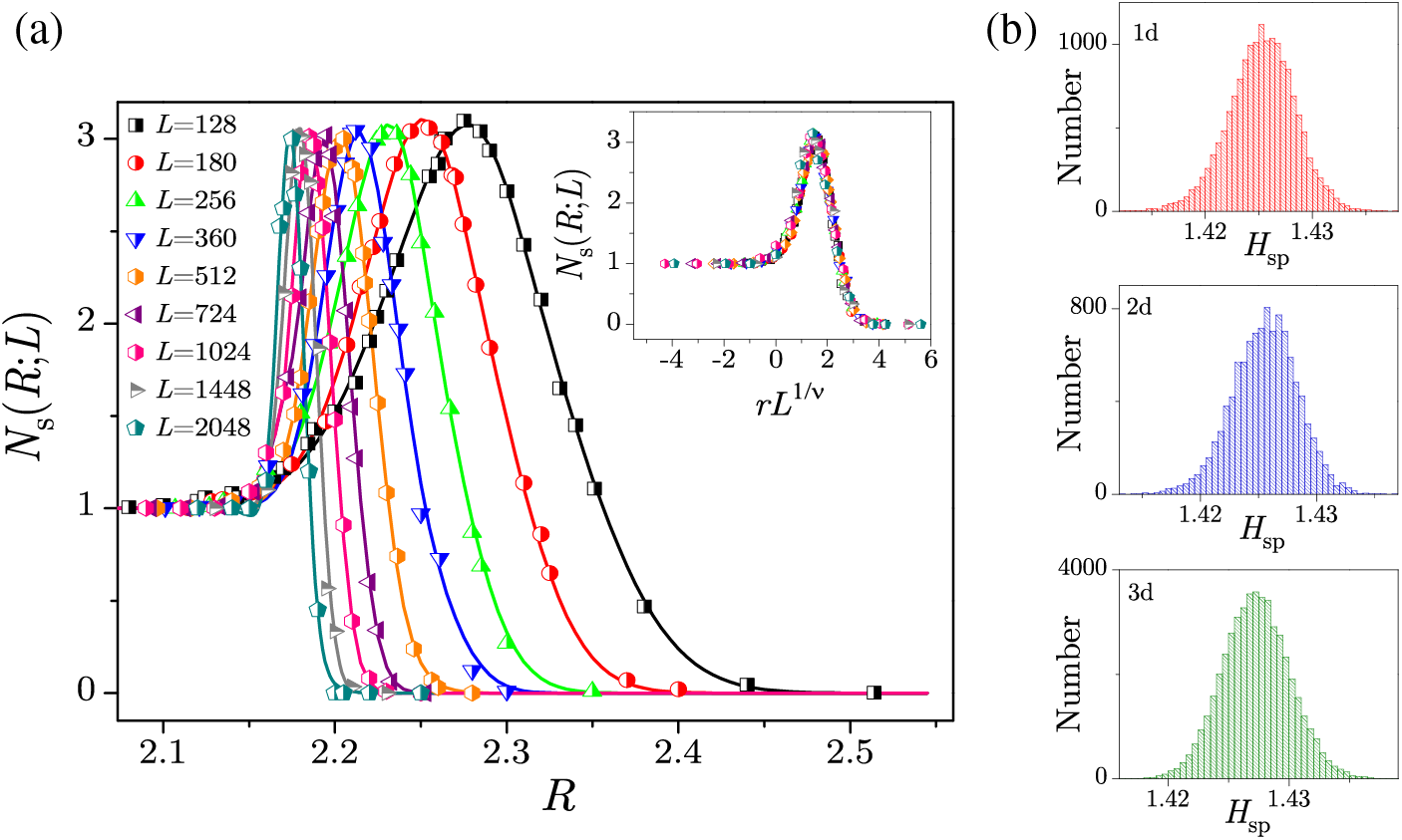
Figure 1: The total number of spanning avalanches per single run,
see in the inset of Fig. 1a, where
depending on parameters H,
Results published in [108] are obtained in by-all-means extensive numerical simulations, averaged across up to
In the subcritical and transitional domains of disorder, the single-run magnetization curves have jump(s) that appear at the spanning field
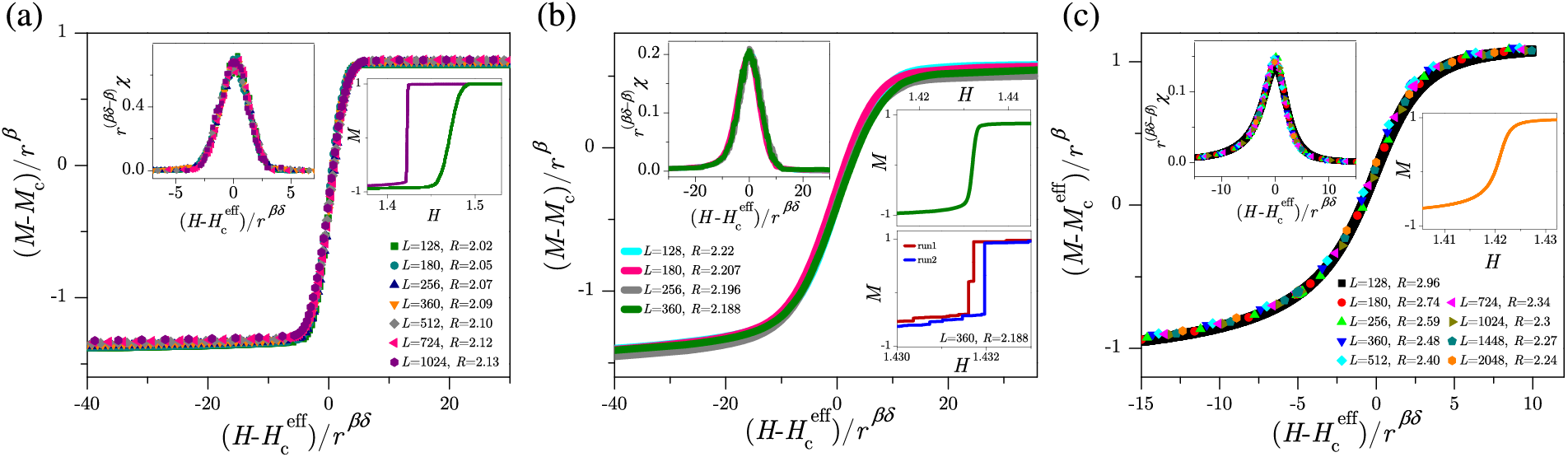
Figure 2: Main panels show the scaling collapses (12) of the averaged magnetization curves in the domains of disorder: (a) below critical, (b) transitional, between the critical and the effective critical, and (c) above the effective critical disorder, for a constant value of
Averaged magnetizations and magnetic susceptibility curves for finite systems of lattice size L, according to [27,108], follow the scaling forms
where
The distributions of avalanche parameters are cutoff-ending power-laws of the distributed parameter which depend on the underlying values of disorder R and lattice size L. Considered as the generalized homogeneous functions of their arguments, these distributions should follow finite-size scaling predictions in three equivalent forms, two of which, for the integrated size distributions and according to [27,108], read
and
where
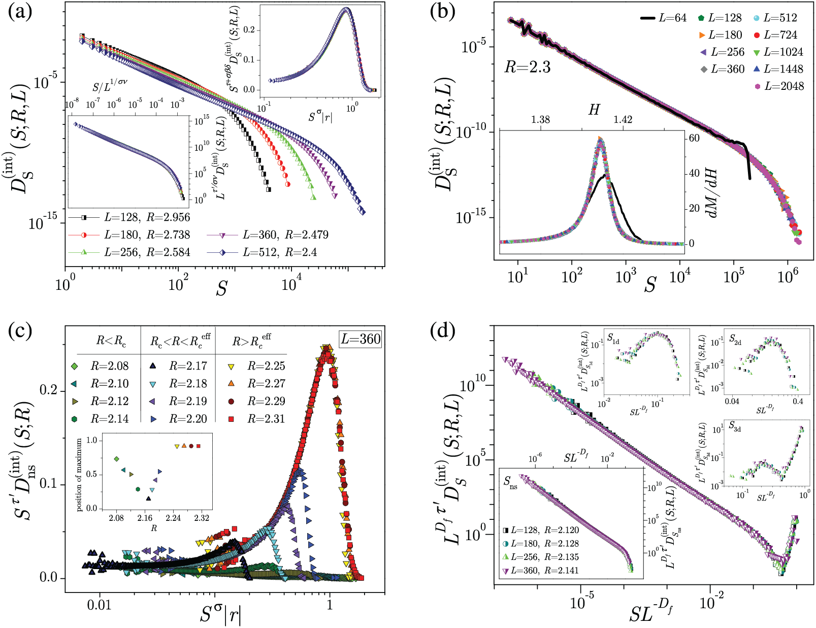
Figure 3: (a) Presented integrated size distributions are all from the supercritical domain of disorder and correspond to the
for infinite systems, following from (15) in the
On the other hand, according to the same Reference [108], in the subcritical and transitional domains of disorder, the L-independent scaling (16) is violated, while the L-dependent scaling conjectures (14) and (15) remain in effect, see Fig. 3c. In the main part of Fig. 3d we illustrate the collapsing (14) in the subcritical disorder domain of the integrated size distribution of all avalanches
and
predicting their collapsing when
The integrated correlation functions, measuring the probability per spin that flipping of the spin initiating the avalanche will cause the flipping of spins at the distance
Here
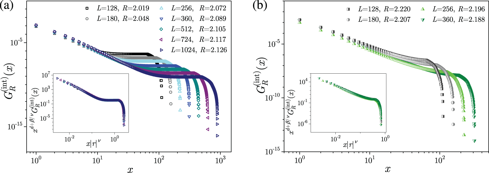
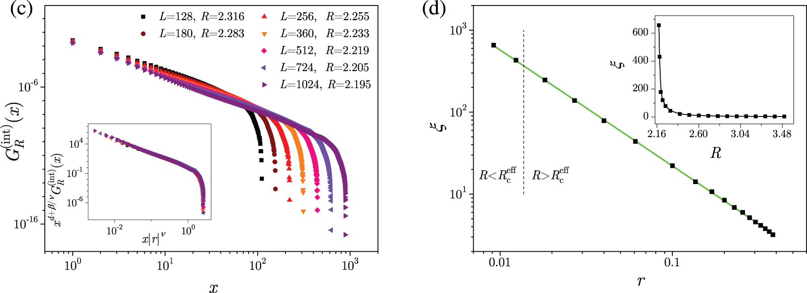
Figure 4: Integrated correlation functions
4.2 Adiabatically Driven ZT NEQ RFIM on Two-Dimensional (2D) Lattices
The question of whether the adiabatically driven ZT NEQ RFIM on 2D quadratic lattices exhibits nontrivial critical behavior remained open for almost 20 years. This puzzle was initiated by the Mermin-Wagner theorem [174] which proved the absence of coexistence of two ferromagnetically ordered phases in isotropic Heisenberg models [175] in
Complementary to the preceding theoretical issues stood the question of whether the real 2D disordered ferromagnetic samples exhibit critical behavior until being experimentally confirmed in studies [184,185], opening a wide venue for further fundamental experimental and theoretical investigations of the 2D disordered ferromagnets and their applications.
4.2.1 The Case of Quadratic Lattices
Numerical simulations reported in [89,90], performed for the system sizes up to
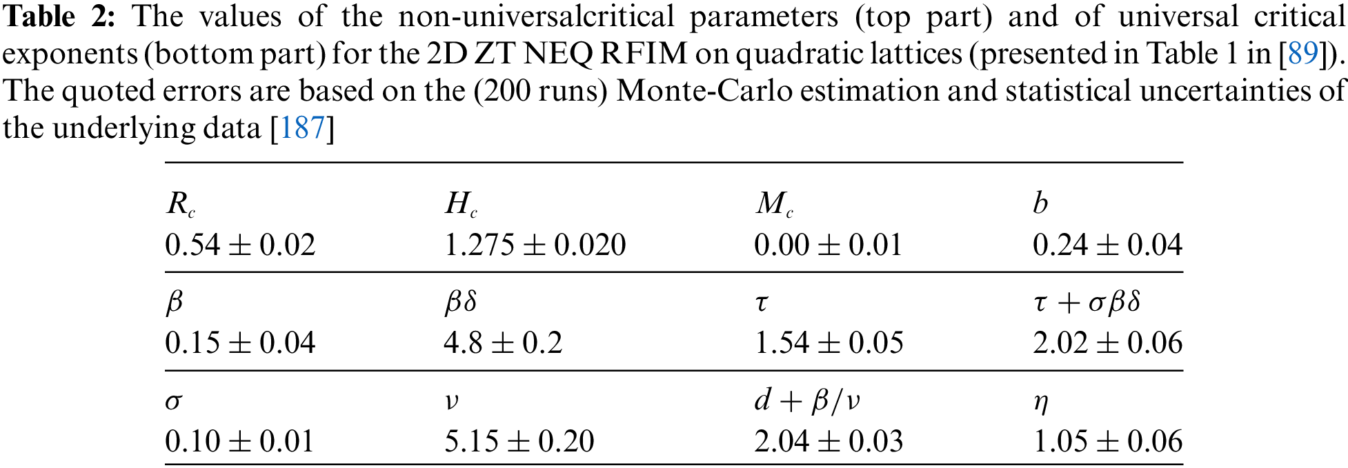
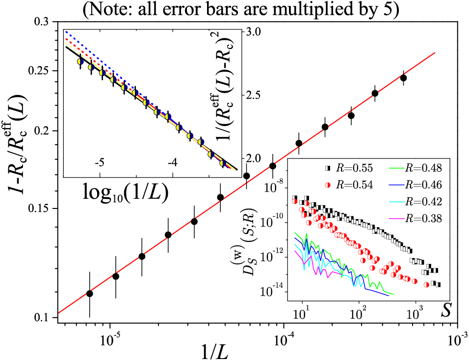
Figure 5: Effective critical disorder
In Fig. 6a, we presented (the rising part of) the magnetization curves
which follows from (12) in the
and Eq. (13). The collapsing of
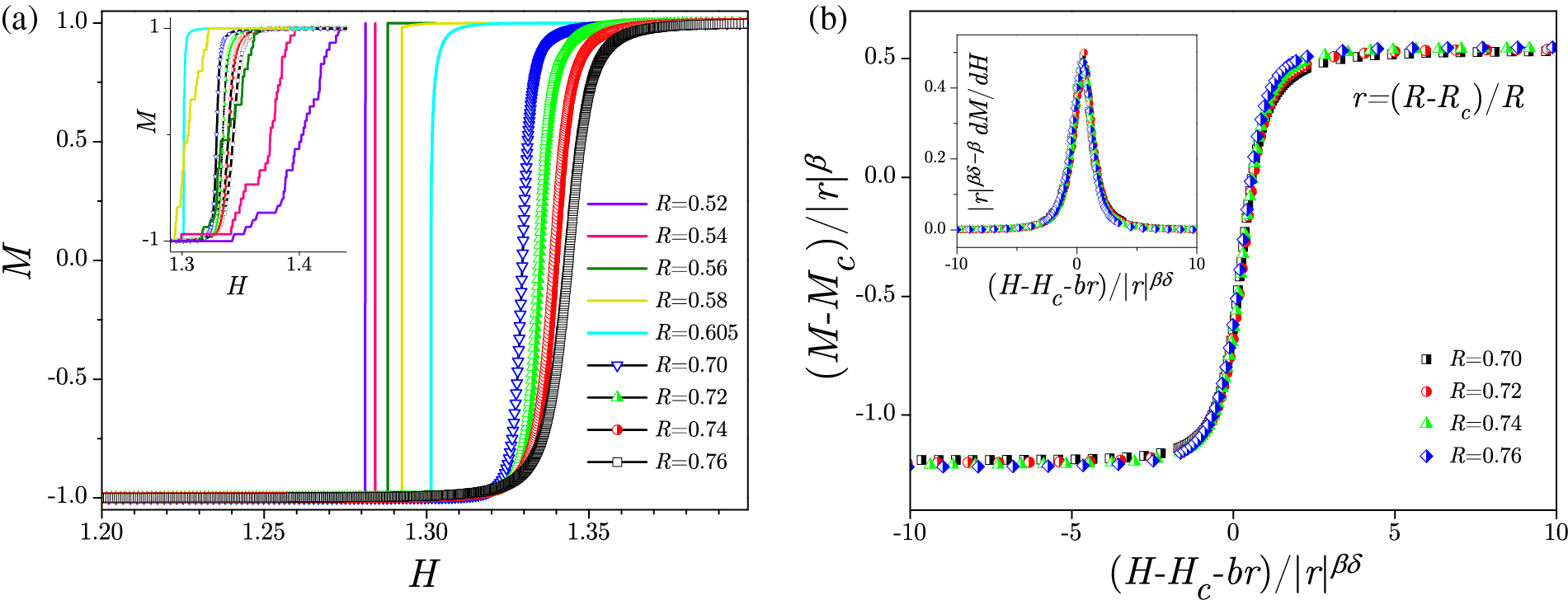
Figure 6: (a) Rising part of the magnetization curves
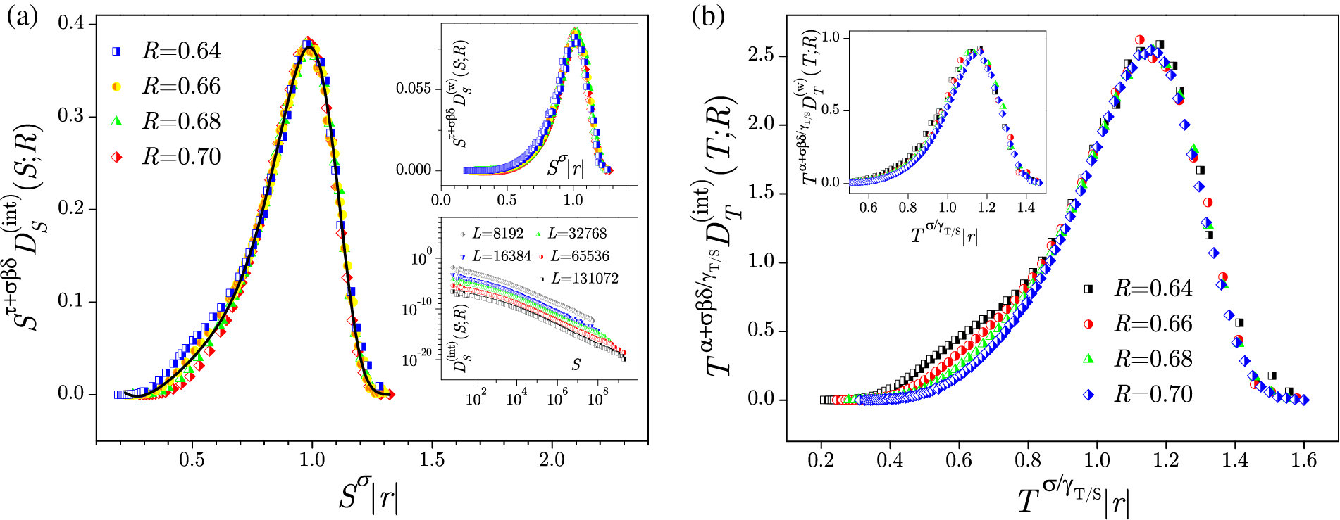
Figure 7: (a) The main panel shows the collapsing of the integrated distributions of avalanche size collected at
following from Eq. (15) in the
collected in complementary windows
of the size distribution
The behavior of the correlation function
where
where
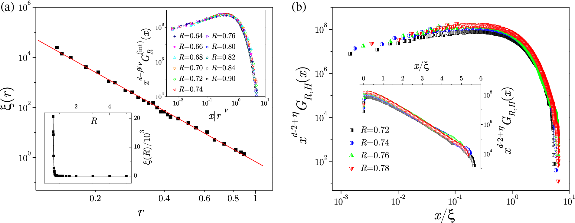
Figure 8: (a) The main part shows power-law divergence
4.2.2 Spanning Avalanches on Quadratic Lattices
Below the effective critical disorder
enabling their collapsing presented in the panel (b), and indicating that
with
and is presented in the inset of Fig. 9b. Due to scale invariance, the clusters of spins flipped during a spanning avalanche are fractals; their fractal dimension
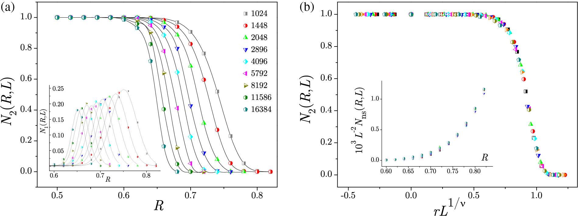
Figure 9: (a) Main part and inset show the number of spanning avalanches per single run,
Figure 10: Plots of a
Spanning avalanches cause bumps in distributions and jumps in magnetization
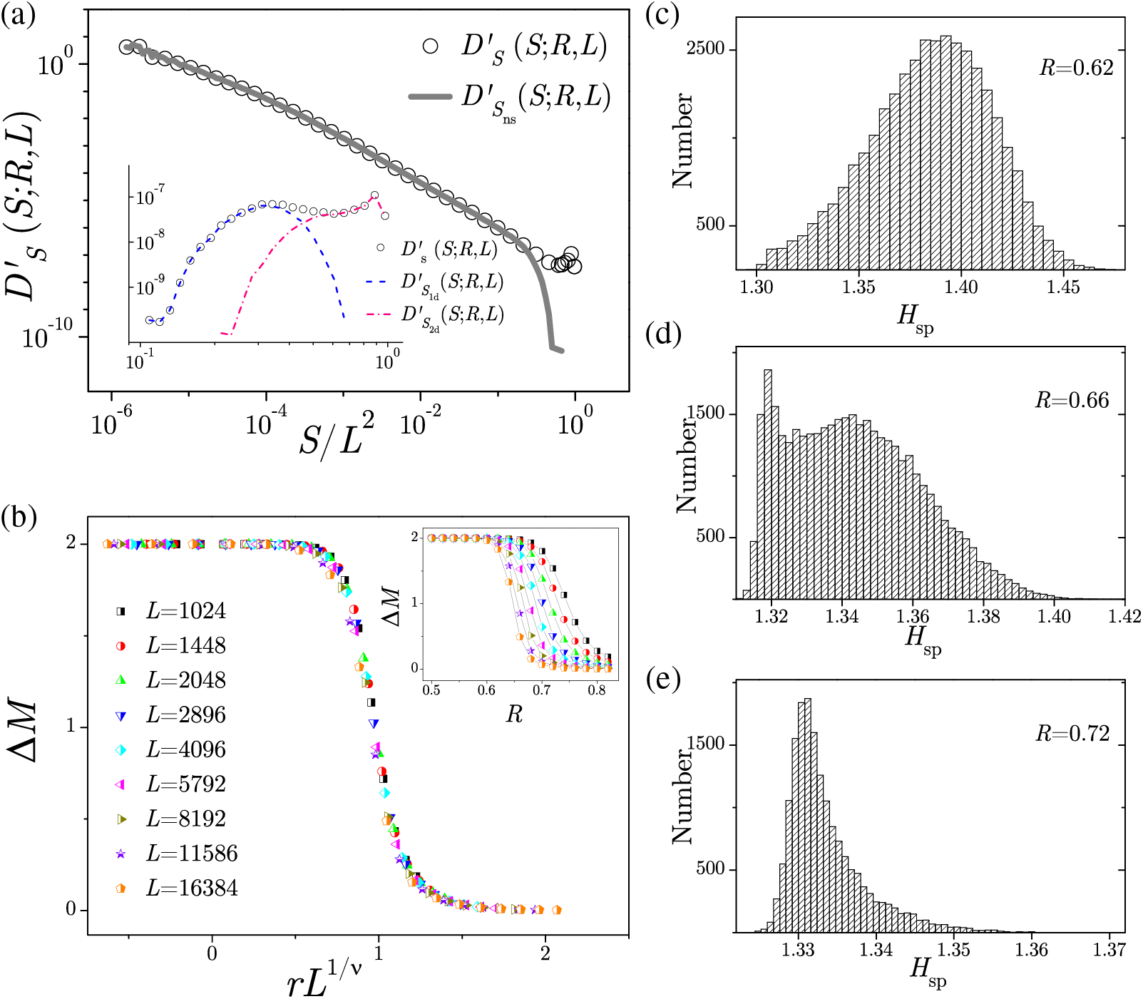
Figure 11: (a) (Scaled) size distributions of all avalanches (circles), nonspanning avalanches (full line), and spanning avalanches in the inset. (b) Magnetization jumps
4.2.3 The Case of Triangular and Hexagonal Lattices
Besides quadratic, the ZT NEQ RFIM can be studied on other 2D lattices with translation symmetry, but with different topology of elementary cell, e.g., with different number of nearest neighbors given by the coordination number
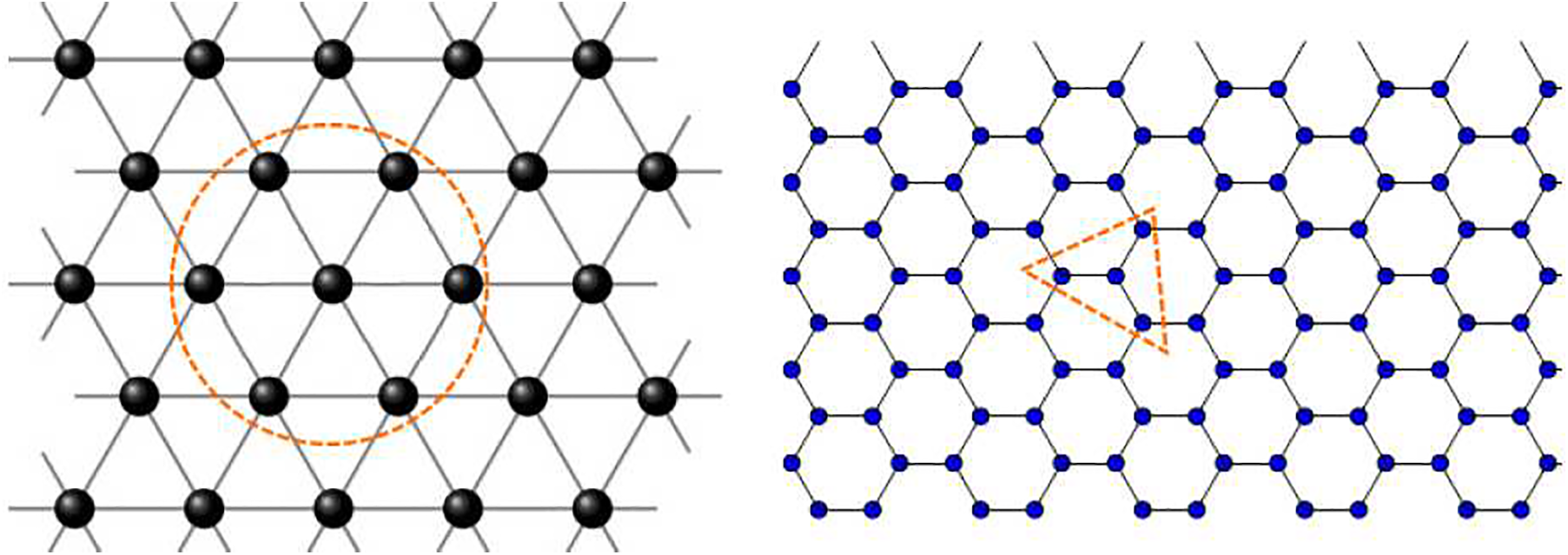
Figure 12: Triangular (left) and hexagonal (right) lattices. The right panel is Fig. 1 from [103]
The studies [100] on triangular and [103] on hexagonal lattices gave partial answers to the conjecture introduced in [135] that the coordination number
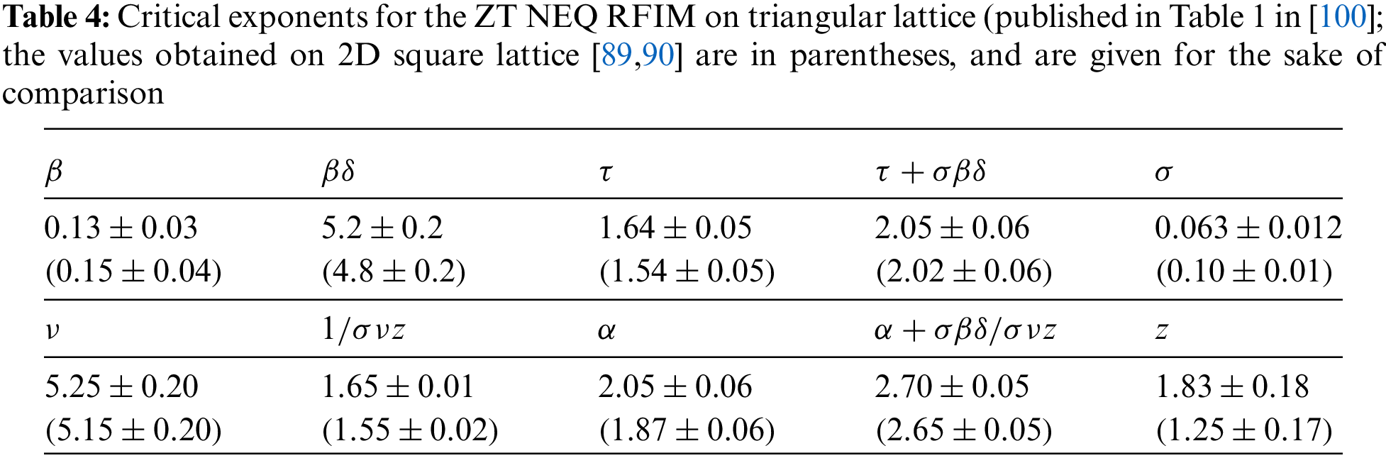
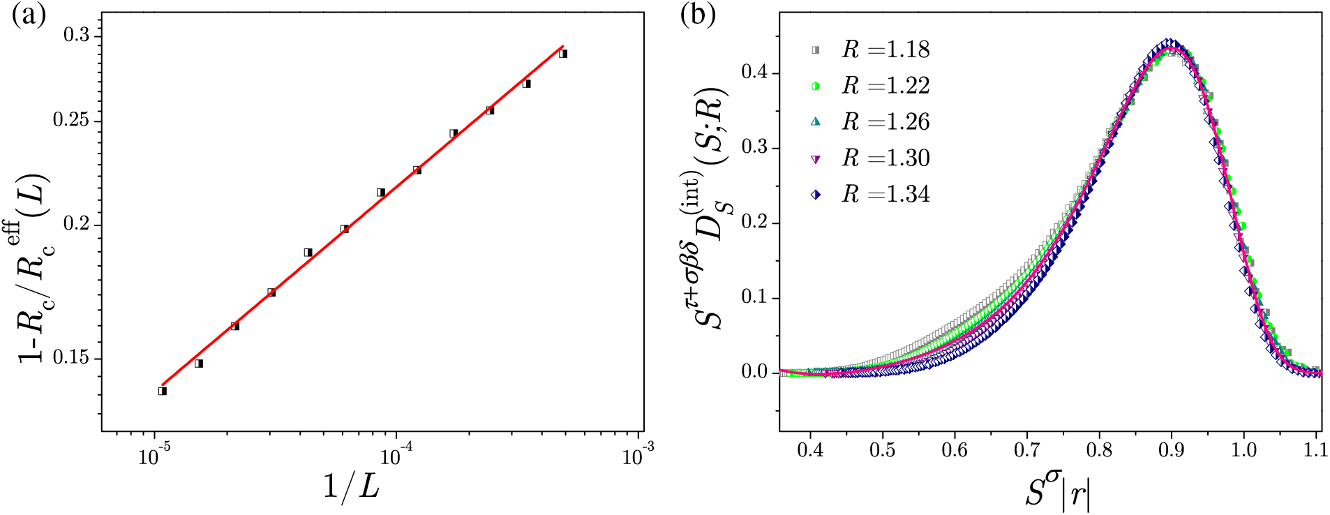
Figure 13: (a) Effective critical disorder
4.3 Crossover from 3D to 2D ZT NEQ RFIM Systems
The dimensional crossover from three to two spatial dimensions has been studied so far both experimentally [22,188] and in equilibrium models [189–192], where it has been established that the systems with constant thickness
The 3D to 2D dimensional crossover in ZT NEQ RFIM was studied in [110–112] on nonequilateral 3D
for the effective critical disorder
predicting the effective magnetic field
for
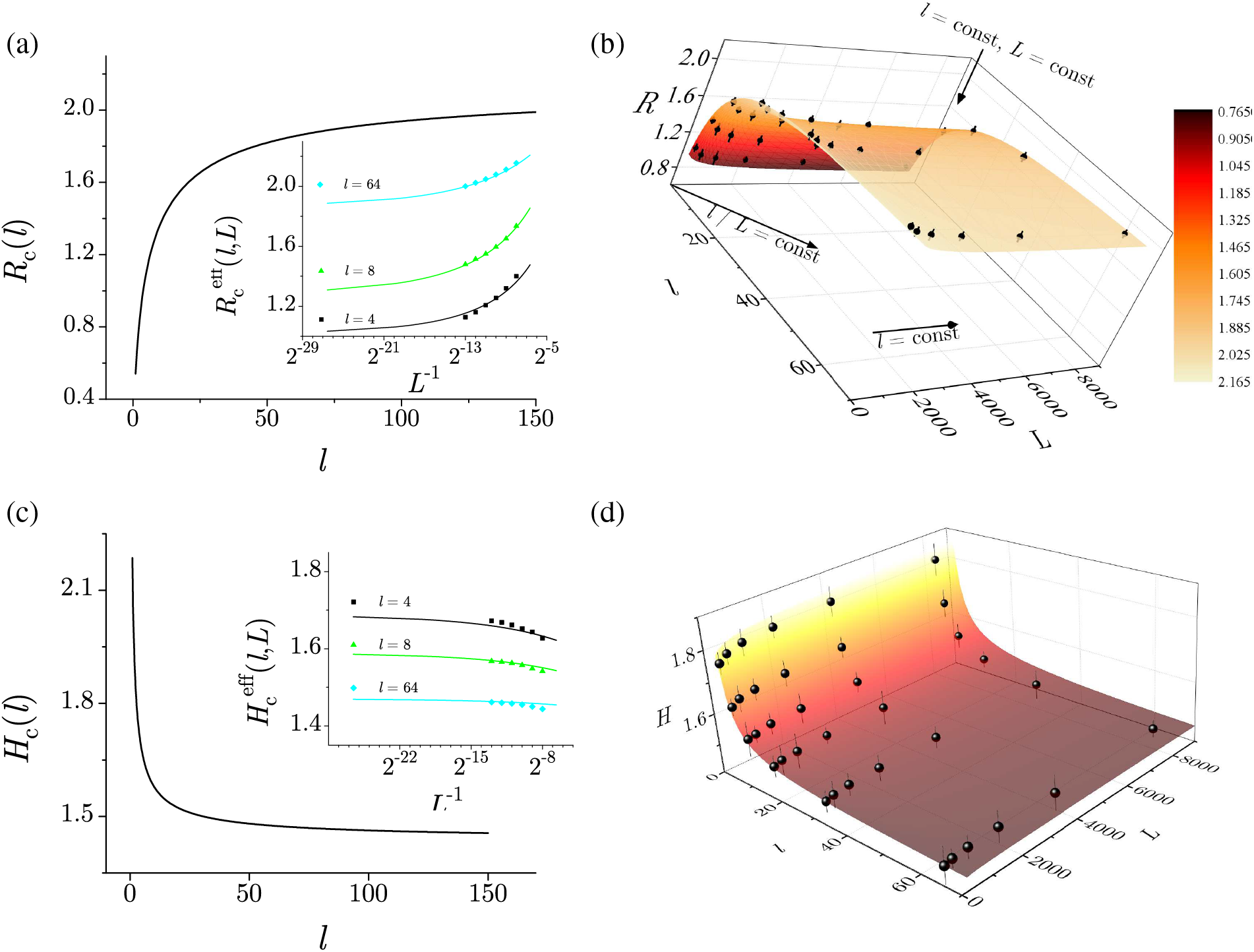
Figure 14: (a) Full line in the main left panel shows the
In Fig. 15, we show the integrated size distributions collapsed according to three types of scaling
predicted for
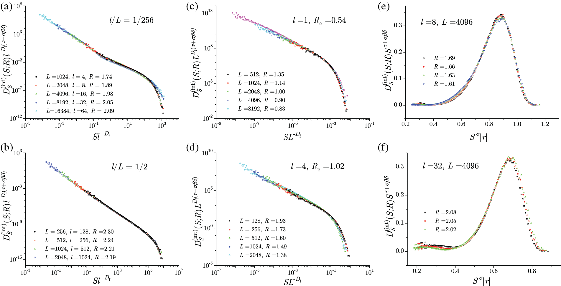
Figure 15: Data collapsing of the integrated size distributions
In the case of a small aspect ratio
4.4 Thin 3D Systems with Open Boundaries
Among various RFIM systems, thin systems with open boundaries play a distinguished role being the most appropriate model for real thin magnetic systems. The response of thin RFIM systems displays a lot of peculiarities studied in [111] on the
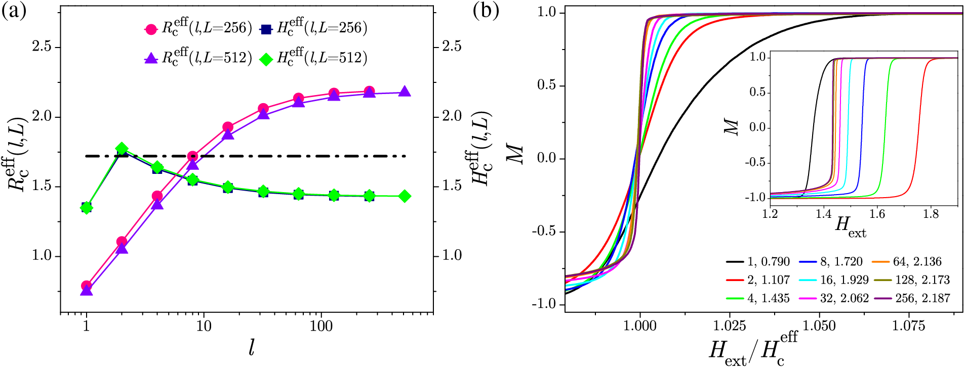
Figure 16: (a) Effective critical disorder
In the left column of Fig. 17, we show the size distributions
that, besides on
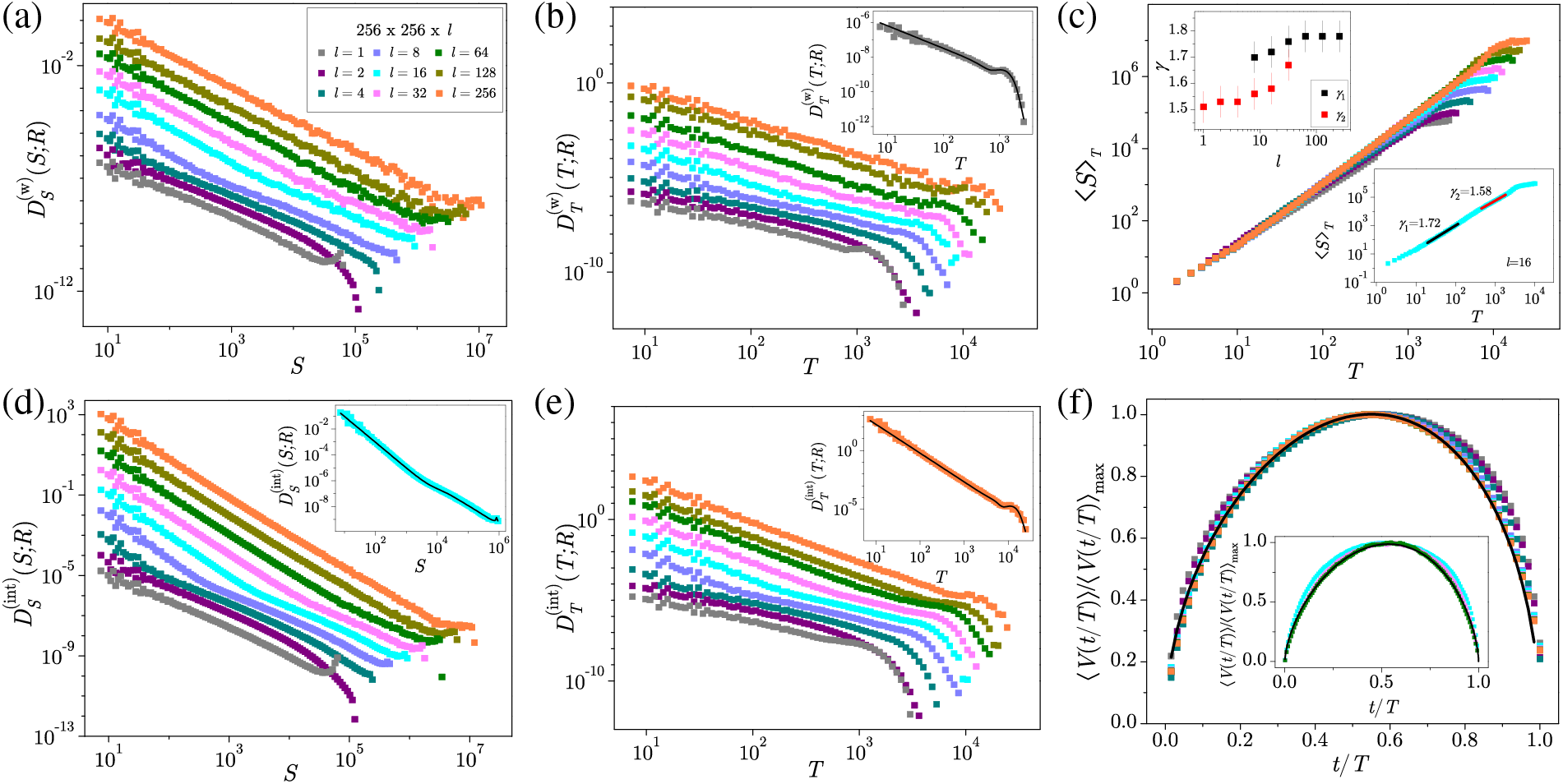
Figure 17: Distributions for thicknesses
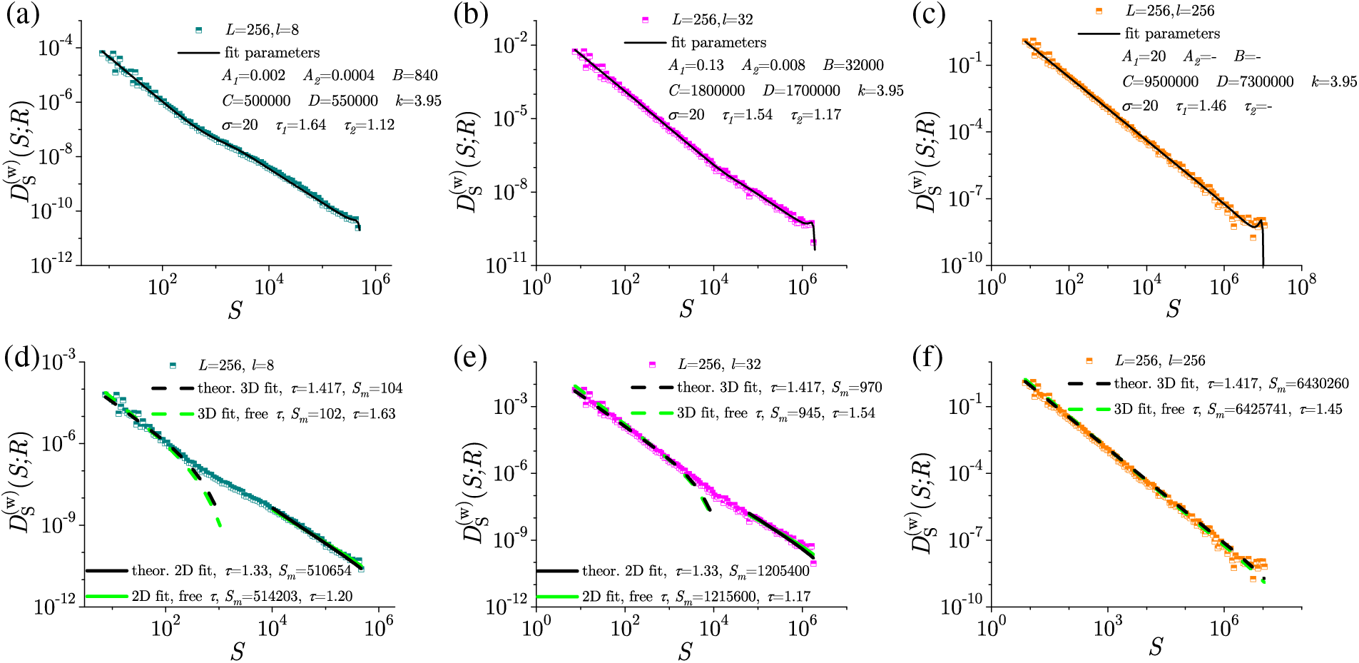
Figure 18: In the central part of the hysteresis loop, the distribution of avalanche size
Two scaling regions also appear in graphs showing the power-law correlation
The average shapes,
depending on an additional parameter
5 Finite Driving Rate Induced Spatio/Temporal Merging of Avalanches
5.1 Finite Driving Rate Effects on 3D Systems
In comparison with the widely utilized adiabatic driving, presented in previous sections, driving a disordered ferromagnetic system at a constant rate provides a more realistic scenario that is very useful for analyzing experimental data. In this type of driving, the external magnetic field is incremented/decremented along rising/falling part of the magnetization curve by a constant amount
As an example, three signal samples from the numerical simulations of equilateral 3D ZT NEQ RFIM driven at finite rates in each of the related regimes are displayed in Fig. 19b, together with relevant avalanche size distributions depicted in Fig. 19a. Therefrom, it is evident that in the slow driving regime, the same behavior is observed as for the cases of adiabatic and quasistatic driving, manifested by overlapping of all avalanche distributions, regradless of the driving protocol employed. However, when driving rate increases, a departure from this tendency is observed, being the most noticeable in the fast driving regime.
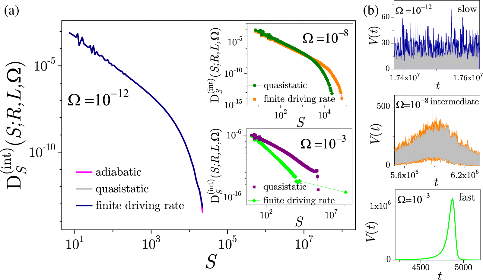
Figure 19: (a) Avalanche size distributions for
Because the dynamics of avalanches are significantly impacted by the driving rate, it is appropriate to analyze the driving rate effects on the systems that are large enough and have sufficiently high disorder (e.g.,
where
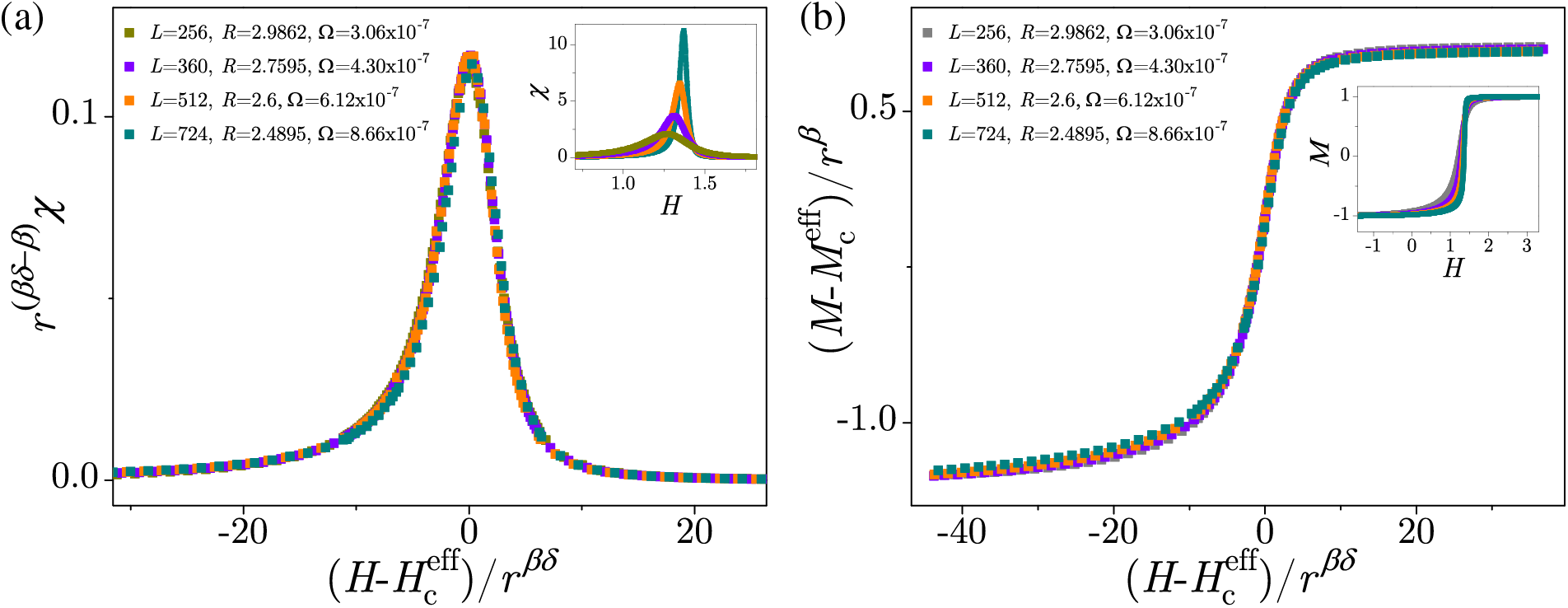
Figure 20: Scaling collapses of susceptibilities (a) and magnetizations (b) for system with parameters satisfying the conditions
As already mentioned, the avalanching activities are more difficult to analyze at the finite driving rate because of the merging of separately nucleated avalanches into system activity events (in this section for simplicity also referred to as avalanches). Such merging enlarges avalanches changing the shape of their distributions by e.g., promoting 1d into 2d spanning avalanches causing them to ‘flow’ from the first into the second distribution (and likewise for 2d and 3d spanning avalanches). So, in the intermediate driving regime, the distributions of 1d and 2d spanning avalanches become bimodal, see two top panels in Fig. 21a, making their scaling (and consequently collapsing) impossible. Due to the same reason, prominent dents appear at the cutoff start of the nonspanning avalanches’ distributions, see the bottom-right panel of Fig. 21a, arisen from the amalgamation of multiple nonspanning avalanches that eventually approach the system boundaries, turning into the spanning and being excluded from the distribution of nonspanning avalanches. Nevertheless, given that the system parameters satisfy the compatibility conditions
Figure 21: (a) The integrated size distributions of various types of avalanches (1d, 2d, 3d spanning, and nonspanning) collected at the driving rates from the legend, system size
with the rate-dependent values of the effective scaling exponents
Inspecting the flow of the exponents
The influence of the applied driving protocol on the spatiotemporal correlations of spin-flipping activity events with quite complex rate-induced behavior is another aspect that merits consideration. Results show that, provided the system parameters are tuned to satisfy the finite-size and rate-dependent scaling conditions, the spatial activity correlations follow rate-dependent scaling in all three driving regimes [148]. Temporal activity correlations, however, turn out to be highly sensitive to driving, so the collapsing of waiting time distributions is only achievable at very slow driving rates, and not possible for other rate choices. The increase in driving rate has a negative influence on various distributions of activity waiting times as well as on the activity average shapes that significantly deviate from slow driving and adiabatic behavior.
All spin flipping throughout the continuous system activity emerged at sufficiently high
Figure 22: Triggered activity correlation functions
When the system parameters are chosen so that the finite-size condition
is expected for the activity event correlation functions
Figure 23: Triggered activity correlation functions
The time that passes between any two subsequent system activity events is known as the total waiting time,
Given that the threshold-collapsing requirements
are met, together with the
introduced in [140] can be achieved in the slow driving regime for all types of the waiting-time distributions (see Fig. 24) with remark, however, that the increase of the driving rate causes distortions in the waiting time distributions
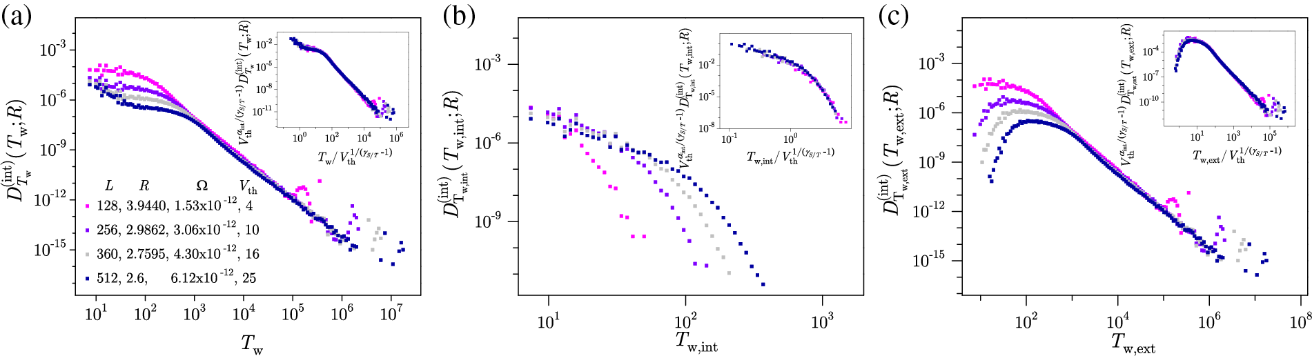
Figure 24: Distributions of (a) total, (b) internal, and (c) external waiting times, shown in the main panels, and their collapses (shown in insets) obtained in the slow driving regime with parameters satisfying the requirements (45) together with the
The correlation
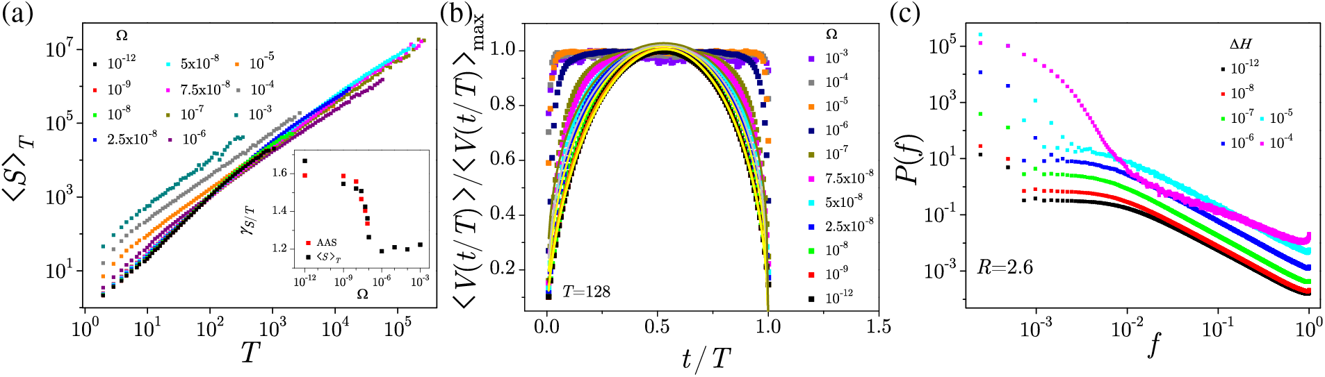
Figure 25: (a) Average size
In the finite-rate driving protocol, spanning activity events occur not just in the subcritical disorder domain, but also for higher disorders given the system is driven fast enough. This suggests that in systems of size L, there exists an effective critical driving speed
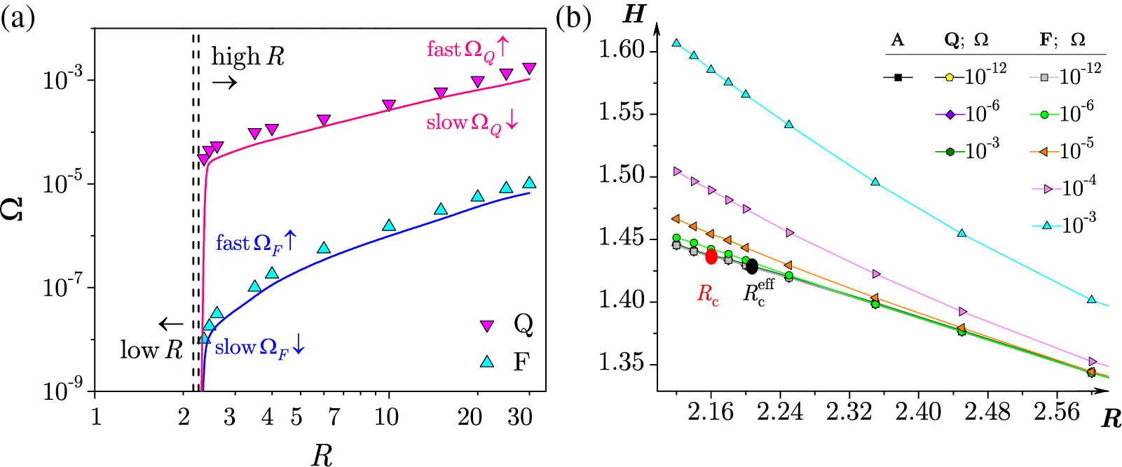
Figure 26: (a) Phase diagram showing the effective critical driving rate
Besides the critical driving speed, the flow of the effective critical magnetic field
5.2 Finite Driving Rate Effects on 2D Systems
The disorder of the system, which suppresses avalanche propagation, and the driving rate, which promotes it, pair up to produce the relaxation dynamics in the finite-rate driving protocol. Study of the effects of finite driving by the time-varying external magnetic field in the 2D disordered ferromagnetic systems is important from a conceptual and practical standpoint, due to the growing interest in novel miniature (quasi) 2D systems operating in the finite-rate driving regimes [149].
Following modified power-laws satisfying the scaling and data collapsing predictions introduced to describe the rate-dependent behavior of the model, it is demonstrated that it exhibits a dynamical phase transition with three distinctive regimes of driving rate identified in 2D, as in the case of 3D systems. Within the first regime of slow driving, the behavior of the system is approximately adiabatic from which it gradually deviates upon the increase of driving rate. At intermediate rates, owing to the temporal overlapping and/or spatial merging of avalanches, multiple spanning activity events are observed, whereas at fast driving rates, the system behavior is mainly influenced by the propagation of the biggest activity event as the single one spanning the system.
The new rate-dependent scaling forms are derived and implemented and their validity confirmed in extensive numerical simulations [149]. The system response follows a rate-dependent scaling in all three regimes of driving rate provided that the system parameters are tuned in compliance with the finite-size scaling condition
Within the constraints of the 2D system geometry, only two types of spanning avalanches can be realized, namely the 1d and 2d spanning avalanches [27,106], depending on whether the spanning spreads along only one, or both spatial dimensions; the remaining avalanches are classified as nonspanning. The numbers per single run of these two types of spanning avalanches,
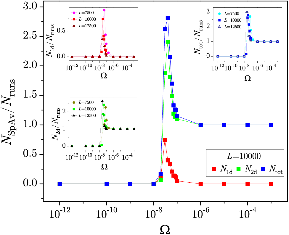
Figure 27: In the main panel are shown the number of spanning avalanches (1d, 2d and total) per single run
As was previously demonstrated in the 3D example, the presence of either disorder-induced or rate-induced spanning events in the system determines the shape of magnetization curves. Like in the case of 3D systems driven at a finite driving rate, adiabatic-like behavior is maintained at low driving rates, but at higher rates, a rate-induced deviation from the usual adiabatic curves is apparent. Modified scaling forms taking into account the rate-dependence of the general form of the invariant
and it has been numerically demonstrated that
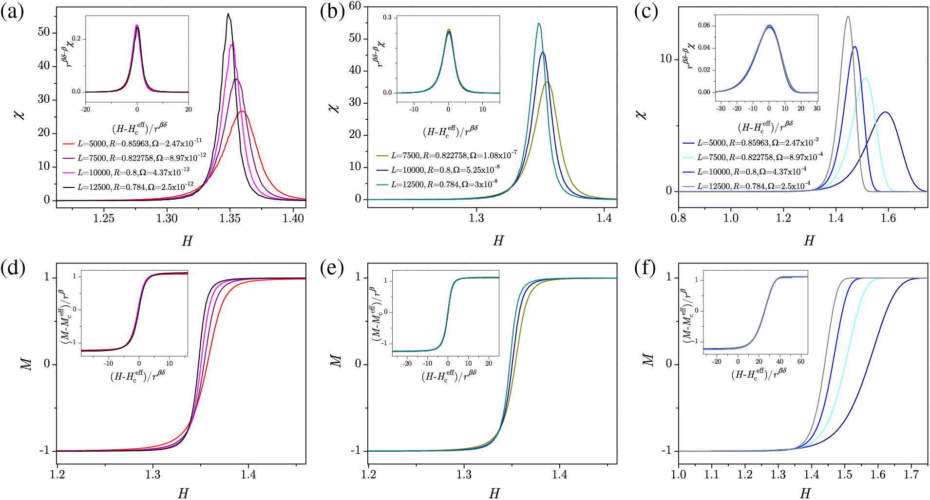
Figure 28: Susceptibilities are shown in the main panels of (a), (b), and (c) from the top row, while magnetizations are shown in the main panels of (d), (e), and (f) from the bottom row. All presented curves are acquired for the L, R pairs with both
Taking into account the effect of driving rate, similarly as it was done for the 3D case [130], the three types of scaling predictions for the integrated size distributions of nonspanning activity events (avalanches) are predicted in [149] given that the conditions
and
where
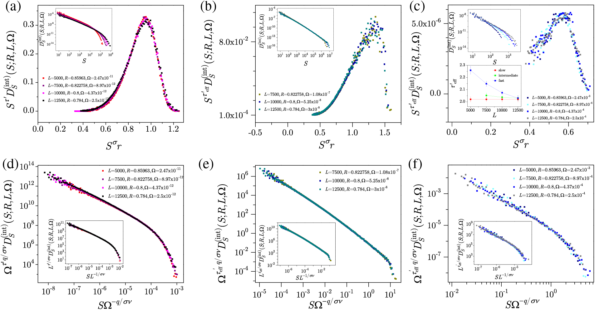
Figure 29: For the integrated size distributions of nonspanning activity events, shown in the top insets of panels (a), (b), and (c), we present their scaling collapses: of type (49) in top-row panels, of type (51) in bottom-row panels (d), (e), and (f), and of type (50) in insets of the bottom-row panels (d), (e), and (f). The systems parameters satisfy both
Fig. 30 evidences that all changes with
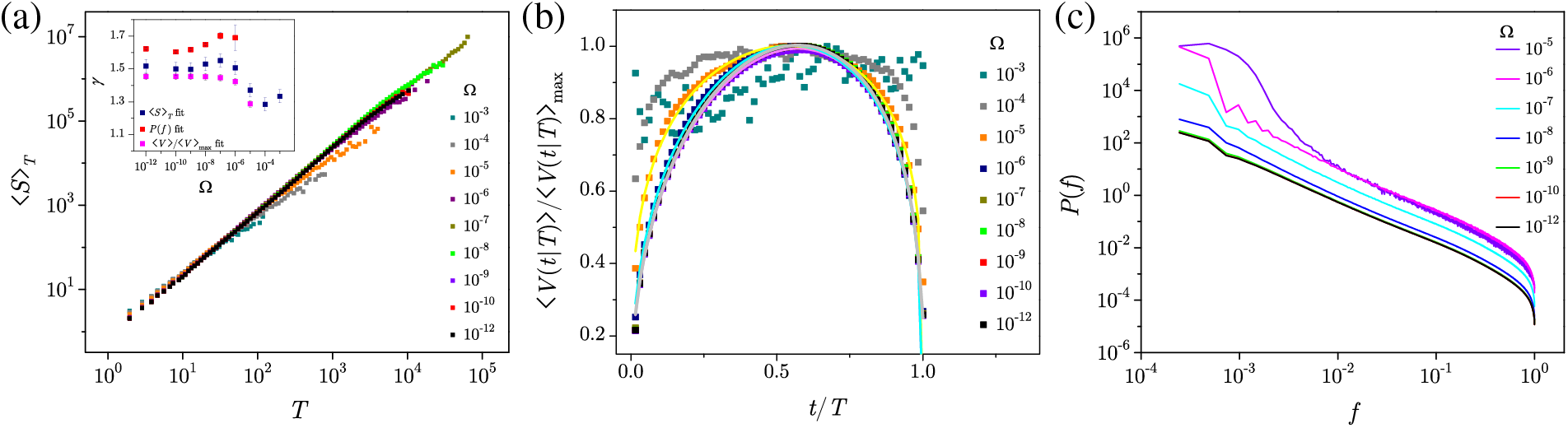
Figure 30: (a) Correlations between the average size
The preceding similarity trend continues for the integrated correlation functions which in the slow driving regime display adiabatic-like behavior illustrated in Fig. 8 for the 2D case, up to the cutoff end, after which the onset of a post-adiabatic plateau can be noticed, occurring for big inter-spin distances
as presented in Fig. 31, provided that both of the conditions
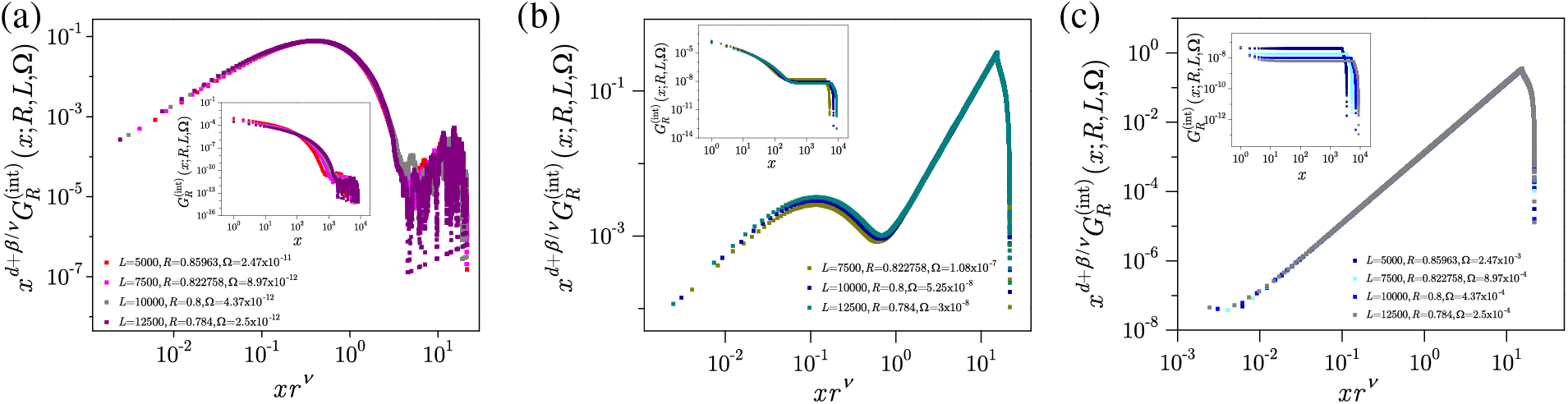
Figure 31: Main panels of (a), (b), and (c) show the scaling collapses of the integrated correlation functions
5.3 Crossover from 3D to 2D RFIM Systems Driven at a Finite Driving Rate
The imposed driving type together with the system thickness in the nonequilateral geometry profoundly affects its evolution, demonstrated in the magnetizations, coercive fields, distributions of avalanche sizes, correlation functions, average avalanche shapes and distributions of average avalanche size of a given duration [171]. While the driving rate remains in the slow regime, regardless of its thickness, a system behaves as being rate-independent and driven adiabatically. With the increase of the driving rate, the rate-sensitive behavior emerges, as a consequence of the initiation of multiple simultaneously propagating avalanches gathering and assembling into a complex response of system activity. This becomes even more intricate when the system’s thickness is in the transitional range, due to the coexistence of different types of avalanches, displaying both 3D and 2D effects described with pertinent effective rate-dependent exponents changing with the driving rate. Understanding this dimensional crossover is of considerable importance for the analysis of data obtained in experimental studies conducted on field-driven nonequilateral samples such as ferromagnetic strips, ribbons and thin films [194,195].
The dimensional crossover from 3D to 2D systems at finite driving rates is numerically studied in [171] so that for each system’s thickness the disorder is fixed above the critical line for adiabatic driving to ensure that the emergent critical behavior is solely attributed to the increased driving rates of the external field. The so-called transient thicknesses are characterized by the double-sloped distributions of avalanche parameters (such as sizes), which show the coexistence of two types of avalanches: purely 3D but small-sized avalanches and effectively 2D ‘squeezed’ avalanches, whose propagation is constrained by the system limits. Fig. 32 shows the integrated avalanche size distributions
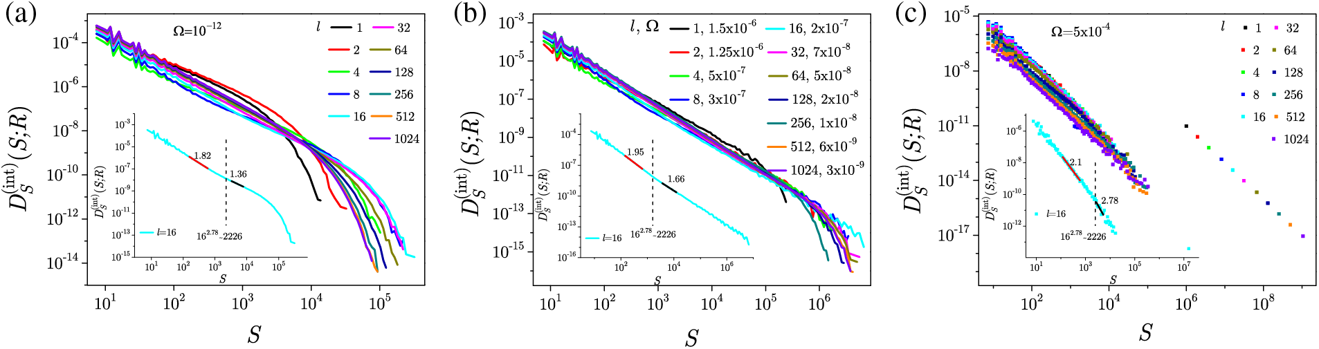
Figure 32: Integrated distributions
With some modifications in the transition from 3D to 2D with the systematic change of system thickness
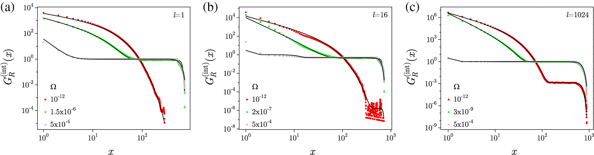
Figure 33: Integrated correlation functions in the slow, intermediate, and fast regimes for the representative thicknesses:
Fig. 34 shows average avalanche shapes on the time scale measured from the commencement of an avalanche divided by the duration of the avalanche T. These shapes are fairly symmetric for all system thicknesses for slow and moderate driving regimes, but flattening of their forms occurs for high rates, as seen in panel (c), because of the superposition of simultaneously propagating avalanches (also shown for the equilateral field-driven systems in [148]). With

Figure 34: Average avalanche shapes for avalanches with duration
5.4 Finite Driving Rate Effects on the Behavior of Thin 3D Systems
From a theoretical, experimental, and practical standpoint, thin disordered ferromagnetic systems pose a challenge in terms of comprehending their spatio/temporal evolution. Numerical simulations using the geometry of thin nonequilateral systems, where one dimension is much smaller than the other two, are used to address this problem over a wide range of driving rates and disorders [172].
The results suggest that the behavior that arises is the product of a non-trivial interaction between the three elements: the sample’s geometry, the disorder, and the employed driving protocol. Therefore, all commonly analyzed quantities exhibit rate-sensitive behavior, which appears in the generated signal’s shape and consequently all related behavior characteristics. In particular, this leads to changes in the distributions of avalanche parameters, correlation functions, and average avalanche shapes, which are characterized by the rate-dependent values of relevant exponents and coercive field values. Regardless of the system’s disorder, an almost adiabatic response happens during the slow driving, the deviation from which increases with the driving rate because many generated avalanches advance simultaneously (and possibly merge in space) forming activity events in the system response by their intricate superposition. This process is also influenced by the system’s geometry, which restricts the propagation in the direction of the system’s thickness, forcing avalanches to expand over the base plane and making them essentially two-dimensional.
The size distributions obtained for systems with a representative combination of thickness and disorder are exemplified in Fig. 35. System’s behavior for disorders below the effective critical is dominated by spanning avalanches, independent of its thickness. The occurrence of rate-induced spanning avalanches is evident with increasing rate, manifested in the modification of the distribution shape and the extension of the cutoff area to larger avalanche sizes. The windowed avalanche size distributions (comprised of avalanches that occur in the narrow magnetic field window selected so to facilitate comparison with the experimental data) are displayed in the middle panel of Fig. 35. Right panel of Fig. 35 shows the variation of
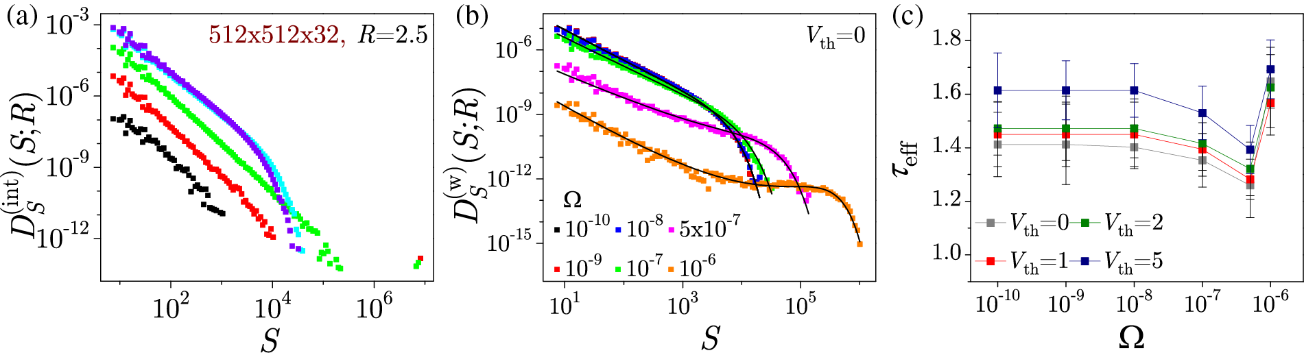
Figure 35: Integrated in (a), and windowed in (b) avalanche size distributions for the 3D systems with base
The integrated average avalanche shapes in the slow, intermediate, and fast driving regimes, as well as for different system thicknesses, are displayed in Fig. 36. It is evident that, at sufficiently low driving rates, the corresponding average shapes are symmetric and equal to adiabatic, irrespective of sample thickness. As the rate increases, the shapes begin to alter, becoming progressively more wide and flat due to temporal and/or spatial avalanche overlapping. Shape asymmetry happens at faster rates as well, and it’s more noticeable in samples with the lowest levels of disorder.
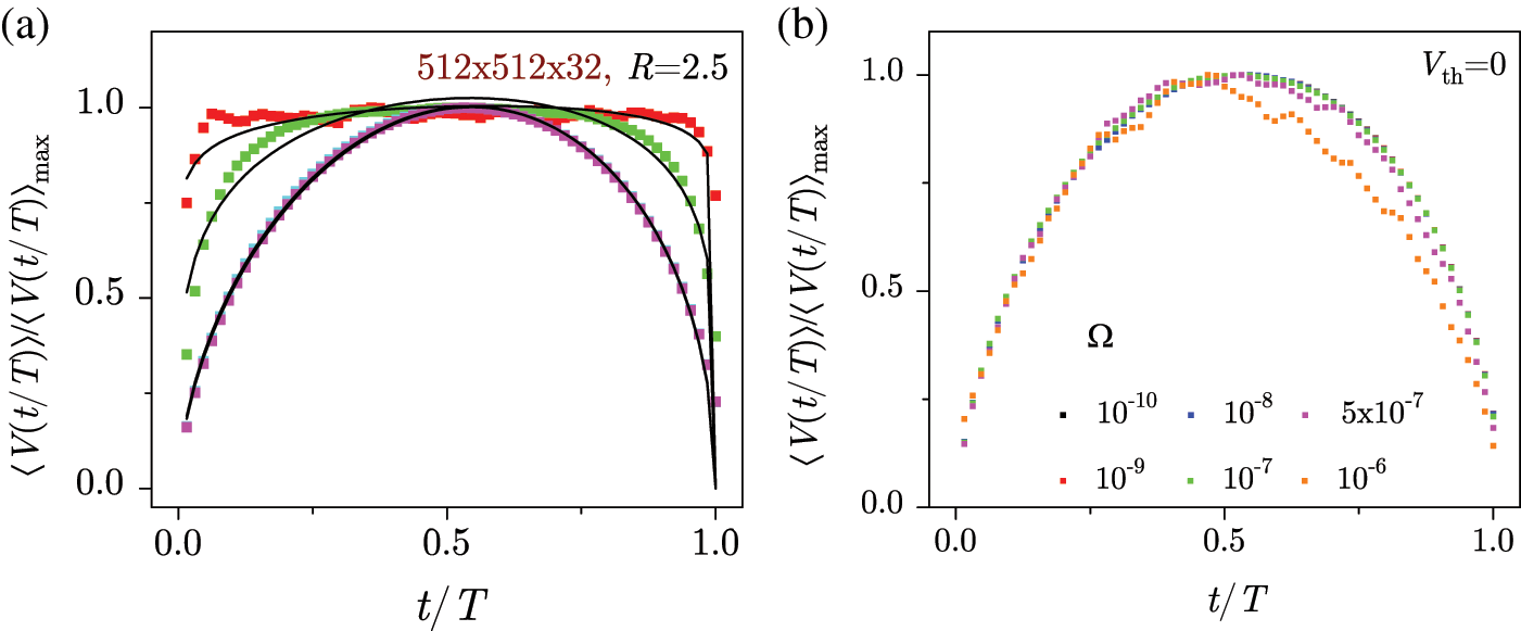
Figure 36: (a) Integrated average shapes of avalanches with fixed duration
In addition to the integrated, average avalanche shapes are also calculated for the avalanches formed in the magnetic-field window centered at the coercive field and having width corresponding to the
The triggered integrated correlation functions are displayed in Fig. 37 for a system of a chosen thickness, driven with a set of rates spanning the entire range of driving regimes. These functions have a characteristic spanning-induced plateau at 1. When spanning avalanches (i.e., activity events) are present, the system’s behavior is dominated by them, and as a result, the correlation function’s shape has a plateau at all system thicknesses. Conversely, the beginning of a post-cutoff plateau can be observed for very large disorders and the slowest driving rates. This plateau’s level increases with the rate until it eventually saturates and overlaps with the main plateau. Similar observations were made previously for the equilateral 3D systems with finite driving [148].
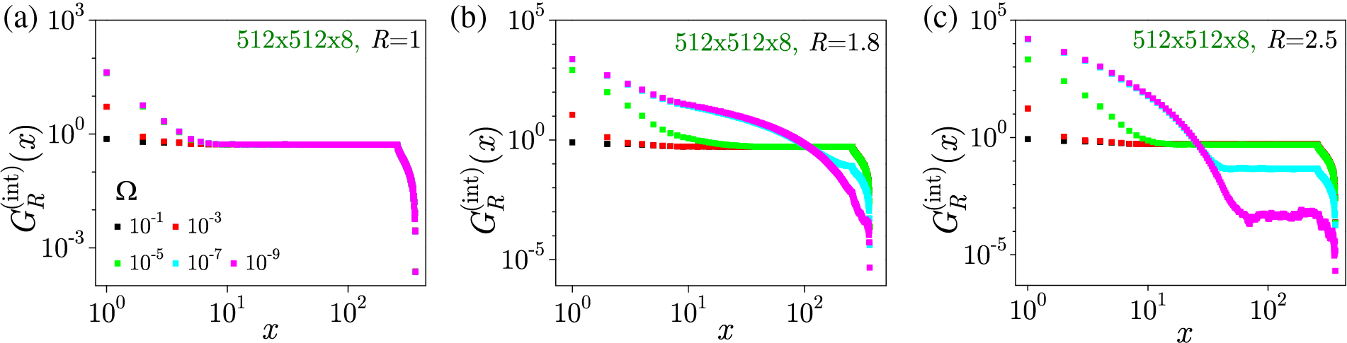
Figure 37: Variation with disorder R of the triggered integrated correlation functions driven at the rates shown in the panel (a) legend (valid for all panels) for systems with base
5.5 Disordered 3D Ferromagnetic Systems with Stochastic Driving
For simulating the complex phenomena with intermittent avalanche dynamics, deterministic external driving has typically been used with a well-defined protocol. In order to get as close as possible to the realistic scenario, a new driving method was proposed in the recent study [196], in which the external field takes stochastic increments within the framework of the ZT NEQ RFIM. This mimics realistic occurrences and potentially enables the results to be extended to the study of some difficult-to-achieve natural phenomena (e.g., earthquakes).
The results show that, provided the permitted range of field increments is small, the behavior is comparable to that of a constant-rate driven system. The system reacts in a complex way when the width of this range is expanded so that larger field increments are allowed. The scaling of the power laws is preserved and demonstrated for the distributions of avalanche parameters, average avalanche size of a given duration, and power spectra, whereas the deviations due to stochastic driving are found for the magnetizations and correlation functions.
Fig. 38 shows the integrated distributions of avalanche sizes, durations and waiting times. One can see that in the slow regime with small enough stochastic increments of the external field the distributions are practically the same as in the case of driving with a constant and small driving rate, while for the bigger stochastic steps, the differences start to emerge. Spanning avalanches are also generated, shown in the distributions as isolated points occurring after the cutoff region. As a consequence, the slope of distributions is also changed, reflected in the variation of the corresponding exponent values. The flows of the effective rate-dependent values of exponents are shown in pertinent insets against the logarithmic width
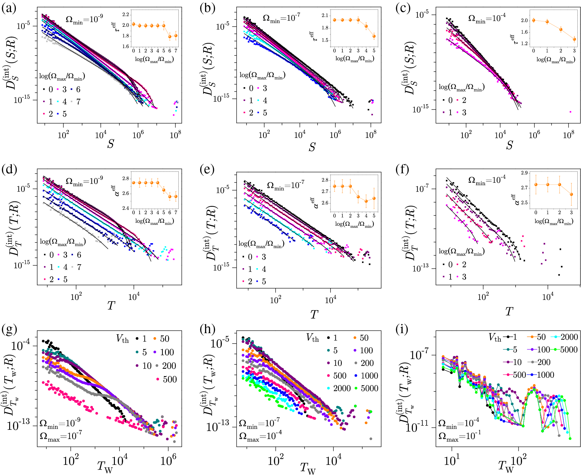
Figure 38: Integrated distributions of avalanche size (in (a)–(c) panels), duration (in (d)–(f) panels), and waiting time (in (g)–(i) panels) for the slow, intermediate and fast minimum stochastic driving rates
Additionally, in Fig. 39, preservation of the power-law dependence of average avalanche size of a given duration for the case of stochastic driving is showcased, as well as for the power spectra showing that this scaling holds only for narrow intervals of
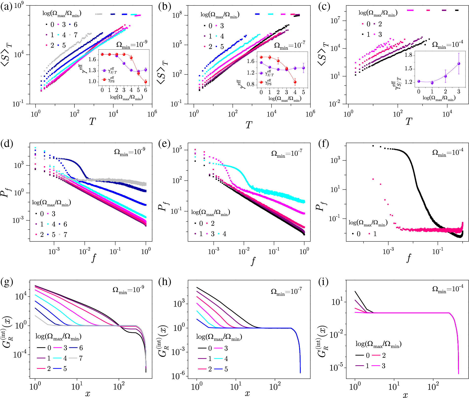
Figure 39: (a)–(c) Average size
Moreover, it is discovered that there is a high degree of consistency between the data from numerical simulations and the experimental data from fracture experiments, which demonstrate seismic-like behavior, and acoustic emission experiments of single crack propagation in inhomogeneous solids. This suggests that when complex systems generate intermittent, scale-free avalanche dynamics, there is a general underlying process that reproduces empirical rules, like Gutenberg-Richter’s law of earthquakes. Fig. 40 presents the comparison of the integrated energy distributions obtained in the numerical simulations of stochastically driven RFIM with the corresponding distributions obtained in acoustic emission experiments of a single crack propagation in inhomogeneous solid and fracture experiments [142] for which the seismic-like behavior is demonstrated.
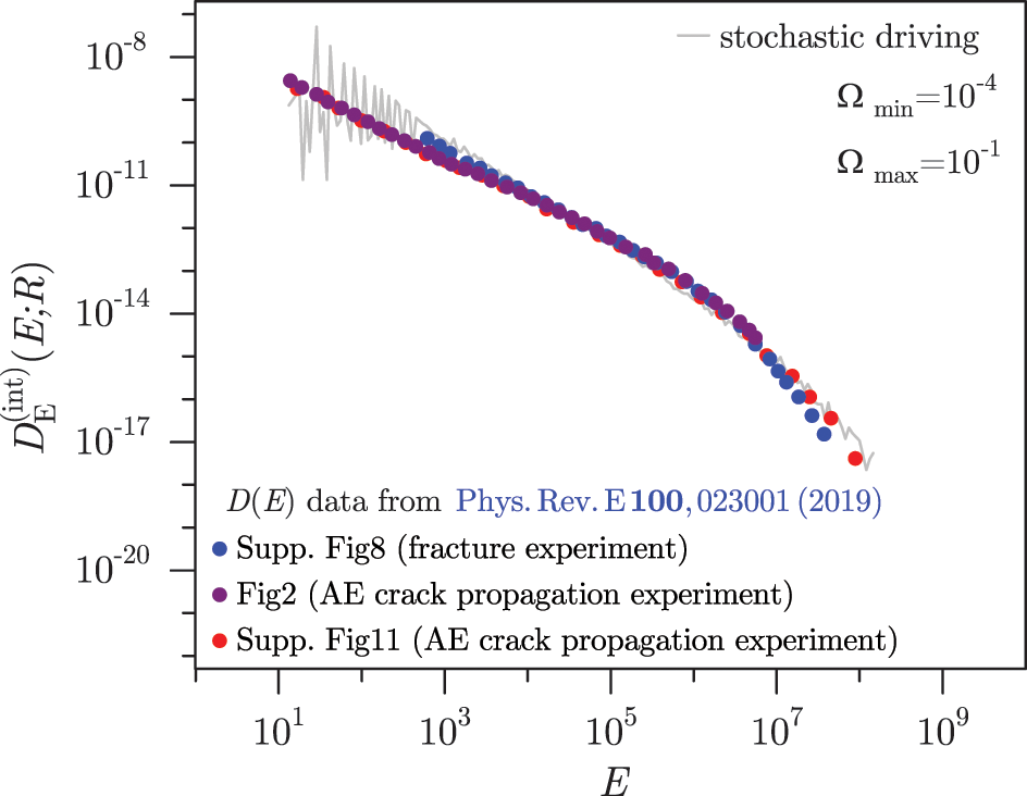
Figure 40: Comparison of integrated energy distributions, obtained in numerical simulations with stochastic driving (for system with size
6 Towards More Realistic Modeling: The Impact of Thermal Fluctuations and Demagnetizing Fields
Modelling driven disordered systems in a way that closely resembles experimental settings is a challenging endeavor due to the multitude of connected factors that impact their nonequilibrium dynamical behaviour. In a recent study on the effects of demagnetizing fields and thermal fluctuations of a thin ferromagnetic samples [164], the numerical simulations of the extended version of RFIM were conducted implementing novel algorithmic techniques. In this study, the magnetic field is cycled from the saturated hysteresis loop through a series of nested subloops gradually reducing to zero, forming along the demagnetization curve from the tips of all simulated subloops (see an example in the top left panel of Fig. 41).
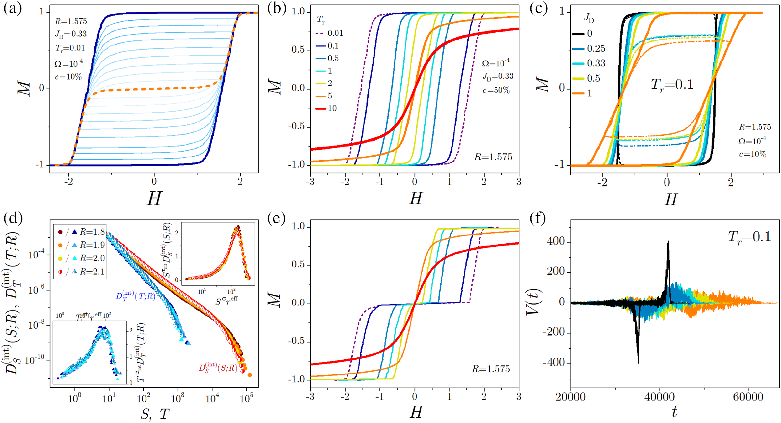
Figure 41: (a) Saturation hysteresis loop (full thick curve) with 10 subloops (shown out of 50 by thin full curves) and the demagnetization (dashed) curve. (b) Shrinking of single-run saturation magnetization curves with increasing relative temperature. (c) Single-run magnetization loops vs. simulation time
Using the thermal scenario (i.e., with the non-zero temperature) affects the values of the coercive field and remanent magnetization, causing the shrinking of the hysteresis loop and amplifying minor activity events. The temperature effects on the saturation loops and relevant demagnetization curves of the demagnetized system are shown in the middle panels of Fig. 41. The saturation magnetization loops exhibit a sharp rise at lower temperatures, gradually shrinking in width as temperature rises. This dissolves the hysteresis and brings the rising and descending branches into overlap, with the coercive field tending towards zero. In parallel, the characteristic plateau of demagnetization curve remains in the range of lower temperatures, gradually shrinking as the temperature rises and ultimately dissolving, smoothing the demagnetization curve.
Conversely, the demagnetizing field introduces the prolonged linear segments in the loops and alters the multifractal nature of the magnetization fluctuations. The right panels of Fig. 41 display the effects of varying the
The integrated distributions
where
6.1 Details of the Developed Numerical Algorithm
A more realistic modeling of the hysteresis loop phenomena in disordered ferromagnetic samples is introduced in [164] incorporating thermal and demagnetization field effects with possible extensions to heterostructures and thin films which are all the subject of numerous applications at the moment. This approach, which is computationally more efficient for thermal simulations than the one proposed in [166], selects a given fraction
In Fig. 42, we present the flowchart of a single-run algorithm used in [164], and its key points we summarize as follows:
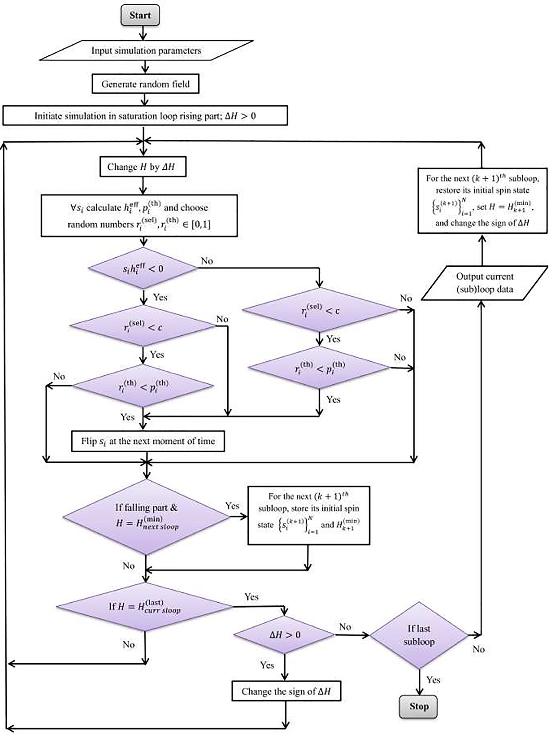
Figure 42: A flowchart of the single-run algorithm used in numerical simulations of the RFIM version incorporating demagnetizing field [164]. The dashed curve encloses the parallelized part of the algorithm. This figure is replotted from Fig. 7 from [164]
• The single-run simulation input parameters are the size
• For the supplied value of seed, the (Gaussian) random field configuration
• In each (new) time step the external magnetic field H is changed by
• After H is changed, all spins are in parallel tested and (possibly) flipped following the steps:
– the effective magnetic field
– random numbers
– for
∗ field-unstable,
·
·
∗ field-stable,
• When
• After H falls below the
Quenched averaging is performed over different RFCs using the same input parameters.
7 Collective Magnetization Fluctuations and Structure of Barkhausen Noise (BHN) in Experiments and Theory
As stated in the Introduction, the magnetization reversal in disordered ferromagnets is a stochastic process related to the motion, pinning and depinning of domain walls driven by slow ramping of the external magnetic field. Such motion is accompanied by a ‘crackling noise’ signal [201], known as the Barkhausen noise (BHN). It represents a time series of the magnetization changes during the reversal processes and is measured in the experiments. Given the avalanching dynamics related to the critical behaviour of the hysteresis-loop discussed above, the related BHN signals have a vibrant structure. For example, the BHN signal possesses long-range temporal correlations seen in the power spectrum and multi-scale fractality [33]; moreover, the sequence of avalanches represents another structured set characterized by Tsallis q-Gaussian distribution of the first returns [202]. Hence, the appropriate analysis of BHN signals can reveal valuable information about the stochasticity of the magnetization reversal process and quantify its dependence on relevant parameters [203]. In this section, we first demonstrate how the magnetization avalanches are extracted from the experimental BHN signal. Next, we show that the BHN distributions, measured in a nanocrystalline sample, are adequately described by the ZT NEQ RFIM with suitably selected parameters [168]. Furthermore, we give a more detailed description of the multifractal analysis of the BHN signals simulated by RFIM in different conditions. We define the appropriate quantitative measures and demonstrate their sensitivity to varied parameters by considering two representative examples.
7.1 RFIM Simulations Compared with the Real Samples’ BHN Avalanches
In this subsection, we give a comparison between the BHN emitted by a real sample and the RFIM version adjusted to give as close as possible matching with the experimental data reported in [168]. BHN recordings were performed with the experimental setup schematically depicted in Fig. 43 on an annealed (at
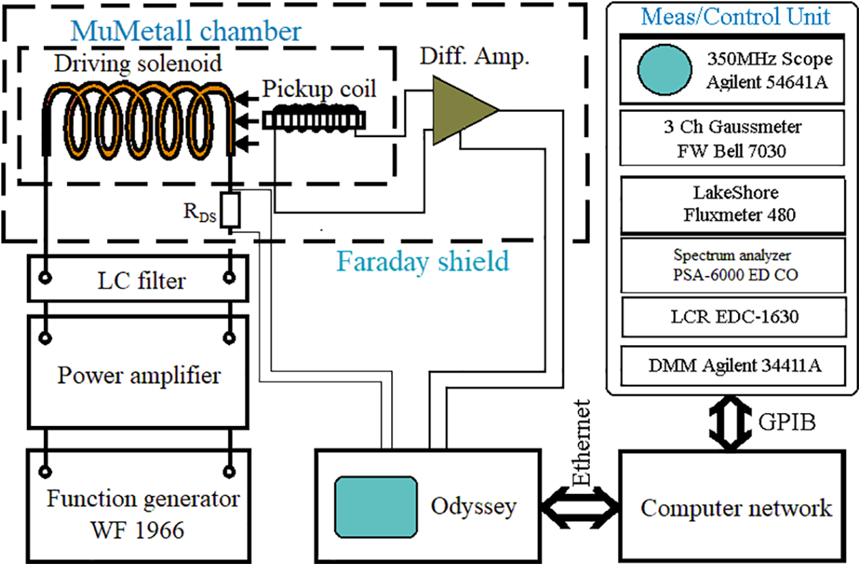
Figure 43: Scheme of the experimental setup used in BHN measurements. This is Fig. 1 in [168]
In BHN inductive recordings, the response signal is the voltage (i.e., electromotive force) induced in a pickup coil tightly wound around the sample. This voltage is amplified approximately
One period of the response signal, sampled 200,000 times per second at the resolution of 14 bits, is presented in Fig. 44 for seven driving frequencies from the range
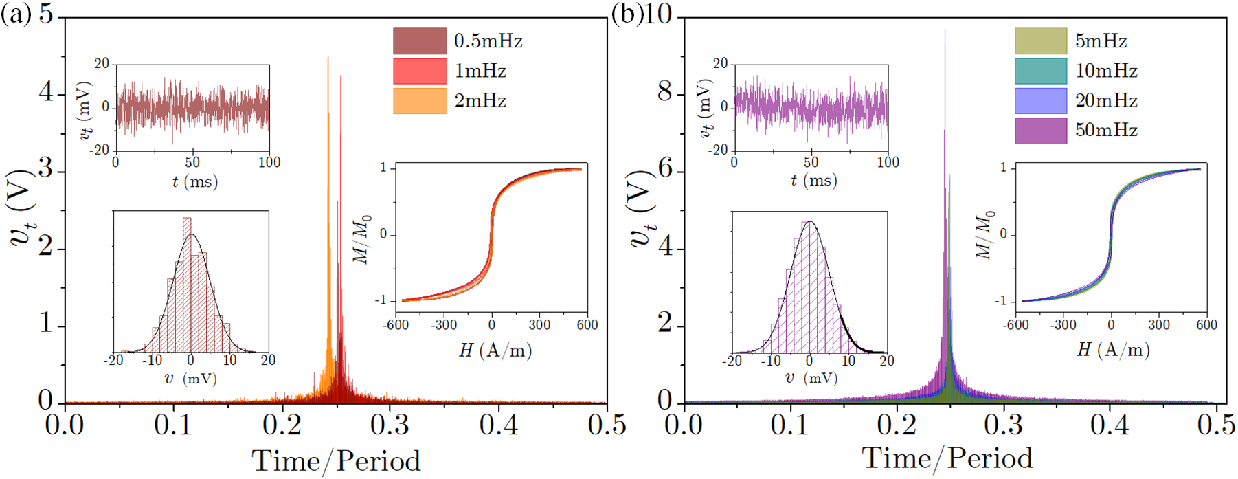
Figure 44: The main panels show one example of time profiles of the voltage response signal
To enable comparison with the experimental data, simulational units are scaled so as to provide the best match for the two types of data. This is achieved by dividing the simulational timescale by the factor
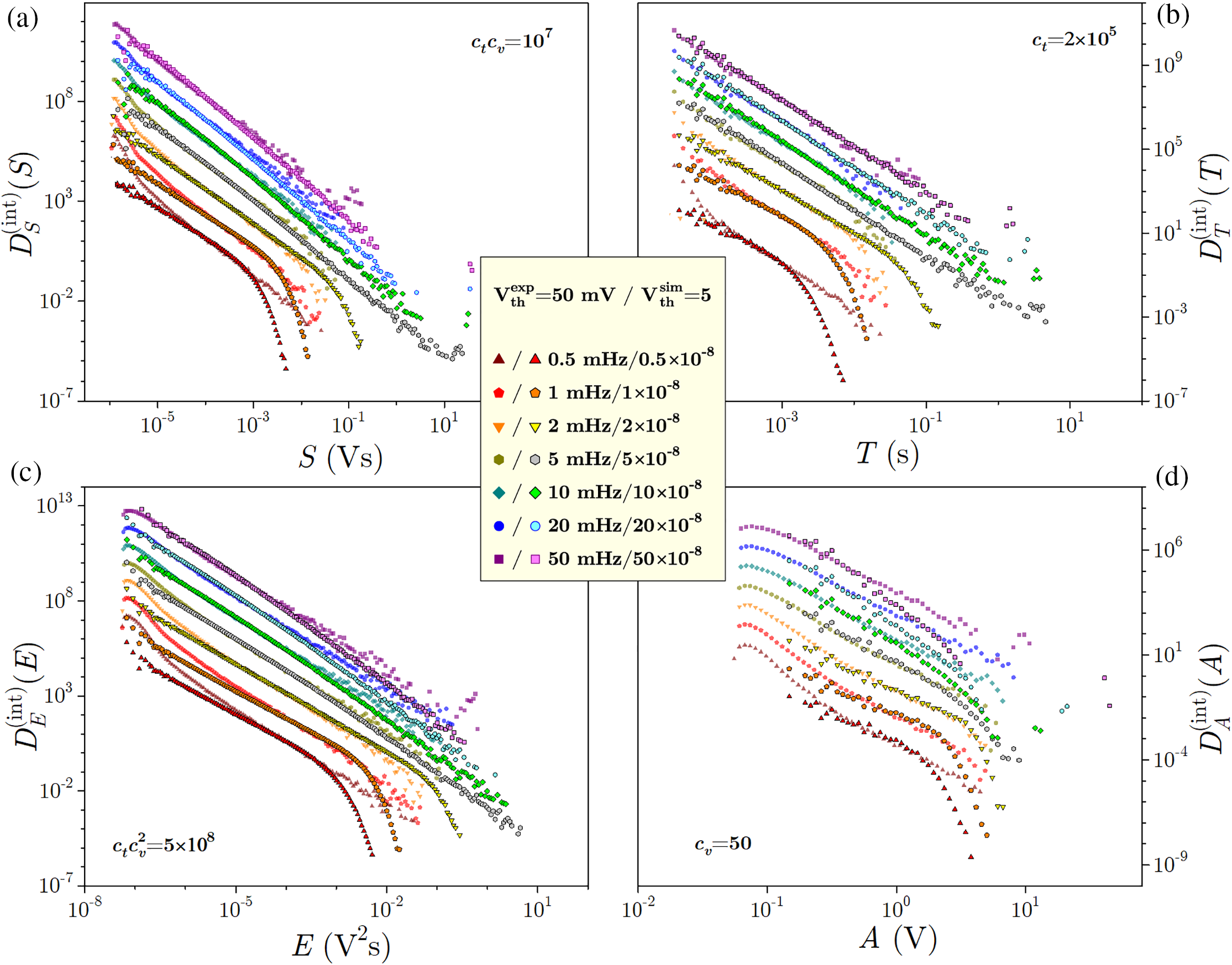
Figure 45: Comparison of integrated (unit area) distributions of avalanche parameters, size S in (a), duration T in (b), energy E in (c), and amplitude A in (d), obtained in experiments and numerical RFIM simulations on the
Further matching supporting the preceding conclusion is illustrated in Fig. 46, in the case of correlations
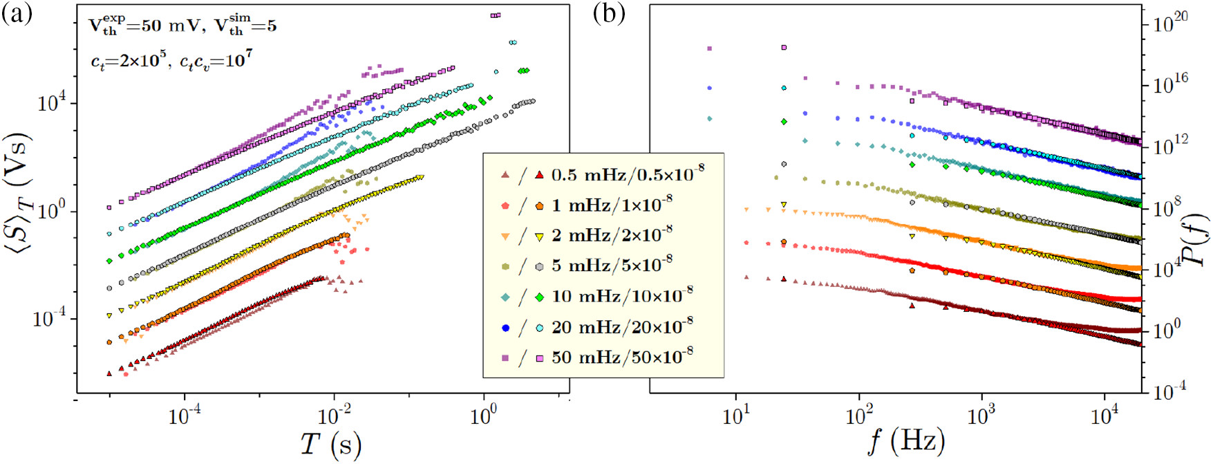
Figure 46: (a) Experimental and simulational correlations between the avalanche duration T and the average avalanche size
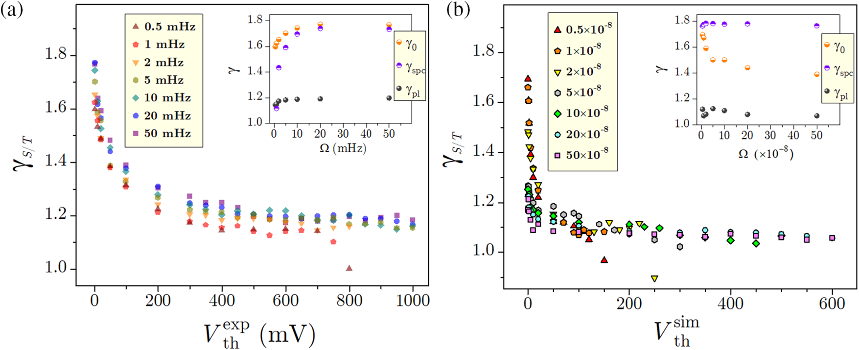
Figure 47: (a) Effective experimental values of the exponent
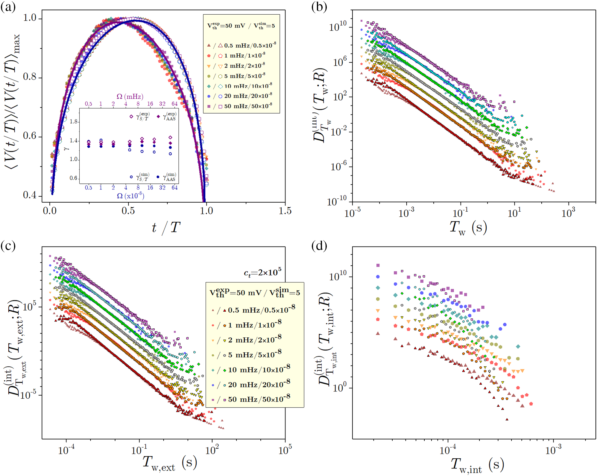
Figure 48: (a) Experimental/simulational average avalanche shapes shown in the main panel by filled/empty symbols and the values of exponents
7.2 Multifractal Analysis of BHN Reveals Impact of Relevant Parameters
The multifractality of time series manifests in nontrivial scaling properties of the generalized fluctuation function
is determined at each interval for
for
where the parameter
The scale-invariant segments of
where
Using a couple of representative examples, we demonstrate how the multifractal features of the BHN vary with the pertinent parameters and thus quantify their relevance to the magnetization reversal processes. As stated above, the multifractal features of BHN are tightly related to the collective (avalanching) magnetization fluctuations that also manifest in the long-range temporal correlations; they are often seen in the region of high-frequencies
The collective dynamic behavior in the BHN signals is not just a concept but a quantifiable reality. We further solidify this understanding by considering the temporal sequence of distinct avalanches. For example, the difference in the size of two consecutive avalanches
that universally appear in different complex dynamical systems out of equilibrium [202], where
7.2.1 Multifractality of BHN Varies with Demagnetizing Effects
As an interesting example, we analyze the structure of BHN signals simulated at low temperatures and varied demagnetizing factors by the extended RFIM (excluding the dipolar interactions term) in Eq. (1). For this purpose, we consider quasistatic driving, where the field increases for a given amount after an avalanche has stopped. It allows us to identify the impact of the propagation of individual avalanches on the magnetization fluctuations. We refer to Section 4.1 for more details on the quasistatic driving and Section 6 for the impact of demagnetizing fields on the shape of the hysteresis loop.
As stated above, the presence of demagnetizing fields induces long-range interactions counteracting the external magnetic field; they affect the shape of the hysteresis loop, in particular, introducing the extended linear segment in the central part of the loop, and potentially change the nature of critical behaviour; see Fig. 41. The magnetization reversal process is prolonged compared with the case without the demagnetizing fields (
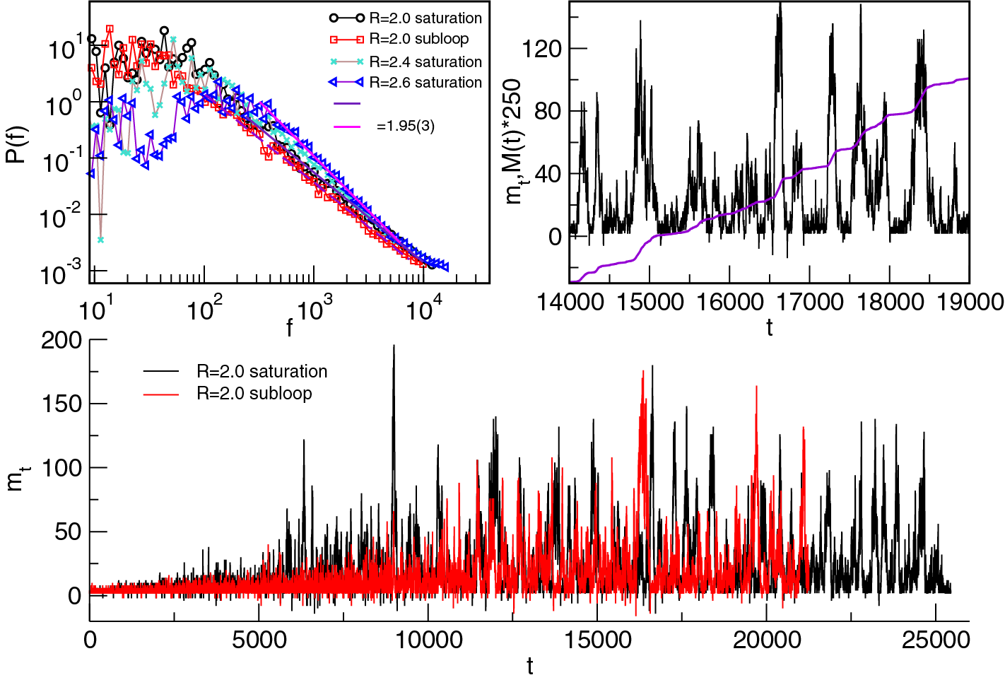
Figure 49: The bottom panel shows the magnetization fluctuations
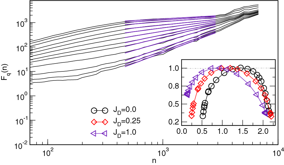
Figure 50: The fluctuation function
The fluctuation function
Considering a more realistic scenario, as explained above in Section 6 with the finite driving rates and thermal fluctuations, the structure of BHN was also analyzed in [164]. At very low relative temperatures and decisive demagnetizing factor
7.2.2 Multifractal BHN Spectra Vary with the System’s Spatial Dimension
Without demagnetizing fields,
Behavior in the central part of the loop is often monitored as closely related to the hysteresis-loop critical point [28,108]. The following example demonstrates the change of the hysteresis-loop critical behavior with the system’s dimensionality and its crucial impact on multifractal spectra. In samples with varied thickness, see a detailed study in [111], the critical disorder line
Considering the fluctuations
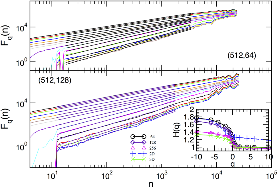
Figure 51: The fluctuation function
7.2.3 Other Factors That Influence the Structure of BHN at Low Temperatures
Besides the system’s dimensionality, which determines the universality class of critical behavior, and the strength of disorder (relative to the critical disorder point), which translates to the typical size of domains or the strength of the domain-walls pinning, the structure of BHN in disordered ferromagnets without demagnetizing fields exhibits characteristic variations depending on the considered segment of the hysteresis loop, driving rates and the potential presence of nonmagnetic defects. For demonstration, Fig. 52 shows some representative data, replotted from [33]. In the right panel, plots of the generalized Hurst exponents
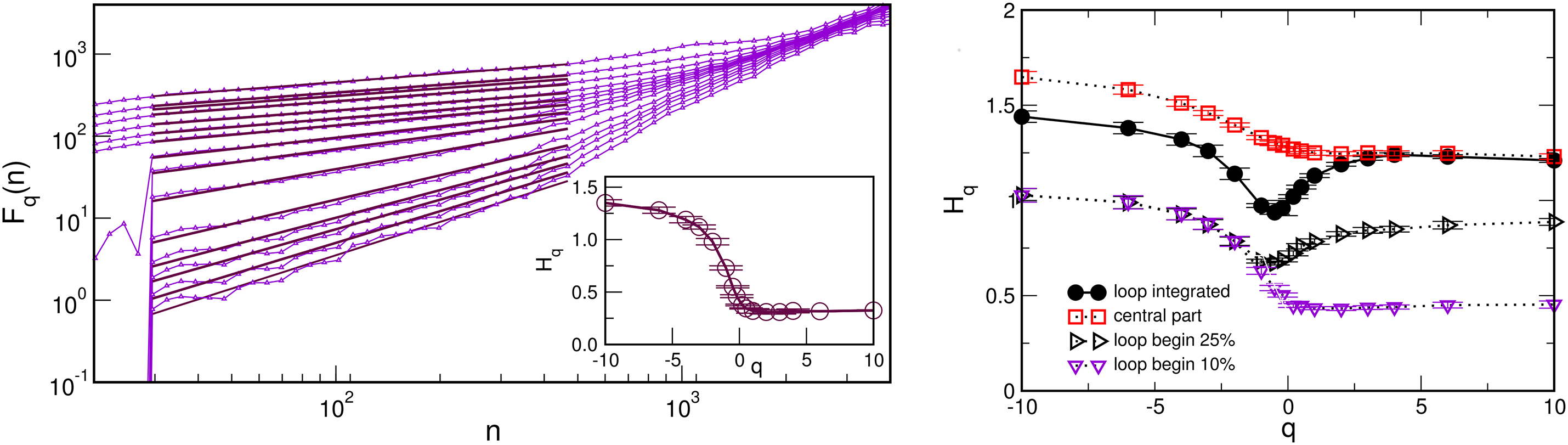
Figure 52: The left panel shows the fluctuation function
As stated above, the structure of the BHN is also sensitive to the driving rate. In particular, the increased driving rate leading to the spatio-temporal merging of the avalanches also results in the increased size of magnetization fluctuations; consequently, the whole reversal process is accomplished faster, resulting in a shorter time series overall. It manifests in the altered avalanche statistics, as discussed in Section 5. Increasing the driving rates also changes the multifractal properties of BHN, as shown in [33]. Specifically, the part of the spectrum corresponding to
The hysteretic response to the slow field ramping, which results in the collective magnetization fluctuations, also manifests in the structure of avalanche sequences. As stated above, the difference between the size of two consecutive avalanches is not a normal Gaussian; it exhibits a structure which is described by Tsallis distribution in Eq. (60). In Fig. 53, we show two examples of avalanche sequences, demonstrating that the non-extensivity parameter
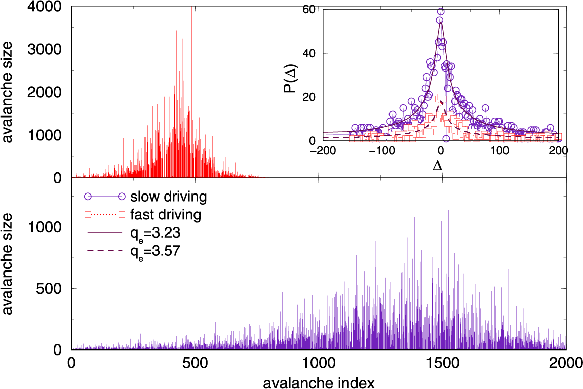
Figure 53: The bottom and top-left panels show the avalanche sequences for slow (
8 Response Signal Analysis with the Aid of Threshold
Being superposed on the magnetic response, thermal fluctuations prevent the decomposition of the response signal of the thermal RFIM systems into events that can be considered as essentially caused by magnetic interactions and only randomized by thermal noise. This is also the case for real (magnetic) systems where, besides thermal, some amount of noise of other origins appears (e.g., digital noise and/or noise caused by electromagnetic interference). In such cases, the decomposition of the response signal into (subsequently analyzed) events is accomplished with the use of threshold
The threshold value is not given in advance but instead has to be suitably chosen (e.g., estimated from the parts of the response signal in which the magnetic response could be rightly considered to be absent). Fortunately, in all situations with reasonably small/moderate overall noise, there is some range of not-too-small and too-big values of threshold such that for any
In this section, we show how the choice of threshold influences the statistics of the adiabatically driven ZT NEQ RFIM of homogeneous ferromagnetic spin systems (
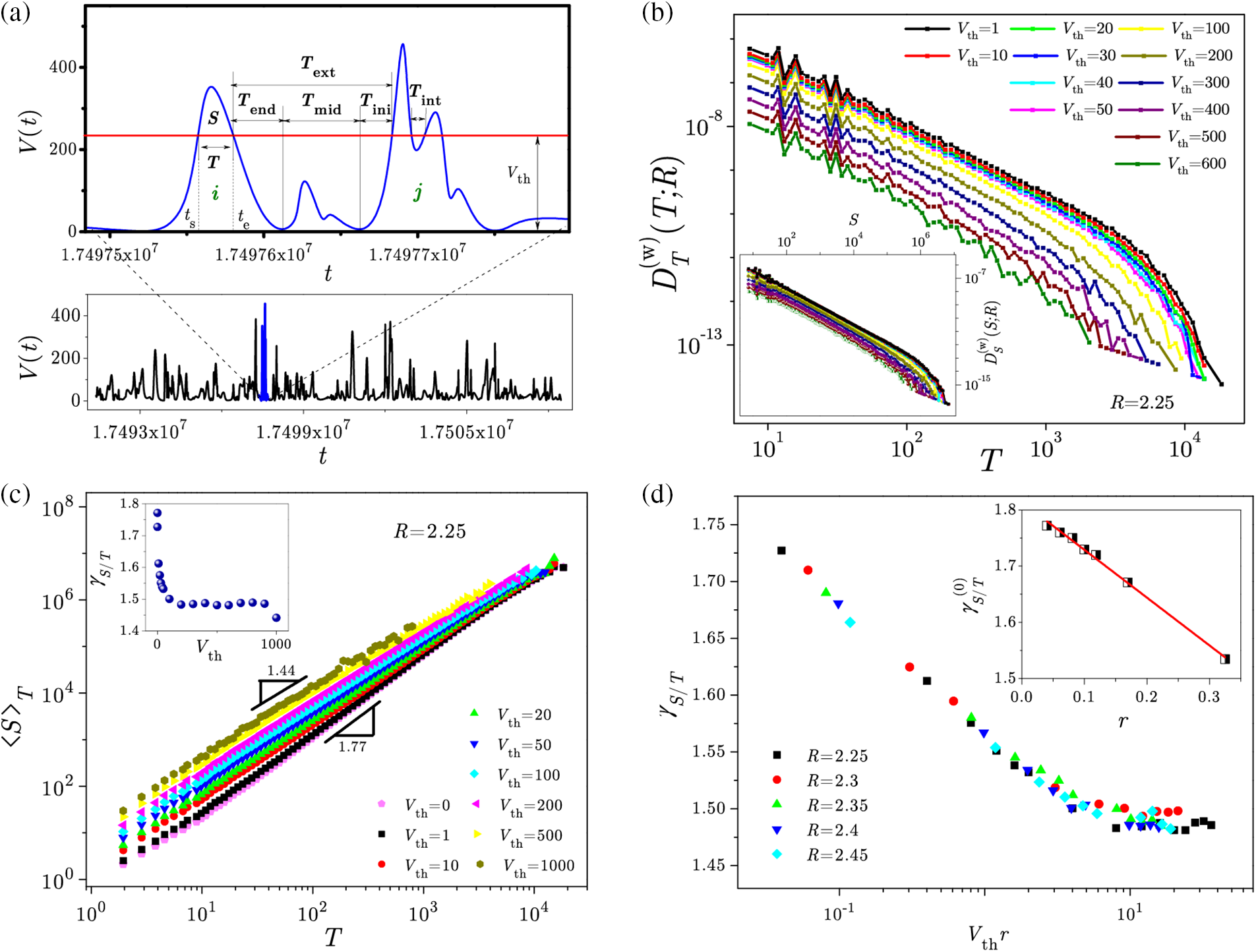
Figure 54: (a) Decomposition into events (i.e., subavalanches) of the response signal. For a (blue) part of a train of avalanches (shown in the bottom, and zoomed in the top part of this panel) and the imposed threshold
The values of
Starting from the conjecture that the temporal shape of avalanches satisfies the scaling conditions that are given by Eqs. (2) and (12) from Reference [140], the RFIM analysis in question revealed that the integrated distributions of avalanche duration,
provided that the conformity conditions
are satisfied. The same type of scaling is satisfied also for the windowed type of distributions, see Fig. 55 replotted from Fig. 3 of Reference [140].
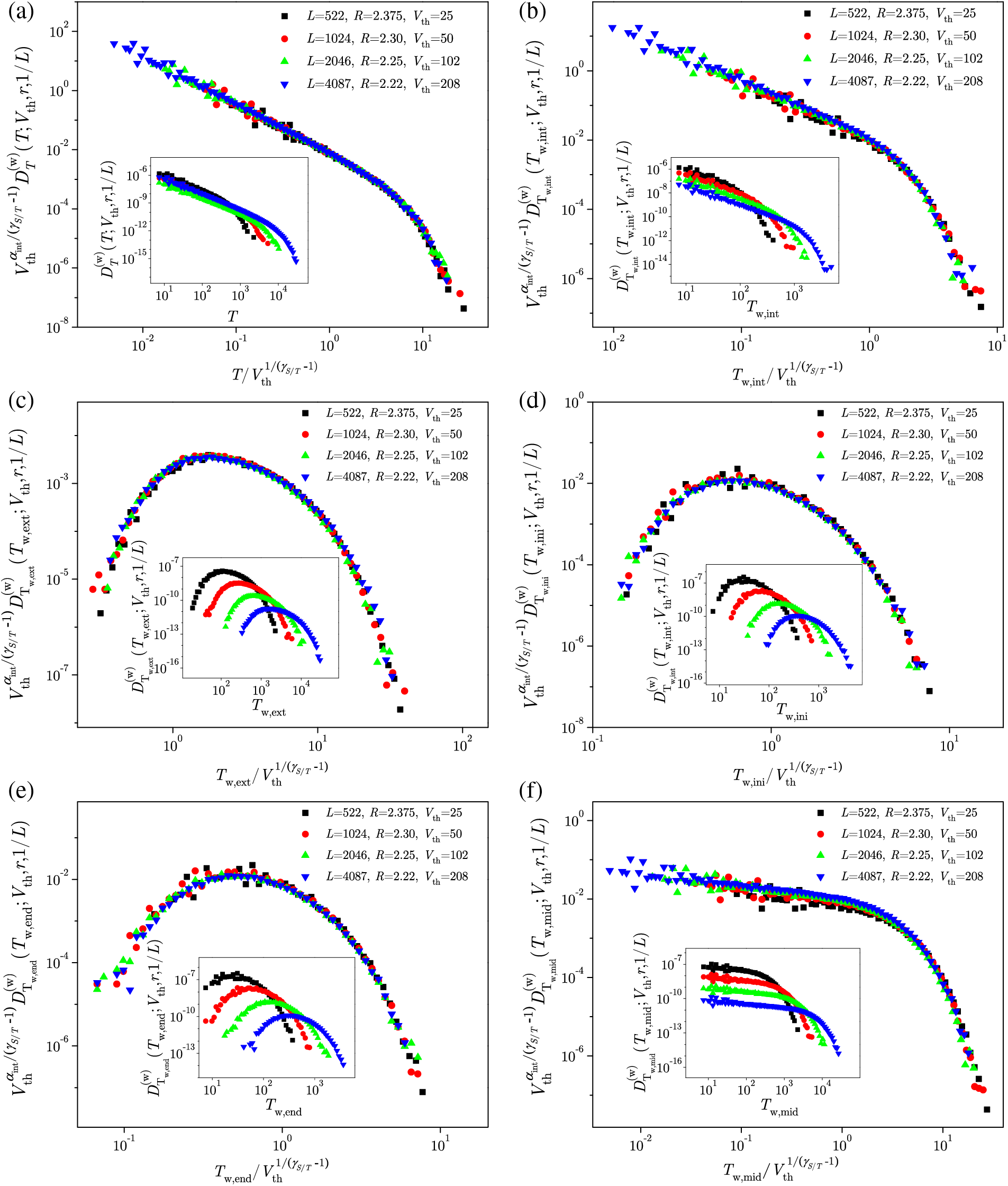
Figure 55: Collapsing of windowed distribution of duration and waiting time for the events (i.e., parts of the signal that are above threshold
The previous results are extended in the analysis [141] of the impact of the (zero-mean) noise added on the response signal manifesting only intrinsic thermal noise; see also [208]. The added noise is much greater than the system’s noise so that it only affects the registered signal and not the system dynamics. Such RFIM modification mimics the real systems influenced by the external noise originated from detectors, amplifiers, analog-to-digital (AD) converters, ambient electromagnetic interference (EMI), etc.
In Figs. 56 and 57 we illustrate the effect of added noise for the case of uniform white noise (UWN), i.e., the noise with standard deviation
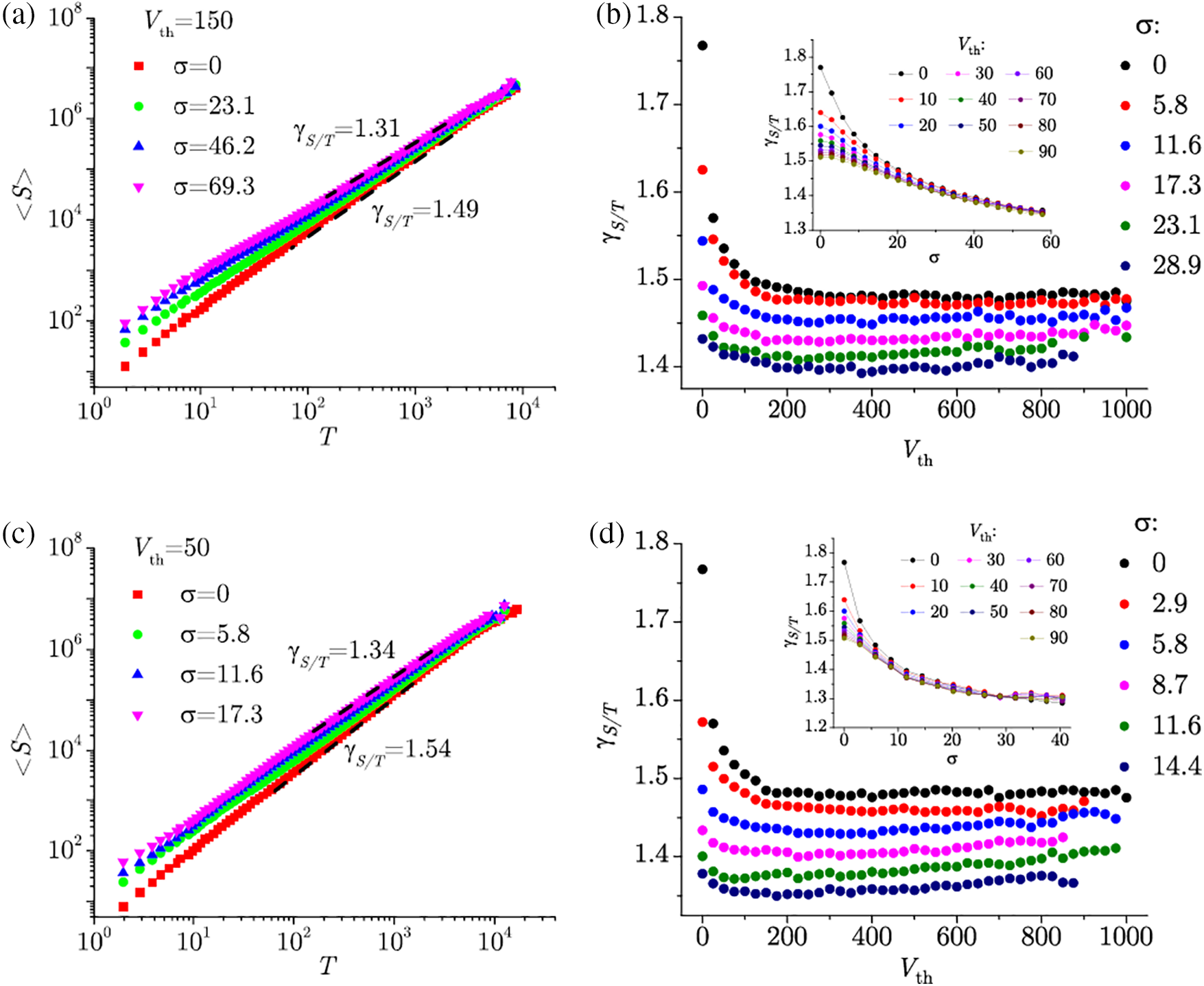
Figure 56: In this figure, combined are Figs. 2 and 4 from [141]: Left panels (a) and (c) show the average size
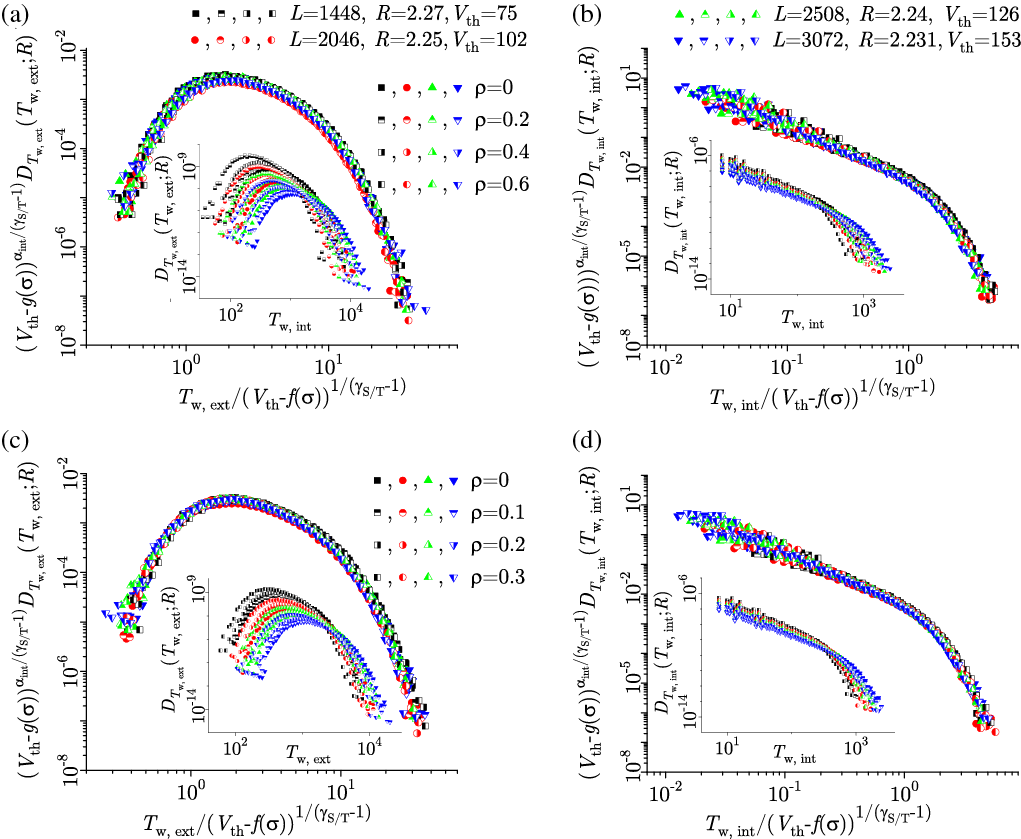
Figure 57: This is Fig. 13 from [141]. Graphs in main panels show the collapsing of the distributions of external waiting times (left column, (a) and (c) panels) and internal waiting times (right column, (b) and (d) panels) in the UWN case (top row, (a) and (b) panels) and GWN case (bottom row, (c) and (d) panels). These graphs correspond to the following four simulation parameters combinations
The impact of added noise is also noticeable in the power spectrum, average avalanche shapes, and all distributions of avalanche parameters. Nevertheless, the impact is most pronounced in the distributions of various types of waiting time (e.g., external and internal), as is evidenced in Fig. 57.
9 Summary, Limitations and Future Work
Supported by the presented works, one can identify two significant computational approaches. Specifically, we distinguish the theoretical limit of adiabatically driven systems with zero-temperature critical dynamics on one side, and the critical dynamics under the influence of a myriad of interrelated factors, i.e., the temperature, demagnetizing fields, and finite driving rates, resembling experimental situations, on the other.
The simplicity of employing Ising spins as binary variables, enables efficient simulations of the adiabatically driven systems, tailored in the sorted-list and the bit-per-spin algorithms. By these (and related) algorithms, the efficiency of the originally proposed codes for numerical simulations has been greatly improved, especially regarding the execution time and memory resources, which in large-scale system studies pose a significant computational load and an actual challenge. The implemented code enhancements made it possible to perform large-scale simulations of systems having up to more than
Streamlining the analysis, the systems being studied are regarded as ferromagnetic insulators, with magnetic walls indirectly defined as boundaries of cluster of spins with same orientation. The extended version of model allows for taking into consideration variable exchange couplings and anisotropy, and is open for inclusion of other types of magnetic interactions and external electromagnetic interference (EMI). It also enables the simulations of single and multilayered ferro/antiferromagnetic systems, accounting for lattice imperfections caused by vacancies and interstices, as well as simulations of amorphous systems. One of the limitations of the existing version of the model is that it does not consider the magneto-mechanical coupling, which leaves room for future development.
The relevance of conducted simulations is also verified quantitatively in comparison with the experimental data obtained in measurements of BHN. Used in numerous applications (e.g., as memory materials, thin films and nanowires), the disordered ferromagnetic materials are currently the subject of intensive ongoing research. In a complementary reciprocity, reliable and comprehensive experimental data is necessary for the development of adequate modeling tools, while simulation results can also serve as cornerstones and guidelines for experiments, calling for mutual advancements both in experimental techniques and optimizations of the employed algorithms. Beyond producing simulation results with practical applications, the future advancement might go along the lines of creating a more sophisticated and universal design technique, possibly applicable to other complex systems that exhibit an avalanche-like evolution, particularly those that like earthquakes could cause severe catastrophic consequences.
This article reviewed the developments and continuous progress in numerical modeling of the NEQ RFIM complementing the renormalization group theoretical investigations of out-of-equilibrium critical dynamics [37]. The preceding outlines highlight some of the potential difficulties and prospective avenues in this area of study, aiming to inspire motivation for future research and opportunities for further development. The corresponding main messages and some open questions are summarized below.
•
•
Adding demagnetizing fields in the Hamiltonian induces a specific type of long-range interactions that counteract the driving field; they change the shape of the hysteresis loop and the properties of the BHN signal. These effects increase with the strength of the demagnetizing factor
Among other open questions that remain for future work, we mention the demagnetizing effects in experimentally accessible antiferromagnetic-ferromagnetic bilayers, and the role of random fields in the hysteresis loop behaviour of antiferromagnetic materials and spin glasses (where the random field variance R appears as a field conjugate to a spin-glass order parameter). Furthermore, understanding the impact of more complex geometries, e.g., those that appear at a nanoscale suitably represented by nanonetworks, on spin ordering under the driving fields is a question of high interest due to the increasing use of the magnetic properties of nanoassemblies in modern technology applications. Theoretically, complex architectures of these assemblies support higher-order interactions; in conjunction with antiferromagnetic interactions among Ising spins, the topology of these assemblies appears as a decisive factor that shapes the hysteresis loop, thus altering the role of disorder as it is known in crystalline structures.
This review focuses on the hysteresis-loop criticality as a remarkable example of the out-of-equilibrium critical dynamics occurring during the magnetization reversal driven by the external field in disordered ferromagnetic materials. With the use of the nonequilibrium Random Field Ising Model as a paradigmatic model for theoretical investigations of disordered ferromagnets, we provide a comprehensive survey of mathematical modelling approaches to the simulations of spin-reversal processes for a variety of physical parameters and conditions motivated by theoretical requirements as well as the experimentally realizable situations. Concerning this matter, we present advanced computational techniques that are not just theoretical but also practical. By the results of several recent studies, we demonstrated the gain they led to in acquiring new physical insights into studied complex dynamical phenomena manifesting inherent scale invariance, finitesize scaling of the avalanche distributions, and the multifractal nature of the magnetization fluctuations in the Barkhausen nose time series near the disorder-induced critical point subject to additional physical parameters. The presented computational techniques utilizing the inherent scale-invariance of the hysteresis-loop criticality provide a deeper insight into magnetization reversal processes in disordered ferromagnetic systems, complementing the theoretical and experimental research. These powerful numerical methods can be adapted to study out-of-equilibrium dynamics in many-body quantum systems and other complex systems exhibiting nonequilibrium critical dynamics across the scales.
Acknowledgement: The authors are grateful to the journal editors for the invitation to write this review paper. The authors express their gratitude for the computing facilities provided by the Faculty of Physics in Belgrade, the Faculty of Science in Kragujevac, and the Scientific Computing Laboratory of the Institute of Physics in Belgrade. Having access to these high-performance computer clusters was essential to successfully carry out extensive numerical work in preparing the (here reviewed) authors’ papers which greatly influenced the results and conclusions this study overviews.
Funding Statement: Djordje Spasojević and Svetislav Mijatović acknowledge the support from the Ministry of Science, Technological Development and Innovation of the Republic of Serbia (Agreement No. 451-03-65/2024-03/200162), S.J. ibid. (Agreement No. 451-03-65/2024-03/200122), and Bosiljka Tadić from the Slovenian Research Agency (program P1-0044).
Author Contributions: The authors confirm contribution to the paper as follows. Regarding the review article: conception and design: Djordje Spasojević, Sanja Janićević, Svetislav Mijatović and Bosiljka Tadić; draft manuscript preparation: Djordje Spasojević, Sanja Janićević and Bosiljka Tadić. Regarding the author’s original papers: software preparation: Djordje Spasojević and Bosiljka Tadić; data collection: Sanja Janićević and Svetislav Mijatović; analysis and interpretation of results: Djordje Spasojević, Sanja Janićević, Svetislav Mijatović and Bosiljka Tadić. All authors reviewed the results and approved the final version of the manuscript.
Availability of Data and Materials: All of the data from the authors’ published studies presented in this review article are available upon reasonable request.
Ethics Approval: Not applicable.
Conflicts of Interest: The authors declare no conflicts of interest to report regarding the present study.
References
1. Honkanen M, Lukinmaa H, Kaappa S, Santa-aho S, Kajan J, Savolainen S, et al. Magnetic domain wall dynamics studied by in-situ Lorentz microscopy with aid of custom-made Hall effect sensor holder. Ultramicroscopy. 2024;262:113979. doi:10.1016/j.ultramic.2024.113979. [Google Scholar] [PubMed] [CrossRef]
2. Santa-aho S, Honkanen M, Kaappa S, Azzari R, Saren A, Ullakko K, et al. Multi-instrumental approach to domain walls and their movement in ferromagnetic steels-origin of barkhausen noise studied by microscopy techniques. Mater Des. 2023;234(1):112308. doi:10.1016/j.matdes.2023.112308. [Google Scholar] [CrossRef]
3. Honkanen M, Santa-aho S, Laurson L, Eslahi N, Foi A, Vippola M. Mimicking Barkhausen noise measurement by in-situ transmission electron microscopy-effect of microstructural steel features on Barkhausen noise. Acta Mater. 2021;221:117378. doi:10.1016/j.actamat.2021.117378. [Google Scholar] [CrossRef]
4. Papavasileiou AV, Menelaou M, Sarkar KJ, Sofer Z, Polavarapu L, Mourdikoudis S. Ferromagnetic elements in two-dimensional materials: 2D magnets and beyond. Adv Funct Mater. 2023;34(2):2309046. doi:10.1002/adfm.202309046. [Google Scholar] [CrossRef]
5. Liang X, Dong C, Chen H, Wang J, Wei Y, Zaeimbashi M, et al. A review of thin-film magnetoelastic materials for magnetoelectric applications. Sensors. 2020;20(5):1532. doi:10.3390/s20051532. [Google Scholar] [PubMed] [CrossRef]
6. Rasaili P, Sharma NK, Bhattarai A. Comparison of ferromagnetic materials: past work, recent trends, and applications. Condens Matter. 2022;7(1):12. doi:10.3390/condmat7010012. [Google Scholar] [CrossRef]
7. Yao Y, Zhan X, Sendeku MG, Yu P, Dajan FT, Zhu C, et al. Recent progress on emergent two-dimensional magnets and heterostructures. Nanotechnology. 2021;32:472001. [Google Scholar]
8. Bertotti G. Hysteresis in magnetism. Boston: Academic Press; 1998. [Google Scholar]
9. Bertotti G, Mayergoyz ID. The science of hysteresis, vol. II: physical modeling, micromagnetics, and magnetization dynamics. Amsterdam: Academic Press; 2006. [Google Scholar]
10. Li P, Zhang J, Gao Y, Xia X, Weng GJ. Effect of magnetic field on macroscopic hysteresis and microscopic magnetic domains for different ferromagnetic materials. J Mater Res Technol. 2024;31:458–71. [Google Scholar]
11. Balakrishna AR. Rethinking hysteresis in magnetic materials. MRS Commun. 2024;14:835–45. doi:10.1557/s43579-024-00624-6. [Google Scholar] [CrossRef]
12. Kovacs A, Exl L, Kornell A, Fischbacher J, Hovorka M, Gusenbauer M, et al. Image-based prediction and optimization of hysteresis properties of nanocrystalline permanent magnets using deep learning. J Magn Magn Mater. 2024;596:171937. doi:10.1016/j.jmmm.2024.171937. [Google Scholar] [CrossRef]
13. Schwarz A, Liebmann M, Kaiser U, Wiesendanger R, Noh TW, Kim DW. Visualization of the Barkhausen effect by magnetic force microscopy. Phys Rev Lett. 2004;92:077206. [Google Scholar] [PubMed]
14. Alessandro B, Beatrice C, Bertotti G, Montorsi A. Domain wall dynamics and Barkhausen effect in metallic ferromagnetic materials. J Appl Phys. 1990;68:2901. [Google Scholar]
15. Bertotti G, Durin G, Magni A. Scaling aspects of domain wall dynamics and Barkhausen effect in ferromagnetic materials. J Appl Phys. 1994;75:5490. [Google Scholar]
16. Durin G, Magni A, Bertotti G. Measurements of the Barkhausen effect in FeCoB amorphous alloys. J Magnet Magnet Mater. 1996;160:299–301. [Google Scholar]
17. Spasojević D, Bukvić S, Milošević S, Stanley HE. Barkhausen noise: elementary signals, power laws, and scaling relations. Phys Rev E. 1996;54:2531. [Google Scholar]
18. Lee WY, Choi BC, Xu YB, Bland JAC. Magnetization reversal dynamics in epitaxial Fe/GaAs(001) thin films. Phys Rev B. 1999;60(14):10216. doi:10.1103/PhysRevB.60.10216. [Google Scholar] [CrossRef]
19. Moore TA, Rothman J, Xu YB, Bland JAC. Thickness-dependent dynamic hysteresis scaling behavior in epitaxial Fe/GaAs(001) and Fe/InAs(001) ultrathin films. J Appl Phys. 2001;89(11):7018. doi:10.1063/1.1357840. [Google Scholar] [CrossRef]
20. Ryu KS, Akinaga H, Shin SC. Tunable scaling behaviour observed in Barkhausen criticality of a ferromagnetic film. Nature Phys. 2007;3(8):547–50. doi:10.1038/nphys659. [Google Scholar] [CrossRef]
21. Estévez V, Laurson L. Magnetic domain-wall dynamics in wide permalloy strips. Phys Rev B. 2016;93(6):064403. doi:10.1103/PhysRevB.93.064403. [Google Scholar] [CrossRef]
22. Dos Santos Lima GZ, Corso G, Correa MA, Sommer RL, Ivanov PC, Bohn F. Universal temporal characteristics and vanishing of multifractality in Barkhausen avalanches. Phys Rev E. 2017;96(2):022159. doi:10.1103/PhysRevE.96.022159. [Google Scholar] [CrossRef]
23. Lee HS, Ryu KS, Jeon KR, Parkin SSP, Shin SC. Breakdown of Barkhausen critical-scaling behavior with increasing domain-wall pinning in ferromagnetic films. Phys Rev B Condens Matt Mater Phy. 2011;83(6):060410. doi:10.1103/PhysRevB.83.060410. [Google Scholar] [CrossRef]
24. Krasnytska M, Berche B, Holovatch Y, Kenna R. Ising model with variable spin/agent strengths. J Phy: Comp. 2020;1(3):035008. doi:10.1088/2632-072X/abb654. [Google Scholar] [CrossRef]
25. Vives E, Planes A. Avalanches in a fluctuationless first-order phase transition in a random-bond Ising model. Phys Rev B. 1994;50(6):3839–48. doi:10.1103/PhysRevB.50.3839. [Google Scholar] [CrossRef]
26. Tadić B. Nonuniversal scaling behavior of Barkhausen noise. Phys Rev Lett. 1996;77(18):3843. doi:10.1103/PhysRevLett.77.3843. [Google Scholar] [PubMed] [CrossRef]
27. Pérez-Reche FJ, Vives E. Finite-size scaling analysis of the avalanches in the three-dimensional Gaussian random-field Ising model with metastable dynamics. Phys Rev B. 2003;67(13):134421. doi:10.1103/PhysRevB.67.134421. [Google Scholar] [CrossRef]
28. Sethna JP, Dahmen KA, Perković O. Random-field Ising models of hysteresis edited by Bertotti G and Mayergoyz I. Sci Hysteres. 2006;2:107–79. [Google Scholar]
29. Zapperi S, Cizeau P, Durin G, Stanley HE. Dynamics of a ferromagnetic domain wall: avalanches, depinning transition, and the Barkhausen effect. Phys Rev B. 1998;58:6353. [Google Scholar]
30. Tadić B. Dynamic criticality in driven disordered systems: role of depinning and driving rate in Barkhausen noise. Phys A: Statist Mech Appl. 1999;270:125–34. [Google Scholar]
31. Perković O, Dahmen KA, Sethna JP. Disorder-induced critical phenomena in hysteresis: numerical scaling in three and higher dimensions. Phys Rev B. 1999;59:6106. [Google Scholar]
32. Vives E, Planes A. Hysteresis and avalanches in disordered systems. J Magnet Magnet Mater. 2000;221:164–71. [Google Scholar]
33. Tadić B. Multifractal analysis of Barkhausen noise reveals the dynamic nature of criticality at hysteresis loop. J Statist Mech. 2016;6:063305. [Google Scholar]
34. Belanger DP, Nattermann T. Spin glasses and random fields edited by Young A. P. Series Direct Condens Matter Phys. 1998;12:251–98. [Google Scholar]
35. Dahmen KA, Sethna JP. Hysteresis loop critical exponents in
36. Fytas NG, Martin-Mayor V, Picco M, Sourlas N. Phase transitions in disordered systems: The example of the random-field Ising model in four dimensions. Phys Rev Lett. 2016;16:227201. [Google Scholar]
37. Balog I, Tarjus G, Tissier M. Criticality of the random field Ising model in and out of equilibrium: a nonperturbative functional renormalization group description. Phys Rev B. 2018;97:094204. [Google Scholar]
38. Cardy J. Random-field effects in site-disordered Ising antiferromagnets. Phys Rev B. 1984;29:505. [Google Scholar]
39. Fishman S, Aharony A. Random field effects in disordered anisotropic antiferromagnets. J Phys C: Solid State Phys. 1979;12:L729. [Google Scholar]
40. Joshi DC, Nordblad P, Mathieu R. Random fields and apparent exchange bias in the dilute Ising antiferromagnet Fe0.6Zn0.4F2. Sci Rep. 2020;10:14588. [Google Scholar] [PubMed]
41. Ghara S, Barts E, Vasin K, Kamenskyi D, Prodan L, Tsurkan V, et al. Magnetization reversal through an antiferromagnetic state. Nat Commun. 2023;14:5174. [Google Scholar] [PubMed]
42. Semenov YG, Wook Kim K. Modeling of antiferromagnetic dynamics: a brief review. IEEE Nanotechnol Mag. 2020;14:32. [Google Scholar]
43. Chen H, Liu L, Zhou X, Meng Z, Wang X, Duan Z, et al. Emerging antiferromagnets for spintronics. Adv Mater Deerfield. 2024;36:2310379. [Google Scholar]
44. Khatua J, Pregelj M, Elghandour A, Jagličic Z, Klingeler R, Zorko A, et al. Magnetic properties of the triangular-lattice antiferromagnets Ba3RB9O18 (R = Yb, Er). Phys Rev B. 2022;106:104408. [Google Scholar]
45. EPJ B. Topical issue: 100 glorious years of the Ising model. Eur Phys J B. 2024. [Google Scholar]
46. Durin G, Zapperi S. Random-field Ising models of hysteresis. In: Bertotti G, Mayergoyz I, editors. The science of hysteresis, vol. II: physical modeling, micromagnetics, and magnetization dynamics. Amsterdam: Academic Press; 2006. p. 181–267. [Google Scholar]
47. Hristopulos DT. Random fields for spatial data modeling-a primer for scientists and engineers. Springer Netherlands: Springer Dordrecht; 2020. [Google Scholar]
48. Sethna JP, Dahmen KA, Kartha S, Krumhansl JA, Roberts BW, Shore JD. Hysteresis and hierarchies: dynamics of disorder-driven first-order phase transformations. Phys Rev Lett. 1993;70:3347. [Google Scholar] [PubMed]
49. Uhl JT, Pathak S, Schorlemmer D, Liu X, Swindeman R, Brinkman BAW, et al. Universal quake statistics: from compressed nanocrystals to earthquakes. Sci Rep. 2015;5(1):16493. [Google Scholar] [PubMed]
50. Omori F. On aftershocks of earthquakes. J Coll Sci Imper Univ Tokyo. 1894;7:111–200. [Google Scholar]
51. Jagla EA, Landes FP, Rosso A. Viscoelastic effects in avalanche dynamics: a key to earthquake statistics. Phys Rev Lett. 2014;112:174301. [Google Scholar] [PubMed]
52. Davidsen J, Baiesi M. Self-similar aftershock rates. Phys Rev E. 2016;94(2):022314. doi:10.1103/PhysRevE.94.022314. [Google Scholar] [PubMed] [CrossRef]
53. Bizzarri A, Petri A, Baldassarri A. Earthquake dynamics constrained from laboratory experiments: new insights from granular materials. Ann Geophys. 2021;64(4):SE441. doi:10.4401/ag-8613. [Google Scholar] [CrossRef]
54. Fisher DS. Collective transport in random media: from superconductors to earthquakes. Phys Rep. 1998;301(1–3):113. doi:10.1016/S0370-1573(98)00008-8. [Google Scholar] [CrossRef]
55. Laurson L, Santucci S, Zapperi S. Avalanches and clusters in planar crack front propagation. Phys Rev E. 2010;81(4):046116. doi:10.1103/PhysRevE.81.046116. [Google Scholar] [CrossRef]
56. Baró J, Corral A, Illa X, Planes A, Salje EKH, Schranz W, et al. Statistical similarity between the compression of a porous material and earthquakes. Phys Rev Lett. 2013;110(8):088702. doi:10.1103/PhysRevLett.110.088702. [Google Scholar] [CrossRef]
57. Savolainen J, Laurson L, Alava MJ. Effect of thresholding on avalanches and their clustering for interfaces with long-range elasticity. Phys Rev E. 2022;105:054152. [Google Scholar] [PubMed]
58. Salje EKH, Jiang X. Crackling noise and avalanches in minerals. Phys Chem Miner. 2021;48:22. [Google Scholar]
59. Lombardi F, Herrmann HJ, Plenz D, de Arcangelis L. Temporal correlations in neuronal avalanche occurrence. Sci Rep. 2016;6:24690. [Google Scholar] [PubMed]
60. Miller SR, Yu S, Plenz D. The scale-invariant, temporal profile of neuronal avalanches in relation to cortical
61. Friedman N, Ito S, Brinkman BAW, Shimono M, DeVille REL, Dahmen KA, et al. Universal critical dynamics in high resolution neuronal avalanche data. Phys Rev Lett. 2012;108:208102. [Google Scholar] [PubMed]
62. Bédard C, Kroger H, Destexhe A. Does the 1/f frequency scaling of brain signals reflect self-organized critical states? Phys Rev Lett. 2006;97:118102. doi:10.1103/PhysRevLett.97.118102. [Google Scholar] [PubMed] [CrossRef]
63. Alava MJ, Laurson L, Zapperi S. Crackling noise in plasticity. Eur Phys J Spec Top. 2014;223:2353–67. [Google Scholar]
64. Janićević S, Ovaska M, Alava MJ, Laurson L. Avalanches in 2D dislocation systems without applied stresses. J Statist Mech. 2015;2015:P07016. [Google Scholar]
65. Ispánovity PD, Ugi D, Péterffy G, Knapek M, Kalácska S, Tüzes D, et al. Dislocation avalanches are like earthquakes on the micron scale. Nat Commun. 2022;13:1975. [Google Scholar]
66. Ispánovity PD, Laurson L, Zeiser M, Groma I, Zapperi S, Alava MJ. Avalanches in 2D dislocation systems: plastic yielding is not depinning. Phys Rev Lett. 2014;112:235501. [Google Scholar]
67. Planet R, Santucci S, Zeiser M, Ortín J. Avalanches and non-gaussian fluctuations of the global velocity of imbibition fronts. Phys Rev Lett. 2009;102:094502. [Google Scholar] [PubMed]
68. Nataf GF, Castillo-Villa PO, Baró J, Illa X, Vives E, Planes A, et al. Avalanches in compressed porous SiO2-based materials. Phys Rev E. 2014;90:022405. doi:10.1103/PhysRevE.90.022405. [Google Scholar] [PubMed] [CrossRef]
69. Mäkinen T, Miksic A, Ovaska MJA. Avalanches in wood compression. Phys Rev Lett. 2015;115:055501. [Google Scholar]
70. Bouchaud JP. Crises and collective socio-economic phenomena: simple models and challenges. J Statist Phys. 2013;151:567–606. [Google Scholar]
71. Pinto OA, Muñoz MA. Quasi-neutral theory of epidemic outbreaks. PLoS One. 2011;6:e21946. [Google Scholar] [PubMed]
72. Mijatović S, Graovac S, Spasojević D, Tadić B. Tuneable hysteresis loop and multifractal oscillations of magnetisation in weakly disordered antiferromagnetic-ferromagnetic bilayers. Phys E: Low-Dimens Syst Nanostruct. 2022;142:115319. [Google Scholar]
73. Chen G, Collette D, Urazhdin S. Experimental demonstration and analysis of random field effects in ferromagnet/antiferromagnet bilayers. Phys Rev B. 2020;101:144427. [Google Scholar]
74. Liu S, Li MR, Zhang SX, Jian SK, Yao H. Universal Kardar-Parisi-Zhang scaling in noisy hybrid quantum circuits. Phys Rev B. 2023;107:L201113. [Google Scholar]
75. Ren J, Li Q, Li W, Cai Z, Wang X. Noise-driven universal dynamics towards an infinite temperature state. Phys Rev Lett. 2020;124:130602. [Google Scholar] [PubMed]
76. King AD, Raymond J, Lanting T, Harris R, Zucca A, Altomare F, et al. Quantum critical dynamics in a 5,000-qubit programmable spin glass. Nature. 2023;617:61–6. [Google Scholar] [PubMed]
77. Živković J, Tadić B. Nanonetworks: the graph theory framework for modeling nanoscale systems. Nanoscale Syst: Math Model, Theory Appl. 2013;2:30–48. [Google Scholar]
78. Tadić B, Melnik R. Fundamental interactions in self-organised critical dynamics on higher order networks. Eur Phys J B. 2024;97(6):68. doi:10.1140/epjb/s10051-024-00705-4. [Google Scholar] [CrossRef]
79. Adeyeye AO, Singh N. Large area patterned magnetic nanostructures. J Phys D: Appl Phys. 2008;41(15):153001. doi:10.1088/0022-3727/41/15/153001. [Google Scholar] [CrossRef]
80. Li J, Li G, Lu X, Wang S, Leng M, Yang S, et al. Magnetically responsive optical modulation: from anisotropic nanostructures to emerging applications. Adv Funct Mater. 2024;34(3):2308293. doi:10.1002/adfm.202308293. [Google Scholar] [CrossRef]
81. Tadić B, Andjelković M, Šuvakov M, Rodgers GJ. Magnetisation processes in geometrically frustrated spin networks with self-assembled cliques. Entropy. 2020;22(3):336. doi:10.3390/e22030336. [Google Scholar] [PubMed] [CrossRef]
82. Hang C, Liu W, Dobmann G, Wu Y, Chen W, Wang P. Ising model simulation and empirical research of Barkhausen noise. J Nondestruct Eval. 2024;43(1):20. doi:10.1007/s10921-023-01037-6. [Google Scholar] [CrossRef]
83. Mijatović S, Jovković D, Janićević S, Graovac S, Spasojević D. A tool for identifying the criticality in the disordered systems with metastable dynamics. Phys A: Statist Mech Appl. 2021;572:125883. [Google Scholar]
84. Dahmen KA, Sethna JP. Hysteresis, avalanches, and disorder-induced critical scaling: a renormalization-group approach. Phys Rev B. 1996;53:14872. [Google Scholar]
85. Spasojević D, Janićević S, Knežević M. Exact results for mean-field zero-temperature random-field Ising model. Europhys Lett. 2006;76:912. [Google Scholar]
86. Vives E, Rosinberg ML, Tarjus G. Hysteresis and avalanches in the T = 0 random-field Ising model with two-spin-flip dynamics. Phys Rev B. 2005;71:134424. [Google Scholar]
87. Liu Y, Dahmen KA. Random-field Ising model in and out of equilibrium. Europhys Lett. 2009;86:56003. [Google Scholar]
88. Liu Y, Dahmen KA. Unexpected universality in static and dynamic avalanches. Phys Rev E. 2009;79(6):061124. doi:10.1103/PhysRevE.79.061124. [Google Scholar] [CrossRef]
89. Spasojević D, Janićević S, Knežević M. Numerical evidence for critical behavior of the two-dimensional nonequilibrium zero-temperature random field Ising model. Phys Rev Lett. 2011;106(17):175701. doi:10.1103/PhysRevLett.106.175701. [Google Scholar] [PubMed] [CrossRef]
90. Spasojević D, Janićević S, Knežević M. Avalanche distributions in the two-dimensional nonequilibrium zero-temperature random field Ising model. Phys Rev E. 2011;84(5):051119. doi:10.1103/PhysRevE.84.051119. [Google Scholar] [CrossRef]
91. Aizenman M, Wehr J. Rounding of first-order phase transitions in systems with quenched disorder. Phys Rev Lett. 1989;62(21):2503. doi:10.1103/PhysRevLett.62.2503. [Google Scholar] [PubMed] [CrossRef]
92. Bricmont J, Kupiainen A. Lower critical dimension for the random-field Ising model. Phys Rev Lett. 1987;59(16):1829. doi:10.1103/PhysRevLett.59.1829. [Google Scholar] [PubMed] [CrossRef]
93. Southern BW, Young AP. Real space rescaling study of spin glass behaviour in three dimensions. J Phys C: Solid State Phys. 1977;10:2179. [Google Scholar]
94. Parisi G, Sourlas N. Random magnetic fields, supersymmetry, and negative dimensions. Phys Rev Lett. 1979;43:744. [Google Scholar]
95. Parisi G, Sourlas N. Scale invariance in disordered systems: the example of the random-field Ising model. Phys Rev Lett. 2002;89:257204. [Google Scholar] [PubMed]
96. Tissier M, Tarjus G. Supersymmetry and its spontaneous breaking in the random field Ising model. Phys Rev Lett. 2011;107:041601. [Google Scholar] [PubMed]
97. Fytas NG, Martin-Mayor V. Universality in the three-dimensional random-field Ising model. Phys Rev Lett. 2013;110:227201. [Google Scholar] [PubMed]
98. Fytas NG, Martin-Mayor V, Picco M, Sourlas N. Restoration of dimensional reduction in the random-field Ising model at five dimensions. Phys Rev E. 2017;95:042117. [Google Scholar] [PubMed]
99. Fytas NG, Martin-Mayor V, Parisi G, Picco M, Sourlas N. Evidence for supersymmetry in the random-field Ising model at d = 5. Phys Rev Lett. 2019;122:240603. [Google Scholar] [PubMed]
100. Janićević S, Mijatović S, Spasojević D. Critical behavior of the two-dimensional nonequilibrium zero-temperature random field Ising model on a triangular lattice. Phys Rev E. 2017;95:042131. [Google Scholar] [PubMed]
101. Tadić B. Dynamical implications of sample shape for avalanches in 2-dimensional random-field Ising model with saw-tooth domain wall. Phys A: Statist Mech Appl. 2018;493:330–41. [Google Scholar]
102. Kurbah L, Thongjaomayum D, Shukla P. Nonequilibrium random-field Ising model on a diluted triangular lattice. Phys Rev E. 2015;91:012131. [Google Scholar]
103. Mijatović S, Jovković D, Spasojević D. Nonequilibrium athermal random-field Ising model on hexagonal lattices. Phys Rev E. 2021;103:032147. [Google Scholar] [PubMed]
104. Chen YJ, Papanikolau S, Sethna JP, Zapperi S, Durin G. Avalanche spatial structure and multivariable scaling functions: sizes, heights, widths, and views through windows. Phys Rev E. 2011;84:061103. [Google Scholar]
105. Brinkman BAW, Dahmen KA. Tuning coupling: discrete changes in runaway avalanche sizes in disordered media. Phys Rev E. 2011;84:041129. [Google Scholar]
106. Pérez-Reche FJ, Vives E. Spanning avalanches in the three-dimensional Gaussian random-field Ising model with metastable dynamics: field dependence and geometrical properties. Phys Rev B. 2004;70:214422. [Google Scholar]
107. Spasojević D, Janićević S, Knežević M. Analysis of spanning avalanches in the two-dimensional nonequilibrium zero-temperature random-field Ising model. Phys Rev E. 2014;89:012118. [Google Scholar]
108. Janićević S, Knežević D, Mijatović S, Spasojević D. Scaling domains in the nonequilibrium athermal random field Ising model of finite systems. J Statist Mech. 2021;2021(1):013202. doi:10.1088/1742-5468/abcd32. [Google Scholar] [CrossRef]
109. Navas-Portella V, Vives E. Influence of the aspect ratio and boundary conditions on universal finite-size scaling functions in the athermal metastable two-dimensional random field Ising model. Phys Rev E. 2016;93(2):022129. doi:10.1103/PhysRevE.93.022129. [Google Scholar] [PubMed] [CrossRef]
110. Spasojević D, Mijatović S, Navas-Portela V, Vives E. Crossover from three-dimensional to two-dimensional systems in the nonequilibrium zero-temperature random-field Ising model. Phys Rev E. 2018;97(1):012109. doi:10.1103/PhysRevE.97.012109. [Google Scholar] [PubMed] [CrossRef]
111. Tadić B, Mijatović S, Janićević S, Spasojević D, Rodgers GJ. The critical Barkhausen avalanches in thin random-field ferromagnets with an open boundary. Sci Rep. 2019;9(1):6349. doi:10.1038/s41598-019-42802-w. [Google Scholar] [CrossRef]
112. Mijatović S, Jovković D, Janićević S, Spasojević D. Critical disorder and critical magnetic field of the nonequilibrium athermal random-field Ising model in thin systems. Phys Rev E. 2019;100(3):032113. doi:10.1103/PhysRevE.100.032113. [Google Scholar] [PubMed] [CrossRef]
113. Laurson L, Durin G, Zapperi S. Universality classes and crossover scaling of Barkhausen noise in thin films. Phys Rev B. 2014;89(10):104402. doi:10.1103/PhysRevB.89.104402. [Google Scholar] [CrossRef]
114. Bohn F, Durin G, Correa MA, Machado NR, Della Pace RD, Chesman C, et al. Playing with universality classes of Barkhausen avalanches. Sci Rep. 2018;8(1):11294. doi:10.1038/s41598-018-29576-3. [Google Scholar] [PubMed] [CrossRef]
115. Dhar D, Shukla P, Sethna JP. Zero-temperature hysteresis in the random-field Ising model on a Bethe lattice. J Phys A: Mathemat Gen. 1997;30(15):5259. doi:10.1088/0305-4470/30/15/013. [Google Scholar] [CrossRef]
116. Tadić B, Malarz K, Kułakowski K. Magnetization reversal in spin patterns with complex geometry. Phys Rev Lett. 2005;94(13):137204. doi:10.1103/PhysRevLett.94.137204. [Google Scholar] [PubMed] [CrossRef]
117. Kim DH, Rodgers GJ, Kahng B, Kim D. Spin-glass phase transition on scale-free networks. Phys Rev E. 2005;71(5):056115. doi:10.1103/PhysRevE.71.056115. [Google Scholar] [CrossRef]
118. Dorogovtsev SN, Goltsev AV, Mendes JFF. Critical phenomena in complex networks. Rev Mod Phys. 2008;80(4):1275. doi:10.1103/RevModPhys.80.1275. [Google Scholar] [CrossRef]
119. Puppin E. Statistical properties of Barkhausen noise in Thin Fe films. Phys Rev Lett. 2000;84(23):5415. doi:10.1103/PhysRevLett.84.5415. [Google Scholar] [PubMed] [CrossRef]
120. Shin SC, Ryu KS, Kim DH, Akinaga H. Two-dimensional critical scaling behavior of Barkhausen avalanches. J Appl Phys. 2008;103(7):07D907. doi:10.1063/1.2830967. [Google Scholar] [CrossRef]
121. K.Merazzo K, Leitao D, Jiménez E, Araujo J, Camarero J, del Real RP, et al. Geometry-dependent magnetization reversal mechanism in ordered Py antidot arrays. J Phys D: Appl Phys. 2011;44(50):505001. doi:10.1088/0022-3727/44/50/505001. [Google Scholar] [CrossRef]
122. Lee HS, Ryu KS, You CY, Jeon KR, Yang SY, Parkin SSP, et al. Asymmetric magnetic disorder observed in thermally activated magnetization reversal of exchange-biased IrMn/CoFe films. J Magn Magn Mater. 2013;325:13. doi:10.1016/j.jmmm.2012.07.038. [Google Scholar] [CrossRef]
123. Parkin SSP, Hayashi M, Thomas L. Magnetic domain-wall racetrack memory. Science. 2008;320:190. [Google Scholar] [PubMed]
124. McGilly IJ, Yudin P, Feigl I, Tagantsev AK, Setter N. Controlling domain wall motion in ferroelectric thin films. Nat Nanotechnol. 2015;10:145. [Google Scholar] [PubMed]
125. Savel’ev S, Rakhmanov A, Nori F. Experimentally relalizable devices for domain wall motion control. New J Phys. 2005;7:82. [Google Scholar]
126. Garg C, Yang SH, Phung T, Pushp A, Parkin S. Dramatic influence of curvature of nanowire on chiral domain wall velocity. Sci Adv. 2017;3:e1602804. [Google Scholar] [PubMed]
127. Lee HS, Ryu KS, Kang IS, Shin SC. Universal Barkhausen critical scaling behavior observed in
128. Berger A, Inomata A, Jiang JS, Pearson JE, Bader SD. Experimental observation of disorder-driven hysteresis-loop criticality. Phys Rev Lett. 2000;85(19):4176. doi:10.1103/PhysRevLett.85.4176. [Google Scholar] [PubMed] [CrossRef]
129. Yang S, Erskine JL. Domain wall dynamics and Barkhausen jumps in thin-film permalloy microstructures. Phys Rev B. 2005;72(6):064433. doi:10.1103/PhysRevB.72.064433. [Google Scholar] [CrossRef]
130. Radić S, Janićević S, Jovković D, Spasojević D. The effect of finite driving rate on avalanche distributions. J Statist Mech. 2021;2021(9):093301. doi:10.1088/1742-5468/ac1f12. [Google Scholar] [CrossRef]
131. Mijatović S, Branković M, Graovac S, Spasojević D. Avalanche properties in striplike ferromagnetic systems. Phys Rev E. 2020;102(2):022124. doi:10.1103/PhysRevE.102.022124. [Google Scholar] [PubMed] [CrossRef]
132. Skaugen A, Laurson L. Depinning exponents of thin film domain walls depend on disorder strength. Phys Rev Lett. 2022;128(9):097202. doi:10.1103/PhysRevLett.128.097202. [Google Scholar] [PubMed] [CrossRef]
133. Durin G, Zapperi S. Scaling exponents for barkhausen avalanches in polycrystalline and amorphous ferromagnets. Phys Rev Lett. 2000;84(20):4705. doi:10.1103/PhysRevLett.84.4705. [Google Scholar] [PubMed] [CrossRef]
134. Shukla P, Thongjaomayum D. Hysteresis in random-field Ising model on a Bethe lattice with a mixed coordination number. J Phys A: Math Theor. 2016;49(23):235001. doi:10.1088/1751-8113/49/23/235001. [Google Scholar] [CrossRef]
135. Thongjaomayum D, Shukla P. Non-mean-field behavior of critical wetting transition for short-range forces. Phys Rev E. 2013;88(4):042138. doi:10.1103/PhysRevE.88.042138. [Google Scholar] [CrossRef]
136. Thongjaomayum D, Shukla P. Critical hysteresis on dilute triangular lattice. Phys Rev E. 2019;99(6):062136. doi:10.1103/PhysRevE.99.062136. [Google Scholar] [PubMed] [CrossRef]
137. de Sousa IP, dos Santos Lima GZ, Correa MA, Sommer RL, Corso G, Bohn F. Waiting-time statistics in magnetic systems. Sci Rep. 2020;10(1):9692. doi:10.1038/s41598-020-66727-x. [Google Scholar] [PubMed] [CrossRef]
138. Laurson L, Illa X, Alava MJ. The effect of thresholding on temporal avalanche statistics. J Statist Mech. 2009;2009(1):P01019. doi:10.1088/1742-5468/2009/01/P01019. [Google Scholar] [CrossRef]
139. Font-Clos F, Pruessner G, Moloney NR, Deluca A. The perils of thresholding. New J Phys. 2015;17(4):043066. doi:10.1088/1367-2630/17/4/043066. [Google Scholar] [CrossRef]
140. Janićević S, Jovković D, Laurson L, Spasojević D. Threshold-induced correlations in the Random Field Ising Model. Sci Rep. 2018;8(1):2571. doi:10.1038/s41598-018-20759-6. [Google Scholar] [PubMed] [CrossRef]
141. Jovković D, Janićević S, Mijatović S, Laurson L, Spasojević D. Effects of external noise on threshold-induced correlations in ferromagnetic systems. Phys Rev E. 2021;103(6):062114. doi:10.1103/PhysRevE.103.062114. [Google Scholar] [PubMed] [CrossRef]
142. Barés J, Bonamy D, Rosso A. Seismiclike organization of avalanches in a driven long-range elastic string as a paradigm of brittle cracks. Phys Rev E. 2019;100(2):023001. doi:10.1103/PhysRevE.100.023001. [Google Scholar] [CrossRef]
143. Janićević S, Laurson L, Måløy KJ, Santucci S, Alava MJ. Interevent correlations from avalanches hiding below the detection threshold. Phys Rev Lett. 2016;117:230601. [Google Scholar] [PubMed]
144. Janićević S, Laurson L, Måløy KJ, Santucci S, Alava MJ, Janićević, et al. Reply. Phys Rev Lett. 2017;119:188901. [Google Scholar]
145. Post RAJ, Michels MAJ, Ampuero JP, Candela T, Fokker PA, van Wees JD, et al. Interevent-time distribution and aftershock frequency in non-stationary induced seismicity. Sci Rep. 2021;11:1–10. [Google Scholar]
146. Radiguet M, Perfettini H, Cotte N, Gualandi A, Valette B, Kostoglodov V, et al. Triggering of the 2014 Mw7.3 Papanoa earthquake by a slow slip event in Guerrero, Mexico. Nat Geosci. 2016;9:829–33. doi:10.1038/ngeo2817. [Google Scholar] [CrossRef]
147. Spasojević D, Graovac S, Janićević S. Interplay of disorder and type of driving in disordered ferromagnetic systems. Phys Rev E. 2022;106:044107. [Google Scholar] [PubMed]
148. Spasojević D, Radić S, Jovković D, Janićević S. Spin activity correlations in driven disordered systems. J Statist Mech. 2022;2022(6):063302. doi:10.1088/1742-5468/ac72a2. [Google Scholar] [CrossRef]
149. Spasojević D, Janićević S. Two-dimensional ferromagnetic systems with finite driving. Chaos Solit Fract. 2022;158:112033. doi:10.1016/j.chaos.2022.112033. [Google Scholar] [CrossRef]
150. White RA, Dahmen KA. Driving rate effects on crackling noise. Phys Rev Lett. 2003;91(8):085702. doi:10.1103/PhysRevLett.91.085702. [Google Scholar] [PubMed] [CrossRef]
151. Travesset A, White RA, Dahmen KA. Crackling noise, power spectra, and disorder-induced critical scaling. Phys Rev B. 2002;66(2):024430. doi:10.1103/PhysRevB.66.024430. [Google Scholar] [CrossRef]
152. Perez-Reche F, Tadić B, Manosa L, Planes A, Vives E. Driving rate effects in avalanche-mediated first-order phase transitions. Phys Rev Lett. 2004;93(19):195701. doi:10.1103/PhysRevLett.93.195701. [Google Scholar] [PubMed] [CrossRef]
153. de Queiroz SLA, Bahiana M. Finite driving rates in interface models of Barkhausen noise. Phys Rev E. 2001;64(6):066127. doi:10.1103/PhysRevE.64.066127. [Google Scholar] [CrossRef]
154. Hoffman GR, Turner JA. Variation of coercivity of magnetic materials with driving field. J Appl Phys. 1963;34(9):2708. doi:10.1063/1.1729796. [Google Scholar] [CrossRef]
155. Moore TA, Bland JAC. Mesofrequency dynamic hysteresis in thin ferromagnetic films. J Phys: Condens Matt. 2004;16(46):R1369. doi:10.1088/0953-8984/16/46/R03. [Google Scholar] [CrossRef]
156. Ruiz-Feal I, Moore TA, Lopez-Diaz L, Bland JAC. Model for reversal dynamics of ultrathin ferromagnetic films. Phys Rev B. 2002;65(5):054409. doi:10.1103/PhysRevB.65.054409. [Google Scholar] [CrossRef]
157. Barés J, Dubois A, Hattali L, Dalmas D, Bonamy D. Aftershock sequences and seismic-like organization of acoustic events produced by a single propagating crack. Nat Commun. 2018;9:1253. [Google Scholar]
158. Stojanova M, Santucci S, Vanel L, Ramos O. High frequency monitoring reveals aftershocks in subcritical crack growth. Phyis Rev Lett. 2014;112(11):115502. doi:10.1103/PhysRevLett.112.115502. [Google Scholar] [PubMed] [CrossRef]
159. Ribeiro HV, Costa LS, Alves LGA, Santoro PA, Picoli S, Lenzi EK, et al. Analogies between the cracking noise of ethanol-dampened charcoal and earthquakes. Phys Rev Lett. 2015;115(2):025503. doi:10.1103/PhysRevLett.115.025503. [Google Scholar] [PubMed] [CrossRef]
160. Piegari E, Cataudella V, Di Maio R, Milano L, Nicodemi M. Finite driving rate and anisotropy effects in landslide modeling. Phys Rev E. 2006;73(2):026123. doi:10.1103/PhysRevE.73.026123. [Google Scholar] [CrossRef]
161. Kun F, Varga I, Lennartz-Sassinek S, Main IG. Rupture cascades in a discrete element model of a porous sedimentary rock. Phys Rev Lett. 2014;112(6):065501. doi:10.1103/PhysRevLett.112.065501. [Google Scholar] [PubMed] [CrossRef]
162. Sultan NH, Karimi K, Davidsen J. Sheared granular matter and the empirical relations of seismicity. Phys Rev E. 2022;105(2):024901. doi:10.1103/PhysRevE.105.024901. [Google Scholar] [PubMed] [CrossRef]
163. Girard L, Weiss J, Amitrano D. Damage-cluster distributions and size effect on strength in compressive failure. Phys Rev Lett. 2012;108:225502. [Google Scholar] [PubMed]
164. Spasojević D, Janićević S, Tadić B. Hysteresis-loop phenomena in disordered ferromagnets with demagnetizing field and finite temperature. Phys Rev E. 2024;110:014133. [Google Scholar] [PubMed]
165. Spasojević D, Janićević S. The impact of crystal grain size on the behavior of disordered ferromagnetic systems: from thin to bulk geometry. J Statist Mech. 2024;8:083303. [Google Scholar]
166. Yao L, Jack RL. Thermal vestiges of avalanches in the driven random field Ising model. J Statist Mech. 2023;2:023303. [Google Scholar]
167. Kuntz MC, Sethna JP. Noise in disordered systems: the power spectrum and dynamic exponents in avalanche models. Phys Rev B. 2000;62:11699. [Google Scholar]
168. Spasojević D, Marinković M, Jovković D, Janićević S, Laurson L, Djordjević A. Barkhausen noise in disordered strip-like ferromagnets: experiment versus simulations. Phys Rev E. 2024;109(2):024110. doi:10.1103/PhysRevE.109.024110. [Google Scholar] [PubMed] [CrossRef]
169. Kuntz M, Perković O, Dahmen KA, Roberts BW, Sethna JP. Hysteresis, avalanches, and noise. Comput Sci Eng. 1999;1(4):73. doi:10.1109/5992.774844. [Google Scholar] [CrossRef]
170. Perković O, Dahmen K, Sethna JP. Barkhausen noise, and plain old criticality. Phys Rev Lett. 1995;75(24):4528. doi:10.1103/PhysRevLett.75.4528. [Google Scholar] [PubMed] [CrossRef]
171. Spasojević D, Mijatović S, Janićević S. Dimensional crossover in driving-rate induced criticality on the hysteresis-loop of disordered ferromagnetic systems. J Statist Mech. 2023;2023(3):033210. doi:10.1088/1742-5468/acc4b0. [Google Scholar] [CrossRef]
172. Janićević S, Mijatović S, Spasojević D. Finite driving rate effects in the nonequilibrium athermal random field Ising model of thin systems. Phys A: Statist Mech Appl. 2023;614(3):128553. doi:10.1016/j.physa.2023.128553. [Google Scholar] [CrossRef]
173. Graovac S, Mijatović S, Spasojević D. Mechanism of subcritical avalanche propagation in three-dimensional disordered systems. Phys Rev E. 2021;103:062123. [Google Scholar] [PubMed]
174. Mermin ND, H. W. Absence of ferromagnetism or antiferromagnetism in one- or two-dimensional isotropic Heisenberg models. Phys Rev Lett. 1966;17:1133. [Google Scholar]
175. Kennedy T, Nachtergaele B. The heisenberg model–a bibliography. 1995. Available from: https://wwwmathucdavisedu/bxn/qshtml. [Accessed 2024]. [Google Scholar]
176. Aizenman M, Wehr J. Rounding of first-order phase transitions in systems with quenched disorder. Commun Math Phys. 1990;130:3. [Google Scholar]
177. Maritan A, Cieplak M, Swift MR, Banavar JR. Spin-flip avalanches and dynamics of first order phase transitions. Phys Rev Lett. 1994;72:946. [Google Scholar] [PubMed]
178. Frontera C, Vives E. Numerical signs for a transition in the two-dimensional random field Ising model at T = 0. Phys Rev E. 1999;59:R1295. [Google Scholar]
179. Frontera C, Vives E. Studying avalanches in the ground state of the two-dimensional random-field Ising model driven by an external field. Phys Rev E. 2000;62(5):7470. doi:10.1103/PhysRevE.62.7470. [Google Scholar] [CrossRef]
180. Hartmann AK. Critical exponents of four-dimensional random-field Ising systems. Phys Rev B. 2002;65(17):174427. doi:10.1103/PhysRevB.65.174427. [Google Scholar] [CrossRef]
181. Ahrens B, Hartmann AK. Critical behavior of the random-field Ising model at and beyond the upper critical dimension. Phys Rev B. 2011;83(1):014205. doi:10.1103/PhysRevB.83.014205. [Google Scholar] [CrossRef]
182. Fytas NG, Martín-Mayor V, Parisi G, Picco M, Sourlas N. Finite-size scaling of the random-field Ising model above the upper critical dimension. Phys Rev E. 2023;108(4):044146. doi:10.1103/PhysRevE.108.044146. [Google Scholar] [PubMed] [CrossRef]
183. Seppälä ET, Petäjä V, Alava MJ. Disorder, order, and domain wall roughening in the two-dimensional random field Ising model. Phys Rev E. 1998;58(5):R5217. doi:10.1103/PhysRevE.58.R5217. [Google Scholar] [CrossRef]
184. Gong C, Li L, Li Z, Ji H, Stern A, Xia Y, et al. Discovery of intrinsic ferromagnetism in two-dimensional van der Waals crystals. Nature. 2017;546:265–9. [Google Scholar] [PubMed]
185. Huang B, Clark G, Navarro-Moratalla E, Klein DR, Cheng R, Seyler KL, et al. Layer-dependent ferromagnetism in a van der Waals crystal down to the monolayer limit. Nature. 2017;546:270–3. [Google Scholar] [PubMed]
186. Dahmen KA, Sethna JP. Disorder-induced critical phenomena in hysteresis: a numerical scaling analysis. arXiv:condmat/9609072v1. 1996. [Google Scholar]
187. Press WH, Teukolsky SA, Vetterling WT, Flannery BP. Numerical recipes: the art of scientific computing. 3rd ed. Cambridge: Cambridge University Press; 2007. [Google Scholar]
188. Huang F, Kief MT, Mankey GJ, Willis RF. Magnetism in the few-monolayers limit: a surface magneto-optic Kerr-effect study of the magnetic behavior of ultrathin films of Co, Ni, and Co-Ni alloys on Cu(100) and Cu(111). Phys Rev B. 1994;49:3962. [Google Scholar]
189. Liu LL, Stanley HE. Some results concerning the crossover behavior of quasi-two-dimensional and quasi-one-dimensional systems. Phys Rev Lett. 1972;29:927. [Google Scholar]
190. Kaneda K, Okabe Y, Kikuchi M. Shape effects of finite-size scaling functions for anisotropic three-dimensional Ising models. J Phys A: Mathemat Gen. 1999;32:7263. [Google Scholar]
191. Lee KW. Dimensional crossover in the anisotropic 3D Ising model: a Monte Carlo study. J Korean Phys Soc. 2002;40:L398. [Google Scholar]
192. Lee KW, Lee CE. Size-driven dimensional crossover in the quasi-one-dimensional Heisenberg model. Phys Rev B. 2004;69:094428. [Google Scholar]
193. Laurson L, Illa X, Santucci S, Tallakstad KT, Måløy KJ, Alava MJ. Evolution of the average avalanche shape with the universality class. Nat Commun. 2013;4:2927. [Google Scholar] [PubMed]
194. Binder K. Monte Carlo study of thin magnetic Ising films. Thin Solid Films. 1974;20:367. [Google Scholar]
195. Laosiritaworn Y, Poulter J, Staunton JB. Magnetic properties of Ising thin films with cubic lattices. Phys Rev B. 2004;70:104413. [Google Scholar]
196. Spasojević D, Janićević S. Disordered ferromagnetic systems with stochastic driving. Chaos, Solit Fract. 2023;169:113327. [Google Scholar]
197. Tadić B, Melnik R. Self-organised critical dynamics as a key to fundamental features of complexity in physical, biological, and social networks. Dynamics. 2021;1:181–97. [Google Scholar]
198. Pérez-Reche FJ, Truskinovsky L, Zanzotto G. Driving-induced crossover: from classical criticality to self-organized criticality. Phys Rev Lett. 2008;101:230601. [Google Scholar]
199. Pázmándi F, Zaránd G, Zimányi GT. Self-organized criticality in the hysteresis of the sherrington-kirkpatrick model. Phys Rev Lett. 1999;83:1034–7. [Google Scholar]
200. Knuth DE. The art of computer programming, volume II: seminumerical Algorithms. 3rd Edition. Massachusetts: Addison-Wesley, 1998. [Google Scholar]
201. Benassi A, Zapperi S. Barkhausen instabilities from labyrinthine magnetic domains. Phys Rev B. 2011;84:214441. [Google Scholar]
202. Pavlos GP, Karakatsanis LP, Xenakis MN, Pavlos EG, Iliopoulos AC, Sarafopoulos DV. Universality of non-extensive Tsallis statistics and time series analysis: theory and applications. Phys A: Statist Mech Appl. 2014;395:58–95. [Google Scholar]
203. Kaappa S, Laurson L. Barkhausen noise from formation of 360° domain walls in disordered permalloy thin films. Phys Rev Res. 2023;5:L022006. [Google Scholar]
204. Pavlov AN, Anishchenko VS. Multifractal analysis of complex signals. Phys Uspekhi. 2007;50:819–34. [Google Scholar]
205. Kantelhardt JW, Zschiegner SA, Koscielny-Bunde E, Havlin S, Bunde A, Stanley HE. Multifractal detrended fluctuation analysis of nonstationary time series. Phys A Stat Mech Appl. 2002;316:87–114. [Google Scholar]
206. Gell-Mann M, Tsallis C. Nonextensive entropy: interdisciplinary applications. New York: Oxford University Press; 2004. [Google Scholar]
207. Rodríguez A, Pluchino A, Tirnakli U, Rapisarda A, Tsallis C. Nonextensive footprints in dissipative and conservative dynamical system. Symmetry. 2023;15(2):444. [Google Scholar]
208. Yüksel Y. Dynamic phase transition properties and metamagnetic anomalies of kinetic Ising model in the presence of additive white noise. Phys A: Statist Mech Appl. 2021;580:126172. doi:10.1016/j.physa.2021.126172. [Google Scholar] [CrossRef]
Cite This Article
 Copyright © 2025 The Author(s). Published by Tech Science Press.
This work is licensed under a Creative Commons Attribution 4.0 International License , which permits unrestricted use, distribution, and reproduction in any medium, provided the original work is properly cited.
 Downloads
 Citation Tools