1 Introduction
In recent engineering applications, structural components of complex shapes are frequently employed in severe environmental conditions [1,2], necessitating refined structural models to predict the bending response under external environmental variables [3,4] with a reduced computational effort. In some applications, high temperature and severe humidity can significantly orient the design process, making it essential to understand their influence on the safety assessment [5–7]. In composite materials, moisture can alter the mechanical properties of both matrix and reinforcing fibers [8–10]. In addition, exposure to high temperature and humidity can lead to additional strains, which alter the mechanical response of the structure [11]. Therefore, multifield formulations are found in literature, which couple various physical problems, including heat conduction, mass diffusion, and electro-mechanical fields [12–15]. For hygro-thermal problems, experimental evidence shows that moisture-induced and thermally-induced deformations are comparable and must be considered. Most theories use classical Fourier and Fick equations to derive temperature and moisture concentration distributions. Then, the corresponding deformations are calculated based on these results [16–18]. The thermal and hygroscopic effects can be evaluated by assuming the analogy between heat conduction and moisture diffusion, as shown in the literature [19,20]. When these phenomena are simultaneously present, a stationary version of the Fourier heat transfer equations can be adopted because thermal equilibrium usually reaches more rapidly than mass equilibrium within the solid [21,22]. However, transient moisture diffusion eventually reaches equilibrium moisture content, which depends on temperature and other environmental variables [23,24]. Research activities by Sih et al. [25–27] highlight the connection between thermal and hygrometric problems from the Onsager reciprocity theorem [28], thus enabling the computation of the Soret and Dufour effects [29–32]. These effects indicate that temperature variation induces moisture to move within the solid, and mass migration slightly alters the temperature. Once the coupled thermo-diffusion theory is established, modeling strategies are introduced to derive the corresponding mechanical response. Many papers address hygro-thermal analysis of laminated structures [33–37] using uncoupled formulations, solving Fick and Fourier equations separately. In this context, a useful paper is Liu et al.’s [37], where the staggered solution of the hygro-thermal problem is derived to update the diffusion coefficient of the constituent material as the temperature varies within the solid. Most modeling strategies consider the infinite body assumption for hygro-thermal analysis [38–40]. They adopt the Classical Plate Theory (CPT) or the First Order Shear Deformation Theory (FSDT) to derive the corresponding mechanical response [41–43]. The solution deviates from that derived from classical approaches for thick and very thick structures, and temperature distribution differs from the typical linear distribution. For example, when granular composite materials are adopted [44–48] with an arbitrary variation of material properties along the panel thickness [49,50], the structural behavior cannot be investigated through classical theories like the CPT and FSDT because they exhibit non-uniform bending [51,52]. For this reason, in mechanical elasticity problems, these structures are mainly studied employing Higher Order Shear Deformation Theories (HSDT) [53–56] or three-dimensional formulations. In addition, recent works [57,58] have shown that when an erroneous temperature and moisture content along the thickness is predicted, inaccurate hygro-thermal deformations within a mechanical model, thus invalidating the design process. Higher-order polynomials can thus be adopted to describe the effective temperature and moisture concentration distribution, which can exhibit abrupt variations in heterogeneous solids, as shown in the literature [59,60]. This aspect can be viewed as a generalization of the zigzag behavior observed in the mechanical case, which was consistently proposed in the literature [61,62]. Consequently, advanced kinematic models should be adopted [63–65], which employ fewer Degrees of Freedom (DOFs). Starting from the pioneering Third Order Shear Deformation Theory (TSDT), refined theories have been derived, namely HSDT, along with zigzag functions in the case of laminated structures, which usually adopt a generalized kinematic model, first proposed in the works by Washizu and Reddy [66,67], based on an arbitrary set of thickness functions. These functions can be assessed following the Equivalent Single Layer (ESL) and the Layer-Wise (LW) approaches [68–71]. In ESL, the configuration variables refer to the entire lamination scheme as they are approximated along the whole thickness of the panel, while LW theories account for unknown variables distributed along the thickness of each layer. In addition to ESL and LW, a hybrid approach called Equivalent Layer-Wise (ELW) has been developed and extensively adopted in References [72,73]. More specifically, the ELW theory allows one to prescribe arbitrary values of the displacement fields at the top and bottom surfaces of the shell. The generalized formulation has been extensively applied to various laminated plate and shell structures with advanced materials [74–76], showing its suitability even in the case of very complicated lamination schemes with softcore, porous anisotropic material, three-dimensional variation of the material properties, and orientation angle. These advanced models, applied to structures of very complex shape and boundary conditions, are tackled numerically with advanced computational techniques like spectral collocation methods since classical approaches usually require a very high computational effort. Among these methods, the Generalized Differential Quadrature (GDQ) [77–79] enables the discretization of arbitrary order derivatives with proper weighting coefficients that depend on the function’s interpolation. Several applications can be found in the literature in which the GDQ weighting coefficients are evaluated with a recursive procedure based on Lagrange interpolating polynomials [80–82]. However, in recent work [83], it has been shown that the accuracy of GDQ-based numerical models using Fourier trigonometric approximating expansions is comparable to that of Lagrange polynomials. For this reason, the Fourier-based GDQ (F-GDQ) numerical technique is introduced. It is also possible to perform integrals after some considerations regarding the GDQ method, leading to the assessment of the Generalized Integral Quadrature (GIQ) numerical technique. The main advantage of the GDQ method is that it enables, from the derivative discretization, the direct numerical solution of the differential equations governing a physical problem in a strong form [84,85], exhibiting a very high convergence rate with a limited number of DOFs. For this reason, it is extensively adopted in many applications that require a very high computational effort when using classical approaches like the Finite Element Method (FEM). Such numerical solutions are validated comparatively for analytical solutions, which can be derived, for instance, following Navier’s method [86,87].
Accordingly, the literature presents some issues regarding hygro-thermal modeling of laminated structures. Above all, most papers deal with subsequent modeling since they account for heat transfer and mass diffusion equations separately and then derive the corresponding mechanical response due to thermal and hygroscopic expansion. This can lead to inaccurate results in some applications since this approach does not model the hygro-thermal coupling. A coupled model was developed in Tornabene [12] to overcome this, where hygro-thermal loads were observed only as sinusoidal distribution of temperature and moisture concentration variation. Therefore, further investigations into more realistic hygro-thermal loading are required. However, the multifield model cited above is suitable only for structures exhibiting complete multifield response. Therefore, a specific HSDT formulation is required to perform hygro-thermal analysis of moderately thick laminated structures with advanced lamination schemes without considering electromagnetic modeling. In this way, unlike Tornabene [12], it is possible to investigate the hygro-thermal coupling even for those materials that cannot exhibit electric and magnetic properties. This study adopts the ELW approach to derive a generalized model for evaluating the fully-coupled hygro-thermo-mechanical response of anisotropic doubly-curved shells under thermodynamic equilibrium conditions to overcome all these limitations. A generalized kinematic model with higher-order theories and zigzag functions is adopted to predict stretching and interlaminar effects. The fundamental relations are derived in curvilinear principal coordinates considering the coupling effects between the physical problems involved in the formulation, and a semi-analytical solution is found for simply supported cross-ply structures with uniform curvature. The formulation in this study focuses on hygro-thermal coupling, while in Tornabene [12], a general formulation is provided where various fields are considered, including electricity and magnetostatics, along with hygro-thermal coupling. The recovery procedure is reported for cross-ply lamination schemes to make the formulation efficient, while in Tornabene [12], it is provided for generally anisotropic materials. The present model is not intended to investigate the possible generation of electric and magnetic fluxes induced by pyroelectricity and pyromagnetic effects, as happens in Tornabene [12] instead. The model is applied in various numerical investigations. Preliminary validating simulations are performed, where the bending response derived from the present formulation is compared to that from a numerical model developed with commercial software based on the three-dimensional FEM (3D-FEM). Then, a systematic investigation is presented, demonstrating the coupling between heat conduction and mass diffusion equations. This analysis is entirely new from those in Tornabene [12], where the sensitivity was not studied. Unlike the numerical examples in Tornabene [12], where only prescribed values of multifield configuration variables with sinusoidal distributions are considered external loads, arbitrary distributions are addressed of hygro-thermo-mechanical secondary variables. The present formulation can be utilized to determine the bending response of laminated structures for various curvatures in a thermal and hygrometric environment with general loads in terms of fluxes and configuration variables. In addition, a semi-analytical procedure is applied to evaluate the coupling effect of hygro-thermal equations on the bending response of the structures, making it a valuable tool for design purposes.
2 Geometric Model and Kinematic Relations
Based on the ELW theory, a doubly-curved shell solid is expressed through the geometric properties of the reference surface, denoted by r(α1,α2). The reference surface is intended to be located in the middle thickness. As a consequence, the position vector R can be described as follows [12]:
R(α1,α2,ζ)=r(α1,α2)+h2zn(α1,α2)(1)
where z=2ζ/h is a dimensionless parameter that identifies the points distributed along the thickness direction, while n(α1,α2) denotes the normal unit vector calculated in each point of the reference surface. Finally, h is the total thickness of the solid, which is computed as the sum of the thicknesses hk of each k-th layer of the stacking sequence, setting k=1,…,l:
h(α1,α2)=∑k=1lhk(α1,α2)=∑k=1l(ζk+1−ζk)(2)
The geometric properties of the shell solid are derived from those of the reference surface r introduced in Eq. (1). To this end, the principal radii of curvatures Ri=R1,R2 and the Lamè parameters Ai=A1,A2 are evaluated for each αi=α1,α2 principal direction:
Ri(α1,α2)=−r,i⋅r,ir,ii⋅n,Ai(α1,α2)=r,i⋅r,i(3)
The Lamè parameter Ai is required to compute the curvilinear abscissa, defined as dsi=Aidαi, of an infinitesimal arc of the parametric lines along each principal direction, being dαi the infinitesimal variation of the curvilinear coordinate αi. The integration of dsi along the closed interval [αi0,αi] leads to the definition of the curvilinear abscissa si=s1,s2 defined so that si∈[si0,si1]. On the other hand, the principal radii of curvature Ri, defined in Eq. (3), allows one to define the scaling parameter Hi=H1,H2, which tells how the presence of curvature along αi affects the computation of distances within the three-dimensional shell solid:
Hi(α1,α2,ζ)=1+ζRi(4)
Finally, the principal curvature of the shell along α1 and α2 principal directions, denoted as kni=kn1,kn2, are evaluated as kn1=1/R1 and kn2=1/R2, respectively.
The ELW approach and the unified formulation are adopted here to derive a generalized kinematic model coupling the mechanical elasticity problem and the hygro-thermal fundamental relations in stationary conditions. For a three-dimensional solid described with α1,α2,ζ principal coordinates, the mechanical equations are written regarding the displacement field components U1(k),U2(k),U3(k). On the other hand, ΔT(k)=T(k)−T0 accounts for the variation of the absolute temperature of each point of the shell for the reference temperature T0. In the same way, the variation ΔC(k)=C(k)−C0 of the moisture concentration is considered for the reference condition C0, evaluated from the equilibrium moisture content of the material. These quantities are conveniently arranged in the vector Δ(k)(α1,α2,ζ), defined in each point of the three-dimensional solid, which collects the configuration variables of the hygro-thermo-mechanical problem [12]. Employing the unified formulation, the vector Δ(k) is expanded in terms of generalized thickness functions denoted by Fτ(k)αi=Fτ(k)αi(ζ) with i=1,…,5, depending on the thickness coordinate ζ and defined for each τ-th kinematic expansion order with τ=0,…,N+1 [12]:
Δ(k)=∑τ=0N+1Fτ(k)δ(τ)⇔[U1(k)U2(k)U3(k)ΔT(k)ΔC(k)]=∑τ=0N+1[Fτ(k)α100000Fτ(k)α200000Fτ(k)α300000Fτ(k)α400000Fτ(k)α5][u1(τ)u2(τ)u3(τ)ξ(τ)κ(τ)](5)
where Fτ(k) is the thickness function matrix, while δ(τ)=[u1(τ)u2(τ)u3(τ)ξ(τ)κ(τ)]T denotes the vector of the generalized configuration variables of the formulation, introduced for each τ=0,…,N+1. The kinematic expansion of Eq. (5) allows one to derive a generalized model with an arbitrary description of the configuration variables, which can be selected based on the lamination scheme object of investigation. Therefore, classical theories like FSDT and TSDT can also be described through Eq. (5). This study considers a higher order axiomatic assumption of the unknown field variable accounting for higher order power functions so that stretching effects and unusual in-plane deformations can be predicted by the two-dimensional model. Hence, the following thickness functions set [12] is adopted from τ=0 to τ=N:
Fτ(k)αi={1−z~2forτ=0z~τ+1−z~τ−1forτ=1,..,N−11+z~2forτ=N(6)
where the dimensionless quantity
z~∈[−1,1] is expressed in terms of the thickness coordinate
ζ so that
z~=2ζ/h. A representation of the thickness functions of
Eq. (6) for
N=7 can be found in
Fig. 1. The thickness functions associated with
τ=0 and
τ=N allows for the assessment of kinematic boundary conditions since they are alternatively equal to 0 and 1 at the top and bottom surfaces so that the generalized configuration variable can be arbitrarily enforced. On the other hand,
Fτ(k)αi=0 for
τ=0,…,N at
ζ=±h/2. When
τ=N+1, the kinematic expansion of
Eq. (5) is performed in terms of the zigzag functions reported below to predict the interlaminar issues:
FN+1(k)αi={z1=−ζ−ζ1ζ2−ζ1zk=(−1)k(2z¯k−1),k=2,…,l−1zl=(−1)lζ−ζl+1ζl+1−ζl(7)
where
z¯k=(ζ−ζk)/(ζk+1−ζk).
z1,zl, and
zk are defined so that at the extreme heights of the laminated shell the condition
FN+1(k)αi=0 is satisfied. In this way, the thickness functions of
Eq. (6) allows one to enforce the kinematic boundary conditions to the problem. Following the ELW approach, the values assumed at
ζ=−h/2 and
ζ=h/2 by arbitrary element
Δi(k) of vector
Δ(k) with
i=1,…,5 are equal to that of the corresponding configuration variable
δi(τ) of the generalized vector
δ(τ) for
τ=0 and
τ=N+1, respectively:
Δi(1)(α1,α2,ζ=−h2)=δi(0)(α1,α2)Δi(l)(α1,α2,ζ=h2)=δi(N)(α1,α2)(8)

Figure 1: Representation of the thickness functions adopted in a higher-order ELW formulation employing a generalized zigzag function. The graphs are reported for the ELDZ5 theory, which provides accurate results in all the presented numerical investigations
The following nomenclature is introduced to identify the thickness function set selected in each simulation based on Tornabene [12]:
ELD−NELDZL−N(9)
where “ELD” means that the kinematic model is developed according to the ELW approach, while N denotes the maximum expansion order in Eq. (6). Finally, ZL is adopted when the zigzag function (7) is used for τ=N+1. Once the kinematic model is defined, the higher-order two-dimensional definition equations are derived starting from the hygro-thermo-mechanical kinematic relations. These equations are expressed in curvilinear principal coordinates, and relate the displacement field vector U(k), the temperature variation ΔT(k) and the moisture concentration variation ΔC(k) to the strain vector ε(k)=[ε1(k)ε3(k)γ12(k)γ13(k)γ23(k)ε3(k)]T and the temperature and moisture concentration gradients, denoted by θ(k)=[θ1(k)θ2(k)θ3(k)]T and λ(k)=[λ1(k)λ2(k)λ3(k)]T, respectively. These quantities are collected in vector π(k) of the three-dimensional primary variables of the hygro-thermo-mechanical problem. One gets the following relation [12]:
π(k)=DΔ(k)⇔[ε(k)ΔT⏜(k)ΔC⏜(k)θ(k)λ(k)]=[D(1)000D(3)000D(3)0D(2)000D(2)][U(k)ΔT(k)ΔC(k)](10)
where
D is the kinematic differential operator of the present multifield problem. This operator is built from sub-operators
D(1),D(2) and
D(3). More specifically,
D(1) is the symmetric part of the definition operator for the mechanical case, while
D(2) is the gradient of a scalar field. Finally, the operator
D(3)=1 is conveniently introduced to derive multifield-induced strain components using the primary variables
ΔT⏜(k) and
ΔC⏜(k). The definition operator
D is expressed as the product of matrices
Dζ and
DΩ as follows:
D=DζDΩ(11)
where
Dζ collects the derivatives for the thickness directions and takes the following aspect:
Dζ=[Dζ(1)00000Dζ(3)00000Dζ(3)00000Dζ(2)00000Dζ(2)](12)
The sub-operators Dζ(1),Dζ(2) and Dζ(3) are defined as follows:
Dζ(1)=[1H10000000001H20000000001H11H20000000001H10∂∂ζ00000001H20∂∂ζ000000000∂∂ζ],Dζ(2)=[1H10001H2000∂∂ζ],Dζ(3)=1(13)
On the other hand, the differential operator DΩ embeds the derivatives with respect to α1,α2 principal coordinates:
DΩ=[DΩ(1)000DΩ(3)000DΩ(3)0DΩ(2)000DΩ(2)](14)
The quantities DΩ(1),DΩ(2) and DΩ(3) take the following form:
DΩ(1)=[D¯Ωα1D¯Ωα2D¯Ωα3]DΩ(2)=[−1A1∂∂α1−1A2∂∂α2−1]TDΩ(3)=1(15)
Finally, operators D¯Ωαi with i=1,2,3 assume the aspect reported below:
D¯Ωα1=[1A1∂∂α11A1A2∂A2∂α1−1A1A2∂A1∂α21A2∂∂α2−1R10100],D¯Ωα2=[1A1A2∂A1∂α21A2∂∂α21A1∂∂α1−1A1A2∂A2∂α10−1R2010],D¯Ωα3=[1R11R2001A1∂∂α11A2∂∂α2001](16)
The operator DΩ of Eq. (14) is now written as the sum of operators DΩαi with i=1,…,5:
DΩ=∑i=15DΩαi(17)
The quantities DΩαi introduced in Eq. (17) can be expressed as follows, setting D¯Ω(2)α4=D¯Ω(2)α5=DΩ(2) and D~Ω(3)α4=D~Ω(3)α5=DΩ(3):
DΩα1=[D¯Ωα1000000000000000000000000],DΩα2=[0D¯Ωα200000000000000000000000],DΩα3=[00D¯Ωα30000000000000000000000]DΩα4=[00000000D¯Ωα4000000000D~Ωα4000000],DΩα5=[00000000000000D¯Ωα5000000000D~Ωα5](18)
Substituting the generalized kinematic model of Eq. (5) within Eq. (10), the two-dimensional definition equations with three-dimensional capabilities are provided for the present multifield model. In this way, the vector π(k) of three-dimensional primary variables is expanded up to the τ-th order using the generalized vector π(τ)αi, defined for each τ=0,…,N+1:
π(k)=DΔ(k)=Dζ∑i=15DΩαiΔ(k)=∑τ=0N+1∑i=15Z(kτ)αiDΩαiδ(τ)=∑τ=0N+1∑i=15Z(kτ)αiπ(τ)αi(19)
The kinematic relations of Eq. (19) account for the generalized definition operator Z(kτ)αi, which relates the three-dimensional primary variables to the corresponding two-dimensional quantities. This operator is obtained from the assembly of the generalized operators Z1(kτ)αi,Z2(kτ)αi and Z3(kτ)αi belonging to each physical problem involved in the formulation. In a more expanded form, the previous relation can be expressed as follows:
[ε(k)ΔT⏜(k)ΔC⏜(k)θ(k)λ(k)]=∑τ=0N+1∑i=15[Z1(kτ)αi00000Z3(kτ)αi00000Z3(kτ)αi00000Z2(kτ)αi00000Z2(kτ)αi][ε(τ)αiΔT⏜(τ)αiΔC⏜(τ)αiθ(τ)αiλ(τ)αi](20)
The sub-vectors Z1(kτ)αi,Z2(kτ)αi, and Z3(kτ)αi are defined for each τ=0,…,N+1 and i=1,…,5 using the differential operators of Eq. (13) and the thickness function Fτ(k)αi so that Zm(kτ)αi=Dζ(m)Fτ(k)αi with m=1,2,3. The vectors ε(τ)αi,ΔT⏜(τ)αi,ΔC⏜(τ)αi,θ(τ)αi, and λ(τ)αi introduced in Eq. (20), referred to the higher-order kinematic expansion of primary variables, are expressed using an extended notation as follows:
ε(τ)αi(α1,α2)=[ε1(τ)αiε2(τ)αiγ1(τ)αiγ2(τ)αiγ13(τ)αiγ23(τ)αiω13(τ)αiω23(τ)αiε3(τ)αi]TΔT⏜(τ)αi(α1,α2)=ΔT⏜(τ)αi,ΔC⏜(τ)αi(α1,α2)=ΔC⏜(τ)αiθ(τ)αi(α1,α2)=[θ1(τ)αiθ2(τ)αiθ3(τ)αi]T,λ(τ)αi(α1,α2)=[λ1(τ)αiλ2(τ)αiλ3(τ)αi]T(21)
3 Constitutive Equations
This section derives the constitutive relations for the two-dimensional generalized formulation. Each layer of the stacking sequence is modeled as a generally anisotropic elastic continuum, accounting for the full coupling between the mechanical, thermal, and hygrometric physical problems [12]. For an arbitrary k-th layer of the lamination scheme, the following three-dimensional constitutive relation is established:
χ(k)=Γ¯(k)π(k)⇔[σ(k)η(k)µ(k)h(k)c(k)]=[Γ¯C(k)−Γ¯z(k)T−Γ¯e(k)T00Γ¯z(k)Γ¯TT(k)Γ¯TC(k)00Γ¯e(k)Γ¯TC(k)Γ¯CC(k)00000Γ¯K(k)Γ¯Y(k)000Γ¯X(k)Γ¯S(k)][ε(k)ΔT⏜(k)ΔC⏜(k)θ(k)λ(k)](22)
where σ(k) is the vector of stress components, while h(k) and c(k) are the thermal flux vector and the mass flux vector, respectively. Finally, η(k) is the specific entropy of the system and µ(k) is the specific chemical potential. Employing an extended notation, Eq. (22) can be expressed as follows:
[σ1(k)σ2(k)τ12(k)τ13(k)τ23(k)σ3(k)η(k)µ(k)h1(k)h2(k)h3(k)c1(k)c2(k)c3(k)]=[C¯11(k)C¯12(k)C¯16(k)C¯14(k)C¯15(k)C¯13(k)−z¯11(k)−e¯11(k)000000C¯12(k)C¯22(k)C¯26(k)C¯24(k)C¯25(k)C¯23(k)−z¯22(k)−e¯22(k)000000C¯16(k)C¯26(k)C¯66(k)C¯46(k)C¯56(k)C¯36(k)−z¯12(k)−e¯12(k)000000C¯14(k)C¯24(k)C¯46(k)C¯44(k)C¯45(k)C¯34(k)−z¯13(k)−e¯13(k)000000C¯15(k)C¯25(k)C¯56(k)C¯45(k)C¯55(k)C¯35(k)−z¯23(k)−e¯23(k)000000C¯13(k)C¯23(k)C¯36(k)C¯34(k)C¯35(k)C¯33(k)−z¯33(k)−z¯33(k)000000z¯11(k)z¯22(k)z¯12(k)z¯13(k)z¯23(k)z¯33(k)ξ¯11(k)ξ¯12(k)000000e¯11(k)e¯22(k)e¯12(k)e¯13(k)e¯23(k)e¯33(k)ξ¯12(k)ξ¯22(k)00000000000000k¯11(k)k¯12(k)k¯13(k)y¯11(k)y¯12(k)y¯13(k)00000000k¯12(k)k¯22(k)k¯23(k)y¯12(k)y¯22(k)y¯23(k)00000000k¯13(k)k¯23(k)k¯33(k)y¯13(k)y¯23(k)y¯33(k)00000000x¯11(k)x¯12(k)x¯13(k)s¯11(k)s¯12(k)s¯13(k)00000000x¯12(k)x¯22(k)x¯23(k)s¯12(k)s¯22(k)s¯23(k)00000000x¯13(k)x¯23(k)x¯33(k)s¯13(k)s¯23(k)s¯33(k)][ε1(k)ε2(k)γ12(k)γ13(k)γ23(k)ε3(k)ΔT⏜(k)ΔC⏜(k)θ1(k)θ2(k)θ3(k)λ1(k)λ2(k)λ3(k)](23)
Matrix Γ¯(k) is made of sub-matrices that account for a single physical problem. More specifically, Γ¯C(k) is the stiffness matrix of the mechanical elasticity case, while Γ¯K(k) and Γ¯S(k) denote the thermal and moisture conductivity matrix, respectively. Finally, Γ¯Y(k) and Γ¯X(k) are the coupling matrices between the temperature and moisture concentration gradients, which allow one to model the Dufour and Soret effects [12]. Vectors Γ¯z(k) and Γ¯e(k) allow one to compute strains induced by a temperature variation and a moisture concentration variation within the solid. They are calculated from the following expression:
Γ¯z(k)T=Γ¯C(k)Γ¯a(k),Γ¯e(k)T=Γ¯C(k)Γ¯b(k)(24)
where Γ¯a(k) and Γ¯b(k) contain the rotated thermal and expansion coefficients a¯ij(k) and the rotated hygroscopic expansion coefficients b¯ij(k), with i,j=1,2,3. The constitutive relation (22) is written in the reference system of the problem under consideration. For an arbitrary k-th layer, the elements of the multifield stiffness matrix are provided in the reference system O′α^1(k)α^2(k)ζ^(k), built on the material symmetry axes of the k-th lamina. If π^(k) and χ^(k) are the vectors of the primary and secondary variables indicated in the material reference system, the elastic constitutive relation is written as follows:
χ^(k)=Γ(k)π^(k)⇔[σ^(k)η(k)µ(k)h^(k)c^(k)]=[ΓC(k)−Γz(k)T−Γe(k)T00Γz(k)ΓTT(k)ΓTC(k)00Γe(k)ΓTC(k)ΓCC(k)00000ΓK(k)ΓY(k)000ΓX(k)ΓS(k)][ε^(k)ΔT⏜(k)ΔC⏜(k)θ^(k)λ^(k)](25)
This study assumes that the axes ζ^(k) and ζ of the material and geometric reference system coincide for each k=1,…,l. Hence, the planes α1−α2 and α^1(k)−α^2(k) turn out to be parallel. Both reference systems have the same origin. If the angle between the axes α^1(k) and α1 is denoted by ϑ(k), the rotation matrices H(k) and T(k) can be conveniently introduced:
H(k)=[cosϑ(k)sinϑ(k)0−sinϑ(k)cosϑ(k)0001](26)
T(k)=[cos2ϑ(k)sin2ϑ(k)−2sinϑ(k)cosϑ(k)000sin2ϑ(k)cos2ϑ(k)2sinϑ(k)cosϑ(k)000sinϑ(k)cosϑ(k)−sinϑ(k)cosϑ(k)cos2ϑ(k)−sin2ϑ(k)000000cosϑ(k)−sinϑ(k)0000sinϑ(k)cosϑ(k)0000001](27)
The multifield constitutive matrix Γ¯(k) introduced in Eq. (22) can be derived from the rotation of the constitutive relation (25) by means of matrices in Eqs. (26) and (27), based on the following expression:
Γ¯(k)=[T(k)ΓC(k)T(k)T−T(k)ΓC(k)T(k)TΓ¯a(k)−T(k)ΓC(k)T(k)TΓ¯b(k)00Γ¯a(k)TT(k)TΓC(k)T(k)ΓTT(k)ΓTC(k)00Γ¯b(k)TT(k)TΓC(k)T(k)ΓTC(k)ΓCC(k)00000H(k)TΓK(k)H(k)H(k)TΓY(k)H(k)000H(k)TΓX(k)H(k)H(k)TΓS(k)H(k)](28)
The quantities a¯ij(k),b¯ij(k) with i,j=1,2,3, which belong to vector Γ¯a(k) and Γ¯b(k), respectively, are conveniently arranged into the matrices A¯(k),B¯(k), defined through the Hadamard product “⊙” and the rotation matrix H(k):
A¯(k)=Yε⊙(H(k)TA⌢(k)H(k))B¯(k)=Yε⊙(H(k)TB⌢(k)H(k))(29)
where Yε allows for the conversion between engineering strains and effective strain components, while matrices A(k),B⌢(k) of size 3×3 collect the thermal expansion coefficients aij(k) and moisture expansion coefficients bij(k), respectively, of the k-th layer with i,j=1,2,3:
A(k)=[a11(k)a12(k)a13(k)a12(k)a22(k)a23(k)a13(k)a23(k)a33(k)]=[122212221]⊙[a⌢11(k)a⌢12(k)a⌢13(k)a⌢12(k)a⌢22(k)a⌢23(k)a⌢13(k)a⌢23(k)a⌢33(k)]=Yε⊙A⌢(k)B(k)=[b11(k)b12(k)b13(k)b12(k)b22(k)b23(k)b13(k)b23(k)b33(k)]=[122212221]⊙[b⌢11(k)b⌢12(k)b⌢13(k)b⌢12(k)b⌢22(k)b⌢23(k)b⌢13(k)b⌢23(k)b⌢33(k)]=Yε⊙B⌢(k)(30)
The quantity ΓTT(k)=ξ11(k) introduced in Eq. (25) is defined in terms of density ρ(k) of the constituent material and of the specific heat c(k), and allows one to express the specific entropy in terms of the temperature variation ΔT⏜(k)=ΔT(k). In contrast, the term ΓCC(k)=ξ22(k) relates the chemical potential to the moisture concentration variation ΔC⏜(k)=ΔC(k). The expressions of these quantities are derived under the assumption of thermodynamic equilibrium conditions, leading to the following expression of chemical potential [12]:
Δµ(k)=µ(k)−µ0(k)=RgT(k)logΔC(k)(31)
where Rg=461.9J/(kgK) is the universal gas constant. The following expressions are, thus, derived for ξ11(k),ξ22(k) and ξ12(k):
ξ11(k)=(∂η(k)∂T)ε,ΔC=(∂η(k)∂T)ε,C∞=ρ(k)c(k)T0ξ22(k)=(∂µ(k)∂C)ε,ΔT=(∂µ(k)∂C)ε,T0=RgT0C∞(k)−C0(k)≅RgT0C∞(k)=RgT0ρ(k)M∞(k)ξ12(k)=(∂µ(k)∂T)ε,ΔC=(∂µ(k)∂T)ε,C∞=(∂η(k)∂C)ε,ΔT=(∂η(k)∂C)ε,T0==−Δµ(k)T0=−Rglog(C∞(k)−C0(k))≅−RglogC∞(k)=−Rglog(ρ(k)M∞(k))(32)
The quantity M∞(k) denotes the equilibrium moisture content of the material, which is usually derived from experimental tests. Following the approach reported in Reference [25], the matrices ΓY(k) and ΓX(k), which couple the thermal conductivity equations and the mass diffusion equations, thus allowing the prediction of Soret and Dufour effects, respectively, are expressed in terms of the thermal conductivity matrix ΓK(k) and the mass diffusion matrix ΓS(k) as follows:
h(k)=ΓK(k)θ(k)+ΓY(k)λ(k)=ΓK(k)θ(k)+ν(k)ρ(k)c(k)ΓS(k)λ(k)c(k)=ΓX(k)θ(k)+ΓS(k)λ(k)=λ(k)ρ(k)c(k)ΓK(k)θ(k)+ΓS(k)λ(k)(33)
Coupled hygro-thermal relations of Eq. (33) account for an additional thermal flux coming from mass diffusion. The coupling coefficients λ(k),ν(k) are defined through the computation of the heat of transport ratio, denoted by Qh(k), which is the amount of heat exchanged by the mass diffusion phenomenon. More specifically, the quantity ν(k) is calculated as follows:
ν(k)=Qh(k)ρ(k)c(k)(34)
The heat of transport ratio Qh(k) occurring in Eq. (34) is calculated according to the following relation:
Qh(k)=T0ρ(k)c(k)λ(k)ν(k)Rgud(k)C∞(k)=T0c(k)λ(k)ν(k)Rgud(k)M∞(k)(35)
where ud(k)=0.1, while the product λ(k)ν(k) is calibrated from experimental results. The adopted constitutive relation is linear. Therefore, the matrix elements Γ¯(k) are independent of the specific value of the configuration variables. In this way, the hygro-thermo-elastic equations can be solved monolithically, and the modeling approach is realistic. In other words, the three-dimensional constitutive coefficients in this theory are assumed to be independent of moisture diffusion phenomena or time. Consequently, an experimental calibration of the theoretical framework may be considered to identify the limitations of this study in the case of practical applications in terms of loading conditions and adopted lamination schemes.
At this point, it is helpful to introduce the modified vector of secondary variables, denoted by χ¯(k). This vector is derived from the relation reported below, being I and I⌢ the identity matrices of size 3×3 and 6×6, respectively:
χ¯(k)=Bχ(k)⇔[σ(k)η(k)µ(k)h¯(k)c¯(k)]=[I⌢000001000001000001T0Iµ∞T0I0000µ∞C∞I][σ(k)η(k)µ(k)h(k)c(k)](36)
The computation of the vector χ¯(k) allows one to compute easily the total free energy of the doubly-curved three-dimensional solid, denoted by Υ. If the virtual variation of the vector of the primary variables is identified with δπ¯(k), after some mathematical manipulations, one gets the relation reported below:
δΥ=∑k=1l∫α1∫α2∫ζkζk+1(δπ¯(k)Tχ¯(k))A1A2H1H2dα1dα2dζ=∑τ=0N+1∑i=15∫α1∫α2(δπ¯(τ)αi)TB¯Σ(τ)αiA1A2dα1dα2(37)
where the matrix B¯ is defined in terms of the identity matrices I and I⌣ of size 3×3 and 9×9, respectively, as follows:
B¯=[I⌣000001000001000001T0Iµ∞T0I0000µ∞C∞I](38)
The vector Σ(τ)αi=[S(τ)αiTE(τ)αiM(τ)αiH(τ)αiTC(τ)αiT]T, introduced for each τ-th kinematic expansion order and i=1,2,3, contains the vector of secondary variables of the problem under consideration. More specifically, the quantities S(τ)αi,E(τ)αi,M(τ)αi,H(τ)αi, and C(τ)αi are expressed in expanded form as follows:
S(τ)αi=[N1(τ)αiN2(τ)αiN12(τ)αiN21(τ)αiT1(τ)αiT2(τ)αiP1(τ)αiP2(τ)αiS3(τ)αi]TH(τ)αi=[H1(τ)αiH2(τ)αiH3(τ)αi]TC(τ)αi=[C1(τ)αiC2(τ)αiC3(τ)αi]T(39)
The introduction in Eq. (37) of the three-dimensional constitutive relation (22) and the higher-order definition Eq. (20) leads to the assessment of the higher-order generalized constitutive relationship of the model:
Σ(τ)αi=∑η=0N+1∑j=15(∑k=1l∫ζkζk+1(Z(kτ)αi)TΓ¯(k)Z(kη)αjH1H2dζ)π(η)αj=∑η=0N+1∑j=15A(τη)αiαjπ(η)αj(40)
where A(τη)αiαj is the generalized stiffness matrix of the higher-order two-dimensional model, which considers the entire lamination scheme and the geometry of the panel under consideration. This matrix assumes the following extended form for each τ,η=0,…,N+1 and i,j=1,…,5:
A(τη)αiαj=[Aεε(τη)αiαjAεT(τη)αiαjAεC(τη)αiαj00ATϵ (τη)αiαjATT(τη)αiαjATC(τη)αiαj00ACϵ (τη)αiαjACT(τη)αiαjACC(τη)αiαj00000Aθθ(τη)αiαjAθλ(τη)αiαj000Aλθ(τη)αiαjAλλ(τη)αiαj](41)
The sub-matrices occurring in the previous relation are defined as follows:
Aεε(τη)αiαj=[(Aεεnm(pq)(τη)[fg]αiαj)hs]h=1,…,9s=1,…,9=[A11(20)(τη)[00]αiαjA12(11)(τη)[00]αiαjA16(20)(τη)[00]αiαjA16(11)(τη)[00]αiαjA14(20)(τη)[00]αiαjA15(11)(τη)[00]αiαjA14(10)(τη)[01]αiαjA15(10)(τη)[01]αiαjA13(10)(τη)[01]αiαjA12(11)(τη)[00]αiαjA22(02)(τη)[00]αiαjA26(11)(τη)[00]αiαjA26(02)(τη)[00]αiαjA24(11)(τη)[00]αiαjA25(02)(τη)[00]αiαjA24(01)(τη)[01]αiαjA25(01)(τη)[01]αiαjA23(01)(τη)[01]αiαjA16(20)(τη)[00]αiαjA26(11)(τη)[00]αiαjA66(20)(τη)[00]αiαjA66(11)(τη)[00]αiαjA46(20)(τη)[00]αiαjA56(11)(τη)[00]αiαjA46(10)(τη)[01]αiαjA56(10)(τη)[01]αiαjA36(10)(τη)[01]αiαjA16(11)(τη)[00]αiαjA26(02)(τη)[00]αiαjA66(11)(τη)[00]αiαjA66(02)(τη)[00]αiαjA46(11)(τη)[00]αiαjA56(02)(τη)[00]αiαjA46(01)(τη)[01]αiαjA56(01)(τη)[01]αiαjA36(01)(τη)[01]αiαjA14(20)(τη)[00]αiαjA24(11)(τη)[00]αiαjA46(20)(τη)[00]αiαjA46(11)(τη)[00]αiαjA44(20)(τη)[00]αiαjA45(11)(τη)[00]αiαjA44(10)(τη)[01]αiαjA45(10)(τη)[01]αiαjA34(10)(τη)[01]αiαjA15(11)(τη)[00]αiαjA25(02)(τη)[00]αiαjA56(11)(τη)[00]αiαjA56(02)(τη)[00]αiαjA45(11)(τη)[00]αiαjA55(02)(τη)[00]αiαjA45(01)(τη)[01]αiαjA55(01)(τη)[01]αiαjA35(01)(τη)[01]αiαjA14(10)(τη)[10]αiαjA24(01)(τη)[10]αiαjA46(10)(τη)[10]αiαjA46(01)(τη)[10]αiαjA44(10)(τη)[10]αiαjA45(01)(τη)[10]αiαjA44(00)(τη)[11]αiαjA45(00)(τη)[11]αiαjA34(00)(τη)[11]αiαjA15(10)(τη)[10]αiαjA25(01)(τη)[10]αiαjA56(10)(τη)[10]αiαjA56(01)(τη)[10]αiαjA45(10)(τη)[10]αiαjA55(01)(τη)[10]αiαjA45(00)(τη)[11]αiαjA55(00)(τη)[11]αiαjA35(00)(τη)[11]αiαjA13(10)(τη)[10]αiαjA23(01)(τη)[10]αiαjA36(10)(τη)[10]αiαjA36(01)(τη)[10]αiαjA34(10)(τη)[10]αiαjA35(01)(τη)[10]αiαjA34(00)(τη)[11]αiαjA35(00)(τη)[11]αiαjA33(00)(τη)[11]αiαj]
AεT(τη)αiαj=[(AεTnm(pq)(τη)[fg]αiαj)hs]h=1,…,9s=1=–[Z11(10)(τη)[00]αiαjZ22(01)(τη)[00]αiαjZ12(10)(τη)[00]αiαjZ12(01)(τη)[00]αiαjZ13(10)(τη)[00]αiαjZ23(01)(τη)[00]αiαjZ13(00)(τη)[10]αiαjZ23(00)(τη)[10]αiαjZ33(00)(τη)[10]αiαj]T
ATε(τη)αiαj=[(ATεnm(pq)(τη)[fg]αiαj)hs]h=1s=1,…,9=–[Z11(10)(τη)[00]αiαjZ22(01)(τη)[00]αiαjZ12(10)(τη)[00]αiαjZ12(01)(τη)[00]αiαjZ13(10)(τη)[00]αiαjZ23(01)(τη)[00]αiαjZ13(00)(τη)[01]αiαjZ23(00)(τη)[01]αiαjZ33(00)(τη)[01]αiαj]
AεC(τη)αiαj=[(AεCnm(pq)(τη)[fg]αiαj)hs]h=1,…,9s=1=–[E11(10)(τη)[00]αiαjE22(01)(τη)[00]αiαjE12(10)(τη)[00]αiαjE12(01)(τη)[00]αiαjE13(10)(τη)[00]αiαjE23(01)(τη)[00]αiαjE13(00)(τη)[10]αiαjE23(00)(τη)[10]αiαjE33(00)(τη)[10]αiαj]T
ACε(τη)αiαj=[(ACεnm(pq)(τη)[fg]αiαj)hs]h=1s=1,…,9=–[E11(10)(τη)[00]αiαjE22(01)(τη)[00]αiαjE12(10)(τη)[00]αiαjE12(01)(τη)[00]αiαjE13(10)(τη)[00]αiαjE23(01)(τη)[00]αiαjE13(00)(τη)[01]αiαjE23(00)(τη)[01]αiαjE33(00)(τη)[01]αiαj]
ATT(τη)αiαj=[(ATTnm(pq)(τη)[fg]αiαj)hs]h=1s=1=C11(00)(τη)[00]αiαj
ACC(τη)αiαj=[(ACCnm(pq)(τη)[fg]αiαj)hs]h=1s=1=T11(00)(τη)[00]αiαj
ATC(τη)αiαj=ACT(τη)αiαj=[(ATCnm(pq)(τη)[fg]αiαj)hs]h=1s=1=B11(00)(τη)[00]αiαj
Aθθ(τη)αiαj=[(Aθθnm(pq)(τη)[fg]αiαj)hs]h=1,2,3s=1,2,3=[K11(20)(τη)[00]αiαjK12(11)(τη)[00]αiαjK13(10)(τη)[01]αiαjK12(11)(τη)[00]αiαjK22(02)(τη)[00]αiαjK23(01)(τη)[01]αiαjK13(10)(τη)[10]αiαjK23(01)(τη)[10]αiαjK33(00)(τη)[11]αiαj]
Aλλ(τη)αiαj=[(Aλλnm(pq)(τη)[fg]αiαj)hs]h=1,2,3s=1,2,3=[S11(20)(τη)[00]αiαjS12(11)(τη)[00]αiαjS13(10)(τη)[01]αiαjS12(11)(τη)[00]αiαjS22(02)(τη)[00]αiαjS23(01)(τη)[01]αiαjS13(10)(τη)[10]αiαjS23(01)(τη)[10]αiαjS33(00)(τη)[11]αiαj]
Aλθ(τη)αiαj=[(Aλθnm(pq)(τη)[fg]αiαj)hs]h=1,2,3s=1,2,3=[X11(20)(τη)[00]αiαjX12(11)(τη)[00]αiαjX13(10)(τη)[01]αiαjX12(11)(τη)[00]αiαjX22(02)(τη)[00]αiαjX23(01)(τη)[01]αiαjX13(10)(τη)[10]αiαjX23(01)(τη)[10]αiαjX33(00)(τη)[11]αiαj]
Aθλ(τη)αiαj=[(Aθλnm(pq)(τη)[fg]αiαj)hs]h=1,2,3s=1,2,3=[Y11(20)(τη)[00]αiαjY12(11)(τη)[00]αiαjY13(10)(τη)[01]αiαjY12(11)(τη)[00]αiαjY22(02)(τη)[00]αiαjY23(01)(τη)[01]αiαjY13(10)(τη)[10]αiαjY23(01)(τη)[10]αiαjY33(00)(τη)[11]αiαj](42)
The arbitrary element of the matrix A(τη)αiαj, denoted as Arsnm(pq)(τη)[fg]αiαj with r,s=ε,T,C,θ,λ, is evaluated based on the relation reported below [12]:
Arsnm(pq)(τη)[fg]αiαj=∑k=1l∫ζkζk+1Υ―nm(k)∂fFτ(k)αi∂ζf∂gFη(k)αj∂ζgH1H2H1pH2qdζforτ,η=0,…,N+1forn,m=1,…,14forp,q=0,1,2forf,g=0,1fori,j=1,…,5(43)
The previous relation (43) requires the introduction of the positions ∂0Fτ(k)αi/∂ζ0=Fτ(k)αi and ∂0Fη(k)αj/∂ζ0=Fη(k)αj. On the other hand, the quantity Υ¯nm(k)=C¯nm(k),±z¯nm(k),±e¯nm(k) introduced in Eq. (43) account for the terms of the three-dimensional constitutive matrix of Eq. (23) and the reduced elastic coefficients. Further details can be found in Tornabene [12]. Finally, the expression of the generalized vector Σ(τ)αi in terms of vector δ(τ) of configuration variables is derived, for each τ=0,…,N+1, substituting the higher order definition relations of Eq. (19) in the generalized constitutive relation of Eq. (40), remembering the generalized kinematic model of Eq. (5):
Σ(τ)αi=∑η=0N+1∑j=15A(τη)αiαjDΩαjδ(η)=∑η=0N+1O(τη)αiδ(η)(44)
The complete expression of each element of the vector Σ(τ)αi in terms of the generalized configuration variables of the formulation can be found in Appendix A.
4 Governing Equations
The fundamental equations that rule the present multifield problem are obtained from the Master Balance principle [12] under thermodynamic equilibrium conditions. For an arbitrary time interval [t1,t2], a consistent solution is found if the time integral of the virtual variation δℰ=δΥ−δℒ of the total energy of the doubly-curved shell solid, restricted to [t1,t2], assumes a null value. The quantity δℒ=δℒT+δℒs is the virtual work of external actions applied to the solid, while δΥ is the virtual variation of the free energy of the laminated shell. The quantity δℒ consists of two contributions: δℒT is the virtual work associated with the reference entropy of the system, while δℒs is the virtual work of the multifield external loads applied at the top and bottom surfaces of the shell. More specifically, the surface external loads applied at the top side (ζ=h/2) are denoted by the symbol “+”, while those associated with the bottom side (ζ=−h/2) are identified with “−”. The virtual work δℒs of external surface loads is computed through the sum of the virtual work δℒes associated with mechanical loads, the virtual work δℒfs of an external elastic foundation and the virtual works δ𝒬Ts and δ𝒬Cs of surface hygrothermal loads, namely δℒs=δℒes+δℒfs+δ𝒬Ts+δ𝒬Cs. In an expanded form, one gets:
δℒs=∫α1∫α2((q~1s(−)δU1(−)+q~2s(−)δU2(−)+q~3s(−)δU3(−)+qT(−)T0δT(−)+µ∞qC(−)C∞δΔC(−))H1(−)H2(−)++(q~1s(+)δU1(+)+q~2s(+)δU2(+)+q~3s(+)δU3(+)+qT(+)T0δΔT(+))H1(+)H2(+)+µ∞qC(+)C∞δΔC(+))A1A2dα1dα2(45)
The mechanical loads are defined so that q~is(−)=qis(−)+qiefk(−) and q~is(+)=qis(+)+qiefk(+) with i=1,2,3, where qis(−),qis(+) are the surface loads, while qiefk(−),qiefk(+) are the external surface actions induced by an elastic foundation.
Based on Eq. (45), the scaling factors H1(+),H2(+) and H1(−),H2(−) are calculated in each point of the physical domain (4) setting ζ=h/2 and ζ=−h/2, respectively. If the virtual variations of the configuration variables of the hygro-thermo-mechanical problem are expressed in terms of the generalized kinematic model of Eq. (5), the virtual work δℒs is expanded with higher-order theories according to the following relation:
δℒs=∫α1∫α2∑τ=0N+1(q~1s(τ)δu1(τ)+q~2s(τ)δu2(τ)+q~3s(τ)δu3(τ)+qTs(τ)T0δξ(τ)+µ∞qCs(τ)C∞δκ(τ))A1A2dα1dα2(46)
where δu1(τ),δu2(τ),δu3(τ),δξ(τ),andδκ(τ) are the virtual variation of the generalized configuration variables of the two-dimensional formulation. In addition, q~1s(τ),q~2s(τ),q~3s(τ) are the generalized external loads associated with the mechanical elasticity problem, whereas qTs(τ) and qCs(τ) are the loads embedded in the thermal conduction and mass diffusion problem, respectively. Following a similar approach of Eq. (45), which is written for a three-dimensional solid, the relation q~is(τ)=qis(τ)+qiefk(τ) with i=1,…,3 can be easily derived. These quantities are calculated in each point of the physical domain, for each τ=0,…,N+1, according to the relation reported below, setting Fτ(1)αi(−) and Fτ(1)αi(+) with i=1,…,5 the value assumed by the thickness functions at the top and bottom surfaces of the shell, respectively [12]:
q~1s(τ)=q~1s(−)Fτ(1)α1(−)H1(−)H2(−)+q~1s(+)Fτ(l)α1(+)H1(+)H2(+)q~2s(τ)=q~2s(−)Fτ(1)α2(−)H1(−)H2(−)+q~2s(+)Fτ(l)α2(+)H1(+)H2(+)q~3s(τ)=q~3s(−)Fτ(1)α3(−)H1(−)H2(−)+q~3s(+)Fτ(l)α3(+)H1(+)H2(+)qTs(τ)=qT(−)Fτ(1)α4(−)H1(−)H2(−)+qT(+)Fτ(l)α4(+)H1(+)H2(+)qCs(τ)=qC(−)Fτ(1)α5(−)H1(−)H2(−)+qC(+)Fτ(l)α5(+)H1(+)H2(+)(47)
The surface tractions qiefk(+),qiefk(−) with i=1,2,3 that act on a three-dimensional shell solid, induced by an elastic foundation located at the top and bottom surfaces of the shell, are computed based on the following Winkler-Pasternak model:
q1efk(±)=−k1f(±)U1(±)q2efk(±)=−k2f(±)U2(±)q3efk(±)=−k3f(±)U3(±)+Gf(±)∇(±)2U3(±)(48)
where kif(±) with i=1,2,3 is the elastic stiffness of uniformly-distributed linear elastic springs, while Gf(±) is the shear modulus of the foundation. The Laplacian operator ∇(±)2 defined at ζ=−h/2 and ζ=h/2 is written in curvilinear principal coordinates α1,α2 as follows:
∇(±)2=(1A12(H1(±))2∂2∂α12+1A22(H2(±))2∂2∂α22+(1A12A2(H1(±))2∂A2∂α1−h2A12R22(H1(±))2H2(±)∂R2∂α1+−1A13(H1(±))2∂A1∂α1−h2A12R12(H1(±))3∂R1∂α1)∂∂α1+(1A1A22(H2(±))2∂A1∂α2+h2A22R12(H2(±))2H1(±)∂R1∂α2+−1A23(H2(±))2∂A2∂α2−h2A22R22(H2(±))3∂R2∂α2)∂∂α2)(49)
Unlike surface actions qis(−),qis(+) with i=1,2,3, the actions derived in Eq. (48) depend on the three-dimensional displacement field components assumed by the doubly-curved shell solid at the top and bottom surfaces.
The generalized actions q1efk(τ),q2efk(τ),q3efk(τ) coming from the elastic foundation are, thus, derived from Eq. (47). The introduction of the generalized kinematic model (5) for the computation of the displacement components U1(±),U2(±),U3(±) in Eq. (48) leads to the following expression:
q1efk(τ)=−Lfm1(τη)α1u1(τ)=−(k1f(−)Fη(1)α1(−)Fτ(1)α1(−)H1(−)H2(−)+k1f(+)Fη(l)α1(+)Fτ(l)α1(+)H1(+)H2(+))u1(τ)q2efk(τ)=−Lfm2(τη)α2α2u2(τ)=−(k2f(−)Fη(1)α2(−)Fτ(1)α2(−)H1(−)H2(−)+k2f(+)Fη(l)α2(+)Fτ(l)α2(+)H1(+)H2(+))u2(τ)q3efk(τ)=−Lfm3(τη)α3α3u3(τ)=−((k3f(−)−Gf(−)∇(−)2)Fη(1)α3(−)Fτ(1)α3(−)H1(−)H2(−)+(k3f(+)−Gf(+)∇(+)2)Fη(l)α3(+)Fτ(l)α3(+)H1(+)H2(+))u3(τ)(50)
for τ=0,…,N+1. At this point, it may be convenient to arrange the generalized external loads q1s(τ),q2s(τ),q3s(τ),qTs(τ),qCs(τ) defined for each τ-th kinematic expansion order following the same approach of Eq. (47), in the generalized vector qs(τ)=[q1s(τ)q2s(τ)q3s(τ)qTs(τ)qCs(τ)]T written for each point of the physical domain. In the same way, the generalized vector qefk(τ)=[q1efk(τ)q2efk(τ)q3efk(τ)00]T is defined, whose elements are defined using Eqs. (47) and (48). In this way, the total external load vector q(τ)=qs(τ)+qefk(τ) can be introduced within the two-dimensional physical model.
The generalized virtual work of the reference entropy density η¯(k) and of chemical potential µ¯(k), denoted by δℒT and δℒC, respectively, are computed as follows:
δℒT=−∑k=1l∫ζkζk+1∫α1∫α2η¯(k)δΔT(k)H1H2A1A2dα1dα2dζ
δℒC=−∑k=1l∫ζkζk+1∫α1∫α2µ¯(k)δΔC(k)H1H2A1A2dα1dα2dζ(51)
The quantities introduced in the previous relation assume a null value under thermodynamic equilibrium conditions. In addition, the structure is in an equilibrium state; therefore, the different convergence rates of the hygro-thermal transient conditions compared to the stationary one are not considered as the stationary configuration is studied.
Substituting the expressions of energetic contributions within the Hamiltonian principle and applying the integration by part rule, it is possible to derive the balance equations for any τ-th kinematic expansion order with τ=0,…,N+1. The following expressions are thus obtained [12]:
1A1∂N1(τ)α1∂α1+N1(τ)α1A1A2∂A2∂α1+1A2∂N21(τ)α1∂α2+N21(τ)α1A1A2∂A1∂α2+N12(τ)α1A1A2∂A1∂α2−N2(τ)α1A1A2∂A2∂α1+T1(τ)α1R1−P1(τ)α1+q1s(τ)=0
1A2∂N2(τ)α2∂α2+N2(τ)α2A1A2∂A1∂α2+1A1∂N12(τ)α2∂α1+N12(τ)α2A1A2∂A2∂α1+N21(τ)α2A1A2∂A2∂α1−N1(τ)α2A1A2∂A1∂α2+T2(τ)α2R2−P2(τ)α2+q2s(τ)=0
1A1∂T1(τ)α3∂α1+T1(τ)α3A1A2∂A2∂α1+1A2∂T2(τ)α3∂α2+T2(τ)α3A1A2∂A1∂α2−N1(τ)α3R1−N2(τ)α3R2−S3(τ)α3+q3s(τ)=0
1A1∂H1(τ)α4∂α1+H1(τ)α4A1A2∂A2∂α1+1A2∂H2(τ)α4∂α2+H2(τ)α4A1A2∂A1∂α2−H3(τ)α4+qTs(τ)=0
1A1∂C1(τ)α5∂α1+C1(τ)α5A1A2∂A2∂α1+1A2∂C2(τ)α5∂α2+C2(τ)α5A1A2∂A1∂α2−C3(τ)α5+qCs(τ)=0(52)
Employing a compact notation, Eq. (52) can be expressed as follows:
∑i=15DΩ∗αiΣ(τ)αi+q(τ)=∑i=15DΩ∗αiΣ(τ)αi+qs(τ)+qefk(τ)=0(53)
The balance operators DΩ∗αi with i=1,…,5 assume the following aspect:
DΩ∗α1=[D¯Ω∗α1000000000000000000000000],DΩ∗α2=[00000D¯Ω∗α20000000000000000000],DΩ∗α3=[0000000000D¯Ω∗α300000000000000],DΩ∗α4=[000000000000000010D¯Ω∗α4000000],DΩ∗α5=[000000000000000000000010D¯Ω∗α5](54)
In the previous definitions, the symbol 0 denotes a null vector of proper size, while the sub-operators D¯Ω∗αi with i=1,…,5 occurring in Eq. (54) assume the following extended form:
D¯Ω∗α1=[1A1∂∂α1+1A1A2∂A2∂α1−1A1A2∂A2∂α11A1A2∂A1∂α21A2∂∂α2+1A1A2∂A1∂α21R10−100]
D¯Ω∗α2=[−1A1A2∂A1∂α21A2∂∂α2+1A1A2∂A1∂α21A1∂∂α1+1A1A2∂A2∂α11A1A2∂A2∂α101R20−10]
D¯Ω∗α3=[−1R1−1R2001A1∂∂α1+1A1A2∂A2∂α11A2∂∂α2+1A1A2∂A1∂α200−1]
D¯Ω∗α4=D¯Ω∗α5=[1A1∂∂α1+1A1A2∂A2∂α11A2∂∂α2+1A1A2∂A1∂α2−1](55)
The boundary conditions of the two-dimensional problem are derived from some relations obtained from applying the integration-by-part rule within the Hamiltonian principle. In this way, it is possible to assess the boundary conditions of the physical domain by setting a null value for the virtual variation of the configuration variable or, alternatively, for the parenthesis. In this way, the simply supported (S) boundary conditions can be introduced for the generalized model:
N1(τ)α1=0,u2(τ)=u3(τ)=ξ(τ)=κ(τ)=0atα1=α10orα1=α11N2(τ)α2=0,u1(τ)=u3(τ)=ξ(τ)=κ(τ)=0atα2=α20orα2=α21(56)
The final form of the fundamental governing equations of the two-dimensional hygro-mechanical higher-order model are derived by introducing the generalized constitutive relation (44) in the balance relations of Eqs. (53). In this way, a relation is derived for τ=0,…,N+1, directly expressed in terms of generalized unknown variables from Eq. (5), collected in vector δ(η), with η=0,…,N+1:
∑η=0N+1L(τη)δ(η)+qefk(τ)+qs(τ)=∑η=0N+1(L(τη)−Lfm(τη))δ(η)+qs(τ)=0(57)
Then, Eq. (57) is expanded to consider all terms occurring in the kinematic expansion within Eq. (5). The size of matrices Lfm(τη) and L(τη) is 5×5 for each τ,η=0,…,N+1. In particular, the first one is the generalized stiffness matrix of the elastic foundation acting at the top and bottom surface of the shell, while the latter denotes the fundamental matrix of the system. The arbitrary element of the matrix L(τη) is derived from the relation reported below:
L(τη)=[D¯Ω∗α1Aεε(τη)α1α1D¯Ωα1D¯Ω∗α1Aεε(τη)α1α2D¯Ωα2D¯Ω∗α1Aεε(τη)α1α3D¯Ωα3D¯Ω∗α1AεT(τη)α1α4D¯Ωα4D¯Ω∗α1AεC(τη)α1α5D~Ωα5D¯Ω∗α2Aεε(τη)α2α1D¯Ωα1D¯Ω∗α2Aεε(τη)α2α2D¯Ωα2D¯Ω∗α2Aεε(τη)α2α3D¯Ωα3D¯Ω∗α2AεT(τη)α2α4D¯Ωα4D¯Ω∗α2AεC(τη)α2α5D~Ωα5D¯Ω∗α3Aεε(τη)α3α1D¯Ωα1D¯Ω∗α3Aεε(τη)α3α2D¯Ωα2D¯Ω∗α3Aεε(τη)α3α3D¯Ωα3D¯Ω∗α3AεT(τη)α3α4D¯Ωα4D¯Ω∗α3AεC(τη)α3α5D~Ωα5000D¯Ω∗α4Aθθ(τη)α4α4D¯Ωα4D¯Ω∗α4Aλθ(τη)α4α5D¯Ωα5000D¯Ω∗α5Aλθ(τη)α5α4D¯Ωα4D¯Ω∗α5Aλλ(τη)α5α5D¯Ωα5](58)
Employing an expanded notation, Eq. (57) assumes the following aspect:
∑η=0N+1([L11(τη)α1α1L12(τη)α1α2L13(τη)α1α3L14(τη)α1α4L15(τη)α1α5L21(τη)α2α1L22(τη)α2α2L23(τη)α2α3L24(τη)α2α4L25(τη)α2α5L31(τη)α3α1L32(τη)α3α2L33(τη)α3α3L34(τη)α3α4L35(τη)α3α5L41(τη)α4α1L42(τη)α4α2L43(τη)α4α3L44(τη)α4α4L45(τη)α4α5L51(τη)α5α1L52(τη)α5α2L53(τη)α4α3L54(τη)α5α4L55(τη)α5α5]−[Lfm1(τη)α1α100000Lfm2(τη)α2α200000Lfm3(τη)α3α3000000000000])×[u1(τ)u2(τ)u3(τ)ξ(τ)κ(τ)]+[q1s(τ)q2s(τ)q3s(τ)qTs(τ)qCs(τ)]=[00000](59)
A semi-analytical solution of the fundamental system (57) is now derived for the simply-supported boundary condition already introduced in Eq. (56). Hence, a harmonic expansion for each generalized configuration variable is assumed within the two-dimensional physical domain. To this end, the curvilinear abscissa si=s1,s2 with si∈[si0,si1] is considered. By defining with Li=si1−si0, the physical domain length along αi=α1,α2 the principal direction, the expressions reported below can be assumed [12], setting N~=M~=+∞:
u1(τ)(s1,s2)=∑n=1N~∑m=1M~U1nm(τ)cos(nπL1s1)sin(mπL2s2)
u2(τ)(s1,s2)=∑n=1N~∑m=1M~U2nm(τ)sin(nπL1s1)cos(mπL2s2)
u3(τ)(s1,s2)=∑n=1N~∑m=1M~U3nm(τ)sin(nπL1s1)sin(mπL2s2)
ξ(τ)(s1,s2)=∑n=1N~∑m=1M~Ξnm(τ)sin(nπL1s1)sin(mπL2s2)
κ(τ)(s1,s2)=∑n=1N~∑m=1M~Knm(τ)sin(nπL1s1)sin(mπL2s2)(60)
The configuration variables u1(τ),u2(τ),u3(τ),ξ(τ),andκ(τ) of the present formulation are expanded for each τ=0,…,N+1, through trigonometric functions, and the wave amplitudes are set equal to U1nm(τ),U2nm(τ),U3nm(τ),Ξnm(τ) and Knm(τ), respectively. They are conveniently arranged in vector Unm(η)=[U1nm(τ)U2nm(τ)U3nm(τ)Ξnm(τ)Knm(τ)]T. Following a similar approach, even the generalized external actions of Eq. (47) are expanded through trigonometric series according to Fig. 2. Thus, generalized external actions are expressed according to the following relation, setting Qsnm(τ)=[Q1snm(τ)Q2snm(τ)Q3snm(τ)QTsnm(τ)QCsnm(τ)]T the vector of the wave amplitudes:
q1s(τ)(s1,s2)=∑n=1N~∑m=1M~Q1snm(τ)cos(nπL1s1)sin(mπL2s2)
q2s(τ)(s1,s2)=∑n=1N~∑m=1M~Q2snm(τ)sin(nπL1s1)cos(mπL2s2)
q3s(τ)(s1,s2)=∑n=1N~∑m=1M~Q3snm(τ)sin(nπL1s1)sin(mπL2s2)
qTs(τ)(s1,s2)=∑n=1N~∑m=1M~QTsnm(τ)sin(nπL1s1)sin(mπL2s2)
qCs(τ)(s1,s2)=∑n=1N~∑m=1M~QCsnm(τ)sin(nπL1s1)sin(mπL2s2)(61)

Figure 2: Three-dimensional representation of a rectangular plate subjected to a sinusoidal distribution of external actions characterized by n=m=1. The quantity q¯f(±) denotes the amplitude of the distribution. This kind of dispersion of external actions is applied to mechanical, thermal, and hygrometric loading conditions
The introduction of the trigonometric expansion (61) of generalized external loads in Eq. (47) allows one to derive the following expression of the quantities Q1snm(τ),Q2snm(τ),Q3snm(τ),QTsnm(τ),QCsnm(τ):
Q1snm(τ)=Q1snm(−)Fτ(1)α1(−)H1(−)H2(−)+Q1snm(+)Fτ(l)α1(+)H1(+)H2(+)Q2snm(τ)=Q2snm(−)Fτ(1)α2(−)H1(−)H2(−)+Q2snm(+)Fτ(l)α2(+)H1(+)H2(+)Q3snm(τ)=Q3snm(−)Fτ(1)α3(−)H1(−)H2(−)+Q3snm(+)Fτ(l)α3(+)H1(+)H2(+)QTsnm(τ)=QTsnm(−)Fτ(1)α4(−)H1(−)H2(−)+QTsnm(+)Fτ(l)α4(+)H1(+)H2(+)QCsnm(τ)=QCsnm(−)Fτ(1)α5(−)H1(−)H2(−)+QCsnm(+)Fτ(l)α5(+)H1(+)H2(+)(62)
This study derives a semi-analytical solution of Eq. (57) for doubly-curved shell panels characterized by uniform radii of curvature Ri=R1,R2 and Lamé parameters Ai=A1,A2 within the physical domain. In other words, the following geometric assumptions are considered for arbitrary values of n,m:
Ai=cost⇒∂n+mAi∂s1n∂s2m=0,Ri=cost⇒∂n+mRi∂s1n∂s2m=0(63)
Hence, the quantities L1,L2 introduced in the previous sections can be evaluated. It should be recalled that they are the lengths of the rectangular physical domain [α10,α11]×[α20,α21]=[φ10,φ11]×[ϑ20,ϑ21] along α1,α2 principal directions. If the geometric assumptions of Eq. (63) are considered, a closed-form analytical expression of L1,L2 is derived for a spherical surface with R=R1,R2:
s1=R(φ−φ0)→L1=s11−s10=R(φ1−φ0)s2=R(ϑ−ϑ0)→L2=s21−s20=R(ϑ1−ϑ0)(64)
Finally, the Laplacian operator ∇(±)2 of Eq. (49) is simplified, and the relation reported below is derived at the top and bottom surface:
∇(±)2=1(H1(±))2∂2∂s12+1(H2(±))2∂2∂s22(65)
As a particular case of Eq. (64), the following expressions of L1,L2 are derived for a cylindrical panel, characterized by kn2=0:
s1=R(φ−φ0)→L1=s11−s10=R(φ1−φ0)s2=y→L2=s21−s20(66)
being R1=R the radius of the cylindrical surface. If a rectangular plate is studied, the principal curvature of the structure assumes a null value, namely kn1=kn2=0. As a consequence, L1,L2 are calculated as follows:
s1=x→L1=s11−s10s2=y→L2=s21−s20(67)
Even the expression of the generalized stiffness constants Arsnm(pq)(τη)[fg]αiαj is simplified for a rectangular plate or a cylindrical panel. Another critical hypothesis that is considered here is made on the hygro-thermo-elastic constitutive relationship (22). More specifically, the following relation, valid for orthotropic materials, is assumed to relate the three-dimensional stress and strain components expressed in the geometric reference system:
[σ1(k)σ2(k)τ12(k)τ13(k)τ23(k)σ3(k)η(k)µ(k)h1(k)h2(k)h3(k)c1(k)c2(k)c3(k)]=[C¯11(k)C¯12(k)000C¯13(k)−z¯11(k)−e¯11(k)000000C¯12(k)C¯22(k)000C¯23(k)−z¯22(k)−e¯22(k)00000000C¯66(k)00000000000000C¯44(k)00000000000000C¯55(k)000000000C¯13(k)C¯23(k)000C¯33(k)−z¯33(k)−e¯33(k)000000z¯11(k)z¯22(k)000z¯33(k)ξ¯11(k)ξ¯12(k)000000e¯11(k)e¯22(k)000e¯33(k)ξ¯12(k)ξ¯22(k)00000000000000k¯11(k)00y¯11(k)00000000000k¯22(k)00y¯22(k)00000000000k¯33(k)00y¯33(k)00000000x¯11(k)00s¯11(k)00000000000x¯22(k)00s¯22(k)00000000000x¯33(k)00s¯33(k)][ε1(k)ε2(k)γ12(k)γ13(k)γ23(k)ε3(k)ΔT⏜(k)ΔC⏜(k)θ1(k)θ2(k)θ3(k)λ1(k)λ2(k)λ3(k)](68)
This constitutive behavior is obtained with orthotropic layers arranged in cross-ply lamination schemes, which are oriented setting ϑ(k)=±π/2 or ϑ(k)=0. Introducing the geometric (63), kinematic (60), and constitutive relations (68) in Eq. (57), the differential equations that govern the hygro-thermo-elastic formulation are expressed as an algebraic linear system [12]. One gets for N~=M~=+∞:
∑n=1N~∑m=1M~(∑η=0N+1(L~nm(τη)−L~fnm(τη))Unm(η)+Qsnm(τ))=0(69)
or equivalently in a more expanded form:
∑n=1N~∑m=1M~(∑η=0N+1([L~11nm(τη)α1α1L~12nm(τη)α1α2L~13nm(τη)α1α3L~14nm(τη)α1α4L~15nm(τη)α1α5L~21nm(τη)α2α1L~22nm(τη)α2α2L~23nm(τη)α2α3L~24nm(τη)α2α4L~25nm(τη)α2α5L~31nm(τη)α3α1L~32nm(τη)α3α2L~33nm(τη)α3α3L~34nm(τη)α3α4L~35nm(τη)α3α5L~41nm(τη)α4α1L~42nm(τη)α4α2L~43nm(τη)α4α3L~44nm(τη)α4α4L~45nm(τη)α4α5L~51nm(τη)α5α1L~52nm(τη)α5α2L~53nm(τη)α5α3L~54nm(τη)α5α4L~55nm(τη)α5α5]−[L~fm1nm(τη)α1α100000L~fm2nm(τη)α2α200000L~fm3nm(τη)α3α3000000000000])[U1nm(η)U2nm(η)U3nm(η)Ξnm(η)Knm(η)]+[Q1snm(τ)Q2snm(τ)Q3snm(τ)QTsnm(τ)QCsnm(τ)])=[00000](70)
In practical applications, Eq. (69) does not consider an expansion of the solution with an infinite number of terms, but it considers a finite integer value of N~,M~, selected in terms of the acceptable convergence rate of the solution. The complete expression of the coefficients L~ijnm(τη)αiαj with i,j=1,…,5 belonging to the semi-analytical fundamental matrix, denoted by L~nm(τη), can be found in Appendix B. In addition, the semi-analytical coefficients L~fm1nm(τη)α1α1,L~fm2nm(τη)α2α2, and L~fm3nm(τη)α3α3 are calculated using the relation reported below:
Lfm1nm(τη)α1=k1f(−)Fη(1)α1(−)Fτ(1)α1(−)H1(−)H2(−)+k1f(+)Fη(l)α1(+)Fτ(l)α1(+)H1(+)H2(+)Lfm2nm(τη)α2=k2f(−)Fη(1)α2(−)Fτ(1)α2(−)H1(−)H2(−)+k2f(+)Fη(l)α2(+)Fτ(l)α2(+)H1(+)H2(+)Lfm3nm(τη)α3=(k3f(−)+Gf(−)(1(H1(−))2(nπL1)2+1(H2(−))2(mπL2)2))Fη(1)α3(−)Fτ(1)α3(−)H1(−)H2(−)++(k3f(+)+Gf(+)(1(H1(+))2(nπL1)2+1(H2(+))2(mπL2)2))Fη(l)α3(+)Fτ(l)α3(+)H1(+)H2(+)(71)
5 Stress and Strain Recovery Procedure
In the present section, the two-dimensional solution of Eq. (69) is adopted to recover the response of the three-dimensional doubly-curved shell panel under consideration, made up with l superimposed laminae. To this end, a discrete grid of size IQ×1 is selected along the thickness of an arbitrary k-th layer, located between its lower and upper skin, located at ζk and ζk+1, respectively. The elements of this grid are denoted by ζm~(k) with m~=1,…,IQ, and they are collected in the column vector ζ(k)=[ζ1(k)⋯ζm~(k)⋯ζIQ(k)]T:
ζm~(k)=ζk+1−ζk2x¯m~+ζk+1+ζk2=hk2x¯m~+ζk+1+ζk2(72)
The one-dimensional grid (72) is defined according to the Chebyshev-Gauss-Lobatto (CGL) harmonic distribution. For the interval [−1,1], the arbitrary CGL element x¯m~ reads as follows:
x¯m~=−cos(m~−1IQ−1π)(73)
Starting from Eq. (72), the vector ζ(k) associated with each k-th lamina is assembled into a vector of size lIQ×1 as follows, enabling the definition of a discrete grid throughout the interval [−h/2,h/2]:
[ζ1⋯ζm⋯ζlIT]T=[ζ(1)T⋯ζ(k)T⋯ζ(l)T](74)
The discretization of the rectangular physical domain is performed by defining a two-dimensional computational grid of size IN×IM, whose sampling points (s1i,s2j) are selected according to the following distributions [12]:
s1i=L12(1−cos(i−1IN−1π)),s2j=L22(1−cos(j−1IM−1π))(75)
with s1i∈[0,L1] and s2j∈[0,L2]. The combination of Eqs. (74) and (75) leads to the definition of a three-dimensional computational grid representative of the entire doubly-curved shell solid. In this way, the configuration variables, collected in the vector Δ(ijm)(k), are calculated for an arbitrary point of the grid starting from the harmonic expansion (60) of the semi-analytical solution (69) according to Eq. (5):
Δ(ijm)(k)=∑τ=0N+1Fτ(ijm)(k)δ(ij)(τ)(76)
Matrix Fτ(ijm)(k) contains the thickness functions within the three-dimensional solid while δ(ij)(τ) is the vector of generalized configuration variables of the hygro-thermo-elastic problem associated with the point of the physical domain located at (s1i,s2j). In the same way, vector π(ijm)(k) of three-dimensional primary variables is derived from the discrete form of Eq. (19), being π(ij)(τ)αi the vector of discrete generalized primary variables:
π(ijm)(k)=∑τ=0N+1∑i=15Z(ijm)(kτ)αiπ(ij)(τ)αi(77)
Once the vector π(ijm)(k) is derived from Eq. (77), only in-plane secondary variables of the problem under consideration are derived from the constitutive relationship of Eq. (22). Thus, the following relations are obtained:
σ1(ijm)(k)=C¯11(k)ε1(ijm)(k)+C¯12(k)ε2(ijm)(k)+C¯13(k)ε3(ijm)(k)−z¯11(k)ΔT⏜(ijm)(k)−e¯11(k)ΔC⏜(ijm)(k)σ2(ijm)(k)=C¯12(k)ε1(ijm)(k)+C¯22(k)ε2(ijm)(k)+C¯23(k)ε3(ijm)(k)−z¯22(k)ΔT⏜(ijm)(k)−e¯22(k)ΔC⏜(ijm)(k)τ12(ijm)(k)=C¯66(k)γ12(ijm)(k)h1(ijm)(k)=k¯11(k)θ1(ijm)(k)+y¯11(k)λ1(ijm)(k)h2(ijm)(k)=k¯22(k)θ2(ijm)(k)+y¯22(k)λ2(ijm)(k)c1(ijm)(k)=x¯11(k)θ1(ijm)(k)+s¯11(k)λ1(ijm)(k)c2(ijm)(k)=x¯22(k)θ2(ijm)(k)+s¯22(k)λ2(ijm)(k)(78)
Once the in-plane stresses are recovered from Eq. (78), the three-dimensional equilibrium equations [12] of the mechanical problem, written in curvilinear principal coordinates, are employed to derive the out-of-plane stress components τ13(k) and τ23(k):
∂τ13(k)∂ζ+τ13(k)(2R1+ζ+1R2+ζ)=−1A1(1+ζ/R1)∂σ1(k)∂α1++σ2(k)−σ1(k)A1A2(1+ζ/R2)∂A2∂α1−1A2(1+ζ/R2)∂τ12(k)∂α2−2τ12(k)A1A2(1+ζ/R1)∂A1∂α2
∂τ23(k)∂ζ+τ23(k)(1R1+ζ+2R2+ζ)=−1A2(1+ζ/R2)∂σ2(k)∂α2++σ1(k)−σ2(k)A1A2(1+ζ/R1)∂A1∂α2−1A1(1+ζ/R1)∂τ12(k)∂α1−2τ12(k)A1A2(1+ζ/R2)∂A2∂α1(79)
The equilibrium Eq. (79) are solved in each k-th layer of the stacking sequence. For the first lamina of the solid, i.e., k=1, the boundary conditions are assessed from the loading conditions at the bottom surface:
k=1⇒{τ¯13(ij1)(1)=q1s(ij)(−)τ¯23(ij1)(1)=q2s(ij)(−)(80)
Once the through-the-thickness distribution of the out-of-plane shear stresses is found, the values assumed by τ13(k) and τ23(k) at the top of the first layer are used as input parameters for the assessment of the boundary conditions in the second layer (k=2). This procedure is then applied for an arbitrary (k+1)-th layer starting from the stress distribution in the k-th layer:
k≠1⇒{τ¯13(ij((k−1)IQ+1))(k)=τ¯13(ij((k−1)IQ))(k−1)τ¯23(ij((k−1)IQ+1))(k)=τ¯23(ij((k−1)IQ))(k−1)(81)
The loading conditions at the top surface τ¯13(ij(lIQ))(l)=q1(ij)(+) and τ¯23(ij(lIQ))(l)=q2(ij)(+) are used to adjust the through-the-thickness stress profile obtained from Eqs. (79)–(81), because the equilibrium of the three-dimensional solid is governed by the first-order differential relations, according to Eq. (79). For an arbitrary point (s1i,s2j) of the computational grid, a linear correction of τ13(k) and τ23(k) distributions is performed as follows [12]:
τ13(ijm)(k)=τ¯13(ijm)(k)+q1(ij)(+)−τ¯13(ij(lIQ))(l)h(ζm+h2)τ23(ijm)(k)=τ¯23(ijm)(k)+q2(ij)(+)−τ¯23(ij(lIQ))(l)h(ζm+h2)(82)
for m=1,…,lIQ. In this way, the values obtained from the constitutive relationship (78) and the linear correction of Eq. (82) can be adopted to derive the out-of-plane normal stress σ3(k) from the following equilibrium equation:
∂σ3(k)∂ζ+σ3(k)(1R1+ζ+1R2+ζ)=−1A1(1+ζ/R1)∂τ13(k)∂α1−τ13(k)A1A2(1+ζ/R2)∂A2∂α1+−1A2(1+ζ/R2)∂τ23(k)∂α2−τ23(k)A1A2(1+ζ/R1)∂A1∂α2+σ1(k)R1+ζ+σ2(k)R2+ζ(83)
In the same way, the three-dimensional hygro-thermal balance equations are solved once the in-plane heat and mass flux h1(k),h2(k), and c1(k),c2(k) are obtained from Eq. (78):
∂h3(k)∂ζ+h3(k)(1R1+ζ+1R2+ζ)=−1A1(1+ζ/R1)∂h1(k)∂α1−h1(k)A1A2(1+ζ/R2)∂A2∂α1+−1A2(1+ζ/R2)∂h2(k)∂α2−h2(k)A1A2(1+ζ/R1)∂A1∂α2
∂c3(k)∂ζ+c3(k)(1R1+ζ+1R2+ζ)=−1A1(1+ζ/R1)∂c1(k)∂α1−c1(k)A1A2(1+ζ/R2)∂A2∂α1+−1A2(1+ζ/R2)∂c2(k)∂α2−c2(k)A1A2(1+ζ/R1)∂A1∂α2(84)
The boundary conditions of the previous equation are thus set from the loading conditions at ζ=−h/2 in the case of the first layer and from the interlaminar compatibility conditions for the other laminae of the stacking sequence:
k=1⇒{σ¯3(ij1)(1)=q3(ij)(−)h¯3(ij1)(1)=qT(ij)(−)C¯3(ij1)(1)=qC(ij)(−),k≠1⇒{σ¯3(ij((k−1)IT+1))(k)=σ¯3(ij((k−1)IT))(k−1)h¯3(ij((k−1)IT+1))(k)=h¯3(ij((k−1)IT))(k−1)C¯3(ij((k−1)IT+1))(k)=C¯3(ij((k−1)IT))(k−1)(85)
Following a similar approach to Eq. (82), the adjusted values of the out-of-plane secondary variables σ3(k),h3(k) and c3(k) is derived from the following relation:
σ3(ijm)(k)=σ¯3(ijm)(k)+q3s(ij)(+)−σ¯3(ij(lIQ))(l)h(ζm+h2)h3(ijm)(k)=h¯3(ijm)(k)+qT(ij)(+)−h¯3(ij(lIQ))(l)h(ζm+h2)c3(ijm)(k)=C¯3(ijm)(k)+qC(ij)(+)−C¯3(ij(lIQ))(l)h(ζm+h2)(86)
At this point, the out-of-plane primary variables of the hygro-thermo-mechanical formulation are obtained from the inverse form of the three-dimensional constitutive relationship (68):
γ13(ijm)(k)=τ13(ijm)(k)C¯44(k)γ23(ijm)(k)=τ23(ijm)(k)C¯55(k)ε3(ijm)(k)=1C¯33(k)(σ3(ijm)(k)−C¯13(k)ε1(ijm)(k)−C¯23(k)ε2(ijm)(k)−z¯33(k)ΔT⏜(ijm)(k)−e¯33(k)ΔC⏜(ijm)(k))θ3(ijm)(k)=h3(ijm)(k)s¯33(k)−c3(ijm)(k)y¯33(k)k¯33(k)s¯33(k)−x¯33(k)y¯33(k)λ3(ijm)(k)=c3(ijm)(k)k¯33(k)−h3(ijm)(k)x¯33(k)k¯33(k)s¯33(k)−x¯33(k)y¯33(k)(87)
for i=1,…,IN, j=1,…,IM and m=1,…,lIQ. Once all the primary variables are derived, it is possible to compute the improved values of in-plane mechanical stresses and hygro-thermal flux components by applying Eq. (23).
The procedure described above is, thus, repeated until a convergence of results is reached. In this way, the two-dimensional semi-analytical solution can accurately predict the three-dimensional multifield response of the laminated panel under consideration.
6 Generalized Taylor-Based Differential Quadrature
The computation of the generalized stiffness constants Arsnm(pq)(τη)[fg]αiαj in the present investigation is performed using Eq. (43). Since a generalized kinematic model is adopted in Eq. (5), a closed-form expression of these coefficients is not known a-priori. Therefore, a numerical method is adopted to perform the integrals. In addition, the post-processing recovery procedure is based on the computation of the partial derivatives of three-dimensional secondary variables for α1,α2 principal directions. These derivatives are performed on the computational grid defined within the three-dimensional solid employing a numerical procedure. To this end, the F-GDQ method is adopted to compute derivatives, while the integrals are calculated with the GIQ method.
If D(n) denotes the n-th order differentiation matrix, the derivative of an arbitrary smooth function f=f(x) with x∈[a,b] can be expressed as follows:
f(n)=D(n)f(88)
The quantity f is the vector of size IQ×1 containing the values assumed by the function f in a discrete set of nodes, while f(n) is the corresponding vector of the n-th order derivative:
f=[f(x1)f(x2)⋯f(xIQ)]Tf(n)=[∂nf∂xn|x1∂nf∂xn|x2⋯∂nf∂xn|xIQ]T(89)
Following the Weierstrass interpolation theorem, the elements f(xi) with i=1,…,IQ of vector f are approximated through a linear combination of the values, denoted by ψij=ψj(xi) with i,j=1,…,IQ, assumed by a set of IQ basis functions within the same computational grid [12].
f(xi)≅∑j=1IQλijψj(xi)⇔f=Aλ(90)
with weighting coefficients λij. The arbitrary element of the matrix A is denoted as Aij=ψj(xi). Hence, the n-th order derivative of f is expressed in matrix form as follows:
f(n)=A(n)λwithAij(n)=∂nψj∂xn|xi(91)
or equivalently with an extended notation:
∂nf∂xn|xi=∑j=1IQλij∂nψj∂xn|xi(92)
The computational grid employed in Eq. (89) is defined according to the CGL distribution. For the interval [−1,1], the arbitrary node ri of the grid is evaluated as follows for i=1,…,IQ:
ri=−cos(i−1IQ−1π)(93)
Matrix λ of interpolation weighting coefficients occurring in Eq. (90) is invertible; therefore, Eq. (91) can be expressed as λ=A−1f. Therefore, the relation reported below can be derived with proper substitutions:
f(n)=A(n)λ=A(n)A−1f=D(n)f(94)
In other words, Eq. (94) introduces the quadrature procedure for the computation of the n-th order derivative of a smooth function f, evaluated at a given set of IQ sampling points:
f(n)(xi)=∂nf(x)∂xn|x=xi≅∑j=1IQDij(n)f(xj)(95)
for i=1,…,IQ. Dij(n)=(A(n)A−1)ij with i,j=1,…,IQ denotes the arbitrary element of the differential quadrature matrix D(n). The evaluation of the elements Dij(n) can be performed once the basis functions are provided for the interpolation of Eq. (90) and their n-th order derivative. The following trigonometric functions [12] are adopted for ψij=ψj(xi), defined in the closed interval [−1,1]:
ψij=ψj(ri)=cos(−(−1)jj−12ri+π4(1−(−1)j−1))(96)
The quantities Dij(n) can be evaluated through Eq. (96), can be computed once a proper coordinate transformation is performed because expression (96) refers to the dimensionless domain [−1,1], while function f is defined in the physical domain [a,b]. The relation reported below is, thus, considered for i=1,…,IQ:
xi=xIQ−x1rIQ−r1(ri−r1)+x1(97)
with xi∈[a,b], while ri∈[−1,1] has been defined in Eq. (93). The following relation is obtained:
Dij(n)=(rIQ−r1xIQ−x1)nD~ij(n)(98)
where D~ij(n) refers to the n-th order derivative coefficients associated with the interval [−1,1].
The numerical integrations occurring in the paper are performed through the T-GIQ numerical technique, which is derived from the F-GDQ rule of Eq. (95). Based on the T-GIQ method, the integral of an arbitrary one-dimensional smooth function f=f(x) defined in a closed interval [a,b], restricted to [xi,xj]⊆[a,b] with i,j=1,…,IQ, can be evaluated as follows:
∫xixjf(x)dx=∑k=1IQwkijf(xk)(99)
where the quantities wkij with k=1,…,IQ are the T-GIQ quadrature coefficients. The expression of wkij is derived by expanding through Taylor’s series the integrand function f near the sampling point xi:
∫xixjf(x)dx=∑r=0m−1(xj−xi)r+1(r+1)!drfdxr|xi(100)
setting
m≤IQ. A more accurate evaluation of the integral
(100) is obtained if the integration interval is divided into two sub-domains, as shown in the relation reported below:
∫xixjf(x)dx=∫xixj+xi2f(x)dx−∫xjxj+xi2f(x)dx(101)
Employing the F-GDQ rule (95), the previous relation can be expressed as follows:
∫xixjf(x)dx=∑r=0m−1(xj−xi)r+12r+1(r+1)!∑k=1Nςik(r)f(xk)−∑r=0m−1(xi−xj)r+12r+1(r+1)!∑k=1Nςjk(r)f(xk)==∑k=1N(∑r=0m−1((xj−xi)r+12r+1(r+1)!ςik(r)−(xi−xj)r+12r+1(r+1)!ςjk(r)))f(xk)==∑k=1N(∑r=0m−1(xj−xi)r+12r+1(r+1)!(ςik(r)+(−1)r+2ςjk(r)))f(xk)=∑k=1Nwkijf(xk)(102)
where ςij(r)=Dij(r). Further details can be found in Reference [12]. In this way, the integral of a function in the interval [a=x1,b=xN] is obtained from the sum of values restricted to [xi,xi+1] with i=1,…,IQ, as shown below:
∫abf(x)dx=∑i=1N−1∫xixi+1f(x)dx=∑i=1N−1(∑k=1Nwki(i+1)f(xk))=∑k=1N(∑i=1N−1wki(i+1))f(xk)=∑k=1Nwk1Nf(xk)(103)
7 Applications and Results
The ELW semi-analytical formulation is applied to some examples of investigation, where the hygro-thermo-mechanical response of various laminated panels is derived. The structures considered are characterized by various sizes, curvatures, and lamination schemes. In addition, the effect of various loading conditions is deemed. Further details are reported in Fig. 3, where a representation of the geometric model of each panel is provided, along with the geometric input parameters. Validation of the formulation is performed by comparing, for each case, the semi-analytical solution with the numerical predictions of high-computationally demanding 3D FEM models developed with commercial software.

Figure 3: Three-dimensional representation of panels of different curvature adopted in the examples. The reference surface equation is provided in curvilinear principal coordinates for each case. The lamination scheme is characterized by a softcore behavior; therefore, higher-order theories and zigzag functions are needed to accurately predict its hygro-thermo-mechanical response
The lamination schemes consist of the superimposition of two orthotropic materials, namely E-glass and R-glass composites. The hygro-thermo-mechanical properties of these materials are evaluated from the analytical expressions reported in Appendix C. To this end, an isotropic polymeric matrix is employed, while the volume fraction of the adopted E-glass and R-glass reinforcing fibers is Vf=0.7. In the following, some valuable properties of the polymeric matrix are reported:
ρm=1200 kg/m3,Em=4.5GPa,νm=0.4am=1.1×10−61/K,bm=0.33×1/ρmkm=0.2 J/K,sm=2.29×10−12Mm∞=6.83%,cm=1000 J/kgK(104)
The hygro-thermo-mechanical properties of E-glass fibers, modeled as isotropic materials, are reported below:
ρf=2600 kg/m3,Ef=74GPa,νf=0.25af=0.5×10−51/K,bf=0kf=1 J/K,sf=0Mf∞=0%,cf=800 J/kgK(105)
In the same way, R-glass fibers assume the following elastic constants:
ρf=2500 kg/m3,Ef=86GPa,νf=0.2af=0.3×10−51/K,bf=0kf=1 J/K,sf=0Mf∞=0%,cf=800 J/kgK(106)
The selection of R-glass and E-glass as reinforcing phases allows for obtaining a lamination scheme in which each layer is characterized by different stiffness compared to its adjacent one. In this way, the zigzag effect is evident, and the model’s advantages are indicated. The influence of the selection of higher-order polynomials in the ELW kinematic model is checked by including some soft layers in the lamination schemes. The material properties of these laminae are derived from those of R-glass epoxy and E-glass epoxy, respectively, by multiplying their three-dimensional constitutive matrix (68) by 1/3 and 1/2. The soft materials considered are the E-glass-soft epoxy and R-glass-soft epoxy.
In all simulations presented in this section, the external surface actions q1s(+),q2s(+),q3s(+),qT(+),qC(+) and q1s(−),q2s(−),q3s(−),qT(−),qC(−) acting at the top and bottom surfaces, respectively, are expanded with trigonometric series according to Eqs. (61) and (62). In other words, an arbitrary distribution of external loads is expressed as follows:
q1s(±)(s1,s2)=∑n=1N~∑m=1M~Q1λnm(±)cos(nπL1s1)sin(mπL2s2)
q2s(±)(s1,s2)=∑n=1N~∑m=1M~Q2λnm(±)sin(nπL1s1)cos(mπL2s2)
q3s(±)(s1,s2)=∑n=1N~∑m=1M~Q3λnm(±)sin(nπL1s1)sin(mπL2s2)
qTs(±)(s1,s2)=∑n=1N~∑m=1M~QTλnm(±)sin(nπL1s1)sin(mπL2s2)
qCs(±)(s1,s2)=∑n=1N~∑m=1M~QCλnm(±)sin(nπL1s1)sin(mπL2s2)(107)
where λ is the surface load distribution under consideration, and Q1λnm(±),Q2λnm(±),Q3λnm(±),QTλnm(±),andQCλnm(±) are the magnitude of each term associated with indices n,m. Starting from Eq. (107), various load distributions can be modeled by adopting some proper expressions for the quantities Q1λnm(±),Q2λnm(±),Q3λnm(±),QTλnm(±),QCλnm(±), as detailed in Fig. 4 and Reference [12]. In case of uniform distribution of the load over an area A=4c10c20 of the physical domain, a patch load (λ=p) centered in the point (s10,s20), one gets the following expression for Qiλnm(±) with i=1,2,3,T,C:
Qipnm(±)=16q¯ip(±)π2nmsin(nπs10L1)sin(mπs20L2)sin(nπc10L1)sin(mπc20L2)(108)
where c10 and c20 are the lengths of the region along α1 and α2, respectively. As a particular case of the patch load, uniformly-distributed surface actions (λ=u) account for the following expression of Qiλnm(±):
Qiunm(±)=4q¯iu(±)π2nm(1−cos(nπ))(1−cos(mπ))(109)

Figure 4: Different loading conditions applied at the top and bottom surfaces of the structure and general expression of the terms of a two-dimensional Fourier series. These quantities are adopted in the semi-analytical method by employing a finite number of terms up to the convergence of results
Hydrostatic loads with linear variation along α1 are computed in Eq. (107) using the relations reported below:
Qihnm(±)=−4q¯ih(±)π2nmcos(nπ)(1−cos(mπ))(110)
In the same way, the hydrostatic load along α2 the principal direction is expanded as follows:
Qihnm(±)=−4q¯ih(±)π2nm(1−cos(nπ))cos(mπ)(111)
Finally, sinusoidally-distributed external actions are expressed as follows:
Qisnm(±)=q¯is(±)(112)
The quantities q¯ip(±),q¯iu(±),q¯ih(±) and q¯is(±) in Eqs. (108)–(112) are the maximum value of the external load for each case. In other words, they can be as a scaling value of the adopted distribution.
The first example considers a simply supported rectangular plate made of five layers of R-glass and R-glass-soft composite materials with a central core of E-glass arranged in a cross-ply lamination scheme. Further details on the geometric inputs and the stacking sequence can be depicted in Fig. 3.
Various simulations are performed on this structure, investigating the coupling effects among hygrometric diffusion, thermal conduction, and mechanical elasticity problems. The thickness plots of configuration, primary, and secondary variables are evaluated for points located at (s1,s2)=(0.25L1,0.25L2), and they are illustrated in Figs. 5–10.

Figure 5: Through-the-thickness plots of the three-dimensional displacement field components of a simply-supported rectangular plate subjected to hygro-thermal sinusoidal loading with N~=M~=1. Effect of the coupling between the governing equations. Comparison to 3D FEM simulations. The results are provided for the point located at (s1,s2)=(0.25L1,0.25L2) within the physical domain

Figure 6: Through-the-thickness plots of the three-dimensional strain components of a simply-supported rectangular plate subjected to hygro-thermal sinusoidal loading with N~=M~=1. Effect of the coupling between the governing equations. Comparison to 3D FEM simulations. The results are provided for the point located at (s1,s2)=(0.25L1,0.25L2) within the physical domain
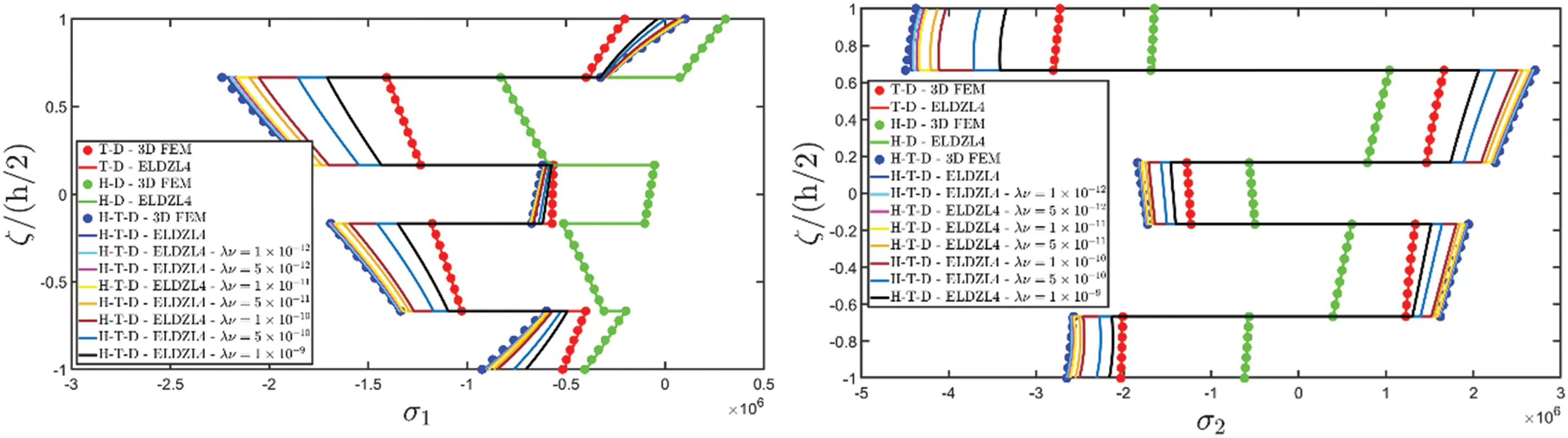

Figure 7: Through-the-thickness plots of the three-dimensional stress components of a simply-supported rectangular plate subjected to hygro-thermal sinusoidal loading with N~=M~=1. Effect of the coupling between the governing equations. Comparison to 3D FEM simulations. The results are provided for the point located at (s1,s2)=(0.25L1,0.25L2) within the physical domain
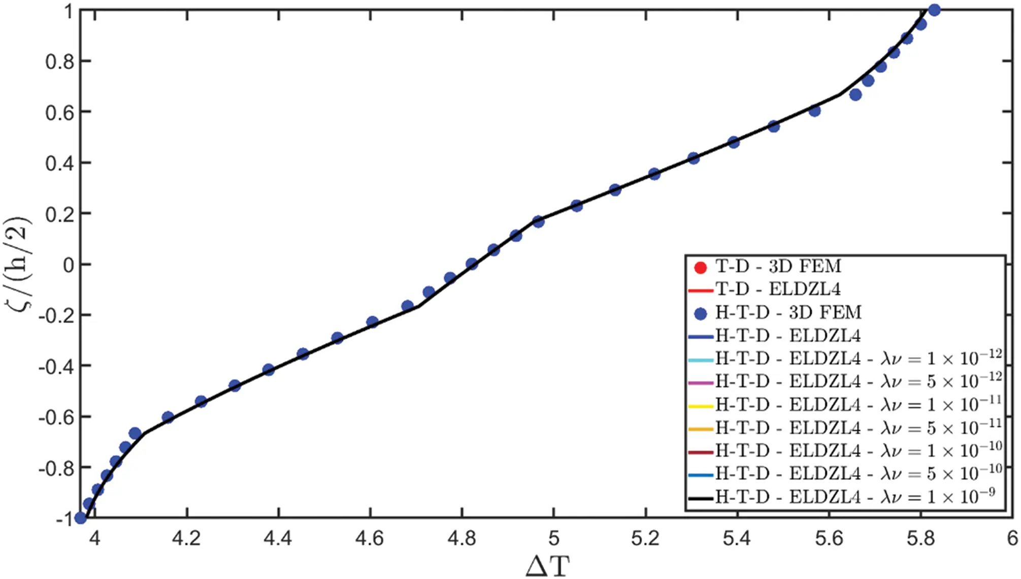

Figure 8: Through-the-thickness plots of the temperature variation and moisture concentration variation of a simply-supported rectangular plate subjected to hygro-thermal sinusoidal loading with N~=M~=1. Effect of the coupling between the governing equations. Comparison to 3D FEM simulations. The results are provided for the point located at (s1,s2)=(0.25L1,0.25L2) within the physical domain
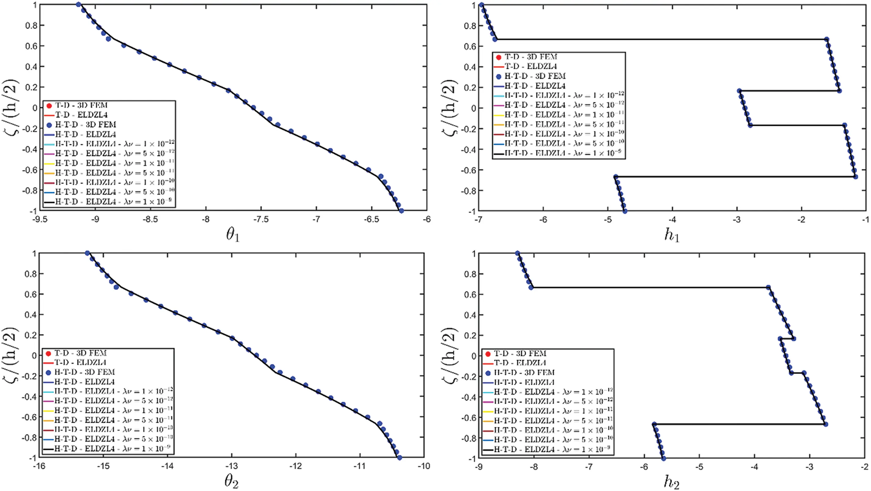

Figure 9: Through-the-thickness plots of the temperature gradient components (a) and thermal flux components (b) of a simply-supported rectangular plate subjected to hygro-thermal sinusoidal loading with N~=M~=1. Effect of the coupling between the governing equations. Comparison to 3D FEM simulations. The results are provided for the point located at (s1,s2)=(0.25L1,0.25L2) within the physical domain
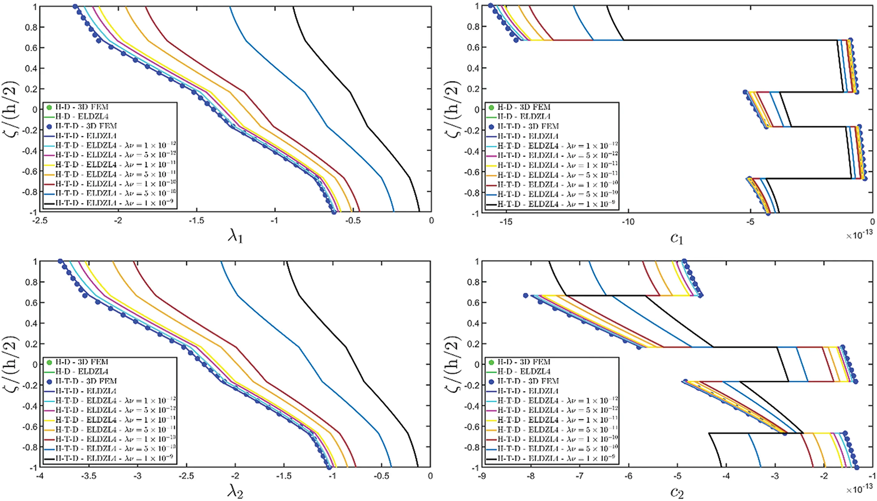

Figure 10: Through-the-thickness plots of the moisture diffusion gradient components (a) and hygrometric flux components (b) of a simply supported rectangular plate subjected to hygro-thermal sinusoidal loading with N~=M~=1. Effect of the coupling between the governing equations. Comparison to 3D FEM simulations. The results are provided for the point located at (s1,s2)=(0.25L1,0.25L2) within the physical domain
Two preliminary investigations account for the thermo-mechanical (T-D) and the hygro-mechanical (H-D) problems. The semi-analytical solution is derived using the ELDZL7 theory in which a higher-order polynomial is assumed along the thickness direction with N=7 and the ELW zigzag function (7). The results are compared with those coming from a 3D FEM model that employs 20-node brick elements characterized by 1820139 DOFs. External loads consist of a sinusoidal distribution of external thermal and hygrometric fluxes applied at the top and bottom surfaces characterized by N~=M~=1:
q¯Ts(+)=−10 J/m2,q¯Ts(−)=−6 J/m2q¯Cs(+)=−1.3063×10−12 kg/m2,q¯Cs(−)=−8.9194×10−13 kg/m2(113)
In addition to T-D and H-D simulations, an uncoupled hygro-thermo-mechanical (H-T-D) simulation is conducted with both the ELW two-dimensional model and the 3D FEM model. In other words, in this case, the additional deformations coming from the presence of hygro-thermal loads are considered, while coupling between thermal conduction and mass diffusion problem is denied. The Soret and Dufour coupling effects are, thus, neglected. In addition to T-D, H-D, and H-T-D simulations, some numerical investigations are performed with fully-coupled equations, including Dufour and Soret hygro-thermal effects. More specifically, a parametric investigation is performed in which different product values between the quantities ν are considered, ranging from 1×10⁻¹² to 1×10⁻⁹. As extensively shown in the work by Sih [25], the value of λν must be calibrated for experimental results. The value obtained here depends significantly on the hygro-thermal loading conditions and the material selected for the analysis. Hence, no general values can be provided which can be adopted in all laminated structures. Fig. 5 represents the through-the-thickness distribution of the displacement field components for the selected plate. As can be seen, the introduction of coupling between heat conduction and mass diffusion equations provides a significant variation in the deflection of the structure. If the uncoupled H-T-D deflection is essentially due to the sum of the thermal and hygrometric contributions, when Dufour and Soret phenomena are predicted by the model, a reduction in the magnitude of the upward bending response is noticed in both in-plane and out-of-plane components. Similar considerations are made for Fig. 6, which plots the strain components through the thickness direction. The hygro-thermal full coupling leads to minor deformations. The contribution from hygrometric loading is balanced because the structural response gradually varies from H-T-D results to T-D simulations in all deformation components. Fig. 7 shows the thickness plots for the three-dimensional stress components. It indicates that thermal and hygrometric loads induce additional stresses whose magnitudes are comparable to those obtained for an external mechanical pressure applied to the structure. Finally, Fig. 8 illustrates the through-the-thickness distribution of temperature and moisture concentration for the reference state of the structure. The presence of soft regions within the lamination scheme is also visible in this case because the profile of these configuration variables deviates from a conventional linear distribution, and a zigzag behavior is observed. This fact is found also in simulations with fully-coupled equations. In particular, in this case, a variation of the moisture concentration dispersion is noticed for an increased product value λν, while the temperature profile remains unvaried. This is because the Soret constants are higher than those associated with the Dufour phenomenon because, from a physical point of view, a positive temperature variation enables the migration of moisture within the solid. Therefore, water tends to leave the structure with a reduction in mass concentration. In contrast, an additional amount of moisture within the solid does not induce any significant variation in the overall temperature of the structure. This aspect can also be observed in plots of Fig. 9, representing the distribution of the temperature gradient and heat flux components. Based on these plots, the temperature gradient is the same for both T-D and H-T-D simulations. Even though the thermal generalized load is applied along the thickness direction, the orthotropic nature of the materials induces non-negligible in-plane thermal fluxes. In addition, the recovery procedure allows for the perfect fulfillment of the external loading conditions at the top and bottom surfaces of the panel. Finally, Fig. 10 collects the primary and secondary variables of the hygrometric equations. Unlike the corresponding quantities of the previous figure, the coupling between mass diffusion and thermal conduction equations is more clearly evident since different dispersions of mass concentration gradients and hygrometric fluxes are obtained, compared to uncoupled simulations. The lamination scheme with softcore induces the in-plane components derived from the uncoupled simulation to be very similar to those obtained with fully-coupled equations in the soft layers, while a more significant variation of the moisture flux is noticed in the remaining laminae.
A further investigation is then conducted on the plate, showing the influence of hygro-thermal loads on the overall deflection of the plate. More specifically, the panel is subjected to external loads with sinusoidal distribution, considering increasing magnitudes q¯Ts(+)=−10ψJ/m2,q¯Cs(+)=−1.3063×10−12ψkg/m2 and q¯Ts(−)=−6ψJ/m2,q¯Cs(−)=−8.9194×10−13ψkg/m2 at the top and bottom surfaces, respectively, being ψ a scale parameter. For each simulation, the overall deflection has been evaluated regarding the maximum value of the U3 displacement field component within the reference surface, located at ζ=0, for different magnitudes of the external loads. The results have been collected in Table 1. More specifically, the first column refers to pure hygro-mechanical simulations, while the first row contains the results from thermo-mechanical analysis. All the remaining cells contain the plate’s vertical deflection for various combinations of hygro-thermal loads. The results point out the linearity of the model. The fundamental Eq. (57) are developed so that an increase in the source variable results in an increase in the value of the configuration variables. Indeed, if the magnitude of both thermal and moisture diffusion loads doubles, even the displacement field components double. Similar considerations can be made also for strain and stress components.

At this point, the model is validated and adopted in the case of panels with single curvature. A cylindrical shell is, thus, considered, whose reference surface equation is reported in principal coordinates in Fig. 3. The lamination scheme is the same as in the rectangular plate of the previous simulation. In contrast, a Winkler foundation is modeled at the bottom surface, with an equal elastic spring stiffness k3f(−)=1×10⁸ Pa/m. Two different hydrostatic loads are applied to the structure. At the bottom surface, we apply a thermal and moisture flux of magnitude q¯Th(−)=−3 J/m2 and q¯Ch(−)=−8.9194×10⁻¹³ kg/m2, respectively, with a hydrostatic distribution along α1 the principal direction. Thermal and moisture fluxes of magnitude q¯Th(−)=−10 J/m2 and q¯Ch(+)=−2.3063×10⁻¹² kg/m2 are applied at the top surface with a hydrostatic variation along α2. Various simulations are performed on this structure with the present model for N~=M~=150, including T-D, H-D, and H-T-D simulations. The thickness plots, evaluated at the point in the physical domain located at (s1,s2)=(0.25L1,0.25L2), can be found in Figs. 11–16.

Figure 11: Through-the-thickness plots of the three-dimensional displacement field components of a circular cylinder lying on a Winkler foundation subjected to hygro-thermal hydrostatic loads along α1 and α2, evaluated for N~=M~=150. Effect of the coupling between the governing equations by means of Dufour and Soret effects. Comparison to 3D FEM simulations. The results are provided for the point located at (s1,s2)=(0.25L1,0.25L2) within the physical domain

Figure 12: Through-the-thickness plots of the three-dimensional strain components of a circular cylinder lying on a Winkler foundation subjected to hygro-thermal hydrostatic loads along α1 and α2, evaluated for N~=M~=150. Effect of the coupling between the governing equations using Dufour and Soret effects. Comparison with 3D FEM simulations. The results are provided for the point located at (s1,s2)=(0.25L1,0.25L2) within the physical domain

Figure 13: Through-the-thickness plots of the three-dimensional stress components of a circular cylinder lying on a Winkler foundation subjected to hygro-thermal hydrostatic loads along α1 and α2, evaluated for N~=M~=150. Effect of the coupling between the governing equations using Dufour and Soret effects. Comparison with 3D FEM simulations. The results are provided for the point located at (s1,s2)=(0.25L1,0.25L2) within the physical domain

Figure 14: Through-the-thickness plots of the temperature variation and moisture concentration variation for the reference state of a circular cylinder lying on a Winkler foundation subjected to hygro-thermal hydrostatic loads along α1 and α2, evaluated for N~=M~=150. Effect of the coupling between the governing equations using Dufour and Soret effects. Comparison with 3D FEM simulations. The results are provided for the point located at (s1,s2)=(0.25L1,0.25L2) within the physical domain

Figure 15: Through-the-thickness plots of the three-dimensional temperature gradient components (a) and thermal flux components (b) of a circular cylinder on a Winkler foundation subjected to hygro-thermal hydrostatic loads along α1 and α2, evaluated for N~=M~=150. Effect of the coupling between the governing equations using Dufour and Soret effects. Comparison with 3D FEM simulations. The results are provided for the point located at (s1,s2)=(0.25L1,0.25L2) within the physical domain

Figure 16: Through-the-thickness plots of the three-dimensional moisture concentration gradient components (a) and hygrometric flux components (b) of a circular cylinder lying on a Winkler foundation subjected to hygro-thermal hydrostatic loads along α1 and α2, evaluated for N~=M~=150. Effect of the coupling between the governing equations using Dufour and Soret effects. Comparison with 3D FEM simulations. The results are provided for the point located at (s1,s2)=(0.25L1,0.25L2) within the physical domain
As in the previous example, T-D, H-D, and uncoupled H-T-D numerical results are compared to those of a 3D FEM simulation of 765772 DOFs. A perfect agreement between the displacement field components obtained with the present formulation and those of the 3D FEM model is seen in Fig. 11. In addition, from a mechanical point of view, the presence of the Dufour and Soret coupling effect reduces the panel deflection, especially along the thickness direction and along α1, in the absence of curvatures. A variation of the strain components distribution due to a hygrothermal coupling is noticed in the strain components of Fig. 12. This behavior is particularly evident in the strain components, ε1,ε2, and ε3, while the variation of the shear strains γ13 and γ23 is noticed in the second and fourth layer, since the semi-analytical solution is found for the case of cross-ply stacking sequences and not for a general lamination scheme. In contrast, an excellent agreement is found with the reference solution. As far as the three-dimensional stress components are concerned, in Fig. 13, the hygrothermal stresses are very significant for the selected loading conditions, and the influence of the Dufour and Soret coupling is particularly evident in the case of in-plane stress components. At the same time, a similar profile is observed for the out-of-plane stresses. In addition, an increased out-of-plane normal stress coming from the elastic foundation is found at the bottom surface. Even in this simulation, a zigzag profile of temperature and moisture variation is derived, as shown in Fig. 14. An increase in temperature is found from the bottom to the top of the cylinder because it is assumed that a thermal flux heats the panel from its top lamina, while the loading condition at the bottom surface cools down the structure. This behavior is not varied by the presence of moisture concentration. On the other hand, the moisture distribution within the solid is influenced by the temperature distribution since the zigzag profile is gradually transformed into a straight vertical line. The variation of moisture profile due to an abrupt change of diffusion properties from a layer to its adjacent can be overcome by heating the structure.
Fig. 15 depicts the three-dimensional temperature gradient and thermal flux components for this example. It indicates that the semi-analytical solution with N~=M~=150 predicts well the outcomes of 3D FEM. In addition, more stable results are provided in the interlaminar region. The little discrepancy found for primary variables is not present in the case of secondary variables, where a perfect alignment exists among different approaches. Also, in this case, the results are not influenced by the Dufour and Soret coupling effect. In the case of moisture concentration gradients and hygrometric fluxes of Fig. 16, the results of hygro-thermo-elastic fully coupled simulations deviate from those of uncoupled models, especially for in-plane components. Finally, the loading conditions at the top and bottom surfaces are perfectly matched due to the adoption of the post-processing recovery procedure that employs the T-GDQ numerical method with IN=IM=31.
The last example investigates the hygro-thermo-elastic behavior of a laminated spherical panel. The geometric and material properties are detailed in Fig. 3. A mechanical loading is applied, whose magnitude q¯3u(+)=−7×10⁵ N/m2 is uniformly distributed along the top surface. The hygro-thermal loading conditions account for a patch distribution of thermal flux at the top surface with q¯Th(+)=−30 J/m2 characterized by (c10,d20)=(0.25L1,0.25L2) and (s10,s20)=(0.5L1,0.5L2), while hygrometric loads of magnitudes q¯Ch(+)=−2×10⁻¹² kg/m2 and q¯Ch(−)=−6×10⁻¹² kg/m2 are characterized by a hydrostatic distribution along α1 and α2, respectively. Finally, the value ΔT(−)=0K is prescribed at the bottom surface by means of the ELW thickness functions of Eq. (6). In addition, an elastic foundation is present at the bottom surface, modeled with the Winkler-Pasternak model of Eq. (48), where the elastic spring stiffnesses are k1f(−)=k2f(−)=5×10⁷ Pa/m and k3f(−)=5×10⁸ Pa/m, while the shear modulus is set equal to Gf(−)=5×10⁶Pa. Thickness plots, collected in Figs. 17–22, are evaluated with the ELDZL7 kinematic model with the present formulation setting N~=M~=150. Fig. 17 depicts the thickness plots for the displacement field components. As can be seen here, introducing a generally distributed hygrothermal external load exhibits a variation of deflection of the shell, while the stretching behavior remains almost unvaried. Note that the zigzag effect, though present, is less evident as in the previous examples. In addition, a change of U2 slope is found when the value of the product λν increases, while the variation in U1 profile is less evident. Three-dimensional strain components are reported in Fig. 18, showing that the axial strain along α2 varies for the mechanical case under a hygrothermal load. Adding hygrothermal coupling terms within the fundamental equations induces a variation in the slope of γ12, which becomes more evident as the quantity λν increases. In the same way, various γ23 thickness plots are found in all these simulations, even though the kinematic equations are always respected at the top and bottom surfaces once the post-processing multifield procedure is applied. In Fig. 19, the three-dimensional stress components of the spherical shell are collected. More specifically, it is shown that σ1 exhibits an unusual slope change of its profile in the central core of the structure, while σ2 distribution is not characterized by this peculiarity. On the other hand, shear stress distributions obtained from the mechanical elasticity simulation are varied when hygro-thermal loads are applied to the structure. Instead, σ3 component is not significantly influenced by these external actions. As far as the effect of the Winkler-Pasternak elastic foundation is concerned, the influence of linear springs is more clearly evident than that of the shear layer.

Figure 17: Through-the-thickness plots of the three-dimensional displacement field components of a spherical panel lying on a Winkler-Pasternak foundation subjected to uniformly-distributed mechanical loads, hydrostatic hygrometric loads, a prescribed value of temperature and patch-distributed thermal flux evaluated for N~=M~=150. Effect of the coupling between the governing equations using Dufour and Soret effects. Comparison with 3D FEM simulations. The results are provided for the point located at (s1,s2)=(0.25L1,0.25L2) within the physical domain

Figure 18: Through-the-thickness plots of the three-dimensional strain components of a spherical panel lying on a Winkler-Pasternak foundation subjected to uniformly-distributed mechanical loads, hydrostatic hygrometric loads, a prescribed value of temperature and patch-distributed thermal flux evaluated for N~=M~=150. Effect of the coupling between the governing equations utilizing Dufour and Soret effects. Comparison with 3D FEM simulations. The results are provided for the point located at (s1,s2)=(0.25L1,0.25L2) within the physical domain

Figure 19: Through-the-thickness plots of the three-dimensional stress components of a spherical panel lying on a Winkler-Pasternak foundation subjected to uniformly-distributed mechanical loads, hydrostatic hygrometric loads, a prescribed value of temperature and patch-distributed thermal flux evaluated for N~=M~=150. Effect of the coupling between the governing equations utilizing Dufour and Soret effects. Comparison with 3D FEM simulations. The results are provided for the point located at (s1,s2)=(0.25L1,0.25L2) within the physical domain

Figure 20: Through-the-thickness plots of the temperature variation and of a moisture variation with respect to the reference state of a spherical panel lying on a Winkler-Pasternak foundation subjected to uniformly distributed mechanical loads, hydrostatic hygrometric loads, a prescribed value of temperature and patch-distributed thermal flux evaluated for N~=M~=150. Effect of the coupling between the governing equations by means of Dufour and Soret effects. Comparison with 3D FEM simulations. The results are provided for the point located at (s1,s2)=(0.25L1,0.25L2) within the physical domain

Figure 21: Through-the-thickness plots of the temperature gradient components (a) and of the thermal flux components (b) of a spherical panel lying on a Winkler-Pasternak foundation subjected to uniformly distributed mechanical loads, hydrostatic hygrometric loads, a prescribed value of temperature and patch-distributed thermal flux evaluated for N~=M~=150. Effect of the coupling between the governing equations utilizing Dufour and Soret effects. Comparison with 3D FEM simulations. The results are provided for the point located at (s1,s2)=(0.25L1,0.25L2) within the physical domain

Figure 22: Through-the-thickness plots of the moisture concentration gradient components (a) and of the hygrometric flux components (b) of a spherical panel lying on a Winkler-Pasternak foundation subjected to uniformly-distributed mechanical loads, hydrostatic hygrometric loads, a prescribed value of temperature and patch-distributed thermal flux evaluated for N~=M~=150. Effect of the coupling between the governing equations utilizing Dufour and Soret effects. Comparison with 3D FEM simulations. The results are provided for the point located at (s1,s2)=(0.25L1,0.25L2) within the physical domain
Unlike the displacement field components of Fig. 17, the temperature and moisture concentration variation thickness plots shown in Fig. 20 exhibit a typical zigzag behavior in all simulations. The prescribed temperature at the bottom surface is always respected. On the other hand, Dufour and Soret coupling enables scaling of the mass concentration dispersion along the thickness direction. In particular, the hygrometric configuration variable exhibits a vertical distribution for increased coupling of the equations by quantities. Hygro-thermal primary and secondary variables can be found in Figs. 21 and 22. In particular, the same temperature gradient components and thermal fluxes distributions exhibit a significantly nonlinear aspect, along with zigzag effects. In addition, the same results are obtained in both uncoupled and coupled hygro-thermal numerical investigations. For the moisture flux components in Fig. 22, the c3 distribution always fulfills the loading conditions at the top and bottom surfaces, and only a slight deviation from the uncoupled structural behavior is found for coupled simulations. In contrast, the λ3 thickness plot depends significantly on the choice of product λν. As far as λ1 and λ2 are concerned, introducing Dufour-Soret effects leads to a significant variation of results. In addition, a zigzag response is induced in some interlaminar regions, while in other ones, this structural behavior is balanced, with a smoother distribution.
8 Conclusions
The study investigates the hygro-thermo-mechanical response of doubly-curved solids using a refined two-dimensional formulation with curvilinear principal coordinates, where an innovative ELW kinematic model is introduced in which arbitrary values of the configuration variables are prescribed at the top and bottom surfaces of the solid. In addition, a generalized distribution of external loads is applied, accounting for surface tractions, thermal fluxes, and mass fluxes. Unlike most recent research on the topic, the fundamental equations in this study account for the full coupling between the displacement field, temperature, and moisture concentration through hygrothermal expansion constants, along with Dufour and Soret effects. A semi-analytical solution is provided using Navier’s method, and an efficient recovery procedure based on the hygro-thermo-mechanical balance equations is adopted to derive the three-dimensional response of the laminated panel from a two-dimensional solution. Therefore, the solution is suitable for simply supported panels with uniform curvature and cross-ply lamination scheme, whereas a possible enhancement of the model can be its numerical implementation involving further boundary conditions, variable curvature, and lamination scheme. The formulation is validated and applied in some examples involving structures of different geometric shapes. Uncoupled simulations are successfully compared to those of a 3D FEM model developed with commercial software. Then, useful parametric investigations are performed to show the influence of hygro-thermal coupling. This parametric analysis aims to demonstrate that hygro-thermal coupling can affect the mechanical response of laminated structures as the model can predict this additional response. The results, provided for different values of coupling coefficients, should be calibrated against experimental results to evaluate the effective deviation from those associated with uncoupled simulations for practical applications. The present formulation is a valid tool for predicting the response of doubly-curved panels simultaneously subjected to mechanical and hygro-thermal loading conditions.
Acknowledgement: The authors are grateful to the Department of Innovation Engineering for their constant support.
Funding Statement: The paper has been funded by the Project PNRR M4C2—Innovation grant DIRECT: Digital twIns foR EmergenCy supporT—CUP F83C22000740001.
Author Contributions: Francesco Tornabene: Writing—review & editing, Visualization, Validation, Supervision, Software, Methodology, Investigation, Formal analysis, Data curation, Conceptualization. Matteo Viscoti: Writing—original draft, Validation, Investigation, Data curation. Rossana Dimitri: Writing—review & editing, Validation, Supervision, Investigation, Formal analysis, Conceptualization. All authors reviewed the results and approved the final version of the manuscript.
Availability of Data and Materials: All data generated or analyzed during this study are included in this published article.
Ethics Approval: Not applicable.
Conflicts of Interest: The authors declare no conflicts of interest to report regarding the present study.
References
1. Fernandes O, Dutta J, Pai Y. Effect of various factors and hygrothermal ageing environment on the low velocity impact response of fibre reinforced polymer composites-a comprehensive review. Cogent Eng. 2023;10(1):2247228. doi:10.1080/23311916.2023.2247228. [Google Scholar] [CrossRef]
2. Aceti P, Carminati L, Bettini P, Sala G. Hygrothermal ageing of composite structures. Part 1: technical review. Compos Struct. 2023;319(1):117076. doi:10.1016/j.compstruct.2023.117076. [Google Scholar] [CrossRef]
3. Patel BP, Ganapathi M, Makhecha DP. Hygrothermal effects on the structural behaviour of thick composite laminates using higher-order theory. Compos Struct. 2002;56(1):25–34. doi:10.1016/S0263-8223(01)00182-9. [Google Scholar] [CrossRef]
4. Lo SH, Zhen W, Cheung YK, Chen WJ. Hygrothermal effects on multilayered composite plates using a refined higher order theory. Compos Struct. 2010;92(3):633–46. doi:10.1016/j.compstruct.2009.09.034. [Google Scholar] [CrossRef]
5. Jones RM. Mechanics of composite materials. Philadelphia: CRC Press; 1999. [Google Scholar]
6. Barbero EJ. Introduction to composite materials design. Boca Raton: CRC Press; 2010. [Google Scholar]
7. Gay D. Composite materials: design and applications. Boca Raton: CRC Press; 2022. [Google Scholar]
8. Biswal M, Sahu SK, Asha AV. Experimental and numerical studies on free vibration of laminated composite shallow shells in hygrothermal environment. Compos Struct. 2015;127(1):165–74. doi:10.1016/j.compstruct.2015.03.007. [Google Scholar] [CrossRef]
9. Richeton J, Schlatter G, Vecchio KS, Rémond Y, Ahzi S. A unified model for stiffness modulus of amorphous polymers across transition temperatures and strain rates. Polymer. 2005;46(19):8194–201. doi:10.1016/j.polymer.2005.06.103. [Google Scholar] [CrossRef]
10. Gholami M, Afrasiab H, Baghestani AM, Fathi A. Hygrothermal degradation of elastic properties of fiber reinforced composites: a micro-scale finite element analysis. Compos Struct. 2021;266(1):113819. doi:10.1016/j.compstruct.2021.113819. [Google Scholar] [CrossRef]
11. Garg A, Chalak HD. A review on analysis of laminated composite and sandwich structures under hygrothermal conditions. Thin-Walled Struct. 2019;142(1):205–26. doi:10.1016/j.tws.2019.05.005. [Google Scholar] [CrossRef]
12. Tornabene F. Hygro-thermo-magneto-electro-elastic theory of anisotropic doubly-curved shells. Esculapio: Bologna; 2023. [Google Scholar]
13. Zheng YF, Kang CC, Xu LL, Chen CP. Nonlinear analysis of rectangular magnetoelectroelastic moderately thick laminated plates under multifield coupling loads. Thin-Walled Struct. 2022;177(1):109406. doi:10.1016/j.tws.2022.109406. [Google Scholar] [CrossRef]
14. Barakati A, Zhupanska OI. Mechanical response of electrically conductive laminated composite plates in the presence of an electromagnetic field. Compos Struct. 2014;113(1):298–307. doi:10.1016/j.compstruct.2014.03.020. [Google Scholar] [CrossRef]
15. Brischetto S, Cesare D. Hygro-elastic coupling in a 3D exact shell model for bending analysis of layered composite structures. J Compos Sci. 2023;7(5):183. doi:10.3390/jcs7050183. [Google Scholar] [CrossRef]
16. Brischetto S, Torre R. 3D hygro-elastic shell model for the analysis of composite and sandwich structures. Compos Struct. 2022;285(1):115162. doi:10.1016/j.compstruct.2021.115162. [Google Scholar] [CrossRef]
17. Júnior MT, Zilio G, Mortean MVV, De Paiva KV, Oliveira JLG. Experimental and numerical analysis of transient thermal stresses on thick-walled cylinder. Int J Press Vessel Pip. 2023;202(1):104884. doi:10.1016/j.ijpvp.2023.104884. [Google Scholar] [CrossRef]
18. Elfar M, Sedaghati R, Abdelsalam OR. Transient coupled thermo-elasticity analysis of a temperature-dependent thick-walled cylinder under cyclic thermo-mechanical loads. SN Appl Sci. 2023;5(1):9. doi:10.1007/s42452-022-05228-0. [Google Scholar] [CrossRef]
19. Szekeres A. Analogy between heat and moisture: thermo-hygro-mechanical tailoring of composites by taking into account the second sound phenomenon. Comput Struct. 2000;76(1–3):145–52. doi:10.1016/S0045-7949(99)00170-4. [Google Scholar] [CrossRef]
20. Szekeres A, Engelbrecht J. Coupled thermal and moisture fields with application to composites. Period Polytech Mech Eng. 1997;41(2):151–61. [Google Scholar]
21. Brischetto S. Hygrothermal loading effects in bending analysis of multilayered composite plates. Comput Model Eng Sci. 2012;88(5):367–417. doi:10.3970/CMES.2012.088.367. [Google Scholar] [CrossRef]
22. Tounsi A, Bedia EA, Benachour A. A new computational method for prediction of transient hygroscopic stresses during moisture desorption in laminated composite plates with different degrees of anisotropy. J Thermoplast Compos Mater. 2005;18(1):37–58. doi:10.1177/0892705705041156. [Google Scholar] [CrossRef]
23. Xie H, Gong G, Wu Y. Investigations of equilibrium moisture content with Kelvin modification and dimensional analysis method for composite hygroscopic material. Constr Build Mater. 2017;139(1):101–13. doi:10.1016/j.conbuildmat.2017.02.018. [Google Scholar] [CrossRef]
24. Choi HS, Ahn KJ, Nam JD, Chun HJ. Hygroscopic aspects of epoxy/carbon fiber composite laminates in aircraft environments. Compos-A: Appl Sci Manuf. 2001;32(5):709–20. doi:10.1016/S1359-835X(00)00145-7. [Google Scholar] [CrossRef]
25. Sih GC, Michopoulos J, Chou SC. Hygrothermoelasticity. Dordrecht: Springer Science & Business Media; 2012. [Google Scholar]
26. Sih GC, Shih MT, Chou SC. Transient hygrothermal stresses in composites: coupling of moisture and heat with temperature varying diffusivity. Int J Eng Sci. 1980;18(1):19–42. doi:10.1016/0020-7225(80)90004-X. [Google Scholar] [CrossRef]
27. Sih GC, Ogawa A. Transient thermal change on a solid surface: coupled diffusion of heat and moisture. J Therm Stresses. 1982;5(3–4):265–82. doi:10.1080/01495738208942150. [Google Scholar] [CrossRef]
28. Onsager L. Reciprocal relations in irreversible processes I–II. Phys Rev. 1931;37(4):405–426. doi:10.1103/PhysRev.37.405. [Google Scholar] [CrossRef]
29. Platten JK. The Soret effect: a review of recent experimental results. J Appl Mech. 2006;73(1):5–15. doi:10.1115/1.1992517. [Google Scholar] [CrossRef]
30. Eastman ED. Theory of the Soret effect. J Am Chem Soc. 1928;50(2):283–91. doi:10.1021/ja01389a007. [Google Scholar] [CrossRef]
31. Ingle SE, Horne FH. The Dufour effect. J Chem Phys. 1973;59(11):5882–94. doi:10.1063/1.1679957. [Google Scholar] [CrossRef]
32. Meenakshi V. Dufour and soret effect on unsteady MHD free convection and mass transfer flow past an impulsively started vertical porous plate considering with heat generation. J Heat Mass Transf Res. 2021;8(2):257–66. doi:10.22075/jhmtr.2021.21229.1301. [Google Scholar] [CrossRef]
33. Vaddadi P, Nakamura T, Singh RP. Transient hygrothermal stresses in fiber reinforced composites: a heterogeneous characterization approach. Compos-A: Appl Sci Manuf. 2003;34(8):719–30. doi:10.1016/S1359-835X(03)00135-0. [Google Scholar] [CrossRef]
34. Pipes RB, Vinson JR, Chou TW. On the hygrothermal response of laminated composite systems. J Compos Mater. 1976;10(2):129–48. doi:10.1177/002199837601000203. [Google Scholar] [CrossRef]
35. Yüksel YZ, Akbaş D. Hygrothermal stress analysis of laminated composite porous plates. Struct Eng Mech. 2021;80(1):1–13. doi:10.12989/sem.2021.80.1.001. [Google Scholar] [CrossRef]
36. Tornabene F, Viscoti M, Dimitri R. Equivalent layer-wise theory for the hygro-thermo-magneto-electro-elastic analysis of laminated curved shells. Thin-Walled Struct. 2024;198(1):111751. doi:10.1016/j.tws.2024.111751. [Google Scholar] [CrossRef]
37. Liu Z, Reinoso J, Paggi M. Hygro-thermo-mechanical modeling of thin-walled photovoltaic laminates with polymeric interfaces. J Mech Phys Solids. 2022;169(1):105056. doi:10.1016/j.jmps.2022.105056. [Google Scholar] [CrossRef]
38. Brischetto S. Hygrothermoelastic analysis of multilayered composite and sandwich shells. J Sandw Struct Mater. 2013;15(2):168–202. doi:10.1177/1099636212471358. [Google Scholar] [CrossRef]
39. Brischetto S, Cesare D. A coupled hygro-elastic 3D model for steady-state analysis of functionally graded plates and shells. Curved Layer Struct. 2023;10(1):20220216. doi:10.1515/cls-2022-0216. [Google Scholar] [CrossRef]
40. Ye T, Jin G, Gao S. Three-dimensional hygrothermal vibration of multilayered cylindrical shells. Compos Struct. 2018;201(1):867–81. doi:10.1016/j.compstruct.2018.06.055. [Google Scholar] [CrossRef]
41. Arefi M, Moghaddam SK, Bidgoli EMR, Kiani M, Civalek O. Analysis of graphene nanoplatelet reinforced cylindrical shell subjected to thermo-mechanical loads. Compos Struct. 2021;255(1):112924. doi:10.1016/j.compstruct.2020.112924. [Google Scholar] [CrossRef]
42. Nam VH, Dong DT, Phuong NT, Tuan HD. Nonlinear thermo-mechanical stability of multilayer-FG plates reinforced by orthogonal and oblique stiffeners according to FSDT. J Reinf Plast Compos. 2019;38(11):521–36. doi:10.1177/0731684419831650. [Google Scholar] [CrossRef]
43. Ebrahimi F, Shafiei N, Kazemi M, Mousavi Abdollahi SM. Thermo-mechanical vibration analysis of rotating nonlocal nanoplates applying generalized differential quadrature method. Mech Adv Mater Struct. 2017;24(15):1257–73. doi:10.1080/15376494.2016.1227499. [Google Scholar] [CrossRef]
44. Sai Charan M, Naik AK, Kota N, Laha T, Roy S. Review on developments of bulk functionally graded composite materials. Int Mater Rev. 2022;67(8):797–863. doi:10.1080/09506608.2022.2026863. [Google Scholar] [CrossRef]
45. Pélegris C, Ferguen N, Leclerc W, Lorgouilloux Y, Hocquet S, Rigo O, et al. Thermal conductivity modelling of alumina/Al functionally graded composites. Can J Chem Eng. 2015;93(2):192–200. doi:10.1002/cjce.22091. [Google Scholar] [CrossRef]
46. Eldeeb AM, Shabana YM, El-Sayed TA, Guo L, Elsawaf A. Thermoelastic stresses alleviation for two-dimensional functionally graded cylinders under asymmetric loading. J Therm Stresses. 2023;46(1):59–74. doi:10.1080/01495739.2022.2151960. [Google Scholar] [CrossRef]
47. Ghatage PS, Kar VR, Sudhagar PE. On the numerical modelling and analysis of multi-directional functionally graded composite structures: a review. Compos Struct. 2020;236(1):111837. doi:10.1016/j.compstruct.2019.111837. [Google Scholar] [CrossRef]
48. Tornabene F. Free vibration analysis of functionally graded conical, cylindrical shell and annular plate structures with a four-parameter power-law distribution. Comput Methods Appl Mech Eng. 2009;198(37–40):2911–35. doi:10.1016/j.cma.2009.04.011. [Google Scholar] [CrossRef]
49. Tornabene F, Viscoti M, Dimitri R. Higher order theories for the modal analysis of anisotropic doubly-curved shells with a three-dimensional variation of the material properties. Eng Anal Bound Elem. 2024;158(1):486–519. doi:10.1016/j.enganabound.2023.11.008. [Google Scholar] [CrossRef]
50. Tornabene F, Viscoti M, Dimitri R. Effect of porosity on the modal response of doubly-curved laminated shell structures made of functionally graded materials employing higher order theories. Structure. 2024;60(1):105848. doi:10.1016/j.istruc.2023.105848. [Google Scholar] [CrossRef]
51. Belabed Z, Houari MSA, Tounsi A, Mahmoud SR, Bég OA. An efficient and simple higher order shear and normal deformation theory for functionally graded material (FGM) plates. Compos B: Eng. 2014;60(1):274–83. doi:10.1016/j.compositesb.2013.12.057. [Google Scholar] [CrossRef]
52. Kumar R, Lal A, Singh BN, Singh J. Non-linear analysis of porous elastically supported FGM plate under various loading. Compos Struct. 2020;233(1):111721. doi:10.1016/j.compstruct.2019.111721. [Google Scholar] [CrossRef]
53. Subramanian P. Dynamic analysis of laminated composite beams using higher order theories and finite elements. Compos Struct. 2006;73(3):342–53. doi:10.1016/j.compstruct.2005.02.002. [Google Scholar] [CrossRef]
54. Bhaskar K, Varadan TK. Refinement of higher-order laminated plate theories. AIAA J. 1989;27(12):1830–1. doi:10.2514/3.10345. [Google Scholar] [CrossRef]
55. Cho M, Parmerter RR. An efficient higher-order plate theory for laminated composites. Compos Struct. 1992;20(2):113–23. doi:10.1016/0263-8223(92)90067-M. [Google Scholar] [CrossRef]
56. Kant T, Swaminathan K. Analytical solutions for the static analysis of laminated composite and sandwich plates based on a higher order refined theory. Compos Struct. 2002;56(4):329–44. doi:10.1016/S0263-8223(02)00017-X. [Google Scholar] [CrossRef]
57. Brischetto S, Torre R, Cesare D. Three-dimensional coupling between elastic and thermal fields in the static analysis of multilayered composite shells. Comput Model Eng Sci. 2023;136(3):2551–94. doi:10.32604/cmes.2023.026312. [Google Scholar] [CrossRef]
58. Brischetto S, Torre R. 3D shell model for the thermo-mechanical analysis of FGM structures via imposed and calculated temperature profiles. Aerosp Sci Technol. 2019;85(1):125–49. doi:10.1016/j.ast.2018.12.011. [Google Scholar] [CrossRef]
59. Papadopoulos AM. State of the art in thermal insulation materials and aims for future developments. Energy Build. 2005;37(1):77–86. doi:10.1016/j.enbuild.2004.05.006. [Google Scholar] [CrossRef]
60. Fricke J, Schwab H, Heinemann U. Vacuum insulation panels-exciting thermal properties and most challenging applications. Int J Thermophys. 2006;27(1):1123–39. doi:10.1007/s10765-006-0106-6. [Google Scholar] [CrossRef]
61. Murakami H. Laminated composite plate theory with improved in-plane responses. J Appl Mech. 1986;53(3):661–6. doi:10.1115/1.3171828. [Google Scholar] [CrossRef]
62. Toledano A, Murakami H. A high-order laminated plate theory with improved in-plane responses. Int J Solids Struct. 1987;23(1):111–31. doi:10.1016/0020-7683(87)90034-5. [Google Scholar] [CrossRef]
63. Reddy JN, Liu C. A higher-order shear deformation theory of laminated elastic shells. Int J Eng Sci. 1985;23(3):319–30. doi:10.1016/0020-7225(85)90051-5. [Google Scholar] [CrossRef]
64. Reddy JN, Wang C, Lee KH. Relationships between bending solutions of classical and shear deformation beam theories. Int J Solids Struct. 1997;34(26):3373–84. doi:10.1016/S0020-7683(96)00211-9. [Google Scholar] [CrossRef]
65. Reddy JN. Exact solutions of moderately thick laminated shells. J Eng Mech. 1984;110(5):794–809. doi:10.1061/(ASCE)0733-9399(1984)110:5(794). [Google Scholar] [CrossRef]
66. Reddy JN. A generalization of two-dimensional theories of laminated composite plates. Commun Pure Appl Math. 1987;3(3):173–80. doi:10.1016/0263-8223(92)90026-9. [Google Scholar] [CrossRef]
67. Reddy JN. On the generalization of displacement-based laminate theories. Appl Mech Rev. 1989;42(11S):S213–22. doi:10.1115/1.3152393. [Google Scholar] [CrossRef]
68. Reddy JN. An evaluation of equivalent-single-layer and layerwise theories of composite laminates. Compos Struct. 1993;25(1–4):21–35. doi:10.1016/0263-8223(93)90147-I. [Google Scholar] [CrossRef]
69. Abrate S, Di Sciuva M. Equivalent single layer theories for composite and sandwich structures: a review. Compos Struct. 2017;179(1):482–94. doi:10.1016/j.compstruct.2017.07.090. [Google Scholar] [CrossRef]
70. Tornabene F, Viscoti M, Dimitri R, Reddy JN. Higher order theories for the vibration study of doubly-curved anisotropic shells with a variable thickness and isogeometric mapped geometry. Compos Struct. 2021;267(1):113829. doi:10.1016/j.compstruct.2022.115740. [Google Scholar] [CrossRef]
71. Tornabene F, Viscoti M, Dimitri R. Static analysis of anisotropic doubly-curved shell subjected to concentrated loads employing higher order layer-wise theories. Comput Model Eng Sci. 2023;134(2):1393–468. doi:10.32604/cmes.2022.022237. [Google Scholar] [CrossRef]
72. Tornabene F, Viscoti M, Dimitri R. On the importance of the recovery procedure in the semi-analytical solution for the static analysis of curved laminated panels: comparison with 3D finite elements. Materials. 2024;17(3):588. doi:10.3390/ma17030588. [Google Scholar] [PubMed] [CrossRef]
73. Tornabene F, Fantuzzi N, Bacciocchi M, Reddy JN. An equivalent layer-wise approach for the free vibration analysis of thick and thin laminated and sandwich shells. Appl Sci. 2016;7(1):17. doi:10.3390/app7010017. [Google Scholar] [CrossRef]
74. Tornabene F, Viscoti M, Dimitri R. Free vibration analysis of laminated doubly-curved shells with arbitrary material orientation distribution employing higher order theories and differential quadrature method. Eng Anal Bound Elem. 2023;152(1):397–445. doi:10.1016/j.enganabound.2023.04.008. [Google Scholar] [CrossRef]
75. Tornabene F, Viscoti M, Dimitri R, Aiello MA. Higher-order modeling of anisogrid composite lattice structures with complex geometries. Eng Struct. 2021;244(1):112686. doi:10.1016/j.engstruct.2021.112686. [Google Scholar] [CrossRef]
76. Tornabene F, Viscoti M, Dimitri R, Aiello MA. Higher order formulations for doubly-curved shell structures with a honeycomb core. Thin-Walled Struct. 2021;164(1):107789. doi:10.1016/j.tws.2021.107789. [Google Scholar] [CrossRef]
77. Shu C, Richards BE. Application of generalized differential quadrature to solve two-dimensional incompressible Navier-Stokes equations. Int J Numer Methods Fluids. 1992;15(7):791–8. doi:10.1002/fld.1650150704. [Google Scholar] [CrossRef]
78. Tornabene F. Generalized differential and integral quadrature. Esculapio: Bologna; 2023. [Google Scholar]
79. Shu C, Du H. Free vibration analysis of laminated composite cylindrical shells by DQM. Compos B: Eng. 1997;28(3):267–74. doi:10.1016/S1359-8368(96)00052-2. [Google Scholar] [CrossRef]
80. Shu C, Du H. Implementation of clamped and simply supported boundary conditions in the GDQ free vibration analysis of beams and plates. Int J Solids Struct. 1997;34(7):819–35. doi:10.1016/S0020-7683(96)00057-1. [Google Scholar] [CrossRef]
81. Shu C, Chew YT. On the equivalence of generalized differential quadrature and highest order finite difference scheme. Comput Methods Appl Mech Eng. 1998;155(3–4):249–60. doi:10.1016/S0045-7825(97)00150-3. [Google Scholar] [CrossRef]
82. Shu C. Free vibration analysis of composite laminated conical shells by generalized differential quadrature. J Sound Vib. 1996;194(4):587–604. doi:10.1006/jsvi.1996.0379. [Google Scholar] [CrossRef]
83. Tornabene F, Fantuzzi N, Ubertini F, Viola E. Strong formulation finite element method based on differential quadrature: a survey. Appl Mech Rev. 2015;67(2):020801. doi:10.1115/1.4028859. [Google Scholar] [CrossRef]
84. Tornabene F, Viscoti M, Dimitri R. Equivalent single layer higher order theory based on a weak formulation for the dynamic analysis of anisotropic doubly-curved shells with arbitrary geometry and variable thickness. Thin-Walled Struct. 2022;174(1):109119. doi:10.1016/j.tws.2022.109119. [Google Scholar] [CrossRef]
85. Fazzolari FA, Viscoti M, Dimitri R, Tornabene F. 1D-Hierarchical Ritz and 2D-GDQ Formulations for the free vibration analysis of circular/elliptical cylindrical shells and beam structure. Compos Struct. 2021;258(1):113338. doi:10.1016/j.compstruct.2020.113338. [Google Scholar] [CrossRef]
86. Reddy JN. Mechanics of laminated composite plates and shells: theory and analysis. Boca Raton: CRC Press; 2003. [Google Scholar]
87. Li H, Pang F, Wang X, Du Y, Chen H. Free vibration analysis for composite laminated doubly-curved shells of revolution by a semi analytical method. Compos Struct. 2018;201(1):86–111. doi:10.1016/j.compstruct.2018.05.143. [Google Scholar] [CrossRef]
Appendix A
This section presents the extended expression, reported in matrix form in Eq. (44), of the generalized higher-order secondary variables of the formulation, which are the elements of the vector Σ(τ)αi. These quantities are expressed in terms of the hygro-thermo-mechanical configuration variables of the model, which are arranged in vector δ(η), with η=0,…,N+1.
N1(τ)αi=∑η=0N+1((A11(20)(τη)[00]αiα1A1∂∂α1+A12(11)(τη)[00]αiα1A1A2∂A2∂α1−A16(20)(τη)[00]αiα1A1A2∂A1∂α2+A16(11)(τη)[00]αiα1A2∂∂α2−A14(20)(τη)[00]αiα1R1+A14(10)(τη)[01]αiα1)u1(η)++(A11(20)(τη)[00]αiα2A1A2∂A1∂α2+A12(11)(τη)[00]αiα2A2∂∂α2+A16(20)(τη)[00]αiα2A1∂∂α1−A16(11)(τη)[00]αiα2A1A2∂A2∂α1−A15(11)(τη)[00]αiα2R2+A15(10)(τη)[01]αiα2)u2(η)++(A11(20)(τη)[00]αiα3R1+A12(11)(τη)[00]αiα3R2+A14(20)(τη)[00]αiα3A1∂∂α1+A15(11)(τη)[00]αiα3A2∂∂α2+A13(10)(τη)[01]αiα3)u3(η)−Z11(10)(τη)[00]αiα4ξ(η)−E11(10)(τη)[00]αiα5κ(τ))
N2(τ)αi=∑η=0N+1((A12(11)(τη)[00]αiα1A1∂∂α1+A22(02)(τη)[00]αiα1A1A2∂A2∂α1−A26(11)(τη)[00]αiα1A1A2∂A1∂α2+A26(02)(τη)[00]αiα1A2∂∂α2−A24(11)(τη)[00]αiα1R1+A24(01)(τη)[01]αiα1)u1(η)++(A12(11)(τη)[00]αiα2A1A2∂A1∂α2+A22(02)(τη)[00]αiα2A2∂∂α2+A26(11)(τη)[00]αiα2A1∂∂α1−A26(02)(τη)[00]αiα2A1A2∂A2∂α1−A25(02)(τη)[00]αiα2R2+A25(01)(τη)[01]αiα2)u2(η)++(A12(11)(τη)[00]αiα3R1+A22(02)(τη)[00]αiα3R2+A24(11)(τη)[00]αiα3A1∂∂α1+A25(02)(τη)[00]αiα3A2∂∂α2+A23(01)(τη)[01]αiα3)u3(η)−Z22(01)(τη)[00]αiα4ξ(η)−E22(01)(τη)[00]αiα5κ(η))
N12(τ)αi=∑η=0N+1((A16(20)(τη)[00]αiα1A1∂∂α1+A26(11)(τη)[00]αiα1A1A2∂A2∂α1−A66(20)(τη)[00]αiα1A1A2∂A1∂α2+A66(11)(τη)[00]αiα1A2∂∂α2−A46(20)(τη)[00]αiα1R1+A46(10)(τη)[01]αiα1)u1(η)++(A16(20)(τη)[00]αiα2A1A2∂A1∂α2+A26(11)(τη)[00]αiα2A2∂∂α2+A66(20)(τη)[00]αiα2A1∂∂α1−A66(11)(τη)[00]αiα2A1A2∂A2∂α1−A56(11)(τη)[00]αiα2R2+A56(10)(τη)[01]αiα2)u2(η)++(A16(20)(τη)[00]αiα3R1+A26(11)(τη)[00]αiα3R2+A46(20)(τη)[00]αiα3A1∂∂α1+A56(11)(τη)[00]αiα3A2∂∂α2+A36(10)(τη)[01]αiα3)u3(η)−Z12(10)(τη)[00]αiα4ξ(η)−E12(10)(τη)[00]αiα5κ(η))
N21(τ)αi=∑η=0N+1((A16(11)(τη)[00]αiα1A1∂∂α1+A26(02)(τη)[00]αiα1A1A2∂A2∂α1−A66(11)(τη)[00]αiα1A1A2∂A1∂α2+A66(02)(τη)[00]αiα1A2∂∂α2−A46(11)(τη)[00]αiα1R1+A46(01)(τη)[01]αiα1)u1(η)++(A16(11)(τη)[00]αiα2A1A2∂A1∂α2+A26(02)(τη)[00]αiα2A2∂∂α2+A66(11)(τη)[00]αiα2A1∂∂α1−A66(02)(τη)[00]αiα2A1A2∂A2∂α1−A56(02)(τη)[00]αiα2R2+A56(01)(τη)[01]αiα2)u2(η)++(A16(11)(τη)[00]αiα3R1+A26(02)(τη)[00]αiα3R2+A46(11)(τη)[00]αiα3A1∂∂α1+A56(02)(τη)[00]αiα3A2∂∂α2+A36(01)(τη)[01]αiα3)u3(η)−Z12(01)(τη)[00]αiα4ξ(τ)−E12(01)(τη)[00]αiα5κ(η))
T1(τ)αi=∑η=0N+1((A14(20)(τη)[00]αiα1A1∂∂α1+A24(11)(τη)[00]αiα1A1A2∂A2∂α1−A46(20)(τη)[00]αiα1A1A2∂A1∂α2+A46(11)(τη)[00]αiα1A2∂∂α2−A44(20)(τη)[00]αiα1R1+A44(10)(τη)[01]αiα1)u1(η)++(A14(20)(τη)[00]αiα2A1A2∂A1∂α2+A24(11)(τη)[00]αiα2A2∂∂α2+A46(20)(τη)[00]αiα2A1∂∂α1−A46(11)(τη)[00]αiα2A1A2∂A2∂α1−A45(11)(τη)[00]αiα2R2+A45(10)(τη)[01]αiα2)u2(η)++(A14(20)(τη)[00]αiα3R1+A24(11)(τη)[00]αiα3R2+A44(20)(τη)[00]αiα3A1∂∂α1+A45(11)(τη)[00]αiα3A2∂∂α2+A34(10)(τη)[01]αiα3)u3(η)−Z13(10)(τη)[00]αiα4ξ(η)−E13(10)(τη)[00]αiα5κ(η))
T2(τ)αi=∑η=0N+1((A15(11)(τη)[00]αiα1A1∂∂α1+A25(02)(τη)[00]αiα1A1A2∂A2∂α1−A56(11)(τη)[00]αiα1A1A2∂A1∂α2+A56(02)(τη)[00]αiα1A2∂∂α2−A45(11)(τη)[00]αiα1R1+A45(01)(τη)[01]αiα1)u1(η)++(A15(11)(τη)[00]αiα2A1A2∂A1∂α2+A25(02)(τη)[00]αiα2A2∂∂α2+A56(11)(τη)[00]αiα2A1∂∂α1−A56(02)(τη)[00]αiα2A1A2∂A2∂α1−A55(02)(τη)[00]αiα2R2+A55(01)(τη)[01]αiα2)u2(η)++(A15(11)(τη)[00]αiα3R1+A25(02)(τη)[00]αiα3R2+A45(11)(τη)[00]αiα3A1∂∂α1+A55(02)(τη)[00]αiα3A2∂∂α2+A35(01)(τη)[01]αiα3)u3(η)−Z23(01)(τη)[00]αiα4ξ(η)−E23(01)(τη)[00]αiα5κ(η))
P1(τ)αi=∑η=0N+1((A14(10)(τη)[10]αiα1A1∂∂α1+A24(01)(τη)[10]αiα1A1A2∂A2∂α1−A46(10)(τη)[10]αiα1A1A2∂A1∂α2+A46(01)(τη)[10]αiα1A2∂∂α2−A44(10)(τη)[10]αiα1R1+A44(00)(τη)[11]αiα1)u1(η)++(A14(10)(τη)[10]αiα2A1A2∂A1∂α2+A24(01)(τη)[10]αiα2A2∂∂α2+A46(10)(τη)[10]αiα2A1∂∂α1−A46(01)(τη)[10]αiα2A1A2∂A2∂α1−A45(01)(τη)[10]αiα2R2+A45(00)(τη)[11]αiα2)u2(η)++(A14(10)(τη)[10]αiα3R1+A24(01)(τη)[10]αiα3R2+A44(10)(τη)[10]αiα3A1∂∂α1+A45(01)(τη)[10]αiα3A2∂∂α2+A34(00)(τη)[11]αiα3)u3(η)−Z13(00)(τη)[10]αiα4ξ(η)−E13(00)(τη)[10]αiα5κ(η))
P2(τ)αi=∑η=0N+1((A15(10)(τη)[10]αiα1A1∂∂α1+A25(01)(τη)[10]αiα1A1A2∂A2∂α1−A56(10)(τη)[10]αiα1A1A2∂A1∂α2+A56(01)(τη)[10]αiα1A2∂∂α2−A45(10)(τη)[10]αiα1R1+A45(00)(τη)[11]αiα1)u1(η)++(A15(10)(τη)[10]αiα2A1A2∂A1∂α2+A25(01)(τη)[10]αiα2A2∂∂α2+A56(10)(τη)[10]αiα2A1∂∂α1−A56(01)(τη)[10]αiα2A1A2∂A2∂α1−A55(01)(τη)[10]αiα2R2+A55(00)(τη)[11]αiα2)u2(η)++(A15(10)(τη)[10]αiα3R1+A25(01)(τη)[10]αiα3R2+A45(10)(τη)[10]αiα3A1∂∂α1+A55(01)(τη)[10]αiα3A2∂∂α2+A35(00)(τη)[11]αiα3)u3(η)−Z23(00)(τη)[10]αiα4ξ(η)−E23(00)(τη)[10]αiα5κ(η))
S3(τ)αi=∑η=0N+1((A13(10)(τη)[10]αiα1A1∂∂α1+A23(01)(τη)[10]αiα1A1A2∂A2∂α1−A36(10)(τη)[10]αiα1A1A2∂A1∂α2+A36(01)(τη)[10]αiα1A2∂∂α2−A34(10)(τη)[10]αiα1R1+A34(00)(τη)[11]αiα1)u1(η)++(A13(10)(τη)[10]αiα2A1A2∂A1∂α2+A23(01)(τη)[10]αiα2A2∂∂α2+A36(10)(τη)[10]αiα2A1∂∂α1−A36(01)(τη)[10]αiα2A1A2∂A2∂α1−A35(01)(τη)[10]αiα2R2+A35(00)(τη)[11]αiα2)u2(η)++(A13(10)(τη)[10]αiα3R1+A23(01)(τη)[10]αiα3R2+A34(10)(τη)[10]αiα3A1∂∂α1+A35(01)(τη)[10]αiα3A2∂∂α2+A33(00)(τη)[11]αiα3)u3(η)−Z33(00)(τη)[10]αiα4ξ(η)−E33(00)(τη)[10]αiα5κ(η))
E(τ)αi=∑η=0N+1((Z11(10)(τη)[00]αiα1A1∂∂α1+Z22(01)(τη)[00]αiα1A1A2∂A2∂α1−Z12(10)(τη)[00]αiα1A1A2∂A1∂α2+Z12(01)(τη)[00]αiα1A2∂∂α2−Z13(10)(τη)[00]αiα1R1+Z13(00)(τη)[01]αiα1)u1(η)++(Z11(10)(τη)[00]αiα2A1A2∂A1∂α2+Z22(01)(τη)[00]αiα2A2∂∂α2+Z12(10)(τη)[00]αiα2A1∂∂α1−Z12(01)(τη)[00]αiα2A1A2∂A2∂α1−Z23(01)(τη)[00]αiα2R2+Z23(00)(τη)[01]αiα2)u2(η)++(Z11(10)(τη)[00]αiα3R1+Z22(01)(τη)[00]αiα3R2+Z13(10)(τη)[00]αiα3A1∂∂α1+Z23(01)(τη)[00]αiα3A2∂∂α2+Z33(00)(τη)[01]αiα3)u3(η)+C11(00)(τη)[00]αiα4ξ(η)+B11(00)(τη)[00]αiα5κ(η))
M(τ)αi=∑η=0N+1((E11(10)(τη)[00]αiα1A1∂∂α1+E22(01)(τη)[00]αiα1A1A2∂A2∂α1−E12(10)(τη)[00]αiα1A1A2∂A1∂α2+E12(01)(τη)[00]αiα1A2∂∂α2−E13(10)(τη)[00]αiα1R1+E13(00)(τη)[01]αiα1)u1(η)++(E11(10)(τη)[00]αiα2A1A2∂A1∂α2+E22(01)(τη)[00]αiα2A2∂∂α2+E12(10)(τη)[00]αiα2A1∂∂α1−E12(01)(τη)[00]αiα2A1A2∂A2∂α1−E23(01)(τη)[00]αiα2R2+E23(00)(τη)[01]αiα2)u2(η)++(E11(10)(τη)[00]αiα3R1+E22(01)(τη)[00]αiα3R2+E13(10)(τη)[00]αiα3A1∂∂α1+E23(01)(τη)[00]αiα3A2∂∂α2+E33(00)(τη)[01]αiα3)u3(η)+B11(00)(τη)[00]αiα4ξ(η)+T11(00)(τη)[00]αiα5κ(η)
H1(τ)αi=−∑η=0N+1(K11(20)(τη)[00]αiα4A1∂∂α1+K12(11)(τη)[00]αiα4A2∂∂α2+K13(10)(τη)[01]αiα4)ξ(η)+−∑η=0N+1(Y11(20)(τη)[00]αiα5A1∂∂α1+Y12(11)(τη)[00]αiα5A2∂∂α2+Y13(10)(τη)[01]αiα5)κ(η)
H2(τ)αi=−∑η=0N+1(K12(11)(τη)[00]αiα4A1∂∂α1+K22(02)(τη)[00]αiα4A2∂∂α2+K23(01)(τη)[01]αiα4)ξ(η)+−∑η=0N+1(Y12(11)(τη)[00]αiα5A1∂∂α1+Y22(02)(τη)[00]αiα5A2∂∂α2+Y23(01)(τη)[01]αiα5)κ(η)
H3(τ)αi=−∑η=0N+1(K13(10)(τη)[10]αiα4A1∂∂α1+K23(01)(τη)[10]αiα4A2∂∂α2+K33(00)(τη)[11]αiα4)ξ(η)+−∑η=0N+1(Y13(10)(τη)[10]αiα5A1∂∂α1+Y23(01)(τη)[10]αiα5A2∂∂α2+Y33(00)(τη)[11]αiα5)κ(η)
C1(τ)αi=−∑η=0N+1(X11(20)(τη)[00]αiα4A1∂∂α1+X12(11)(τη)[00]αiα4A2∂∂α2+X13(10)(τη)[01]αiα4)ξ(η)+−∑η=0N+1(S11(20)(τη)[00]αiα5A1∂∂α1+S12(11)(τη)[00]αiα5A2∂∂α2+S13(10)(τη)[01]αiα5)κ(η)
C2(τ)αi=−∑η=0N+1(X12(11)(τη)[00]αiα4A1∂∂α1+X22(02)(τη)[00]αiα4A2∂∂α2+X23(01)(τη)[01]αiα4)ξ(η)+−∑η=0N+1(S12(11)(τη)[00]αiα5A1∂∂α1+S22(02)(τη)[00]αiα5A2∂∂α2+S23(01)(τη)[01]αiα5)κ(η)
C3(τ)αi=−∑η=0N+1(X13(10)(τη)[10]αiα4A1∂∂α1+X23(01)(τη)[10]αiα4A2∂∂α2+X33(00)(τη)[11]αiα4)ξ(η)+−∑η=0N+1(S13(10)(τη)[10]αiα5A1∂∂α1+S23(01)(τη)[10]αiα5A2∂∂α2+S33(00)(τη)[11]αiα5)κ(η)(A1)
Appendix B
In the following, the interested reader can find the semi-analytical coefficients denoted by L~ijnm(τη)αiαj with i,j=1,…,5, of the fundamental matrix of Eq. (70). They are calculated for each wave number n,m of the harmonic expansion of the configuration variables reported in Eq. (60).
L~11nm(τη)α1α1=−A11(20)(τη)[00]α1α1(nπL1)2−A66(02)(τη)[00]α1α1(mπL2)2−A44(20)(τη)[00]α1α1R12+A44(10)(τη)[01]α1α1+A44(10)(τη)[10]α1α1R1−A44(00)(τη)[11]α1α1
L~12nm(τη)α1α2=−(A12(11)(τη)[00]α1α2+A66(11)(τη)[00]α1α2)(nπL1)(mπL2)
L~13nm(τη)α1α3=(A13(10)(τη)[01]α1α3−A44(10)(τη)[10]α1α3+A11(20)(τη)[00]α1α3+A44(20)(τη)[00]α1α3R1+A12(11)(τη)[00]α1α3R2)(nπL1)
L~14nm(τη)α1α4=−Z11(10)(τη)[00]α1α4(nπL1)
L~15nm(τη)α1α5=−E11(10)(τη)[00]α1α5(nπL1)
L~21nm(τη)α2α1=−(A12(11)(τη)[00]α2α1+A66(11)(τη)[00]α2α1)(nπL1)(mπL2)
L~22nm(τη)α2α2=−A66(20)(τη)[00]α2α2(nπL1)2−A22(02)(τη)[00]α2α2(mπL2)2−A55(02)(τη)[00]α2α2R22+A55(01)(τη)[01]α2α2+A55(01)(τη)[10]α2α2R2−A55(00)(τη)[11]α2α2
L~23nm(τη)α2α3=(A23(01)(τη)[01]α2α3−A55(01)(τη)[10]α2α3+A22(02)(τη)[00]α2α3+A55(02)(τη)[00]α2α3R2+A12(11)(τη)[00]α2α3R1)(mπL2)
L~24nm(τη)α2α4=−Z22(01)(τη)[00]α2α4(mπL2)
L~25nm(τη)α2α5=−E22(01)(τη)[00]α2α5(mπL2)
L~31nm(τη)α3α1=(A13(10)(τη)[10]α3α1−A44(10)(τη)[01]α3α1+A11(20)(τη)[00]α3α1+A44(20)(τη)[00]α3α1R1+A12(11)(τη)[00]α3α1R2)(nπL1)
L~32nm(τη)α3α2=(A23(01)(τη)[10]α3α2−A55(01)(τη)[01]α3α2+A12(11)(τη)[00]α3α2R1+A22(02)(τη)[00]α3α2+A55(02)(τη)[00]α3α2R2)(mπL2)
L~33nm(τη)α3α3=−A44(20)(τη)[00]α3α3(nπL1)2−A55(02)(τη)[00]α3α3(mπL2)2−A11(20)(τη)[00]α3α3R12−A22(02)(τη)[00]α3α3R22−2A12(11)(τη)[00]α3α3R1R2+
−A13(10)(τη)[01]α3α3+A13(10)(τη)[10]α3α3R1−A23(01)(τη)[01]α3α3+A23(01)(τη)[10]α3α3R2−A33(00)(τη)[11]α3α3
L~34nm(τη)α3α4=Z11(10)(τη)[00]α3α4R1+Z22(01)(τη)[00]α3α4R2+Z33(00)(τη)[10]α3α4
L~35nm(τη)α3α5=E11(10)(τη)[00]α3α5R1+E22(01)(τη)[00]α3α5R2+E33(00)(τη)[10]α3α5
L~41nm(τη)α4α1=0
L~42nm(τη)α4α2=0
L~43nm(τη)α4α3=0
L~44nm(τη)α4α4=K11(20)(τη)[00]α4α4(nπL1)2+K22(02)(τη)[00]α4α4(mπL2)2+K33(00)(τη)[11]α4α4
L~45nm(τη)α4α5=Y11(20)(τη)[00]α4α5(nπL1)2+Y22(02)(τη)[00]α4α5(mπL2)2+Y33(00)(τη)[11]α4α5
L~51nm(τη)α5α1=0
L~52nm(τη)α5α2=0
L~53nm(τη)α5α3=0
L~54nm(τη)α5α4=X11(20)(τη)[00]α5α4(nπL1)2+X22(02)(τη)[00]α5α4(mπL2)2+X33(00)(τη)[11]α5α4
L~55nm(τη)α5α5=S11(20)(τη)[00]α5α5(nπL1)2+S22(02)(τη)[00]α5α5(mπL2)2+S33(00)(τη)[11]α5α5(A2)
Appendix C
This appendix presents some analytical expressions selected from existing literature, which are adopted to derive the equivalent hygro-thermo-mechanical properties of composite materials. In this way, it is possible to model with a continuum-based approach heterogeneous materials made of an isotropic matrix (m) and a reinforcing phase consisting of long fibers (f), which are assumed to be uniformly distributed within the reference volume element and modeled as isotropic cylinders. The homogenized material properties are computed in terms of the volume fraction of the matrix and reinforcing fibers, here denoted by Vm and Vf, respectively. This study assumes that no voids are present within the heterogeneous material, namely Vm+Vf=1.
Density
ρ=Vmρm+Vfρf(A3)
Orthotropic engineering constants
E1=EfVf+EmVm
v12=v13=vfVf+vmVm
G12=G13=GmGf(1+Vf)+GmVmGfVm+Gm(1+Vf)
G23=GmGf(Vf+η4Vm)GmVf+η4GfVm,η4=(3−4vm)Gf+Gm4(1−vm)Gf
Kf=Ef2(1+vf)(1−2vf)=Ef2(1−vf−2vf2)
Km=Em2(1+vm)(1−2vm)=Em2(1−vm−2vm2)
K=Km(Kf+Gm)Vm+Kf(Km+Gm)Vf(Kf+Gm)Vm+(Km+Gm)Vf
m=1+4Kv122E1
E2=E3=4KG23K+mG23
v23=K−G23mK+G23m(A4)
Thermal expansion coefficients
a11=VfEfaf+VmEmamE1
a22=a33=(1+νf)afVf+(1+νm)amVm−ν12a11(A5)
Hygroscopic expansion coefficients
b11=VfEfbf+VmEmbmE1
b22=b33=(1+νf)bfVf+(1+νm)bmVm−ν12b11(A6)
Specific heat capacity
cp=Vfρfcpf+Vmρmcpmρ(A7)
Equilibrium moisture content
M∞=VmρmM∞m+VfρfM∞fρ(A8)
Thermal conductivity
k11=Vmkm+Vfkf=(1−Vf)km+Vfkf=(kf−km)Vf+km
ifkf>km→Bk=2(kmkf−1)→k22=k33=(1−2Vfπ)km+kmBk(π−41−Bk2Vfπ)arctan(1−Bk2Vfπ1+Bk2Vfπ)
ifkf≤km→k22=k33=(1−2Vfπ)km(A9)
Diffusion coefficients
s11=Vmsm+Vfsf=(1−Vf)sm+Vfsf=(sf−sm)Vf+sm
ifsf>sm→Bs=2(smsf−1)→s22=s33=(1−2Vfπ)sm+smBs(π−41−Bs2Vfπ)arctan(1−Bs2Vfπ1+Bs2Vfπ)
ifsf≤sm→s22=s33=(1−2Vfπ)sm(A10)
Dufour coefficients
y11=Vmym+Vfyf=(1−Vf)ym+Vfyf=(yf−ym)Vf+ym
ifyf>ym→By=2(ymyf−1)→y22=y33=(1−2Vfπ)ym+ymBs(π−41−Bs2Vfπ)arctan(1−Bs2Vfπ1+Bs2Vfπ)
ifyf≤ym→y22=y33=(1−2Vfπ)ym(A11)
Soret coefficients
x11=Vmxm+Vfxf=(1−Vf)xm+Vfxf=(xf−xm)Vf+xm
ifxf>xm→Bx=2(xmxf−1)→x22=x33=(1−2Vfπ)xm+xmBs(π−41−Bs2Vfπ)arctan(1−Bs2Vfπ1+Bs2Vfπ)
ifxf≤xm→x22=x33=(1−2Vfπ)xm(A12)

 Submit a Paper
 Propose a Special lssue
 Open Access
 View Full Text
 Download PDF
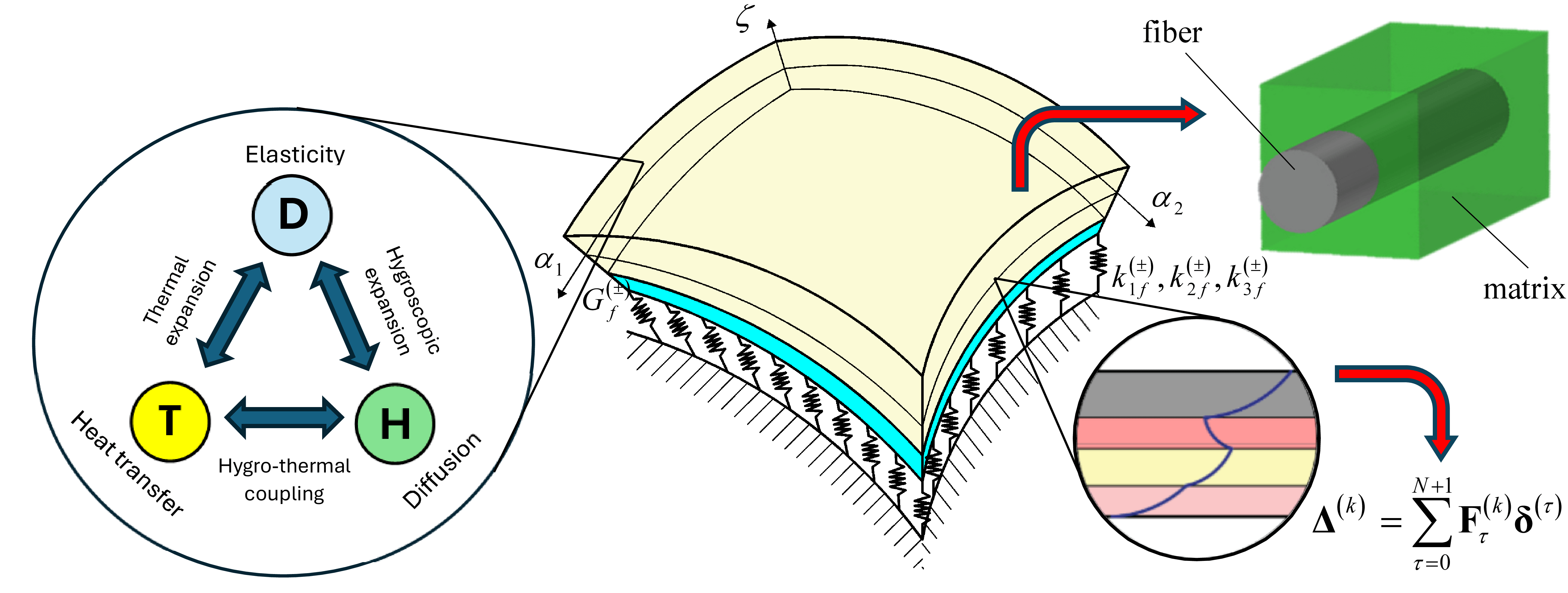
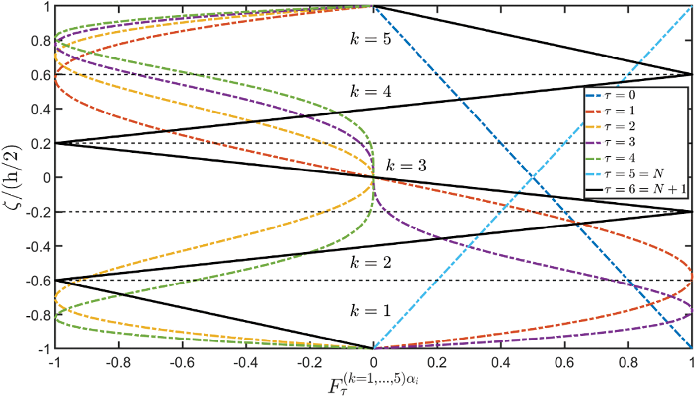
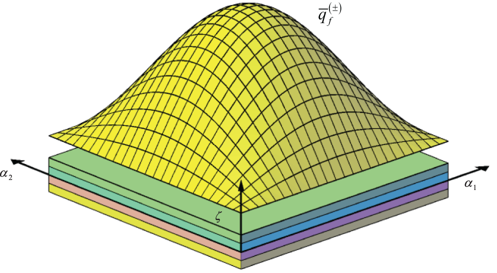
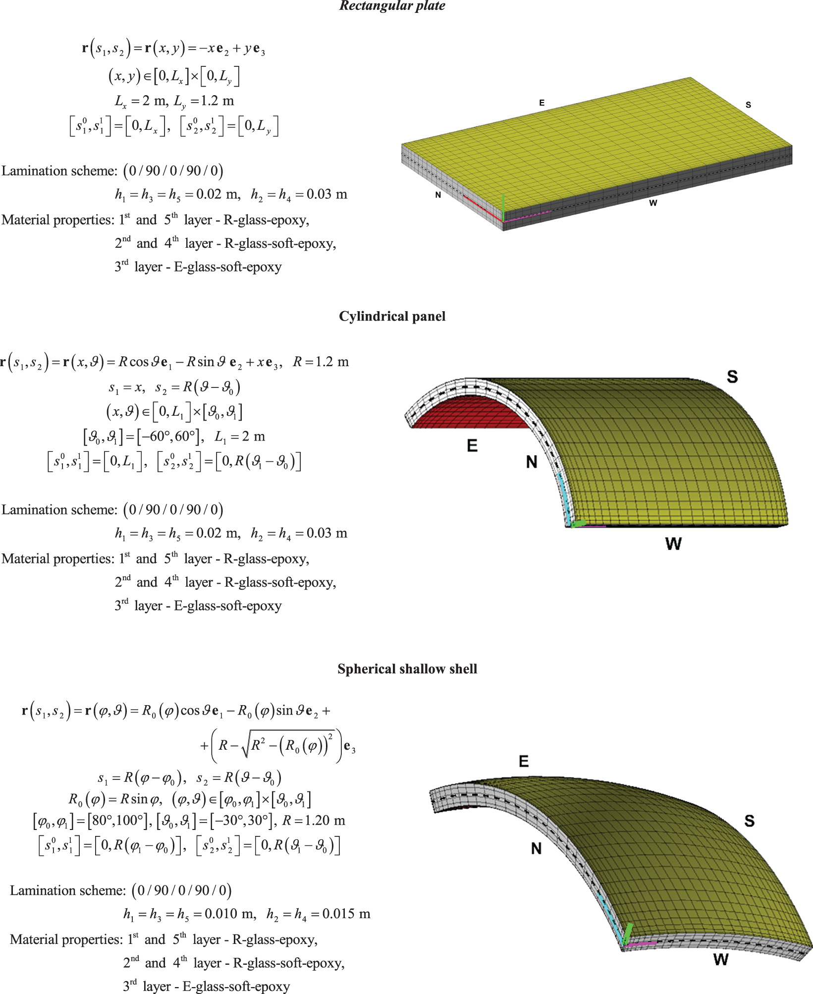
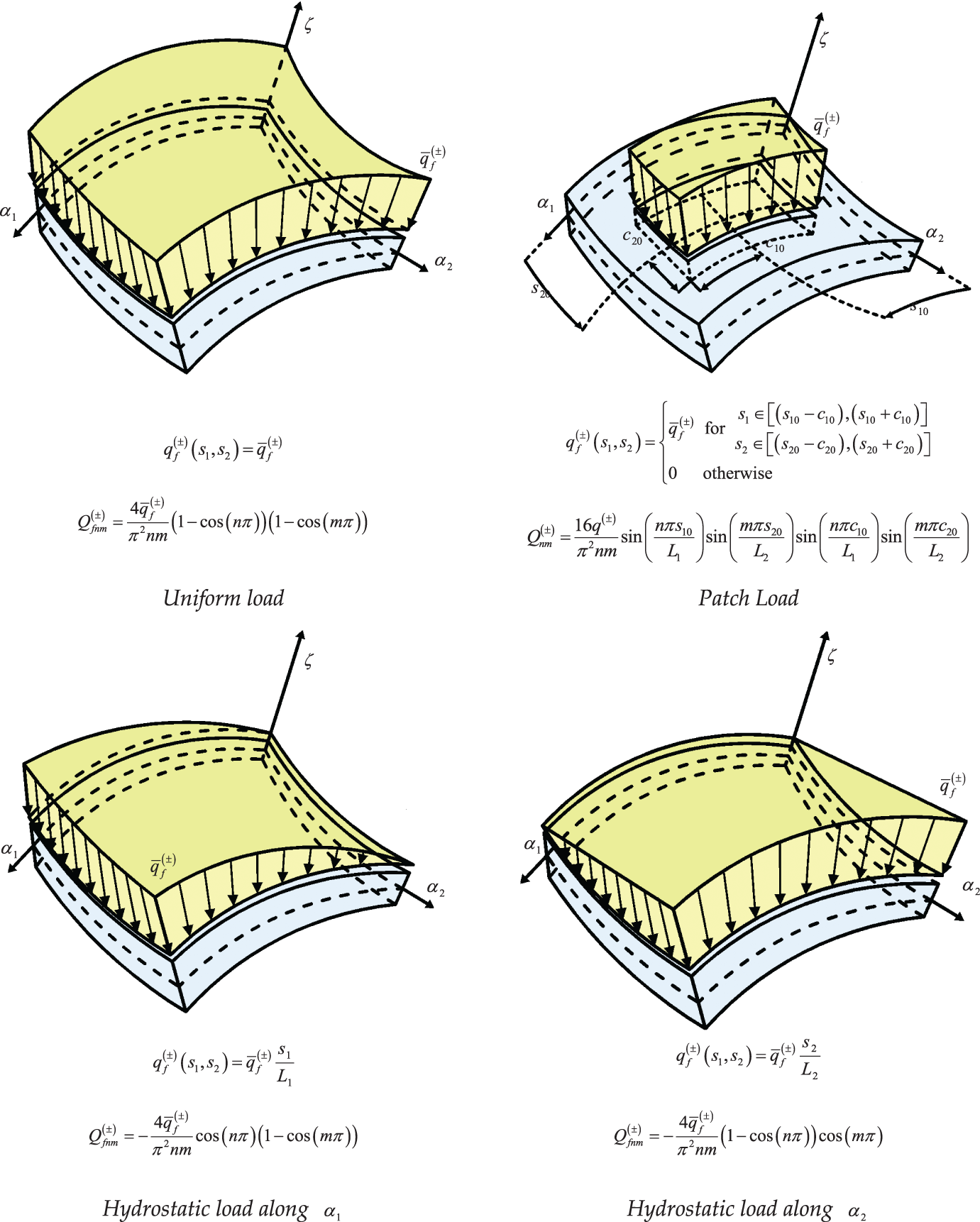
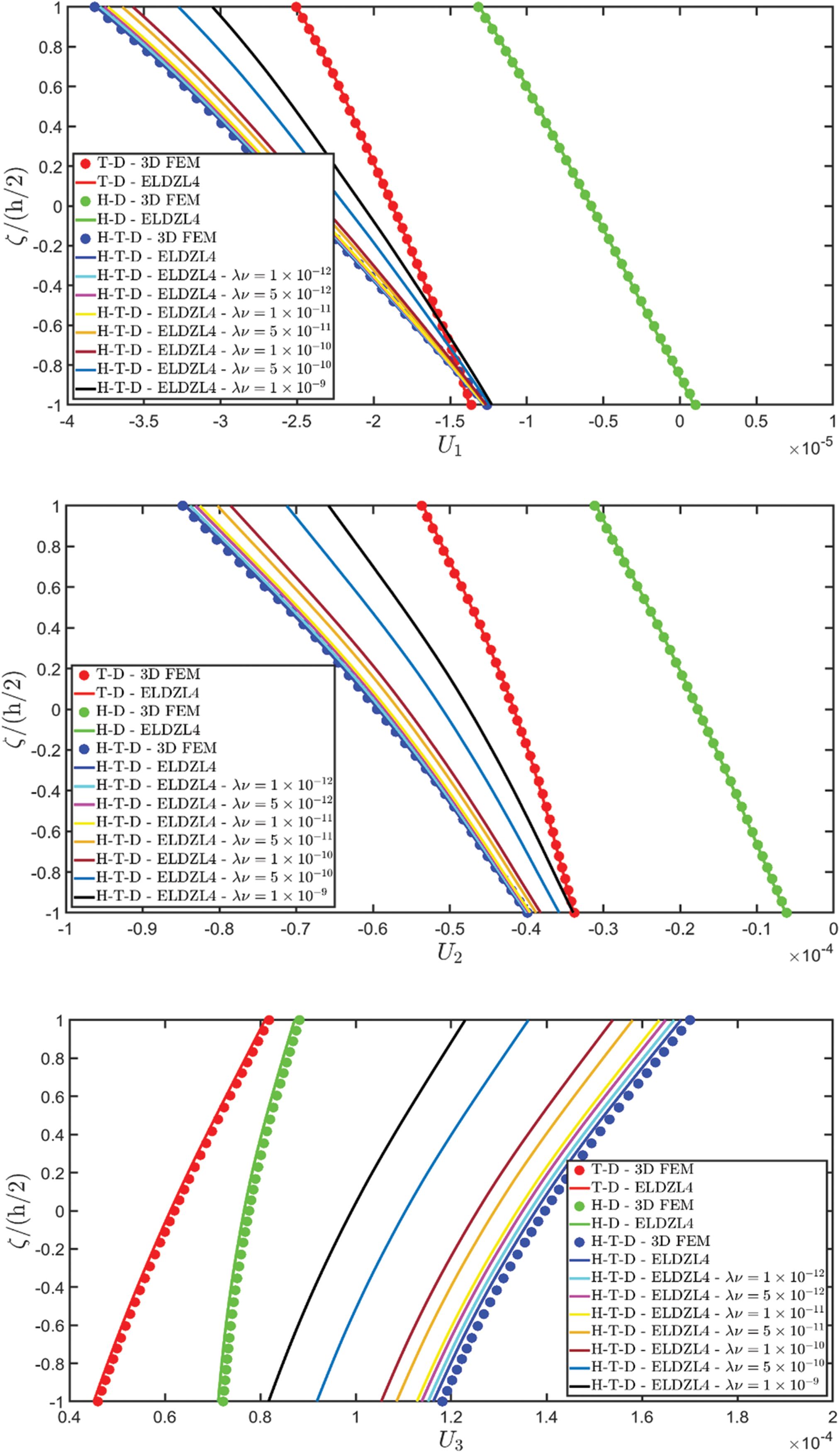
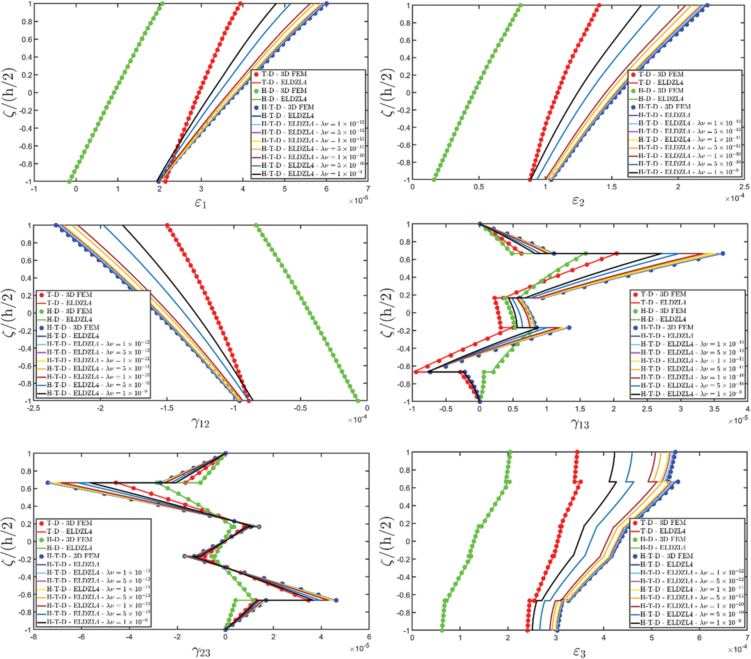

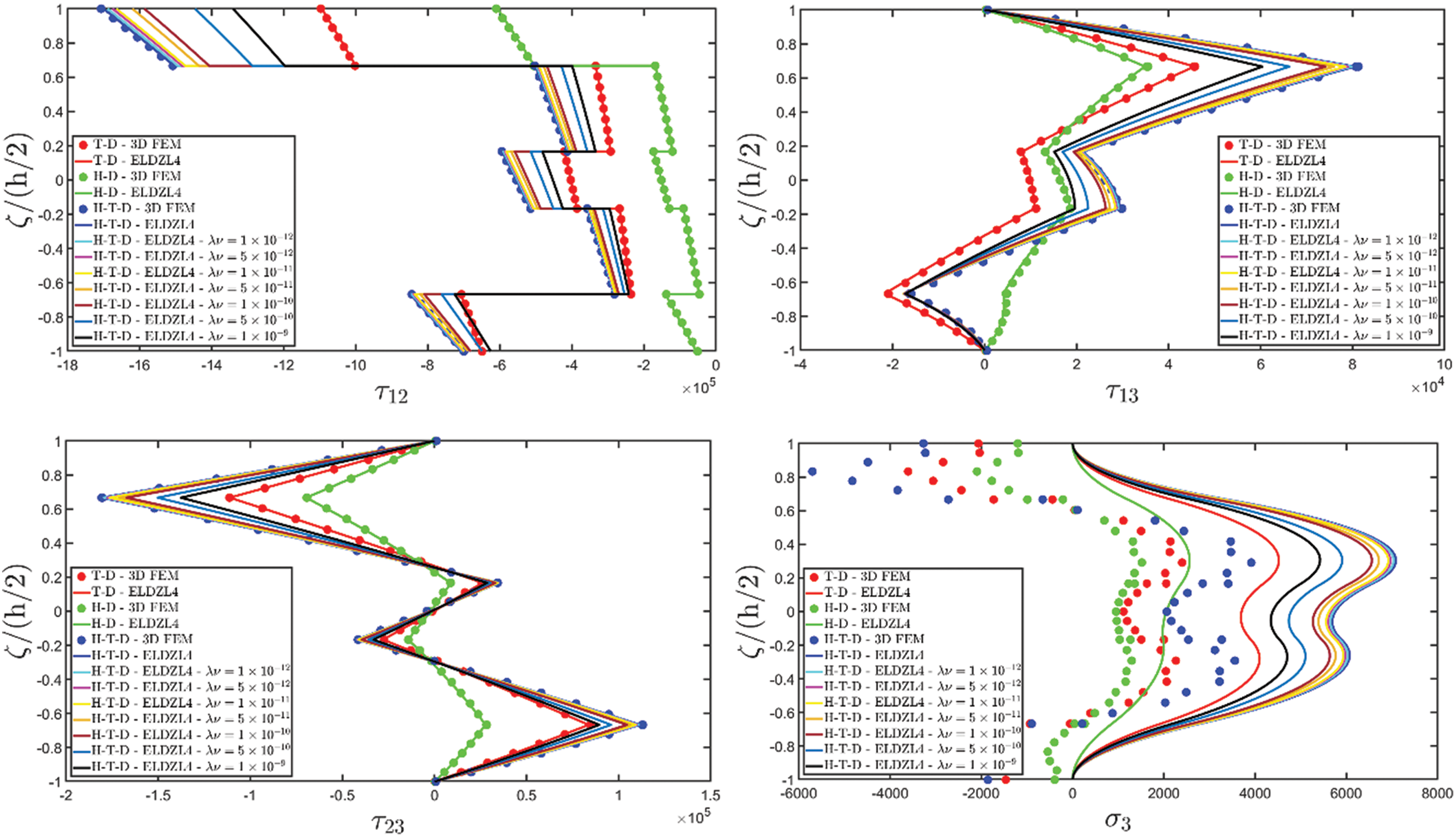
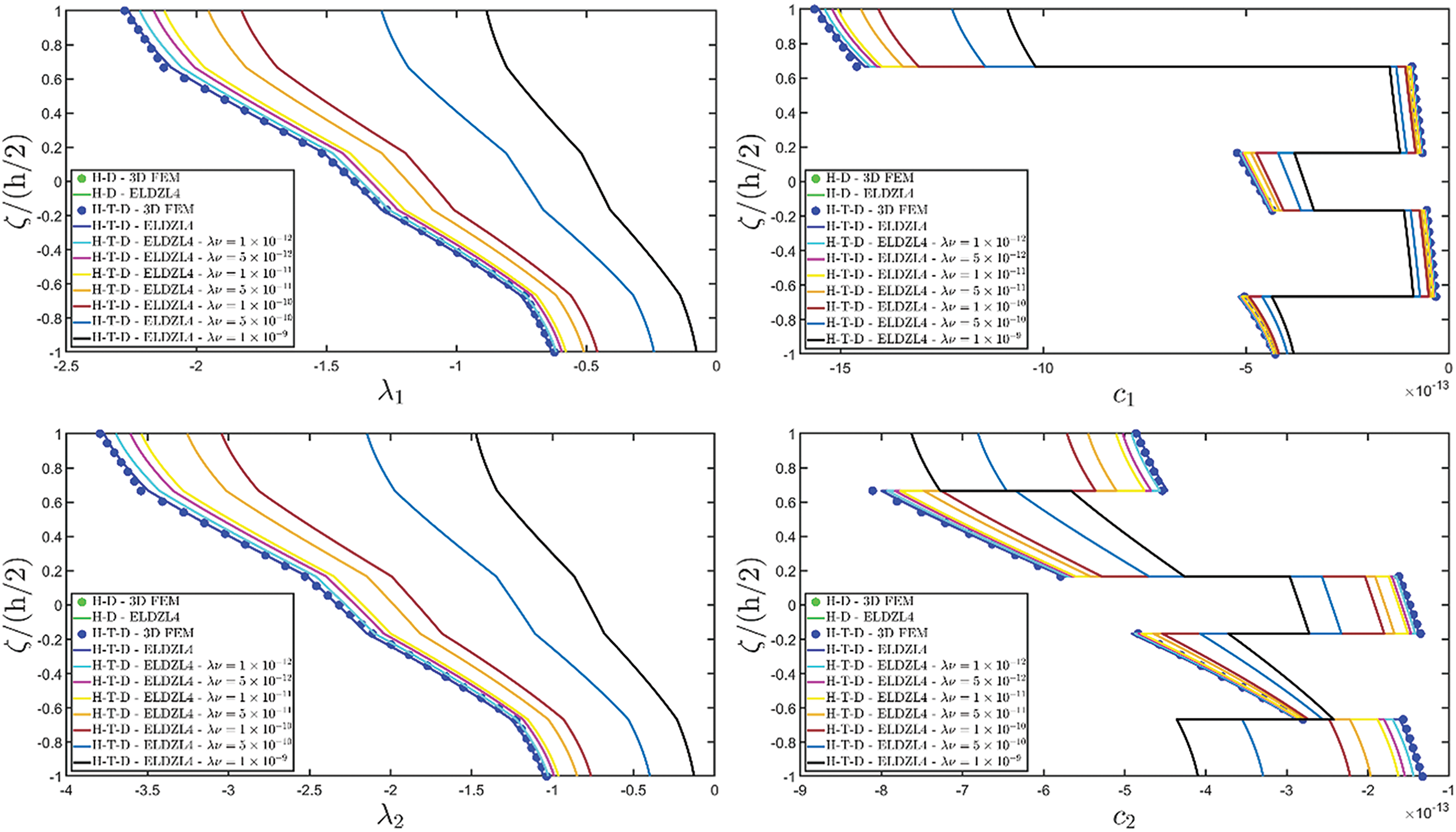
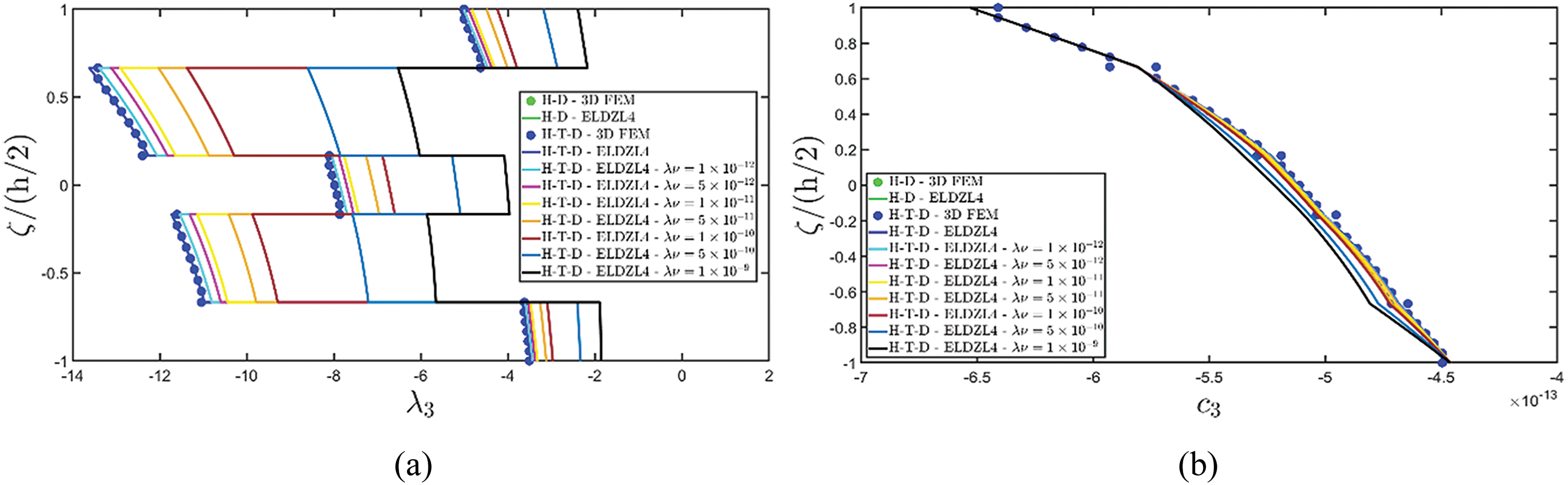
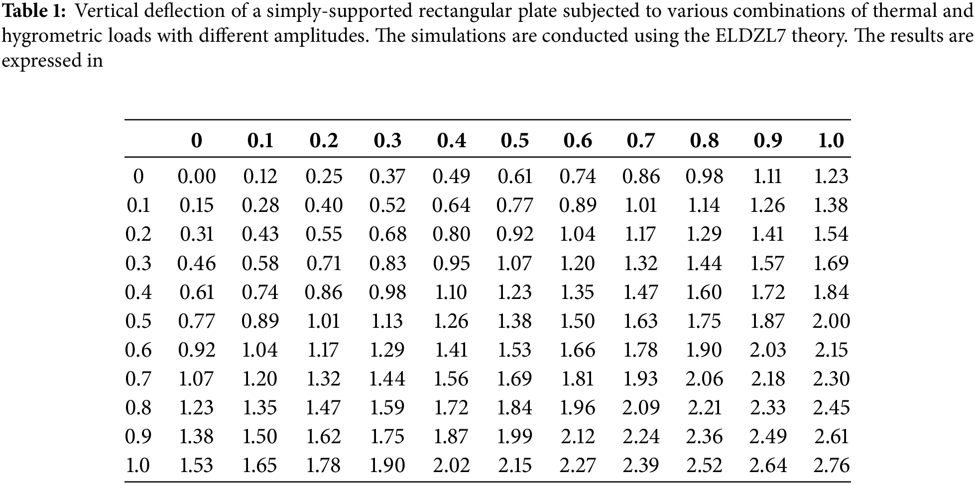
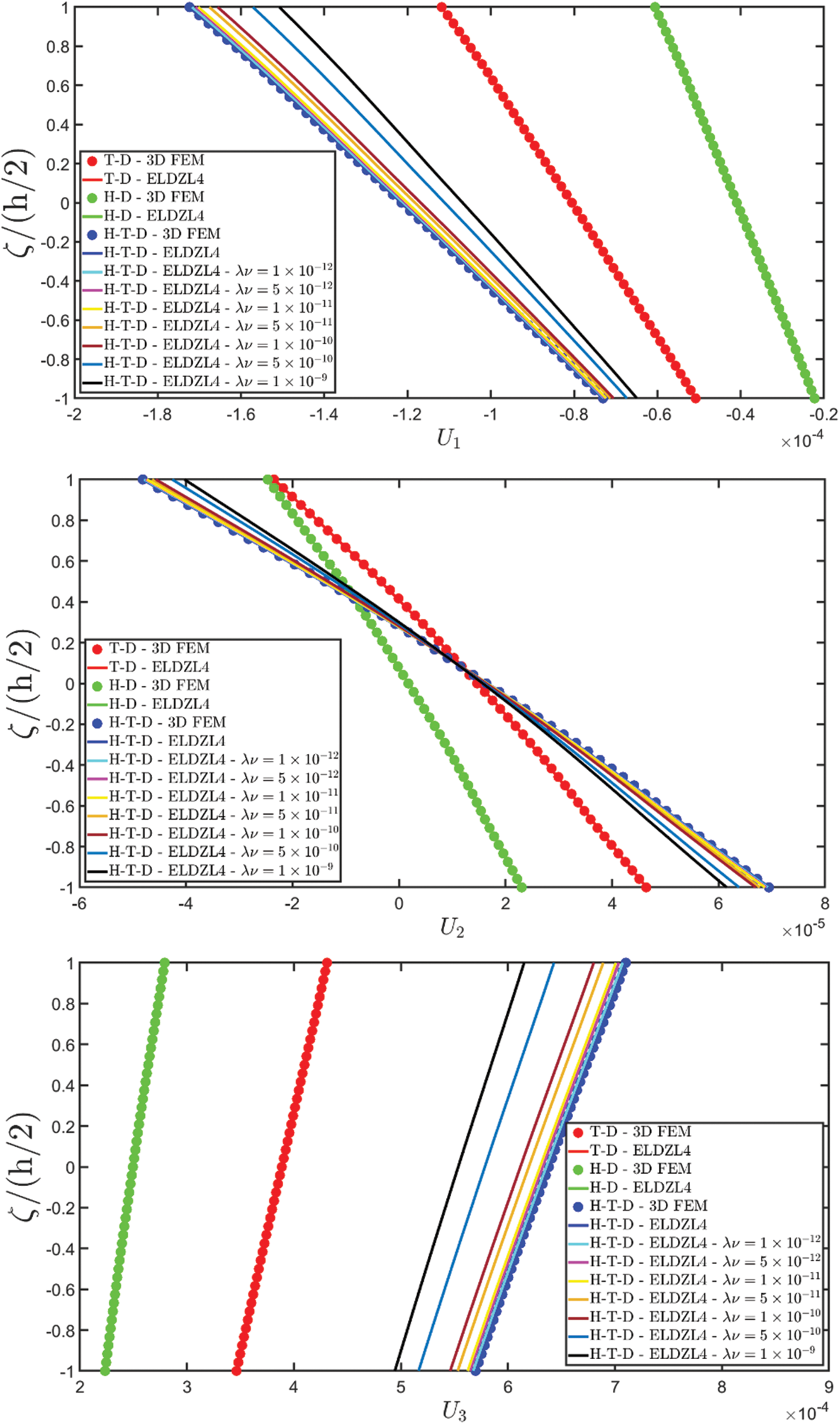
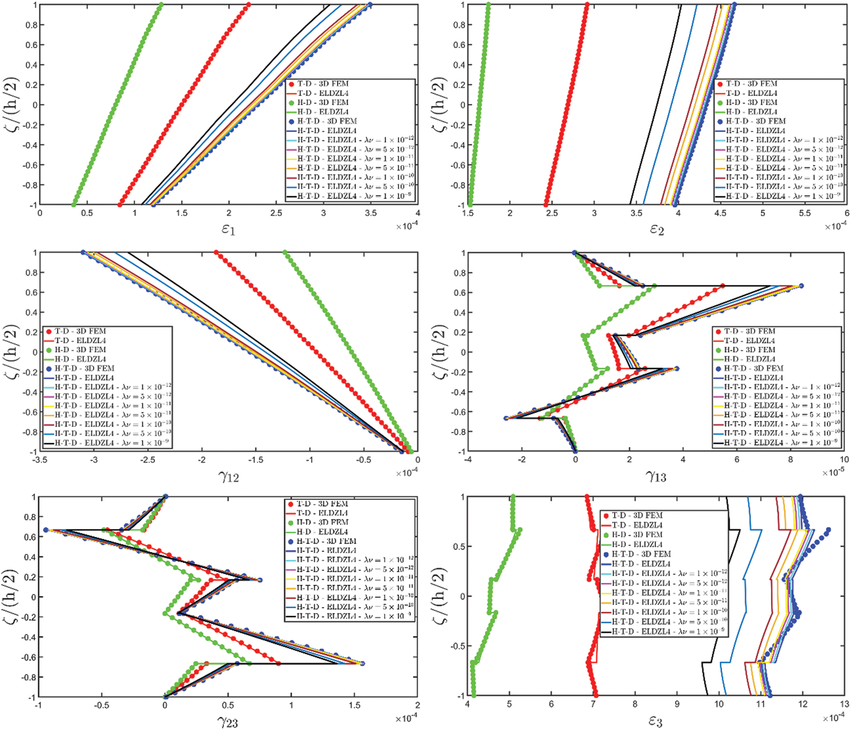
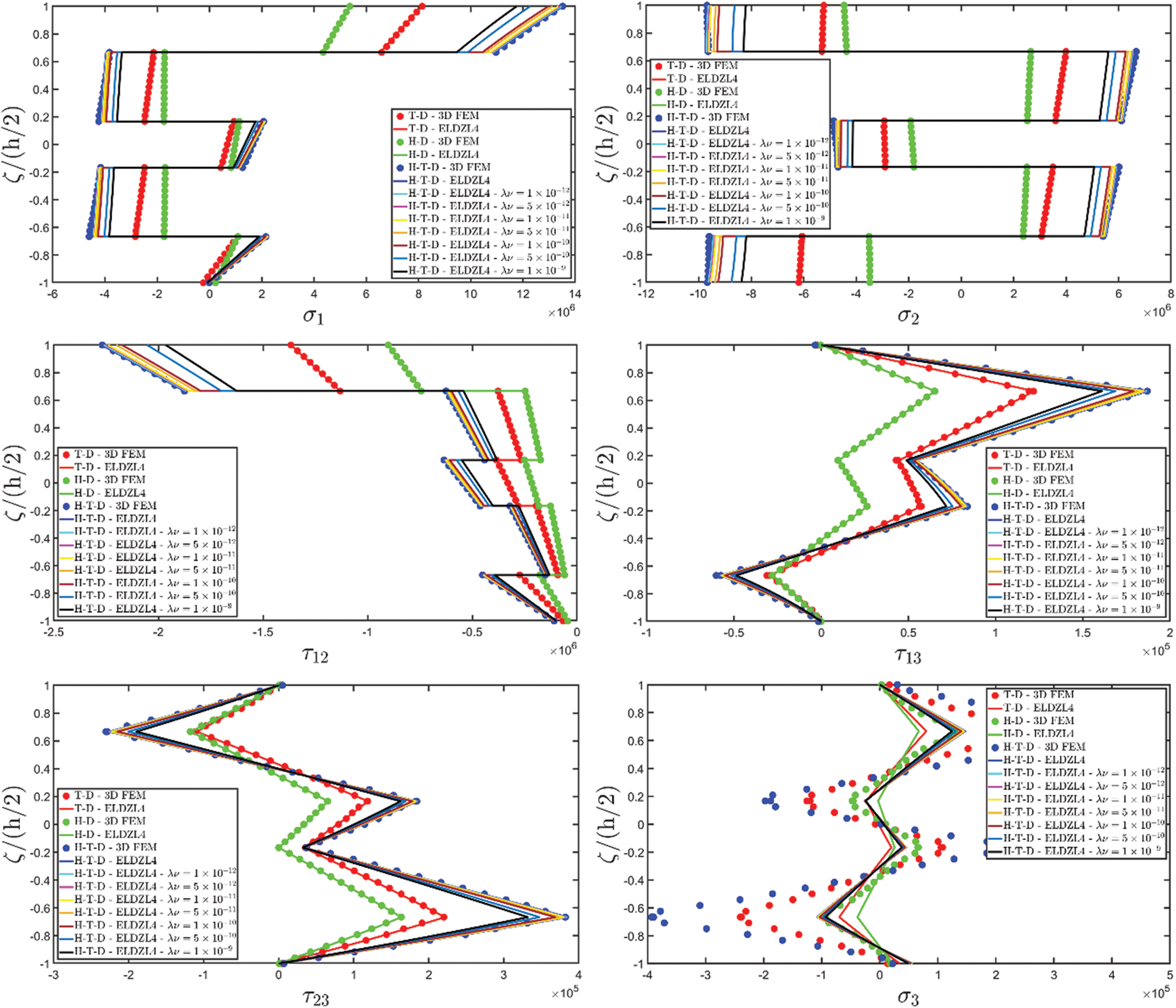
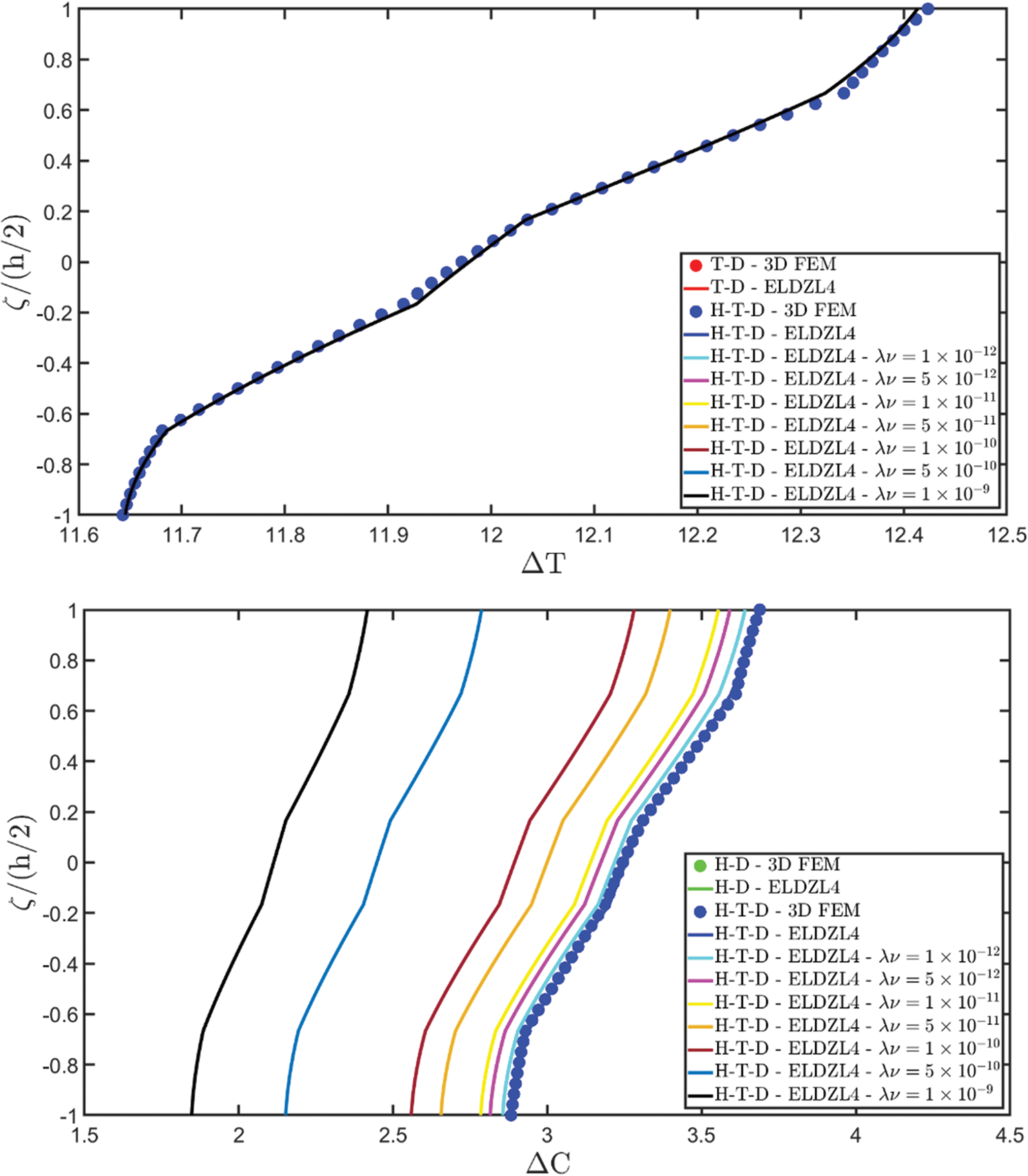
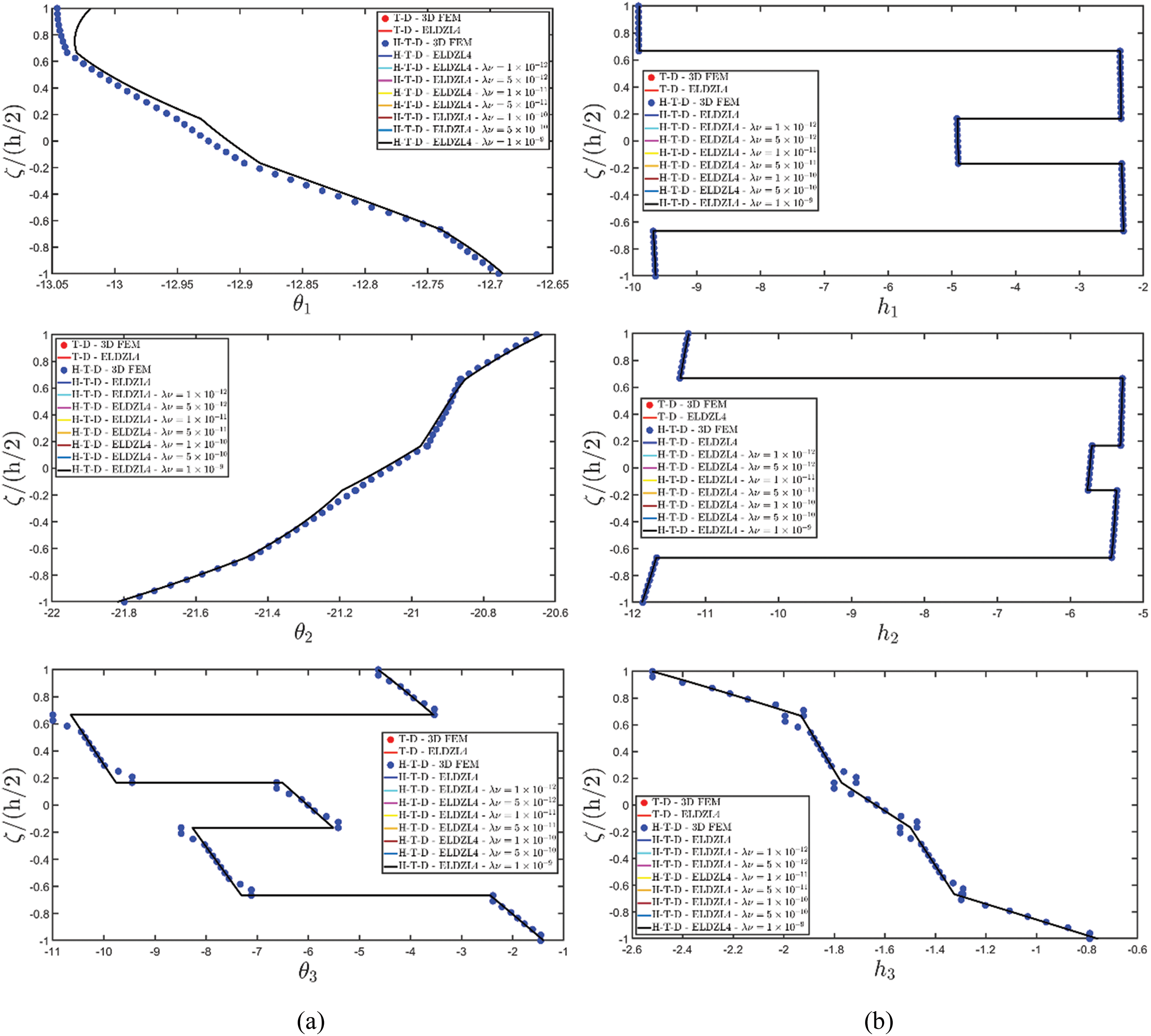
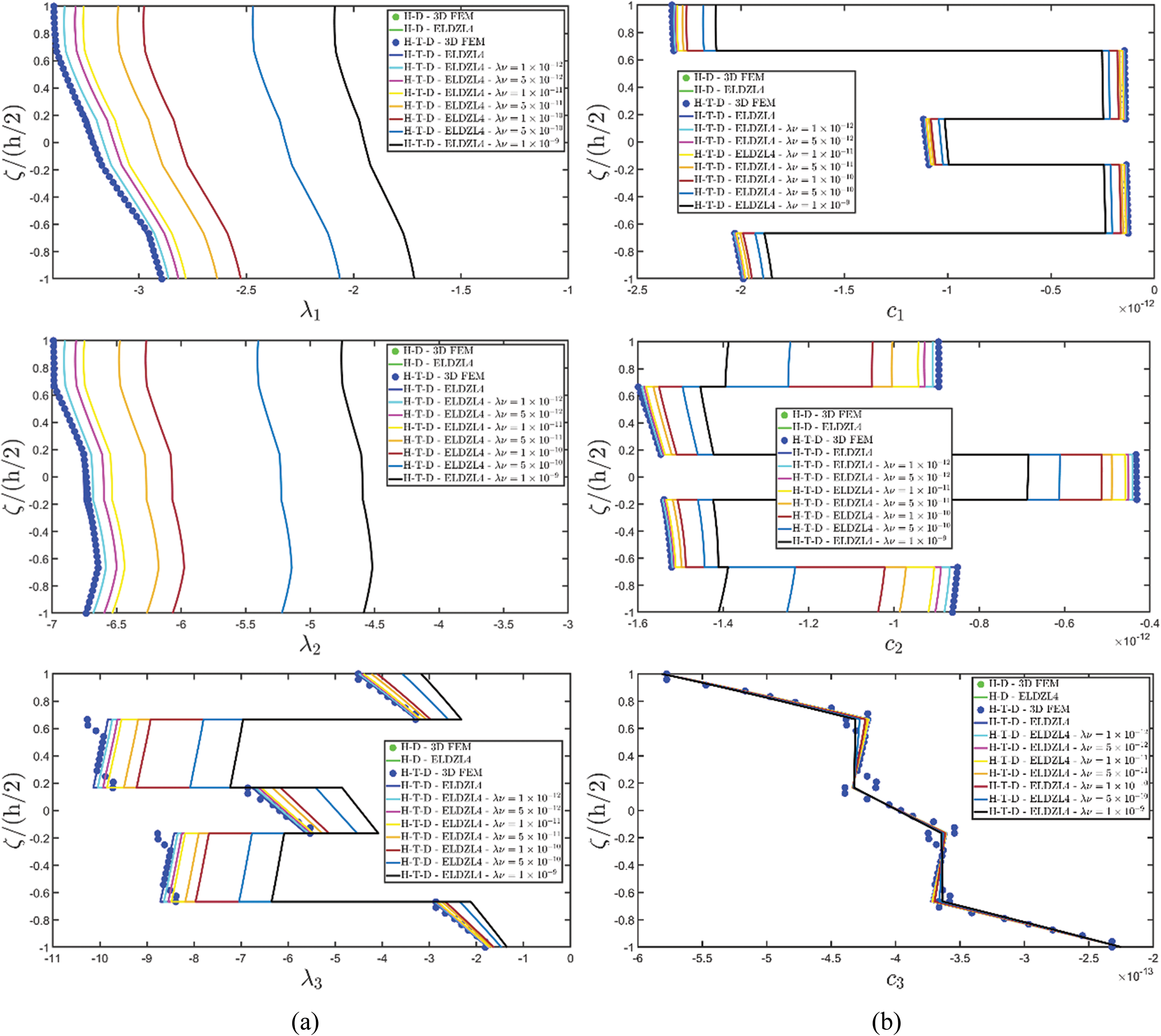
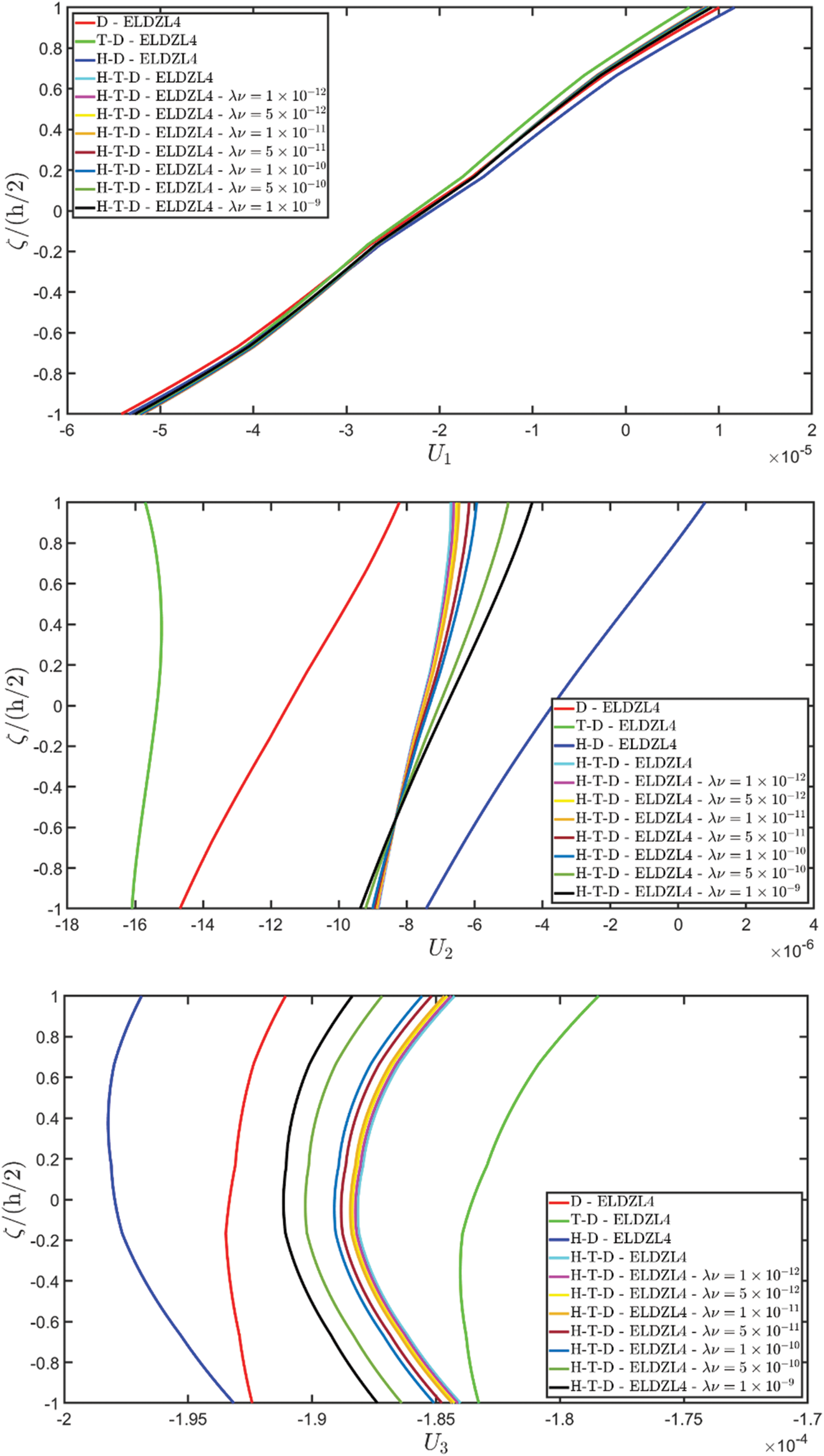
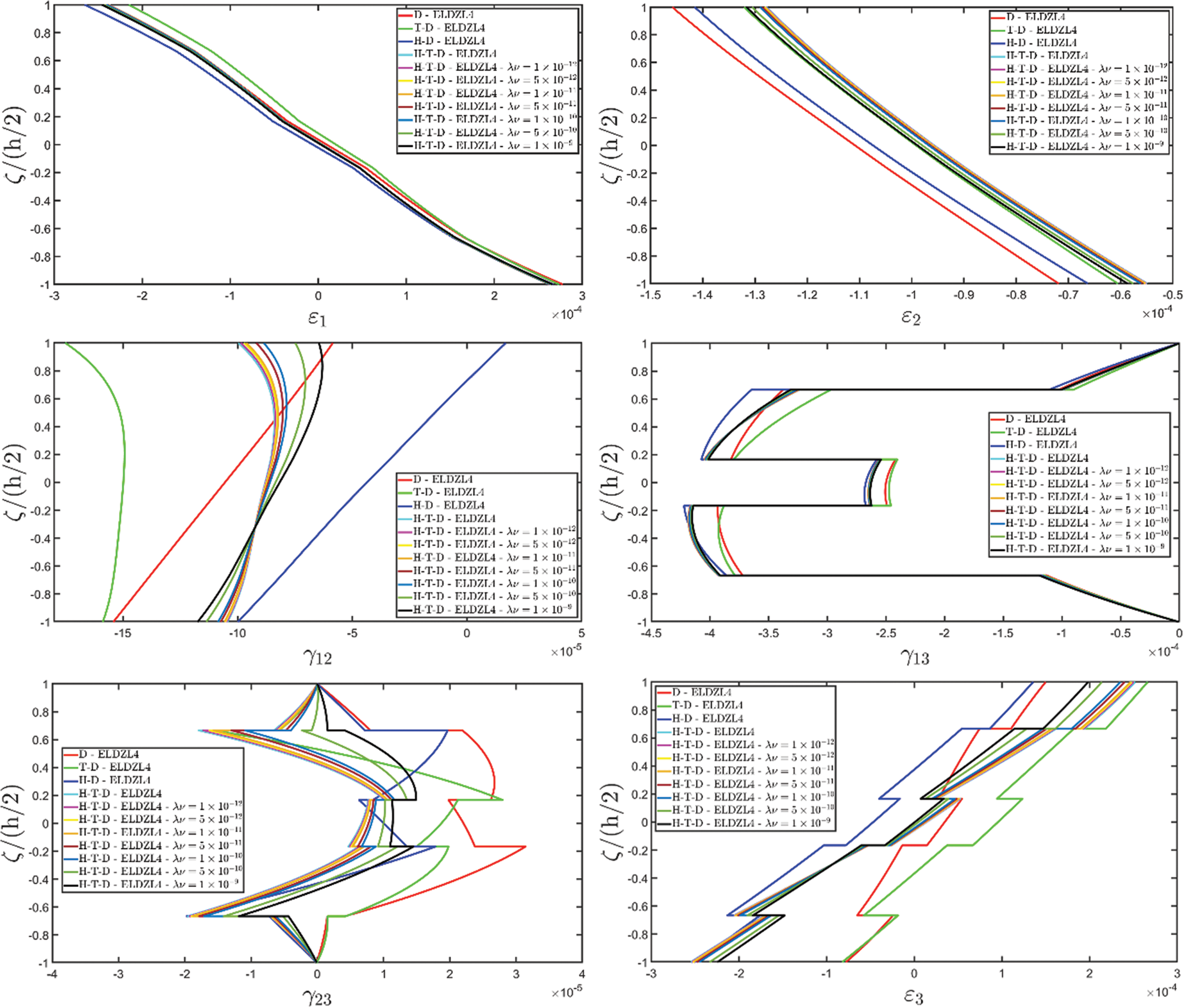
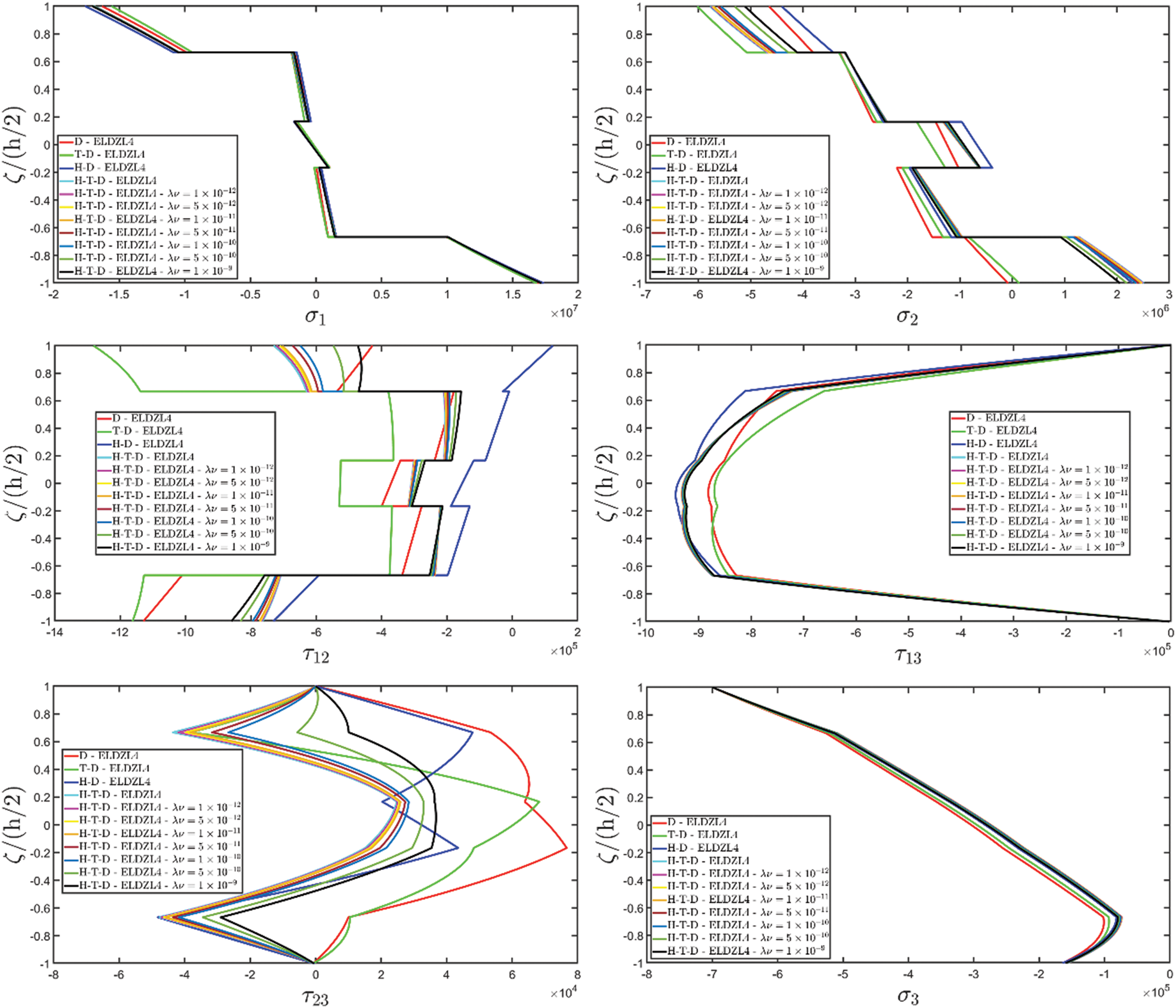
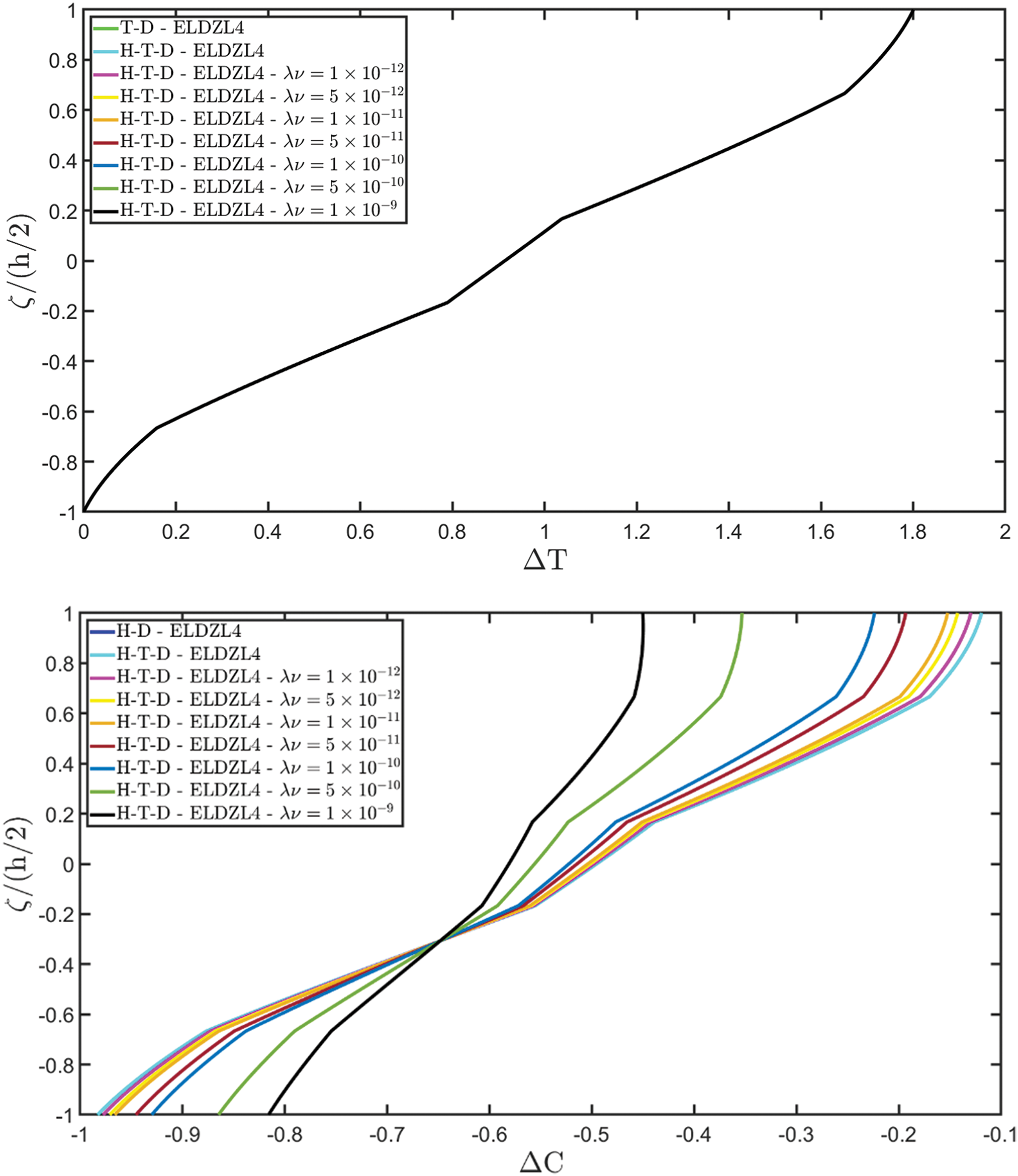
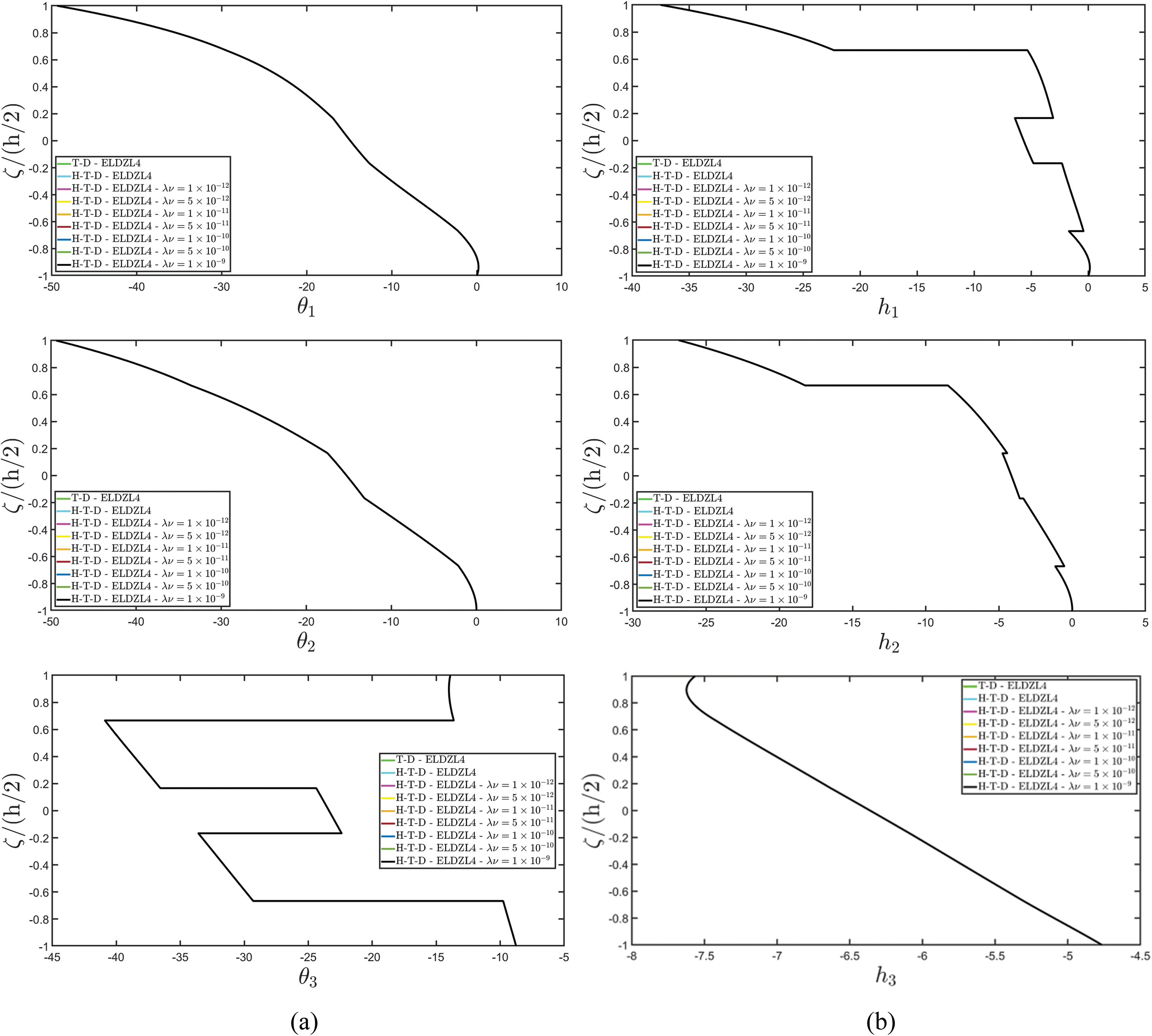
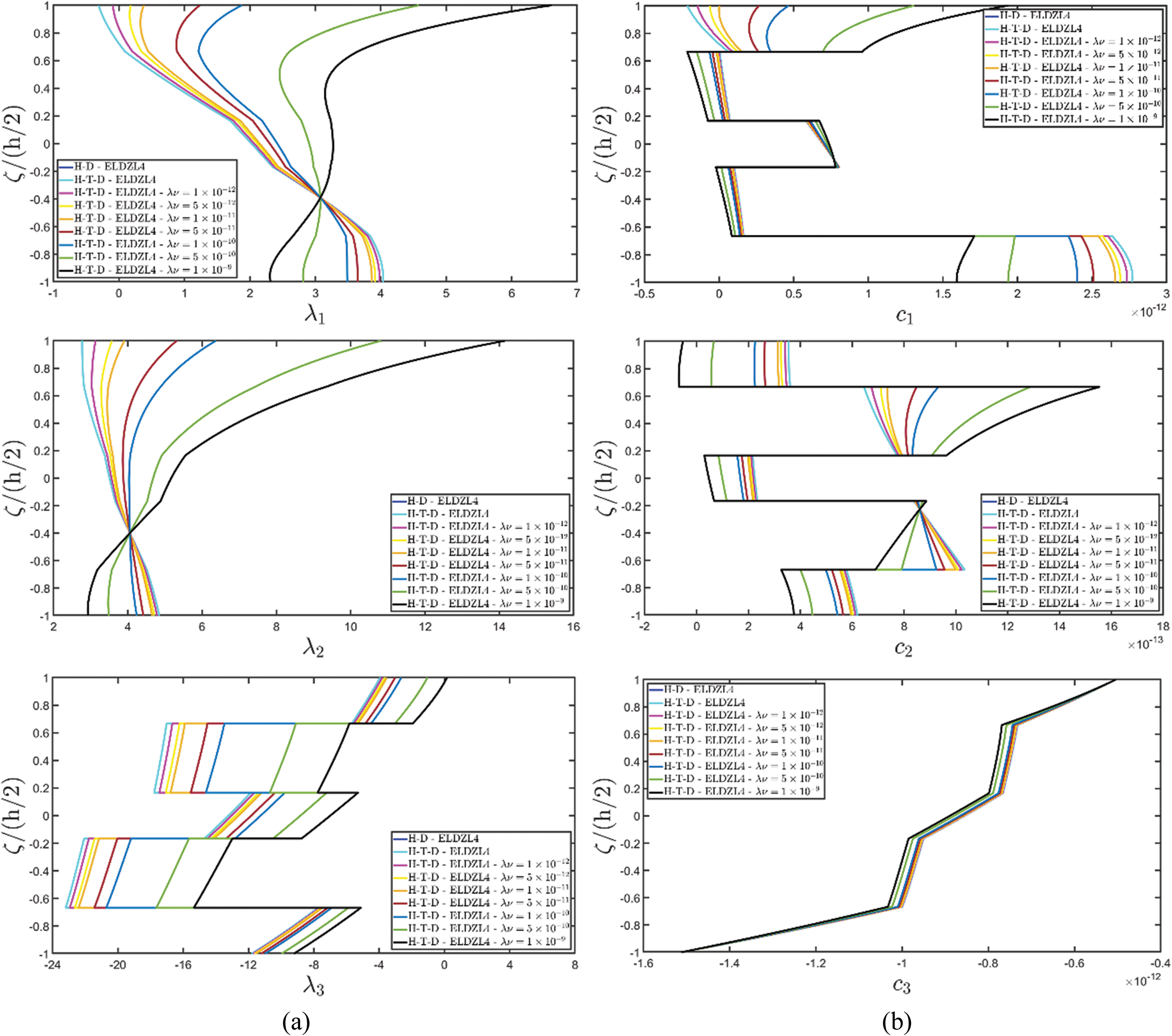
 Copyright © 2025 The Author(s). Published by Tech Science Press.
 Downloads
 Citation Tools