1 Introduction
Recent advancements in many engineering applications adopt smart materials [1] that can respond to external actions and environmental conditions, depending on design requirements. In this context, structural components characterized by either sensor or actuator functions become important [2–4]. In literature, there is increased attention to structural elements sensitive to environmental changes, known as smart structures, as demonstrated by the large applications in manufacturing industries involving smart composites, such as sensors, actuators, and energy harvesting systems [5–7]. These smart materials are characterized by a high stiffness-to-weight ratio similar to traditional heterogeneous composites, typically consisting of an isotropic medium reinforced by short or long fibers. Moreover, piezoelectric phases are increasingly used in composite applications due to their high mechanical stiffness and ability to respond to electric fields [8,9]. When considering a smart composite material, the interaction between the constituent phases likely produces a field coupling not present in each phase. More specifically, combining a piezoelectric material and a component with an elevated thermal expansion coefficient can generate pyroelectricity in the overall composite [10,11]. Similarly, combining a piezoelectric phase with a piezomagnetic material has been shown to produce a magnetoelectric coupling effect [12–15]. This means that in magnetoelectric composites, an external magnetic field can induce an electric field within the solid, and, conversely, an external electric field may produce a magnetic response. Among the literature, increased interest has been recently observed on multifield effects [16], caused by a product tensor property [17]. Starting from the most studied connectivity schemes such as particulate composite, laminate composite, and fiber composite [18], several sensor technical applications have been derived, including Alternating Current (AC) and Direct Current (DC) magnetic field sensors, magneto-electric current sensors, transformers, and gyrators, as well as tunable devices, magneto-electric filters, and phase shifters, among others [19–21].
Numerous studies address the experimental characterization and numerical investigation of magnetoelectric composites made of barium titanate and cobalt ferrite [22–25]. Analyzing the magneto-electro-composites requires both analytical and numerical methods to predict their multifield constitutive properties. This prediction is based on the constitutive equations for each phase of the heterogeneous material, where the geometric configuration of the Reference Volume Element (RVE) is derived in References [26–28]. In practical applications, magneto-electro-elastic composite materials frequently consist of fibrous and laminated composites. To this end, Reference [29] provides an analytical expression for the homogenized properties of magneto-electro-elastic materials, which are modeled with transversely isotropic symmetry. This homogenization technique is derived from the well-known Mori & Tanaka mean field approach [30].
Among the literature, several papers applied various formulations focusing on structures made of magneto-electro-elastic materials. In this way, it is possible to easily investigate the multifield response of smart materials under external static loads. For instance, a three-dimensional (3D) solution has been derived in Reference [31] for the static analysis of functionally graded magneto-electro-elastic plates, taking into account an exponential variation in the material properties along the thickness direction. In the same way, Reference [32] provides an analytical study of magneto-elastic rotating cylinders in a thermal environment characterized by a power-law variation of the material properties along the radial direction. Finally, in Reference [33], a two-dimensional (2D) analytical model is provided for the study of magneto-electro-elastic cantilever beam structural elements with rectangular cross-sections. In all these papers, when the magneto-electric effect is not ignored, additional terms must be included in the computation of the system’s total energy, to account for the coupling effect of these fields. This reverts to a fully coupled theoretical model, where the fundamental governing equations of each physical problem are solved simultaneously [34–38]. On the other hand, to obtain an analytical solution, several simplifications must be introduced within the model. For this reason, approximate numerical results are preferred for practical applications. When a classical Finite Element Method (FEM) is adopted, the results may be less accurate, especially with linear triangular and hexahedral discretizations. As a result, a Smoother FEM (S-FEM) in its Cell-based S-FEM (CS-FEM) and Edge-based S-EEM (ES-FEM) can be introduced in 3D and 2D problems to overcome such limitations. For multifield simulations, the Coupled multifield CS-FEM methodology is adopted for accurate results, as shown in References [39,40].
A theoretical formulation with coupled physics can be highly demanding from a computational standpoint when deriving a numerical solution, due to the high number of Degrees of Freedom (DOFs) involved. Such complexity, however, can be overcome by using refined 2D solutions instead of 3D formulations. For instance, in Reference [41], a refined higher-order theory is adopted for magneto-electro-elastic cross-ply shell structures in a hygro-thermal environment, while in Reference [42] a 2D formulation has been provided to investigate the mechanical response of laminated curved panels in a thermal environment under prescribed thermal flux and temperature values. Finally, in Reference [43], the mechanical problem of generally anisotropic shell structures with variable thickness is investigated through refined 2D theories.
Among 2D theories, two different methodologies are commonly employed: the Layer-Wise (LW) approach and the Equivalent Single Layer (ESL) approach. According to LW, the fundamental equations are solved within each layer of laminated structures, with the unknown DOFs distributed along the thickness direction. On the other hand, in ESL problems, the governing equations are solved for the entire structure, and the DOFs are located on the reference surface at the mid-thickness of the solid [44–46]. In addition to ESL and LW, the Equivalent Layer-Wise (ELW) approach [47,48] is a hybrid method that combines the ESL expansion of unknown variables along the thickness direction [49] with the polynomials used in LW theories [50]. As a consequence, ELW theory can be viewed as a particular case of ESL theories, allowing to prescribe arbitrary values for the configuration variables at the top and bottom surfaces of the panel. This approach enables the solution of mechanical elasticity equations and electrostatic or magnetostatic problems within the same model, without any restriction on the through-the-thickness distribution of both electrostatic and magnetostatic potentials. This aspect is crucial for thick structures, where the profile of the electrostatic potential depends on the stacking sequence [51–53]. On the other hand, in the case of thin structures, a linear profile provides sufficiently accurate numerical predictions [54,55]. In ESL, LW, and ELW theories, the accuracy of the solution depends on the selection of the expansion for the configuration variables along the thickness direction. A significant milestone in this field is the generalized formulation proposed for the first time in the pioneering research by Washizu [56] and Reddy [57], which enables an arbitrary through-the-thickness expansion of the unknown field. This generalized theory is, thus, derived regardless of the specific expression of the selected thickness function, embedding various theories in a unified manner [58], including classical approaches like the Classical Plate Theory (CPT), the First Order Shear Deformation Theory (FSDT) and the Third Order Shear Deformation Theory (TSDT) [59]. In ESL and ELW theories, the interaction between adjacent laminae is modeled using zigzag functions [60]. The pioneering work by Murakami [61] provides a straightforward evaluation of the zigzag effect based on the slope variation of the thickness function at each interface. On the other hand, the refined zigzag theory [62–64] derives the thickness function from the mechanical properties of the stacking sequence of the structure. However, this theory is primarily suitable for classical composite materials. As a consequence, various papers can be found in the literature that explore various analytical expressions for the kinematic model, from trigonometric [65,66] to polynomial [67–70] functions. In the case of structures with very complex shapes, the thickness function set can depend, also, on the geometry parameters of the structure [71]. As a consequence, an accurate methodology must be adopted to describe the geometry of the structure. To this end, several works employ the main results of differential geometry [72–75]. It has been shown in various papers that the most efficient methodology for describing the geometry of a doubly-curved shell involves its parametrization with curvilinear principal coordinates [76,77]. This approach facilitates the definition of the fundamental equations of a structural problem. However, for arbitrarily shaped structures, a coordinate change must be adopted through mapping procedures.
Closed-form analytical solutions of differential structural theories can be derived only for specific geometries, material symmetries, and boundary conditions, including clamped [78] and simply-supported [79–83], as happens for instance in the 3D theory proposed in References [84,85]. However, the reconstruction of the 3D configuration variables, as well as primary and secondary variables from the 2D semi-analytical solution, may be inaccurate because this formulation does not consider the equilibrium equations along the thickness direction. Therefore, in the post-processing stage, primary and secondary variables often require some adjustment. This requires a post-processing procedure that employs a numerical technique to solve 3D equilibrium equations starting from the solution derived from the 2D theory [86,87]. The computational demand of this procedure to yield accurate solutions can be high when using approaches like the FEM numerical technique, especially for lamination schemes with many layers [88–91]. For this reason, the Generalized Differential Quadrature (GDQ) is adopted frequently [92–94] in this context, because it allows for the use of a reduced number of sampling points for an efficient definition of numerical derivatives [95,96]. The GDQ method has been extensively applied to analyze laminated panels of various shapes and materials, including those with lattice and honeycomb cores [97,98], Variable Angle Tow composites, porous materials, and three-phase materials reinforced by Carbon Nanotubes [99], among others. The GDQ method approximates the derivatives using a quadrature rule, with Lagrangian interpolating polynomials as basis functions. The Taylor-based Differential Quadrature (TDQ) and Harmonic Differential Quadrature (HDQ) methods, instead, adopt Taylor’s series and Fourier’s series, respectively, as basis functions [100–102]. In addition, the Generalized Integral Quadrature (GIQ) [103] is a numerical technique that combines the fundamental integration theorem with the GDQ method, enabling an accurate evaluation of the integral of a function with a limited number of sampling points.
In this work, a novel higher-order ELW formulation is presented for laminated anisotropic magneto-electro-elastic shell structures with double curvatures. The geometry of the panel is described using differential geometry principles with principal coordinates. Displacement components, along with electrostatic and magnetostatic potentials, are expanded using higher-order polynomials. A specific set of basis functions is selected to enforce pre-determined values of configuration variables of the problem. The fundamental relations are derived for a stationary configuration of the total energy of the system, considered as a potential functional, accounting for the coupling effects between mechanical elasticity and electrostatic and magnetostatic equations. Furthermore, the formulation includes the magneto-electric coupling within the solid. A two-parameter elastic foundation, based on the Winkler-Pasternak theory, is modeled at the top and bottom surfaces of the panel. A semi-analytical Navier solution is derived for laminated panels with constant curvatures and cross-ply lamination schemes. Then, a post-processing technique is used to recover the primary and secondary variables from the 3D multifield balance equations, which are solved numerically using the GDQ method. Several examples are presented to validate the model against 3D finite-element-based numerical solutions, as developed in commercial codes. The results demonstrate that the proposed formulation yields highly accurate results with a reduced computational effort compared to highly demanding simulations, even for complex structures and loading conditions. Furthermore, the influence of the magneto-electric coupling within the model is investigated. This theory is demonstrated to be a valuable tool for exploring new design possibilities of magneto-electro-elastic components in various sustainable engineering applications. In this perspective, the elements of the novelty of this research rely on the computational efficiency of the theory while preserving the high accuracy level. The adoption of higher-order theories, indeed, allows for an efficient prediction of the 3D response of the structure despite the 2D nature of the theory. Furthermore, the description of the structure through differential geometry principles enables a generalized version of the magneto-electro-elastic theory which can be steadily applied to various geometries by simply adopting different values of the geometric parameters of the panel.
The refined 2D formulation presented in the paper is based on some assumptions regarding the lamination scheme, the geometry of the structure, and the kinematic assumption along the thickness direction. In particular, a generalized kinematic model is adopted for the description of the unknown field variables. Their through-the-thickness distributions are described by using arbitrary thickness functions, thus introducing generalized configuration variables for each order of kinematic expansion. In this way, the 3D solid is reduced to its reference surface, located at the middle thickness. A general shape of external surface loads is applied to the panels, which are simply supported at its four edges. The constitutive behavior of each lamina of the panel accounts for the full coupling between mechanical elasticity, electricity, and magnetostatics. More specifically, the constitutive relationship considers the direct and converse piezoelectric and piezomagnetic effects. Furthermore, additional coupling terms are introduced which couple electricity and magnetostatic equations. In this way, the multifield response can be easily derived not only for structures made of classical piezoelectric and piezomagnetic effects but also for panels with smart materials that exhibit the whole coupling between these physical phenomena.
2 Geometric Description of a Doubly-Curved Shell
The present theory starts with the geometric description of a laminated doubly-curved shell panel. Following the ESL approach, a reference surface is determined in the middle thickness of the solid. In this way, the position vector of an arbitrary point in the doubly-curved shell solid, denoted by R, can be derived from the following relation [48]:
R(α1,α2,ζ)=r(α1,α2)+h(α1,α2)2zn(α1,α2)(1)
The previous equation, r(α1,α2) represents the position vector of the reference surface. This vector is expressed in terms of curvilinear principal coordinates αi=α1,α2, defined in the closed interval [αi0,αi1], with αi0<αi1. The dependence on the thickness coordinate ζ is expressed in terms of the dimensionless quantity z=2ζ/h, where h is the total thickness of the shell for an arbitrary point located at (α1,α2) within the rectangular physical domain [α10,α11]×[α20,α21]. Furthermore, the outward unit vector n(α1,α2) is evaluated as follows [48], setting r,i=∂r/∂αi with i=1,2 the partial derivatives of the reference surface equation with respect to the principal coordinates α1,α2:
n(α1,α2)=r,1∧r,2|r,1∧r,2|(2)
In the same way, the principal radii of curvature Ri=R1,R2 along α1 and α2, respectively, can be evaluated as follows, setting r,ij=∂2r/(∂αi∂αj) the second-order derivative of the reference surface equation with respect to αi,αj with i,j=1,2 [48]:
Ri(α1,α2)=−r,i⋅r,ir,ii⋅n(3)
The reference surface of the shell is characterized by the Lamè parameters Ai=A1,A2, defined according to the following equation:
Ai(α1,α2)=r,i⋅r,i(4)
Finally, the curvilinear variation dsi=ds1,ds2 of a parametric line of the reference surface is related to the infinitesimal variation of principal coordinates dαi=dα1,dα2 as follows:
dsi=Aidαi(5)
where si∈[0,Li], and Li denotes the total length of the rectangular physical domain along the αi principal direction. In some cases, it is possible to derive a simple form of the integral version of Eq. (5). More specifically, it is assumed that the Lamé parameters Ai=A1,A2, in Eq. (4), and the principal radii of curvature Ri=R1,R2 of Eq. (3), assume a uniform value throughout the entire physical domain. In other words, their derivatives of the (n+m)-th order along α1,α2 or equivalently s1,s2 assume a null value:
A1=cost⇒∂n+mA1∂s1n∂s2m=0,A2=cost⇒∂n+mA2∂s1n∂s2m=0,
R1=cost⇒∂n+mR1∂s1n∂s2m=0,R2=cost⇒∂n+mR2∂s1n∂s2m=0(6)
As a consequence, the lengths L1 and L2 of the parametric curves along the α1 and α2 principal directions are calculated from the following relations:
L1=s11−s10=(α11−α10)R1L2=s21−s20=(α21−α20)R2(7)
where α10,α11 and α20,α21 denote the extremities, along α1 and α2, of the rectangular physical domain, respectively, while the quantities s10,s11 and s20,s21 are defined as sij=αijRi with i=1,2 and j=0,1. In case of a cylinder obtained from the translation of a circumference with generatrix corresponding to the α2 axis, the relations R1=+∞ and R2=R are assumed. As a consequence, the quantities L1,L2 are evaluated as follows:
L1=s11−s10=α11−α10L2=s21−s20=(α21−α20)R(8)
On the other hand, if the generatrix is assumed to be the α1 axis, one gets:
L1=s11−s10=(α11−α10)RL2=s21−s20=α21−α20(9)
Finally, in the case of a rectangular plate, the principal radii assume an infinite value, namely R1=+∞ and R2=+∞, therefore it gives:
L1=s11−s10=α11−α10L2=s21−s20=α21−α20(10)
As far as the thickness direction is concerned, a doubly-curved shell solid can be characterized, moving from Eq. (3), by means of the geometric scaling parameters Hi with i=1,2, which are defined at each point of the 3D solid, namely Hi(α1,α2,ζ)=1+ζ/Ri. When ζ=1, one gets Hi=1. Recalling that the structure is obtained from the superimposition of l laminae, the total thickness h(α1,α2) can be calculated as the sum of the thickness hk of each k-th lamina of the stacking sequence with k=1,…,l, leading to the relation reported below, derived from more general theoretical remarks reported in Reference [48]:
h(α1,α2)=∑k=1lhk(α1,α2)=∑k=1l(ζk+1−ζk)(11)
Here, ζk and ζk+1 denote the through-the-thickness location of the top and bottom surface, respectively, of an arbitrary k-th lamina of the lamination scheme.
3 Magneto-Electro-Elastic Definition Equations
In the present section, the vector Δ(k)(α1,α2,ζ) is introduced throughout the entire doubly-curved 3D solid for each k=1,…,l, which contains the configuration variables of the magneto-electro-elastic 3D formulation. These variables include the displacement field components U1(k),U2(k) and U3(k) with respect to the principal axes α1,α2,ζ, along with the variations of electrostatic and magnetostatic potentials Δϕ(k)=ϕ(k)−ϕ0 and Δψ(k)=ψ(k)−ψ0, respectively. Note that ϕ0 and ψ0 denote the values of these scalar quantities associated with the reference state of the solid, characterized by a stress-free condition. In particular, the vector Δ(k) assumes the following extended form:
Δ(k)(α1,α2,ζ)=[U1(k)U2(k)U3(k)ΔΦ(k)ΔΨ(k)]T(12)
In this work, the configuration variables of Eq. (12) are expressed according to the well-known International Standards (SI). Therefore, the displacement field components U1(k),U2(k),U3(k) are defined in meters (m), while the electrostatic potential is in volt (V). On the other hand, the magnetostatic potential is expressed in ampere (A). Following a generalized approach, the 3D configuration variables vector Δ(k) can be expressed in terms of generalized expansion of configuration variables defined in the 2D physical domain of the problem [48], collected in vector δ(τ)(α1,α2)=[u1(τ)u2(τ)u3(τ)ϕ(τ)ψ(τ)]T with τ=0,…,N+1:
Δ(k)=∑τ=0N+1Fτ(k)δ(τ)(13)
Employing an expanded notation, Eq. (13) can be expressed as:
[U1(k)U2(k)U3(k)Δϕ(k)Δψ(k)]=∑τ=0N+1[Fτ(k)α100000Fτ(k)α200000Fτ(k)α300000Fτ(k)α400000Fτ(k)α5][u1(τ)u2(τ)u3(τ)ϕ(τ)ψ(τ)](14)
The generalized expansion of Eqs. (13)–(14) is performed by means of the generalized thickness functions Fτ(k)αi=Fτ(k)αi(ζ) with i=1,…,5, defined for each τ=0,…,N+1 expansion order, depending on the thickness coordinate ζ. In this way, it is possible to derive a generalized formulation embedding various kinematic assumptions for the present multifield problem, including classical theories like CPT, FSDT and TSDT of the mechanical case. A different selection of thickness functions determines a different level of refinement in the model. In particular, refined models are obtained from Eq. (13) by selecting higher-order polynomials up to the N-th order. In addition, the term corresponding to τ=N+1 is associated with zigzag functions, facilitating an accurate and straightforward prediction of the interaction between adjacent laminae. Indeed, the zigzag functions induce an abrupt slope variation of the through-the-thickness profile of each configuration variable in the interlaminar region between an arbitrary k-th layer and the k+1-th lamina. The following relation is adopted for τ=N+1, setting i=1,…,5 [48]:
FN+1(k)αi(ζ)={(−1)kz⌢k=−ζ−ζ1ζ2−ζ1fork=1(−1)kzk=(−1)k(2ζ−ζkζk+1−ζk−1)fork=2,…,l−1(−1)kz⌣k=(−1)lζ−ζl+1ζl+1−ζlfork=l(15)
In line with the ELW approach [48], the following relations are adopted for τ=0,…,N, where z~=z∈[−1,1] is already defined in Eq. (1):
Fτ(k)αi(ζ)={1−z~2forτ=0z~τ+1−z~τ−1forτ=1,…,N−11+z~2forτ=N(16)
As observed in Eq. (16), the thickness functions assume a null value at ζ=h/2 and ζ=−h/2 when τ=1,…,N−1, while Fτ(k)αi=1 and Fτ(k)αi=0 at the bottom surface of the shell when τ=0 and τ=N, respectively. On the other hand, Fτ(k)αi=1 at the top surface for τ=N, while Fτ(k)αi=0 when τ=0. As a consequence, the arbitrary element δi(τ) of the vector Δ(τ) associated with τ=0 and τ=N+1 kinematic orders is equal to the corresponding element of the 3D vector Δ(k) of the configuration variables at the top and bottom surfaces, respectively [48]:
Δi(1)(α1,α2,ζ=−h2)=δi(0)(α1,α2)
Δi(l)(α1,α2,ζ=h2)=δi(N)(α1,α2)(17)
A proper nomenclature is adopted to denote the various kinematic models that can be employed in Eq. (14). More specifically, when the zigzag functions of Eq. (15) are used in the formulation, the acronym ELDZL−N is adopted, otherwise the kinematic model is described with the acronym ELD−N. Here, “EL” means that the kinematic model adopted in the theory follows the ELW approach, and “D” indicates that the unknown variables of the problem are the displacement field components, along with the electrostatic and the magnetostatic potentials. Finally, N is the maximum kinematic expansion order adopted in Eq. (13).
Moving from the ELW description of the unknown field variables, the definition equations are derived for the magneto-electro-elastic formulation in curvilinear principal coordinated. To this end, the vectors ε(k),E(k) and H(k) are introduced at each point of the 3D solid, with their extended form reported below:
ε(k)=[ε1(k)ε2(k)γ12(k)γ13(k)γ23(k)ε3(k)]T
E(k)=[ℰ1(k)ℰ2(k)ℰ3(k)]T
H(k)=[ℋ1(k)ℋ2(k)ℋ3(k)]T(18)
The vectors ε(k),E(k) and H(k) are conveniently arranged in vector π(k)=[ε(k)TE(k)TH(k)T]T of the primary variables of the magneto-electro-elastic formulation, defined at each point of the 3D solid. As a consequence, it is possible to provide a matrix form of the definition equations of the problem, as follows:
π(k)=DΔ(k)=DζDΩΔ(k)(19)
where D is a proper differential operator presented in detail in Reference [48]. As visible from the previous equation, this operator is split into two sub-operators Dζ and DΩ, accounting for the derivatives with respect to ζ and α1,α2, respectively. These operators can be written in an extended form according to the following relations:
Dζ=[Dζ(1)000Dζ(2)000Dζ(2)](20)
Here, the matrices Dζ(1) and Dζ(2) are defined as follows:
Dζ(1)=[1H10000000001H20000000001H11H20000000001H10∂∂ζ00000001H20∂∂ζ000000000∂∂ζ],Dζ(2)=[1H10001H2000∂∂ζ](21)
As far as the operator DΩ is concerned, the definition reported below can be introduced:
DΩ=[DΩ(1)000DΩ(2)000DΩ(2)](22)
where the sub-vectors DΩ(1) and DΩ(2) assume the following extended form [48]:
DΩ(1)=[D¯Ωα1D¯Ωα2D¯Ωα3]
DΩ(2)=[−1A1∂∂α1−1A2∂∂α2−1]T(23)
The quantities D¯Ωα1,D¯Ωα2,D¯Ωα3 introduced in the previous definitions can be expressed in curvilinear principal coordinates as:
D¯Ωα1=[1A1∂∂α11A1A2∂A2∂α1−1A1A2∂A1∂α21A2∂∂α2−1R10100]T
D¯Ωα2=[1A1A2∂A1∂α21A2∂∂α21A1∂∂α1−1A1A2∂A2∂α10−1R2010]T
D¯Ωα3=[1R11R2001A1∂∂α11A2∂∂α2001]T(24)
Finally, the differential operator DΩ is conveniently expressed as the sum of five different matrices, as follows:
DΩ=∑i=15DΩαi(25)
where the definition operators DΩαi with i=1,…,5 are reported below, setting D¯Ω(2)α4=D¯Ω(2)α5=DΩ(2):
DΩα1=[D¯Ωα100000000000000],DΩα2=[0D¯Ωα20000000000000],DΩα3=[00D¯Ωα3000000000000],
DΩα4=[00000000D¯Ωα4000000],DΩα5=[00000000000000D¯Ωα5](26)
In the generalized ELW setting, the 3D Eq. (19) are expressed by defining the configuration variables vector Δ(k) using the kinematic model of Eq. (13), i.e., [48]:
π(k)=DΔ(k)=DζDΩΔ(k)=Dζ∑i=15DΩαiΔ(k)=
=∑τ=0N+1∑i=15DζDΩαiFτ(k)Δ(τ)=∑τ=0N+1∑i=15DζFτ(k)αiDΩαiδ(τ)=∑τ=0N+1∑i=15Z(kτ)αiDΩαiδ(τ)=∑τ=0N+1∑i=15Z(kτ)αiπ(τ)αi(27)
In the previous equation, the vector π(k) has been expanded with the generalized primary variables vector π(τ)αi, introduced for each τ=0,…,N+1 and i=1,…,5. In other words, the following generalized definition equation is obtained:
π(k)=∑τ=0N+1∑i=15Z(kτ)αiπ(τ)αi⇔[ε(k)E(k)H(k)]=∑τ=0N+1∑i=15[Z1(kτ)αi000Z2(kτ)αi000Z2(kτ)αi][ε(τ)αiE(τ)αiH(τ)αi](28)
More specifically, the generalized vectors ε(τ)αi,E(τ)αi,H(τ)αi are introduced, accounting for the elasticity, electrostatic and magnetostatic definition equations in curvilinear principal coordinates. These vectors assume the following extended form [48]:
ε(τ)αi(α1,α2,t)=[ε1(τ)αiε2(τ)αiγ1(τ)αiγ2(τ)αiγ13(τ)αiγ23(τ)αiω13(τ)αiω23(τ)αiε3(τ)αi]T
E(τ)αi(α1,α2,t)=[ℰ1(τ)αiℰ2(τ)αiℰ3(τ)αi]T
H(τ)αi(α1,α2,t)=[ℋ1(τ)αiℋ2(τ)αiℋ3(τ)αi]T(29)
Finally, the ELW definition matrices Zm(kτ)αi=Z1(kτ)αi,Z2(kτ)αi with m=1,2 are defined in each k-th layer of the stacking sequence as follows:
Zm(kτ)αi=Dζ(m)Fτ(k)αi(30)
4 Constitutive Relation
In this section, the ELW approach is employed to derive the constitutive equations for the magneto-electro-elastic theory of laminated doubly-curved shells made of anisotropic materials. Referring to the geometric reference system of the panel O′α1α2ζ, the following relation is considered at each point of an arbitrary k-th lamina of the 3D solid:
χ(k)=Γ¯(k)π(k)(31)
where χ(k) is the vector of the secondary variables, while Γ¯(k) is the magneto-electro-elastic constitutive matrix, expressed in the geometry reference system. In a more expanded form, the previous relation can be written as follows:
[σ(k)D(k)B(k)]=[Γ¯C(k)−Γ¯P(k)T−Γ¯Q(k)TΓ¯P(k)Γ¯L(k)Γ¯D(k)Γ¯Q(k)Γ¯D(k)Γ¯M(k)][ε(k)E(k)H(k)](32)
being
Γ¯C(k) the mechanical elastic stiffness matrix,
Γ¯P(k) the matrix of the direct piezoelectric effect and
Γ¯Q(k) the piezomagnetic matrix, which accounts for the coupling between the mechanical elasticity problem and the magneto-electric equations. In addition,
Γ¯L(k) and
Γ¯M(k) are square matrices containing the electrostatic and magnetostatic conductivity coefficients of the
k-th layer. Finally,
Γ¯D(k) matrix enables the full coupling between electrostatic and magnetostatic 3D equations. The vectors of 3D secondary variables are instead defined as follows:
σ(k)=[σ1(k)σ2(k)τ12(k)τ13(k)τ23(k)σ3(k)]T
D(k)=[𝒟1(k)𝒟2(k)𝒟3(k)]T
B(k)=[ℬ1(k)ℬ2(k)ℬ3(k)]T(33)
In case of completely anisotropic materials with polarization direction along the outward normal shell vector n, the 3D constitutive matrices in Eq. (32) assume the following forms:
Γ¯C(k)=[C¯11(k)C¯12(k)C¯16(k)C¯14(k)C¯15(k)C¯13(k)C¯12(k)C¯22(k)C¯26(k)C¯24(k)C¯25(k)C¯23(k)C¯16(k)C¯26(k)C¯66(k)C¯46(k)C¯56(k)C¯36(k)C¯14(k)C¯24(k)C¯46(k)C¯44(k)C¯45(k)C¯34(k)C¯15(k)C¯25(k)C¯56(k)C¯45(k)C¯55(k)C¯35(k)C¯13(k)C¯23(k)C¯36(k)C¯34(k)C¯35(k)C¯33(k)]
Γ¯M(k)=[m¯11(k)m¯12(k)m¯13(k)m¯12(k)m¯22(k)m¯23(k)m¯13(k)m¯23(k)m¯33(k)],Γ¯L(k)=[l¯11(k)l¯12(k)l¯13(k)l¯12(k)l¯22(k)l¯23(k)l¯13(k)l¯23(k)l¯33(k)],Γ¯D(k)=[d¯11(k)d¯12(k)d¯13(k)d¯12(k)d¯22(k)d¯23(k)d¯13(k)d¯23(k)d¯33(k)]
Γ¯P(k)=[p¯11(k)p¯12(k)p¯16(k)p¯14(k)p¯15(k)p¯13(k)p¯21(k)p¯22(k)p¯26(k)p¯24(k)p¯25(k)p¯23(k)p¯31(k)p¯32(k)p¯36(k)p¯34(k)p¯35(k)p¯33(k)]
Γ¯Q(k)=[q¯11(k)q¯12(k)q¯16(k)q¯14(k)q¯15(k)q¯13(k)q¯21(k)q¯22(k)q¯26(k)q¯24(k)q¯25(k)q¯23(k)q¯31(k)q¯32(k)q¯36(k)q¯34(k)q¯35(k)q¯33(k)](34)
The fully-coupled constitutive Eq. (32) is referred to the curvilinear principal axes α1,α2,ζ of the shell. However, it is useful to express this relationship with respect to the material reference axes of each k-th lamina, denoted by α^1(k),α^2(k),ζ^(k):
χ^(k)=Γ(k)π^(k)⇔[σ^(k)D^(k)B^(k)]=[ΓC(k)−ΓP(k)T−ΓQ(k)TΓP(k)ΓL(k)ΓD(k)ΓQ(k)ΓD(k)ΓM(k)][ε^(k)E^(k)H^(k)](35)
In the previous equation, the vectors χ^(k),π^(k) of primary and secondary variables are defined, which are referred to the material reference system previously introduced. In Appendix A, further details are provided regarding the assessment of the magneto-electro-elastic 3D constitutive equations for a material with full coupling between the magnetic and electric physical problems with the mechanical elasticity equations. In the present work, it is assumed that for each k=1,…,l, the material axis ζ^(k) is oriented along the thickness direction of the shell, namely ζ^(k)=ζ. Therefore, the geometric planes α^1(k)−α^2(k) and α1−α2 turn out to be parallel. For this reason, an angle denoted by ϑ(k) is assigned to each layer, which describes the mutual inclination of axes α^1(k) and α1, or equivalently, of axes α^2(k) and α2. At this point, the rotation matrices H(k) and T(k) are defined in each k-th layer in terms of the quantity ϑ(k). These matrices take the following form, derived from Reference [48], setting “⊗” the Kronecker product:
H(k)=[cosϑ(k)sinϑ(k)0−sinϑ(k)cosϑ(k)0001](36)
T(k)=T¯(k)([1,5,4,7,8,9]×[1,5,2+4,3+7,6+8,9])=(H(k)T⊗(H(k))−1)([1,5,4,7,8,9]×[1,5,2+4,3+7,6+8,9])(37)
In this way, the magneto-electro-elastic 3D stiffness matrix Γ¯(k) of Eq. (31) can be expressed in terms of the matrices Γ¯C(k),Γ¯P(k),Γ¯Q(k),Γ¯L(k),Γ¯M(k) and Γ¯D(k) referred to the material reference system as follows [48]:
Γ¯(k)=[T(k)ΓC(k)T(k)T−T(k)ΓP(k)TH(k)−T(k)ΓQ(k)TH(k)H(k)TΓP(k)T(k)TH(k)TΓL(k)H(k)H(k)TΓD(k)H(k)H(k)TΓQ(k)T(k)TH(k)TΓD(k)H(k)H(k)TΓM(k)H(k)](38)
To evaluate the generalized expansion of the 3D constitutive relation of Eq. (31) according to the ELW methodology, the virtual variation of the total energy Υ of the system is computed within the doubly-curved 3D solid, resulting in the following expression:
δΥ=∑k=1l∫α1∫α2∫ζkζk+1(δπ¯(k)Tχ(k))A1A2H1H2dα1dα2dζ=
=∑k=1l∫α1∫α2∫ζkζk+1(δε(k)Tσ(k)−δE(k)TD(k)−δH(k)TB(k))A1A2H1H2dα1dα2dζ(39)
where
π¯(k)T=[ε(k)T−E(k)T−H(k)T]T is the enhanced vector of primary unknowns. If the generalized definition
Eq. (28) are introduced, the expression of
δΥ in
Eq. (39) takes the following form, setting
π¯(τ)αiT=[ε(τ)αiT−E(τ)αiT−H(τ)αiT]T as the enhanced vector of generalized primary variables [
48]:
δΥ=∑k=1l∫α1∫α2∫ζkζk+1(∑τ=0N+1∑i=15Z(kτ)αiδπ¯(τ)αi)Tχ(k)A1A2H1H2dζdα1dα2=
=∑τ=0N+1∑i=15∫α1∫α2(δπ¯(τ)αi)T(∑k=1l∫ζkζk+1(Z(kτ)αi)Tχ(k)H1H2dζ)A1A2dα1dα2=
=∑τ=0N+1∑i=15∫α1∫α2(δπ¯(τ)αi)TΣ(τ)αiA1A2dα1dα2(40)
As demonstrated in the previous equation, the adoption of a generalized kinematic model enables an effective computation of the virtual variation δΥ of total free energy of the shell by introducing the generalized secondary variables of the problem, defined for each τ=0,…,N+1 and i=1,…,5, which are arranged in vector Σ(τ)αi=[S(τ)αiTD(τ)αiTB(τ)αiT]T:
Σ(τ)αi=∑k=1l∫ζkζk+1(Z(kτ)αi)Tχ(k)H1H2dζ(41)
Vectors S(τ)αi,D(τ)αi and B(τ)αi assume the following extended form:
S(τ)αi=[N1(τ)αiN2(τ)αiN12(τ)αiN21(τ)αiT1(τ)αiT2(τ)αiP1(τ)αiP2(τ)αiS3(τ)αi]T
D(τ)αi=[D1(τ)αiD2(τ)αiD3(τ)αi]T
B(τ)αi=[B1(τ)αiB2(τ)αiB3(τ)αi]T(42)
The complete expression of the generalized secondary variables of the theory, occurring in the previous definitions, is derived by performing all the matrix multiplications of Eq. (41). This results in the following definitions associated with an arbitrary τ=0,…,N+1 and i=1,…,5, which account for the magneto-electro-elastic properties of all layers occurring in the stacking sequence [48]:
N1(τ)αi=∑k=1l∫ζkζk+1σ1(k)Fτ(k)αiH2dζ,N2(τ)αi=∑k=1l∫ζkζk+1σ2(k)Fτ(k)αiH1dζ,N12(τ)αi=∑k=1l∫ζkζk+1τ12(k)Fτ(k)αiH2dζ,
N21(τ)αi=∑k=1l∫ζkζk+1τ12(k)Fτ(k)αiH1dζ,T1(τ)αi=∑k=1l∫ζkζk+1τ13(k)Fτ(k)αiH2dζ,T2(τ)αi=∑k=1l∫ζkζk+1τ23(k)Fτ(k)αiH1dζ,
P1(τ)αi=∑k=1l∫ζkζk+1τ13(k)∂Fτ(k)αi∂ζH1H2dζ,P2(τ)αi=∑k=1l∫ζkζk+1τ23(k)∂Fτ(k)αi∂ζH1H2dζ,S3(τ)αi=∑k=1l∫ζkζk+1σ3(k)∂Fτ(k)αi∂ζH1H2dζ,
D1(τ)αi=∑k=1l∫ζkζk+1𝒟1(k)Fτ(k)αiH2dζ,D2(τ)αi=∑k=1l∫ζkζk+1𝒟2(k)Fτ(k)αiH1dζ,D3(τ)αi=∑k=1l∫ζkζk+1𝒟3(k)∂Fτ(k)αi∂ζH1H2dζ,
B1(τ)αi=∑k=1l∫ζkζk+1ℬ1(k)Fτ(k)αiH2dζ,B2(τ)αi=∑k=1l∫ζkζk+1ℬ2(k)Fτ(k)αiH1dζ,B3(τ)αi=∑k=1l∫ζkζk+1ℬ3(k)∂Fτ(k)αi∂ζH1H2dζ(43)
If the 3D constitutive relation (31) is substituted in Eq. (41), recalling the higher-order Eq. (28), the constitutive equation of the present formulation is derived, which relates the primary and secondary variables vectors for each τ=0,…,N+1 and i=1,…,5:
Σ(τ)αi=∑η=0N+1∑j=15(∑k=1l∫ζkζk+1(Z(kτ)αi)TΓ¯(k)Z(kη)αjH1H2dζ)π(η)αj=∑η=0N+1∑j=15A(τη)αiαjπ(η)αj(44)
The generalized constitutive matrix A(τη)αiαj has been introduced with τ,η=0,…,N+1 and i,j=1,…,5. The arbitrary element Arsnm(pq)(τη)[fg]αiαj with r,s=ε,ϕ,ψ can be computed at each point of the 2D physical domain according to the following effective relation, derived from the matrix multiplications in Eq. (44), as shown in Reference [48]:
Arsnm(pq)(τη)[fg]αiαj=∑k=1l∫ζkζk+1Υ―nm(k)∂fFτ(k)αi∂ζf∂gFη(k)αj∂ζgH1H2H1pH2qdζforτ,η=0,…,N+1forn,m=1,…,12forp,q=0,1,2forf,g=0,1fori,j=1,…,5(45)
In the previous equation, the positions ∂0Fτ(k)αi/∂ζ0=Fτ(k)αi and ∂0Fη(k)αj/∂ζ0=Fη(k)αj are considered. In addition, Υ¯nm(k) denotes the arbitrary element of the 3D constitutive matrix of Eq. (31). Recalling the condensed expression of Γ¯(k) in Eq. (32), a novel representation of A(τη)αiαj can be provided, leading to the relation reported below valid for each τ=0,…,N+1 and i=1,…,5:
[S(τ)αiD(τ)αiB(τ)αi]=∑η=0N+1∑j=15[Aεε(τη)αiαjAεϕ(τη)αiαjAεψ(τη)αiαjAϕε(τη)αiαjAϕϕ(τη)αiαjAϕψ(τη)αiαjAψε(τη)αiαjAψϕ(τη)αiαjAψψ(τη)αiαj][ε(η)αjE(η)αjH(η)αj](46)
The sub-matrices introduced in Eq. (46) assume the following aspect [48]:
Aεε(τη)αiαj=∑k=1l∫ζkζk+1(Z1(kτ)αi)TΓ¯C(k)Z1(kη)αjH1H2dζ=[(Aεεnm(pq)(τη)[fg]αiαj)hs]h=1,…,9s=1,…,9=
=[A11(20)(τη)[00]αiαjA12(11)(τη)[00]αiαjA16(20)(τη)[00]αiαjA16(11)(τη)[00]αiαjA14(20)(τη)[00]αiαjA15(11)(τη)[00]αiαjA14(10)(τη)[01]αiαjA15(10)(τη)[01]αiαjA13(10)(τη)[01]αiαjA12(11)(τη)[00]αiαjA22(02)(τη)[00]αiαjA26(11)(τη)[00]αiαjA26(02)(τη)[00]αiαjA24(11)(τη)[00]αiαjA25(02)(τη)[00]αiαjA24(01)(τη)[01]αiαjA25(01)(τη)[01]αiαjA23(01)(τη)[01]αiαjA16(20)(τη)[00]αiαjA26(11)(τη)[00]αiαjA66(20)(τη)[00]αiαjA66(11)(τη)[00]αiαjA46(20)(τη)[00]αiαjA56(11)(τη)[00]αiαjA46(10)(τη)[01]αiαjA56(10)(τη)[01]αiαjA36(10)(τη)[01]αiαjA16(11)(τη)[00]αiαjA26(02)(τη)[00]αiαjA66(11)(τη)[00]αiαjA66(02)(τη)[00]αiαjA46(11)(τη)[00]αiαjA56(02)(τη)[00]αiαjA46(01)(τη)[01]αiαjA56(01)(τη)[01]αiαjA36(01)(τη)[01]αiαjA14(20)(τη)[00]αiαjA24(11)(τη)[00]αiαjA46(20)(τη)[00]αiαjA46(11)(τη)[00]αiαjA44(20)(τη)[00]αiαjA45(11)(τη)[00]αiαjA44(10)(τη)[01]αiαjA45(10)(τη)[01]αiαjA34(10)(τη)[01]αiαjA15(11)(τη)[00]αiαjA25(02)(τη)[00]αiαjA56(11)(τη)[00]αiαjA56(02)(τη)[00]αiαjA45(11)(τη)[00]αiαjA55(02)(τη)[00]αiαjA45(01)(τη)[01]αiαjA55(01)(τη)[01]αiαjA35(01)(τη)[01]αiαjA14(10)(τη)[10]αiαjA24(01)(τη)[10]αiαjA46(10)(τη)[10]αiαjA46(01)(τη)[10]αiαjA44(10)(τη)[10]αiαjA45(01)(τη)[10]αiαjA44(00)(τη)[11]αiαjA45(00)(τη)[11]αiαjA34(00)(τη)[11]αiαjA15(10)(τη)[10]αiαjA25(01)(τη)[10]αiαjA56(10)(τη)[10]αiαjA56(01)(τη)[10]αiαjA45(10)(τη)[10]αiαjA55(01)(τη)[10]αiαjA45(00)(τη)[11]αiαjA55(00)(τη)[11]αiαjA35(00)(τη)[11]αiαjA13(10)(τη)[10]αiαjA23(01)(τη)[10]αiαjA36(10)(τη)[10]αiαjA36(01)(τη)[10]αiαjA34(10)(τη)[10]αiαjA35(01)(τη)[10]αiαjA34(00)(τη)[11]αiαjA35(00)(τη)[11]αiαjA33(00)(τη)[11]αiαj]
Aφφ(τη)αiαj=∑k=1l∫ζkζk+1Z2(kτ)αiΓ―L(k)Z2(kη)αjH1H2dζ=[(Aφφnm(pq)(τη)[fg]αiαj)hs]h=1,2,3s=1,2,3=[L11(20)(τη)[00]αiαjL12(11)(τη)[00]αiαjL13(10)(τη)[01]αiαjL12(11)(τη)[00]αiαjL22(02)(τη)[00]αiαjL23(01)(τη)[01]αiαjL13(10)(τη)[10]αiαjL23(01)(τη)[10]αiαjL33(00)(τη)[11]αiαj]
Aψψ(τη)αiαj=∑k=1l∫ζkζk+1Z2(kτ)αiΓ―M(k)Z2(kη)αjH1H2dζ=[(Aψψnm(pq)(τη)[fg]αiαj)hs]h=1,2,3s=1,2,3=[M11(20)(τη)[00]αiαjM12(11)(τη)[00]αiαjM13(10)(τη)[01]αiαjM12(11)(τη)[00]αiαjM22(02)(τη)[00]αiαjM23(01)(τη)[01]αiαjM13(10)(τη)[10]αiαjM23(01)(τη)[10]αiαjM33(00)(τη)[11]αiαj]
Aεϕ(τη)αiαj=−∑k=1l∫ζkζk+1(Z1(kτ)αi)TΓ¯P(k)TZ2(kη)αjH1H2dζ=[(Aεϕnm(pq)(τη)[fg]αiαj)hs]h=1,…,9s=1,2,3=
=−[P11(20)(τη)[00]αiαjP12(11)(τη)[00]αiαjP16(20)(τη)[00]αiαjP16(11)(τη)[00]αiαjP14(20)(τη)[00]αiαjP15(11)(τη)[00]αiαjP14(10)(τη)[10]αiαjP15(10)(τη)[10]αiαjP13(10)(τη)[10]αiαjP21(11)(τη)[00]αiαjP22(02)(τη)[00]αiαjP26(11)(τη)[00]αiαjP26(02)(τη)[00]αiαjP24(11)(τη)[00]αiαjP25(02)(τη)[00]αiαjP24(01)(τη)[10]αiαjP25(01)(τη)[10]αiαjP23(01)(τη)[10]αiαjP31(10)(τη)[01]αiαjP32(01)(τη)[01]αiαjP36(10)(τη)[01]αiαjP36(01)(τη)[01]αiαjP34(10)(τη)[01]αiαjP35(01)(τη)[01]αiαjP34(00)(τη)[11]αiαjP35(00)(τη)[11]αiαjP33(00)(τη)[11]αiαj]T
Aϕε(τη)αiαj=∑k=1l∫ζkζk+1Z2(kτ)αiΓ¯P(k)Z1(kη)αjH1H2dζ=[(Aϕεnm(pq)(τη)[fg]αiαj)hs]h=1,2,3s=1,…,9=
=[P11(20)(τη)[00]αiαjP12(11)(τη)[00]αiαjP16(20)(τη)[00]αiαjP16(11)(τη)[00]αiαjP14(20)(τη)[00]αiαjP15(11)(τη)[00]αiαjP14(10)(τη)[01]αiαjP15(10)(τη)[01]αiαjP13(10)(τη)[01]αiαjP21(11)(τη)[00]αiαjP22(02)(τη)[00]αiαjP26(11)(τη)[00]αiαjP26(02)(τη)[00]αiαjP24(11)(τη)[00]αiαjP25(02)(τη)[00]αiαjP24(01)(τη)[01]αiαjP25(01)(τη)[01]αiαjP23(01)(τη)[01]αiαjP31(10)(τη)[10]αiαjP32(01)(τη)[10]αiαjP36(10)(τη)[10]αiαjP36(01)(τη)[10]αiαjP34(10)(τη)[10]αiαjP35(01)(τη)[10]αiαjP34(00)(τη)[11]αiαjP35(00)(τη)[11]αiαjP33(00)(τη)[11]αiαj]
Aεψ(τη)αiαj=−∑k=1l∫ζkζk+1(Z1(kτ)αi)TΓ¯Q(k)TZ2(kη)αjH1H2dζ=[(Aεψnm(pq)(τη)[fg]αiαj)hs]h=1,…,9s=1,2,3=
=−[Q11(20)(τη)[00]αiαjQ12(11)(τη)[00]αiαjQ16(20)(τη)[00]αiαjQ16(11)(τη)[00]αiαjQ14(20)(τη)[00]αiαjQ15(11)(τη)[00]αiαjQ14(10)(τη)[10]αiαjQ15(10)(τη)[10]αiαjQ13(10)(τη)[10]αiαjQ21(11)(τη)[00]αiαjQ22(02)(τη)[00]αiαjQ26(11)(τη)[00]αiαjQ26(02)(τη)[00]αiαjQ24(11)(τη)[00]αiαjQ25(02)(τη)[00]αiαjQ24(01)(τη)[10]αiαjQ25(01)(τη)[10]αiαjQ23(01)(τη)[10]αiαjQ31(10)(τη)[01]αiαjQ32(01)(τη)[01]αiαjQ36(10)(τη)[01]αiαjQ36(01)(τη)[01]αiαjQ34(10)(τη)[01]αiαjQ35(01)(τη)[01]αiαjQ34(00)(τη)[11]αiαjQ35(00)(τη)[11]αiαjQ33(00)(τη)[11]αiαj]T
Aψε(τη)αiαj=∑k=1l∫ζkζk+1Z2(kτ)αiΓ¯Q(k)Z1(kη)αjH1H2dζ=[(Aψεnm(pq)(τη)[fg]αiαj)hs]h=1,2,3s=1,…,9=
=[Q11(20)(τη)[00]αiαjQ12(11)(τη)[00]αiαjQ16(20)(τη)[00]αiαjQ16(11)(τη)[00]αiαjQ14(20)(τη)[00]αiαjQ15(11)(τη)[00]αiαjQ14(10)(τη)[01]αiαjQ15(10)(τη)[01]αiαjQ13(10)(τη)[01]αiαjQ21(11)(τη)[00]αiαjQ22(02)(τη)[00]αiαjQ26(11)(τη)[00]αiαjQ26(02)(τη)[00]αiαjQ24(11)(τη)[00]αiαjQ25(02)(τη)[00]αiαjQ24(01)(τη)[01]αiαjQ25(01)(τη)[01]αiαjQ23(01)(τη)[101]αiαjQ31(10)(τη)[10]αiαjQ32(01)(τη)[10]αiαjQ36(10)(τη)[10]αiαjQ36(01)(τη)[10]αiαjQ34(10)(τη)[10]αiαjQ35(01)(τη)[10]αiαjQ34(00)(τη)[11]αiαjQ35(00)(τη)[11]αiαjQ33(00)(τη)[11]αiαj]
Aφψ(τη)αiαj=Aτη(τη)αiαj=∑k=1l∫ζkζk+1Z2(kτ)αiΓ―D(k)Z2(kη)αjH1H2dζ=[(Aτηnm(pq)(τη)[fg]αiαj)hs]h=1,2,3s=1,2,3=[D11(20)(τη)[00]αiαjD12(11)(τη)[00]αiαjD13(10)(τη)[01]αiαjD12(11)(τη)[00]αiαjD22(02)(τη)[00]αiαjD23(01)(τη)[01]αiαjD13(10)(τη)[10]αiαjD23(01)(τη)[10]αiαjD33(00)(τη)[11]αiαj](47)
Introducing the higher-order definition relations (28) into Eq.(44), a useful expression is provided for the generalized secondary variable vector σ(τ)αi, for each τ=0,…,N+1, in terms of configuration variables vector δ(η) with η=0,…,N+1 of the ELW formulation:
Σ(τ)αi=∑η=0N+1∑j=15A(τη)αiαjDΩαjδ(η)=∑η=0N+1O(τη)αiδ(η)(48)
where O(τη)αi is a proper matrix defined in terms of generalized constitutive matrix A(τη)αiαj and operator DΩαj, as introduced in Eq. (27).
5 Magneto-Electro-Elastic External Actions
In this section, the source variables are derived for the refined 2D magneto-electro-elastic problem. More specifically, the structure is assumed to be subjected to generally-distributed mechanical pressures, oriented along the geometric principal axes, which are applied at the top and bottom surface of the panel, located at ζ=h/2 and ζ=−h/2, respectively. These quantities are denoted by q1s(+),q2s(+),q3s(+) and q1s(−),q2s(−),q3s(−), respectively. In addition, the structure is subjected to a general distribution of electrostatic fluxes qD(−),qD(+) and magnetostatic loads qB(−),qB(+) in the same regions. Volumetric actions are neglected in this theory. To derive the expression of higher-order generalized actions, the generalized virtual work δLs of the external loads acting on the 3D panel is computed:
δLs=∫α1∫α2((q1s(−)δU1(−)+q2s(−)δU2(−)+q3s(−)δU3(−)+qD(−)δΔϕ(−)+qB(−)δΔψ(−))H1(−)H2(−)+
+(q1s(+)δU1(+)+q2s(+)δU2(+)+q3s(+)δU3(+)+qD(+)δΔϕ(+)+qB(+)δΔψ(+))H1(+)H2(+))A1A2dα1dα2(49)
where
δU1(±),δU2(±),δU3(±),
δΔϕ(±) and
δΔψ(±) refer to the virtual variation of the displacement field, electrostatic potential, and magnetostatic potential, respectively, at the top (
+) and bottom (
−) surfaces. Furthermore, the quantities
Hi(+)=H1(+),H2(+) and
Hi(−)=H1(−),H2(−) stand for the geometry scaling parameters, already introduced in
Section 2, evaluated at the top and bottom surfaces. The presence of an elastic foundation is modelled with the equivalent surface tractions
q1efk(±),q2efk(±),q3efk(±) applied at the top and bottom surfaces, respectively, depending on the values of the displacement field at
ζ=h/2 and
ζ=−h/2, according to the following definitions:
q1efk(±)=−k1f(±)U1(±)q2efk(±)=−k2f(±)U2(±)q3efk(±)=−k3f(±)U3(±)+Gf(±)∇(±)2U3(±)(50)
In the previous equation, the elastic foundation is modelled as a Winkler-Pasternak foundation. In particular, k1f(±),k2f(±),k3f(±) refer to the elastic stiffness of the Winkler springs, while Gf(±) is the shear modulus of the foundation. The Laplacian operator ∇(±)2 in Eq. (50) is expressed in curvilinear principal coordinates α1,α2 as follows [48]:
∇(±)2=(1A12(H1(±))2∂2∂α12+1A22(H2(±))2∂2∂α22+(1A12A2(H1(±))2∂A2∂α1−h2A12R22(H1(±))2H2(±)∂R2∂α1+
−1A13(H1(±))2∂A1∂α1−h2A12R12(H1(±))3∂R1∂α1)∂∂α1+(1A1A22(H2(±))2∂A1∂α2+h2A22R12(H2(±))2H1(±)∂R1∂α2+
−1A23(H2(±))2∂A2∂α2−h2A22R22(H2(±))3∂R2∂α2)∂∂α2)(51)
where
H1(+),H2(+) and
H1(−),H2(−) denote the geometric scaling parameters evaluated at
ζ=h/2 and
ζ=−h/2, respectively. Substituting the higher-order kinematic model
(13) into
Eq. (49), the virtual work
δLs is, thus, expressed in terms of virtual variation of higher-order configuration variables of the problem, leading to the following relation:
δLs=∫α1∫α2∑τ=0N+1(q1s(τ)δu1(τ)+q2s(τ)δu2(τ)+q3s(τ)δu3(τ)+qDs(τ)δϕ(τ)+qBs(τ)δψ(τ))A1A2dα1dα2(52)
In the previous equation, the generalized multifield external actions q1s(τ)=q1fk(τ)+q1(τ),q2s(τ)=q2fk(τ)+q2(τ),q3s(τ)=q3fk(τ)+q3(τ),qDs(τ) and qBs(τ) are introduced for each τ=0,…,N+1, which act at the reference surface of the solid. These quantities are conveniently arranged in the column vector q(τ)=[q1s(τ)q2s(τ)q3s(τ)qDs(τ)qBs(τ)]T. It can be demonstrated from Eqs. (49) and (52) that generalized surface actions can be computed in terms of external loads acting on the 3D shell solid as follows [48]:
q1s(τ)=q1s(−)Fτ(1)α1(−)H1(−)H2(−)+q1s(+)Fτ(l)α1(+)H1(+)H2(+)q2s(τ)=q2s(−)Fτ(1)α2(−)H1(−)H2(−)+q2s(+)Fτ(l)α2(+)H1(+)H2(+)q3s(τ)=q3s(−)Fτ(1)α3(−)H1(−)H2(−)+q3s(+)Fτ(l)α3(+)H1(+)H2(+)qDs(τ)=qD(−)Fτ(1)α4(−)H1(−)H2(−)+qD(+)Fτ(l)α4(+)H1(+)H2(+)qBs(τ)=qB(−)Fτ(1)α5(−)H1(−)H2(−)+qB(+)Fτ(l)α5(+)H1(+)H2(+)(53)
where Fτ(1)αi(−),Fτ(l)αi(+) for i=1,…,5, is the value assumed by the thickness functions at ζ=−h/2 and ζ=h/2, respectively, for each τ=0,…,N+1. The generalized external loads of Eq. (53) associated with the mechanical elasticity problem are made of two contributions, namely q1s(τ)=q1efk(τ)+q1(τ),q2s(τ)=q2efk(τ)+q2(τ),q3s(τ)=q3efk(τ)+q3(τ). More specifically, the quantities q1(τ),q2(τ),q3(τ) refers to the external generalized surface tractions, while q1efk(τ),q2efk(τ),q3efk(τ) are the generalized external loads, defined by Eq. (50), induced by an elastic foundation, located at the top and bottom sides of the solid. After some mathematical substitutions, the following expression of q1efk(τ),q2efk(τ),q3efk(τ) can be derived, as shown in Reference [48]:
q1efk(τ)=−(k1f(−)Fη(1)α1(−)Fτ(1)α1(−)H1(−)H2(−)+k1f(+)Fη(l)α1(+)Fτ(l)α1(+)H1(+)H2(+))u1(τ)=−Lfm1(τη)α1u1(τ)
q2efk(τ)=−(k2f(−)Fη(1)α2(−)Fτ(1)α2(−)H1(−)H2(−)+k2f(+)Fη(l)α2(+)Fτ(l)α2(+)H1(+)H2(+))u2(τ)=−Lfm2(τη)α2α2u2(τ)
q3efk(τ)=−((k3f(−)−Gf(−)∇(−)2)Fη(1)α3(−)Fτ(1)α3(−)H1(−)H2(−)+(k3f(+)−Gf(+)∇(+)2)Fη(l)α3(+)Fτ(l)α3(+)H1(+)H2(+))u3(τ)=−Lfm3(τη)α3α3u3(τ)(54)
6 Governing Equations
The fundamental governing equations are derived from the Master Balance principle written for the magneto-electro-elastic physical problem. Following this approach, we define the time integral of the virtual variation for the total energy of the system E, within an arbitrary closed time interval [t1,t2], with t1<t2 [48]:
∫t1t2δEdt=∫t1t2(δLs−δΥ)dt=0(55)
The virtual variation δLs has been already computed in Eq. (52) for the higher-order problem, while δΥ is derived following the same approach as in Eq. (40), recalling the expression (44) for the generalized secondary variables vector in terms of the magneto-electro-elastic primary variables. The following condensed relation is, thus, obtained for δΥ:
δΥ=∑k=1l∫α1∫α2∫ζkζk+1δπ¯(k)Tχ(k)A1A2H1H2dζdα1dα2=∑τ=0N+1∑i=15∫α1∫α2(δπ(τ)αi)TΣ~(τ)αiA1A2dα1dα2=
=∑τ=0N+1∑i=15∫α1∫α2(δε(τ)αi)TS(τ)αiA1A2dα1dα2−∑τ=0N+1∑i=15∫α1∫α2(δE(τ)αi)TD(τ)αiA1A2dα1dα2+
−∑τ=0N+1∑i=15∫α1∫α2(δH(τ)αi)TB(τ)αiA1A2dα1dα2(56)
The quantity Σ(τ)αi refers to the vector of generalized secondary variables introduced in Eq. (41), while Σ~(τ)αi is the modified vector of secondary variables:
Σ~(τ)αi=[S(τ)αiT−D(τ)αiT−B(τ)αiT]T(57)
Substituting the higher-order ELW definition equations in the virtual variations of Eq. (56), and applying the integration by parts rule for the evaluation of these integrals, the extended version of the magneto-electro-elastic balance equations is derived for each τ=0,…,N+1, since the time integral of Eq. (55) must be set equal to zero under the assumption of synchronous motions [48]:
1A1∂N1(τ)α1∂α1+N1(τ)α1A1A2∂A2∂α1+1A2∂N21(τ)α1∂α2+N21(τ)α1A1A2∂A1∂α2+N12(τ)α1A1A2∂A1∂α2−N2(τ)α1A1A2∂A2∂α1+T1(τ)α1R1−P1(τ)α1+q1s(τ)=0
1A2∂N2(τ)α2∂α2+N2(τ)α2A1A2∂A1∂α2+1A1∂N12(τ)α2∂α1+N12(τ)α2A1A2∂A2∂α1+N21(τ)α2A1A2∂A2∂α1−N1(τ)α2A1A2∂A1∂α2+T2(τ)α2R2−P2(τ)α2+q2s(τ)=0
1A1∂T1(τ)α3∂α1+T1(τ)α3A1A2∂A2∂α1+1A2∂T2(τ)α3∂α2+T2(τ)α3A1A2∂A1∂α2−N1(τ)α3R1−N2(τ)α3R2−S3(τ)α3+q3s(τ)=0
1A1∂D1(τ)α4∂α1+D1(τ)α4A1A2∂A2∂α1+1A2∂D2(τ)α4∂α2+D2(τ)α4A1A2∂A1∂α2−D3(τ)α4+qDs(τ)=0
1A1∂B1(τ)α5∂α1+B1(τ)α5A1A2∂A2∂α1+1A2∂B2(τ)α5∂α2+B2(τ)α5A1A2∂A1∂α2−B3(τ)α5+qBs(τ)=0(58)
Employing a compact notation, the previous equations can be written in the following matrix form:
∑i=15DΩ∗αiΣ(τ)αi+q(τ)=0(59)
setting DΩ∗αi with i=1,…,5 the balance operators, which are reported below:
DΩ∗α1=[D¯Ω∗α100000000000000],DΩ∗α2=[000D¯Ω∗α200000000000],DΩ∗α3=[000000D¯Ω∗α300000000],
DΩ∗α4=[0000000000D¯Ω∗α40000],DΩ∗α5=[00000000000000D¯Ω∗α5](60)
The sub-matrices D¯Ω∗α1,D¯Ω∗α2,D¯Ω∗α3,D¯Ω∗α4,D¯Ω∗α5 introduced before, are defined as follows:
D¯Ω∗α1=[1A1∂∂α1+1A1A2∂A2∂α1−1A1A2∂A2∂α11A1A2∂A1∂α21A2∂∂α2+1A1A2∂A1∂α21R10−100]
D¯Ω∗α2=[−1A1A2∂A1∂α21A2∂∂α2+1A1A2∂A1∂α21A1∂∂α1+1A1A2∂A2∂α11A1A2∂A2∂α101R20−10]
D¯Ω∗α3=[−1R1−1R2001A1∂∂α1+1A1A2∂A2∂α11A2∂∂α2+1A1A2∂A1∂α200−1]
D¯Ω∗α4=D¯Ω∗α5=[1A1∂∂α1+1A1A2∂A2∂α11A2∂∂α2+1A1A2∂A1∂α2−1](61)
In addition to the multifield balance Eq. (59), which are valid throughout the entire physical domain, the application of the integration-by-parts rule in the Master Balance principle of Eq. (56) yields the following relations [48], which are valid along the edges of the rectangular physical domain [α10,α11]×[α20,α21]:
(N¯1(τ)α1−N1(τ)α1)δu1(τ)=0(N¯21(τ)α1−N21(τ)α1)δu1(τ)=0
(N¯12(τ)α2−N12(τ)α2)δu2(τ)=0(N¯2(τ)α2−N2(τ)α2)δu2(τ)=0
(T¯1(τ)α3−T1(τ)α3)δu3(τ)=0(T¯2(τ)α3−T2(τ)α3)δu3(τ)=0
(D¯1(τ)α4−D1(τ)α4)δϕ(τ)=0(D¯2(τ)α4−D2(τ)α4)δϕ(τ)=0
(B¯1(τ)α5−B1(τ)α5)δψ(τ)=0(B¯2(τ)α5−B2(τ)α5)δψ(τ)=0(62)
where
N¯1(τ)α1,N¯12(τ)α2,T¯1(τ)α3,D¯1(τ)α4,B¯1(τ)α5 and
N¯21(τ)α1,N¯2(τ)α2,T¯2(τ)α3,D¯2(τ)α4,B¯2(τ)α5 are arbitrary values of the multifield generalized secondary variables. In this way, boundary conditions can be determined by setting a uniform value for the unknown variables or, alternatively, a uniform value for each generalized secondary variable in the previous equation. In particular, the Simply-supported (S) boundary condition can be represented as follows:
N1(τ)α1=0,u2(τ)=u3(τ)=ϕ(τ)=ψ(τ)=0atα1=α10orα1=α11
N2(τ)α2=0,u1(τ)=u3(τ)=ϕ(τ)=ψ(τ)=0atα2=α20orα2=α21(63)
The higher-order balance Eq. (59) can be expressed in terms of the unknown variables by substituting the generalized constitutive relation (44) and recalling the generalized definition Eq. (28), where the primary variables vector π(τ)αi is expressed in terms of δ(τ). This yields the following expression for each τ=0,…,N+1 [48]:
∑η=0N+1L(τη)δ(η)+q(τ)=0(64)
where L(τη) represents the magneto-electro-elastic fundamental operator, defined for each τ,η=0,…,N+1 in each point of the physical domain. The external actions vector q(τ) has been already introduced in Eq. (53). In a more expanded form, Eq. (64) takes the following aspect:
∑η=0N+1[L11(τη)α1α1L12(τη)α1α2L13(τη)α1α3L14(τη)α1α4L15(τη)α1α5L21(τη)α2α1L22(τη)α2α2L23(τη)α2α3L24(τη)α2α4L25(τη)α2α5L31(τη)α3α1L32(τη)α3α2L33(τη)α3α3L34(τη)α3α4L35(τη)α3α5L41(τη)α4α1L42(τη)α4α2L43(τη)α4α3L44(τη)α4α4L45(τη)α4α5L51(τη)α5α1L52(τη)α5α2L53(τη)α5α3L54(τη)α5α4L55(τη)α5α5][u1(η)u2(η)u3(η)ϕ(η)ψ(η)]+[q1s(τ)q2s(τ)q3s(τ)qDs(τ)qBs(τ)]=[00000](65)
Each element Lij(τη)αiαj with i,j=1,…,5 of the matrix L(τη) occurring in Eq. (65) is computed through the following matrix multiplications demonstrated in Reference [48]:
L(τη)=[D―Ω∗α1Aεε(τη)α1α1D―Ωα1D―Ω∗α1Aεε(τη)α1α2D―Ωα2D―Ω∗α1Aεε(τη)α1α3D―Ωα3D―Ω∗α1Aεφ(τη)α1α4D―Ωα4D―Ω∗α1Aεφ(τη)α1α5D―Ωα5D―Ω∗α2Aεε(τη)α2α1D―Ωα1D―Ω∗α2Aεε(τη)α2α2D―Ωα2D―Ω∗α2Aεε(τη)α2α3D―Ωα3D―Ω∗α2Aεφ(τη)α2α4D―Ωα4D―Ω∗α2Aεψ(τη)α2α5D―Ωα5D―Ω∗α3Aεε(τη)α3α1D―Ωα1D―Ω∗α3Aεε(τη)α3α2D―Ωα2D―Ω∗α3Aεε(τη)α3α3D―Ωα3D―Ω∗α3Aεφ(τη)α3α4D―Ωα4D―Ω∗α3Aεψ(τη)α3α5D―Ωα5D―Ω∗α4Aφε(τη)α4α1D―Ωα1D―Ω∗α4Aφε(τη)α4α2D―Ωα2D―Ω∗α4Aφε(τη)α4α3D―Ωα3D―Ω∗α4Aφφ(τη)α4α4D―Ωα4D―Ω∗α4Aφψ(τη)α4α5D―Ωα5D―Ω∗α5Aψε(τη)α5α1D―Ωα1D―Ω∗α5Aψε(τη)α5α2D―Ωα2D―Ω∗α5Aψε(τη)α5α3D―Ωα3D―Ω∗α5Aψφ(τη)α5α4D―Ωα4D―Ω∗α5Aψψ(τη)α5α5D―Ωα5](66)
To obtain a closed-form solution of the fundamental Eq. (64), a 2D trigonometric expansion is adopted for each element of the unknown vector δ(τ), for each τ=0,…,N+1. This expansion takes the following form [48]:
u1(τ)(s1,s2)=∑n=1N~∑m=1M~U1nm(τ)cos(nπL1s1)sin(mπL2s2)
u2(τ)(s1,s2)=∑n=1N~∑m=1M~U2nm(τ)sin(nπL1s1)cos(mπL2s2)
u3(τ)(s1,s2)=∑n=1N~∑m=1M~U3nm(τ)sin(nπL1s1)sin(mπL2s2)
ϕ(τ)(s1,s2)=∑n=1N~∑m=1M~Φnm(τ)sin(nπL1s1)sin(mπL2s2)
ψ(τ)(s1,s2)=∑n=1N~∑m=1M~Ψnm(τ)sin(nπL1s1)sin(mπL2s2)(67)
where
N~=M~=+∞. Here,
si=s1,s2 denotes the curvilinear parametrization of the physical domain, as defined in
Eq. (5). The lengths
L1 and
L2 are calculated in
Eq. (7) under the assumption of uniform principal radii of curvature and Lamé parameters. Note that geometries such as a cylindrical surface and a rectangular plate are specific cases of this general assumption. In this way, the variability of the configuration variables along the physical domain is implicitly assigned, therefore the unknown variables are
U1nm(τ),U2nm(τ),U3nm(τ),Φnm(τ),Ψnm(τ), defined for the entire physical domain for any arbitrary
τ=0,…,N+1 and
n,m. These semi-analytical variables are conveniently arranged in vector
Unm(τ) defined for any given
τ=0,…,N+1 and
n,m, as shown below:
Unm(τ)=[U1nm(τ)U2nm(τ)U3nm(τ)Φnm(τ)Ψnm(τ)]T(68)
In the same way, the generalized actions derived in Eq. (53) are expanded using trigonometric series, leading to the following relations [48]:
q1s(τ)(s1,s2)=∑n=1N~∑m=1M~Q1snm(τ)cos(nπL1s1)sin(mπL2s2)
q2s(τ)(s1,s2)=∑n=1N~∑m=1M~Q2snm(τ)sin(nπL1s1)cos(mπL2s2)
q3s(τ)(s1,s2)=∑n=1N~∑m=1M~Q3snm(τ)sin(nπL1s1)sin(mπL2s2)
qDs(τ)(s1,s2)=∑n=1N~∑m=1M~QDsnm(τ)sin(nπL1s1)sin(mπL2s2)
qBs(τ)(s1,s2)=∑n=1N~∑m=1M~QBsnm(τ)sin(nπL1s1)sin(mπL2s2)(69)
Here, the quantities Qsnm(τ)=[Q1snm(τ)Q2snm(τ)Q3snm(τ)QDsnm(τ)QBsnm(τ)]T, conveniently arranged in vector Qsnm(τ), are the wave amplitudes of the generalized external actions of the differential problem in hand associated with an arbitrary n,m wave number. By comparing Eqs. (53) and (69), the following expression is derived for these quantities:
Q1snm(τ)=Q1snm(−)Fτ(1)α1(−)H1(−)H2(−)+Q1snm(+)Fτ(l)α1(+)H1(+)H2(+)
Q2snm(τ)=Q2snm(−)Fτ(1)α2(−)H1(−)H2(−)+Q2snm(+)Fτ(l)α2(+)H1(+)H2(+)
Q3snm(τ)=Q3snm(−)Fτ(1)α3(−)H1(−)H2(−)+Q3snm(+)Fτ(l)α3(+)H1(+)H2(+)
QDsnm(τ)=QDsnm(−)Fτ(1)α4(−)H1(−)H2(−)+QDsnm(+)Fτ(l)α4(+)H1(+)H2(+)
QBsnm(τ)=QBsnm(−)Fτ(1)α5(−)H1(−)H2(−)+QBsnm(+)Fτ(l)α5(+)H1(+)H2(+)(70)
The wave amplitudes Q1snm(−),Q2snm(−),Q3snm(−),QDsnm(−),QBsnm(−) and Q1snm(+),Q2snm(+),Q3snm(+),QDsnm(+),QBsnm(+) in the previous equation correspond to the Fourier expansion of external load distributions applied at the top (+) and bottom (−) surfaces. The analytical expression of these quantities depends on the specific distribution shape. Further details regarding more common loading profiles in engineering applications can be found in Table 1.

As evident, a closed form solution of the differential system (64) can be obtained if the configuration and source variables are expanded with trigonometric series according to Eqs. (67) and (69), respectively. In addition, the solution can be derived under the assumption of cross-ply lamination scheme. For this purpose, matrices Γ¯C(k),Γ¯P(k),Γ¯Q(k),Γ¯L(k),Γ¯M(k) and Γ¯D(k) assume the following form instead of Eq. (34):
Γ¯C(k)=[C¯11(k)C¯12(k)000C¯13(k)C¯12(k)C¯22(k)000C¯23(k)00C¯66(k)000000C¯44(k)000000C¯55(k)0C¯13(k)C¯23(k)000C¯33(k)]
Γ¯M(k)=[m¯11(k)000m¯22(k)000m¯33(k)],Γ¯L(k)=[l¯11(k)000l¯22(k)000l¯33(k)],Γ¯D(k)=[d¯11(k)000d¯22(k)000d¯33(k)]
Γ¯P(k)=[000p¯14(k)000000p¯25(k)0p¯31(k)p¯32(k)000p¯33(k)]
Γ¯Q(k)=[000q¯14(k)000000q¯25(k)0q¯31(k)q¯32(k)000q¯33(k)](71)
In particular, the constitutive behavior described in Eq. (71) can be achieved when orthotropic materials are used within the lamination scheme, with the material orientation angle ϑ(k) set to 0 or ±π/2. By substituting expressions (67) and (69) into the fundamental relations (64) and considering a cross-ply stacking sequence according to Eq. (71), the system of differential equations gets into an algebraic linear system. This algebraic system can be expressed in matrix form as:
∑n=1N~∑m=1M~(∑η=0N+1L~nm(τη)Unm(η)+Qsnm(τ))=0(72)
As can be seen, a semi-analytical fundamental matrix L~nm(τη) is introduced for each τ,η=0,…,N+1, n=1,…,N~ and m=1,…,M~. In a more expanded form, the previous equation can be expressed as follows:
∑n=1M~∑m=1M~(∑η=0N+1[L~11nm(τη)α1α1L~12nm(τη)α1α2L~13nm(τη)α1α3L~14nm(τη)α1α4L~15nm(τη)α1α5L~21nm(τη)α2α1L~22nm(τη)α2α2L~23nm(τη)α2α3L~24nm(τη)α2α4L~25nm(τη)α2α5L~31nm(τη)α3α1L~32nm(τη)α3α2L~33nm(τη)α3α3L~34nm(τη)α3α4L~35nm(τη)α3α5L~41nm(τη)α4α1L~42nm(τη)α4α2L~43nm(τη)α4α3L~44nm(τη)α4α4L~45nm(τη)α4α5L~51nm(τη)α5α1L~52nm(τη)α5α2L~53nm(τη)α5α3L~54nm(τη)α5α4L~55nm(τη)α5α5][U1nm(η)U2nm(η)U3nm(η)Φnm(η)Ψnm(η)]+[Q1snm(τ)Q2snm(τ)Q3snm(τ)QDsnm(τ)QBsnm(τ)])=[00000](73)
The complete expression for each term L~ijnm(τη)αiαj with i,j=1,…,5 of the previous equation, can be found in Appendix B.
7 Numerical Implementation with Generalized Differential Quadrature
The GDQ and GIQ methods are briefly recalled in this section, as applied in this work to compute derivatives and integrals. More specifically, the GIQ method is adopted in Eq. (45) to determine elements Arsnm(pq)(τη)[fg]αiαj of the generalized constitutive matrix A(τη)αiαj of Eq. (44). On the other hand, the GDQ method is used for a numerical computation of derivatives in the post-processing recovery procedure, as discussed in the subsequent section.
For any sufficiently differentiable function f=f(x) defined in a closed interval, such that x∈[a,b], its n-th order derivative at a point xi∈[a,b] with i=1,…,IQ, denoted by f(n)(xj), can be computed using a quadrature approach. This involves a weighted sum of the function values f(xj) with j=1,…,IQ at various points within the definition interval [a,b]:
f(n)(xi)=∂nf(x)∂xn|x=xi≅∑j=1IQςij(n)f(xj)(74)
In the previous equation, presented in detail in Reference [94], the quantities ςij(n) with i,j=1,…,IQ represent the GDQ weighting coefficients for the n-th order derivative. These coefficients are computed using the following recursive relation, where ℒ(1)(xi),ℒ(1)(xj) are the first order derivative of the Lagrange interpolating polynomials evaluated at the discrete point xi,xj, respectively [94]:
ςij(1)=ℒ(1)(xi)(xi−xj)ℒ(1)(xj),ςij(n)=n(ςij(1)ςii(n−1)−ςij(n−1)xi−xj)i≠jςii(n)=−∑j=1j≠iIQςij(n)i=j(75)
Moreover, the position ςij(0)=δij is introduced, where δij denotes the well-known Kronecker-delta operator with i,j=1,…,IQ. The Lagrange polynomials ℒ from Eq. (75) are computed once a discrete grid is defined within the definition interval [a,b]. These points are chosen based on the harmonic Chebyshev-Gauss-Lobatto (CGL) distribution. Referring to a dimensionless interval [−1,1], an arbitrary CGL sample point x¯i with i=1,…,IQ is evaluated as follows:
x¯i=−cos(i−1IQ−1π)(76)
The following coordinate transformation is employed to discretize the definition domain [a,b]:
xi=xIQ−x1x¯IQ−x¯1(x¯i−x¯1)+x1(77)
The GDQ coefficients derived from the discretization of the interval [−1,1] according to Eq. (76) are denoted by ς~ij(n) with i,j=1,…,IQ and n=1,…,IQ−1, while those employed in Eq. (74) are calculated as follows [94]:
ςij(n)=(x¯IQ−x¯1xIQ−x1)nς~ij(n)(78)
For an efficient numerical implementation of Eq. (74), the GDQ coefficients (75) of the n-th order derivative are conveniently arranged in matrix ς(n) of size IQ×IQ. As a consequence, Eq. (74) can be expressed as follows [94]:
f(n)=ς(n)f(79)
where f=[f(x1)⋯f(xi)⋯f(xIQ)]T and f(n)=[f(n)(x1)⋯f(n)(xi)⋯f(n)(xIQ)]T are IQ×1 column vectors containing the values assumed by function f=f(x) and its derivative f(n)=f(n)(x) at the discrete points derived according to Eq. (77), respectively. The GDQ method presented in Eq. (79) for one-dimensional functions, can be easily applied to a two-variable function f=f(x,y) using the matrix approach of Eq. (79). To this end, a by-column vectorization must be introduced, according to which, the values assumed by function f in a rectangular computational grid of size IN×IM, collected in a matrix f of size IN×IM, are organized within vector f→ of size INIM×1, defined as:
f→=Vec(f)⇔fk=f(xi,xj)k(80)
with
i=1,…,IN,
j=1,…,IM and
k=i+(j−1)IN. In the same way, the vector
f→xy(n+m) of size
INIM×1 is defined to collect the values of the (
n+m)-th mixed order derivative of
f. The 2D GDQ matrix of the (
n+m)-th mixed order derivative can be evaluated using the Kronecker tensor product
⊗ as follows:
ςx(n)y(m)=ςy(m)⊗ςx(n)(81)
where
ςx(n) and
ςy(m) are matrices of size
IN×IN and
IM×IM, respectively, containing the GDQ weighting coefficients for the derivative of a one-dimensional function along
x and
y. As a particular case, the positions
ςx(n)y(0)=I⊗ςx(n) and
ςx(0)y(m)=ςy(m)⊗I are considered to identify the partial derivatives of
n-th and
m-th order with respect to
x and
y, respectively. As a consequence,
Eq. (79) becomes:
f→xy(n+m)=ςx(n)y(m)f→(82)
Moving from the GDQ rule (74), the T-GIQ numerical technique is derived. To this end, an arbitrary one-dimensional function f=f(x) with x∈[a,b] is considered. According to T-GIQ, the integral of f over the closed interval [xi,xj]⊆[a,b] is expressed as a weighted sum of values f(xk) assumed by the function at a discrete node set xk, with k=1,…,IQ [94]:
∫xixjf(x)dx=∑k=1IQwkijf(xk)(83)
Here, wkij for k=1,…,IQ are the T-GIQ weighting coefficients. On the other hand, the integral (83) can be seen as the difference of two integrals, as follows:
∫xixjf(x)dx=∫xixj+xi2f(x)dx−∫xjxj+xi2f(x)dx(84)
If the integrand function f is expanded through a Taylor’s series up to the m-th order near points xi and xj, the previous relation can be expressed as:
∫xixjf(x)dx=∑r=0m−1(xj−xi)r+12r+1(r+1)!drfdxr|xi−∑r=0m−1(xi−xj)r+12r+1(r+1)!drfdxr|xj=
=∑r=0m−1(xj−xi)r+12r+1(r+1)!(drfdxr|xi+(−1)r+2drfdxr|xj)(85)
If the derivatives in Eq. (85) are approximated numerically according to Eq. (74), the expression becomes [94]:
∫xixjf(x)dx=∑r=0m−1(xj−xi)r+12r+1(r+1)!∑k=1IQςik(r)f(xk)−∑r=0m−1(xi−xj)r+12r+1(r+1)!∑k=1IQςjk(r)f(xk)=
=∑k=1IQ(∑r=0m−1((xj−xi)r+12r+1(r+1)!ςik(r)+(xi−xj)r+12r+1(r+1)!ςjk(r)))f(xk)=
=∑k=1IQ(∑r=0m−1(xj−xi)r+12r+1(r+1)!(ςik(r)+(−1)r+2ςjk(r)))f(xk)=∑k=1IQwkijf(xk)(86)
8 Primary and Secondary Variables Reconstruction
Once the higher-order semi-analytical solution is derived from Eq. (72), the actual multifield response of the doubly-curved 3D shell element must be determined. To this end, a discrete grid is introduced along the thickness direction in each point of the rectangular physical domain. Referring to an arbitrary k-th layer of the stacking sequence, located between the heights ζk and ζk+1 according to Eq. (11), IQ sample points are determined within the interval [ζk,ζk+1], following the CGL distribution of Eq. (76). If x¯M~∈[−1,1] with m~=1,…,IT is an arbitrary element of the CGL dispersion of Eq. (76), the height of the corresponding sample point ζM~(k) belonging to [ζk,ζk+1] is calculated as follows:
ζm~(k)=ζk+1−ζk2x¯m~+ζk+1+ζk2=hk2x¯m~+ζk+1+ζk2(87)
The sample points ζM~(k) from the previous equation are conveniently arranged in the column vector ζ(k)=[ζ1(k)⋯ζM~(k)⋯ζIT(k)]T of size IT×1, defined for each k-th lamina. Then, vectors ζ(k) with k=1,…,l are assembled into a new one of size lIT×1, according to the definition reported below:
ζ=[ζ1⋯ζm⋯ζlIT]T=[ζ(1)T⋯ζ(k)T⋯ζ(l)T](88)
The arbitrary element of vector in Eq. (88) is denoted by ζm, with m=(k−1)IT+m~. This element corresponds to an arbitrary sample point belonging to the interval [−h/2,h/2]. Note that Eq. (88) assumes that the points ζIT(k)=ζkIT and ζ1(k+1)=ζ(k+1)1 for k=1,…,l−1 are located at the same height. In this way, it is possible to compute the through-the-thickness profile of the elements of the vector Δ(k) associated with an arbitrary point (s1i,s2j), with i=1,…,IN and j=1,…,IM of the reference surface, setting m=1,…,lIT:
Δ(ijm)(k)=∑τ=0N+1Fτ(m)(k)δ(ij)(τ)(89)
Here, the elements of vector δ(ij)(τ) with τ=0,…,N+1 of the generalized configuration variables referred to (s1i,s2j) are evaluated from the harmonic expansion (67), recalling the semi-analytical solution of Eq. (72). On the other hand, matrix Fτ(m)(k) contains the values of the thickness functions evaluated at the thickness height ζm. Once vector Δ(ijm)(k) is computed from Eq. (89), vector π(ijm)(k) of primary variables can be derived from the discrete version of the 3D definition Eq. (28):
π(ijm)(k)=∑τ=0N+1∑i=15Z(ijm)(kτ)αiπ(ij)(τ)αi(90)
The computation of π(ijm)(k) according to the previous equation is performed from the definition Eq. (27), where the vector of generalized secondary variables is expressed in terms of δ(ij)(τ) through Eq. (67), thus allowing for the analytical evaluation of partial derivatives. Then, the magneto-electro-mechanical in-plane secondary variables are derived from the 3D constitutive relation (32). Since the problem is solved according to the Navier method, the assumptions (71) can be considered for brevity. As a consequence, the following relations are obtained:
[σ1(k)σ2(k)τ12(k)𝒟1(k)𝒟2(k)ℬ1(k)ℬ2(k)]=[C¯11(k)C¯12(k)000C¯13(k)00−p¯31(k)00−q¯31(k)C¯12(k)C¯22(k)000C¯23(k)00−p¯32(k)00−q¯32(k)00C¯66(k)000000000000p¯14(k)00l¯11(k)00d¯11(k)000000p¯25(k)00l¯22(k)00d¯22(k)0000q¯14(k)00d¯11(k)00m¯11(k)000000q¯25(k)00d¯22(k)00m¯22(k)0][ε1(k)ε2(k)γ12(k)γ13(k)γ23(k)ε3(k)ℰ1(k)ℰ2(k)ℰ3(k)ℋ1(k)ℋ2(k)ℋ3(k)](91)
The out-of-plane secondary variables τ13(k) and τ23(k) are derived from the 3D equilibrium equations reported below [48]:
∂τ13(k)∂ζ+(2R1+ζ+1R2+ζ)τ13(k)=−1A1(1+ζ/R1)∂σ1(k)∂α1++σ2(k)−σ1(k)A1A2(1+ζ/R2)∂A2∂α1−1A2(1+ζ/R2)∂τ12(k)∂α2−2τ12(k)A1A2(1+ζ/R1)∂A1∂α2
∂τ23(k)∂ζ+(1R1+ζ+2R2+ζ)τ23(k)=−1A2(1+ζ/R2)∂σ2(k)∂α2++σ1(k)−σ2(k)A1A2(1+ζ/R1)∂A1∂α2−1A1(1+ζ/R1)∂τ12(k)∂α1−2τ12(k)A1A2(1+ζ/R2)∂A2∂α1(92)
In Eq. (92), the unknown variables are τ13(k) and τ23(k), while the quantities σ1(k),σ2(k) are derived in Eq. (91). More specifically, the partial derivatives along α1 and α2 principal directions are computed numerically using the GDQ rule in Eq. (74). The solution of the first order differential system of Eq. (92) is determined for each k-th layer with k=1,…,l once the boundary conditions are enforced. The external constraints are defined from the loading conditions at the bottom surface for k=1, while the stress compatibility conditions are considered when k=2,…,l:
k=1⇒{τ¯13(ij1)(1)=q1(ij)(−)τ¯23(ij1)(1)=q2(ij)(−)
k≠1⇒{τ¯13(ij((k−1)IT+1))(k)=τ¯13(ij((k−1)IT))(k−1)τ¯23(ij((k−1)IT+1))(k)=τ¯23(ij((k−1)IT))(k−1)(93)
The solution of the differential problem (92) is, then, adjusted to consider also the loading conditions at the top surface, namely τ¯13(ij(lIT))(l)=q1(ij)(+) and τ¯23(ij(lIT))(l)=q2(ij)(+). To this end, a correction of τ¯13(k) and τ¯23(k), depending on the thickness coordinate ζ, is applied according to the relation reported below, thus resulting into the updated values τ13(ijm)(k),τ23(ijm)(k) of the out-of-plane shear stresses for i=1,…,IN, j=1,…,IM and m=1,…,lIT [48]:
τ13(ijm)(k)=τ¯13(ijm)(k)+q1(ij)(+)−τ¯13(ij(lIT))(l)h(ζm+h2)τ23(ijm)(k)=τ¯23(ijm)(k)+q2(ij)(+)−τ¯23(ij(lIT))(l)h(ζm+h2)(94)
Note that in the above equation, q1(ij)(+) and q2(ij)(+) represent the magnitude of the in-plane mechanical loads applied at the top surface for an arbitrary i=1,…,IN and j=1,…,IM.
The distribution of the out-of-plane stress σ3(k), along with the electric and magnetic flux components 𝒟3(k),ℬ3(k) along ζ, are determined from the 3D differential equations reported in the following [48]:
∂σ3(k)∂ζ+σ3(k)(1R1+ζ+1R2+ζ)=−1A1(1+ζ/R1)∂τ13(k)∂α1−τ13(k)A1A2(1+ζ/R2)∂A2∂α1+−1A2(1+ζ/R2)∂τ23(k)∂α2−τ23(k)A1A2(1+ζ/R1)∂A1∂α2+σ1(k)R1+ζ+σ2(k)R2+ζ
∂𝒟3(k)∂ζ+𝒟3(k)(1R1+ζ+1R2+ζ)=−1A1(1+ζ/R1)∂𝒟1(k)∂α1−𝒟1(k)A1A2(1+ζ/R2)∂A2∂α1+−1A2(1+ζ/R2)∂𝒟2(k)∂α2−𝒟2(k)A1A2(1+ζ/R1)∂A1∂α2
∂ℬ3(k)∂ζ+ℬ3(k)(1R1+ζ+1R2+ζ)=−1A1(1+ζ/R1)∂ℬ1(k)∂α1−ℬ1(k)A1A2(1+ζ/R2)∂A2∂α1+−1A2(1+ζ/R2)∂ℬ2(k)∂α2−ℬ2(k)A1A2(1+ζ/R1)∂A1∂α2(95)
The quantities τ13(k) and τ23(k) in the previous equations are derived from the solution of the differential Eq. (92) through the conditions (93) and the correction of Eq. (94), while the in-plane fluxes 𝒟1(k),𝒟2(k) and ℬ1(k),ℬ2(k) are obtained at each point of the 3D solid from the magneto-electro-elastic constitutive relation in Eq. (91). Furthermore, the in-plane derivatives of τ13(k),τ23(k),𝒟1(k),𝒟2(k),ℬ1(k),ℬ2(k) are computed numerically with Eq. (74). Following the same approach of Eq. (93), the boundary conditions set for the case k=1 and k≠1 is defined as follows:
k=1⇒{σ¯3(ij1)(1)=q3(ij)(−)𝒟¯3(ij1)(1)=qD(ij)(−)ℬ¯3(ij1)(1)=qB(ij)(−)
k≠1⇒{σ¯3(ij((k−1)IT+1))(k)=σ¯3(ij((k−1)IT))(k−1)𝒟¯3(ij((k−1)IT+1))(k)=𝒟¯3(ij((k−1)IT))(k−1)ℬ¯3(ij((k−1)IT+1))(k)=ℬ¯3(ij((k−1)IT))(k−1)(96)
The secondary variables obtained from the solution of the differential Eq. (95) through the boundary conditions (96) are denoted by σ¯3(k),𝒟¯3(k) and ℬ¯3(k). The equilibrium condition at the top surface under the mechanical normal pressure q3(ij)(+) and the out-of-plane electric and magnetic loads qD(ij)(+),qB(ij)(+) is modeled by adjusting the through-the-thickness profiles of the quantities σ¯3(k),𝒟¯3(k) and ℬ¯3(k) as follows [48]:
σ3(ijm)(k)=σ¯3(ijm)(k)+q3(ij)(+)−σ¯3(ij(lIT))(l)h(ζm+h2)
𝒟3(ijm)(k)=𝒟¯3(ijm)(k)+qD(ij)(+)−𝒟¯3(ij(lIT))(l)h(ζm+h2)
ℬ3(ijm)(k)=ℬ¯3(ijm)(k)+qB(ij)(+)−ℬ¯3(ij(lIT))(l)h(ζm+h2)(97)
The 3D magneto-electro-elastic constitutive Eq. (35) and the definitions (71) are, thus, adopted to derive the out-of-plane primary variables of the problem, which are conveniently corrected in vector x(ijm)(k)=[γ13(ijm)(k)γ23(ijm)(k)ε3(ijm)(k)ℰ3(ijm)(k)ℋ3(ijm)(k)]T defined for each i=1,…,IN, j=1,…,IM and m=1,…,lIT. The following linear system is, thus, obtained [48]:
A(ijm)(k)x(ijm)(k)=B(ijm)(k)(98)
being A(ijm)(k) the coefficient matrix, while B(ijm)(k) denotes the source variables vector. These matrices assume the following extended form:
A(ijm)(k)=[C¯44(ijm)(k)00000C¯55(ijm)(k)00000C¯33(ijm)(k)−p¯33(ijm)(k)−q¯33(ijm)(k)00p¯33(ijm)(k)l¯33(ijm)(k)d¯33(ijm)(k)00q¯33(ijm)(k)d¯33(ijm)(k)m¯33(ijm)(k)](99)
B1(ijm)(k)=[b1(ijm)(k)b2(ijm)(k)b3(ijm)(k)b4(ijm)(k)b5(ijm)(k)]T(100)
where
b1(ijm)(k),b2(ijm)(k),b3(ijm)(k),b4(ijm)(k),b5(ijm)(k) read as:
b1(ijm)(k)=τ13(ijm)(k)+p¯14(ijm)(k)ℰ1(ijm)(k)+q¯14(ijm)(k)ℋ1(ijm)(k)b2(ijm)(k)=τ23(ijm)(k)+p¯25(ijm)(k)ℰ2(ijm)(k)+q¯25(ijm)(k)ℋ2(ijm)(k)b3(ijm)(k)=σ3(ijm)(k)−C¯13(ijm)(k)ε1(ijm)(k)−C¯23(ijm)(k)ε2(ijm)(k)b4(ijm)(k)=𝒟3(ijm)(k)−p¯31(ijm)(k)ε1(ijm)(k)−p¯32(ijm)(k)ε2(ijm)(k)b5(ijm)(k)=ℬ3(ijm)(k)−q¯31(ijm)(k)ε1(ijm)(k)−q¯32(ijm)(k)ε2(ijm)(k)(101)
Once vector x(ijm)(k) is derived for each point of the 3D computational grid from the algebraic linear system (98), in-plane secondary variables of the problem are computed with the constitutive relation (32). Therefore, the updated values of the quantities σ1(k),σ2(k),τ12(k),𝒟1(k),𝒟2(k),ℬ1(k),ℬ2(k) are obtained against those derived in Eq. (91). In this way, the accuracy of the model is increased also for in-plane quantities, which were previously determined from the 2D solution, which does not guarantee a-priori the balance of the system along the thickness direction.
9 Applications and Results
Some numerical investigations are presented about the application of the higher-order ELW formulation from the previous sections to predict the mechanical response of various panels subjected to electric and magnetic fields. More specifically, the multifield response of a rectangular plate, a cylindrical panel, and a spherical laminated structure is examined, considering different load combinations and materials. The results are presented through thickness plots of the magneto-electro-elastic configuration, and primary and secondary variables at specific points within the 2D domain. For each example, a reference solution is obtained using 3D finite elements with commercial software, while the 2D semi-analytical solution derived from the present formulation is employed to reconstruct the response of the 3D solid using a GDQ-based post-processing recovery procedure.
The lamination schemes consist of various layers of magneto-electro-elastic materials made of cylindrical fibers (f) of barium titanate embedded in an isotropic matrix (m) of cobalt ferrite, here modeled as a continuum element using the Mori-Tanaka procedure. The equivalent properties of these materials are derived from the homogenization procedure detailed in Appendix A, considering a varying volume fraction of the constituents. The magneto-electro-elastic properties of the cylindrical fibers, with density ρ(k)=5800kg/m3, are specified as follows [29]:
ΓC(k)=[C11(k)C12(k)C16(k)C14(k)C15(k)C13(k)C12(k)C22(k)C26(k)C24(k)C25(k)C23(k)C16(k)C26(k)C66(k)C46(k)C56(k)C36(k)C14(k)C24(k)C46(k)C44(k)C45(k)C34(k)C15(k)C25(k)C56(k)C45(k)C55(k)C35(k)C13(k)C23(k)C36(k)C34(k)C35(k)C33(k)]=[166770007877166000780044.5000000430000004307878000162]GPa
ΓL(k)=[l11(k)l12(k)l13(k)l21(k)l22(k)l23(k)l31(k)l32(k)l33(k)]=[1.120001.120001.26]⋅10−8C2Nm2
ΓM(k)=[m11(k)m12(k)m13(k)m21(k)m22(k)m23(k)m31(k)m32(k)m33(k)]=[5000500010]⋅10−6Ns2C2
ΓP(k)=[p11(k)p12(k)p16(k)p14(k)p15(k)p13(k)p21(k)p22(k)p26(k)p24(k)p25(k)p23(k)p31(k)p32(k)p36(k)p34(k)p35(k)p33(k)]=[00011.600000011.60−4.4−4.400018.6]Cm2
ΓQ(k)=[q11(k)q12(k)q16(k)q14(k)q15(k)q13(k)q21(k)q22(k)q26(k)q24(k)q25(k)q23(k)q31(k)q32(k)q36(k)q34(k)q35(k)q33(k)]=[000000000000000000]NAm(102)
Similarly, the constitutive matrix of the cobalt ferrite (ρ(k)=5300kg/m3) is modelled according to Eq. (35), with the following sub-matrices [29]:
ΓC(k)=[C11(k)C12(k)C16(k)C14(k)C15(k)C13(k)C12(k)C22(k)C26(k)C24(k)C25(k)C23(k)C16(k)C26(k)C66(k)C46(k)C56(k)C36(k)C14(k)C24(k)C46(k)C44(k)C45(k)C34(k)C15(k)C25(k)C56(k)C45(k)C55(k)C35(k)C13(k)C23(k)C36(k)C34(k)C35(k)C33(k)]=[286173000170.5173286000170.50056.500000045.300000045.30170.5170.5000269.5]GPa
ΓL(k)=[l11(k)l12(k)l13(k)l21(k)l22(k)l23(k)l31(k)l32(k)l33(k)]=[800080009.3]⋅10−11C2Nm2
ΓM(k)=[m11(k)m12(k)m13(k)m21(k)m22(k)m23(k)m31(k)m32(k)m33(k)]=[590000590000157]⋅10−6Ns2C2
ΓP(k)=[p11(k)p12(k)p16(k)p14(k)p15(k)p13(k)p21(k)p22(k)p26(k)p24(k)p25(k)p23(k)p31(k)p32(k)p36(k)p34(k)p35(k)p33(k)]=[000000000000000000]Cm2
ΓQ(k)=[q11(k)q12(k)q16(k)q14(k)q15(k)q13(k)q21(k)q22(k)q26(k)q24(k)q25(k)q23(k)q31(k)q32(k)q36(k)q34(k)q35(k)q33(k)]=[0005500000005500580.3580.3000699.7]NAm(103)
The first example examines a simply-supported MEE rectangular plate made of five layers with thicknesses h1=h5=0.010m, h2=h4=0.025m and h3=0.040m. The material sequence is (MEE−2/MEE−1/MEE−2/MEE−1/MEE−2), where MEE−1 and MEE−2 denote the magneto-electro-elastic materials characterized by a fiber volume fraction Vf equal to 0.5, and 0.05, respectively. In all layers, the material orientation angle is set to ϑ(k)=0. The panel is subjected to sinusoidal distributions, with N~=M~=1, of electric and magnetic fluxes. The magnitudes of the electric fluxes are q¯D(+) and q¯D(−), while those of the magnetic fluxes are q¯B(+) and q¯B(−):
q¯D(+)=3.1×10⁻⁴C/m2q¯D(−)=−1.15×10−4C/m2q¯B(+)=3.5×10−1Wb/m2q¯B(−)=−1.2×10−1Wb/m2(104)
Note that the external loads are simultaneously applied to the top (+) and bottom (−) sides of the plate. Various multifield simulations are conducted on the panel, accounting for different types of coupling between physical problems. More specifically, piezoelectric (E-D) simulations consider the coupling of the electric field and mechanical elasticity, while M-D refers to piezomagnetic models that couple magnetism and mechanical elasticity. Finally, the acronym “M-E-D” denotes magneto-electro-elastic simulations, including the electro-magnetic coupling. In the case of uncoupled M-E-D problems, magneto-electric coupling coefficients are neglected.
The results of the simulations are presented in Figs. 1–6, showing the thickness plots of configuration variables, primary and secondary variables of the multifield problem, evaluated at the point (0.25L1,0.25L2) within the physical domain. For each case, a reference solution is provided from 3D finite element analysis, employing a mesh of parabolic brick elements with 786,564 variables for both the E-D and M-D cases. Fig. 1 plots the displacement field components, as evaluated by various higher-order ELW theories.

Figure 1: Through-the-thickness distributions of the components, expressed in (m), of the 3D displacement field vector U(α1,α2,ζ) of a simply-supported rectangular plate made of magneto-electro-elastic materials subjected to a sinusoidal distribution (N~=M~=1) of magnitude q¯D(+)=3.1×10⁻⁴C/m2 and q¯B(+)=−1.5×10⁻⁴Wb/m2 of an electric flux and a magnetic flux, respectively. Effect of fully coupling between electric and magnetic fields. The results are provided at (0.25L1,0.25L2) within the physical domain

Figure 2: Through-the-thickness distributions of the components, expressed in (m/m), of the 3D strain vector ε(α1,α2,ζ) of a simply-supported rectangular plate made of magneto-electro-elastic materials subjected to a sinusoidal distribution (N~=M~=1) of magnitude q¯D(+)=3.1×10⁻⁴C/m2 and q¯B(+)=−1.5×10⁻⁴Wb/m2 of an electric flux and a magnetic flux, respectively. Effect of fully coupling between electric and magnetic fields. The results are provided at (0.25L1,0.25L2) within the physical domain
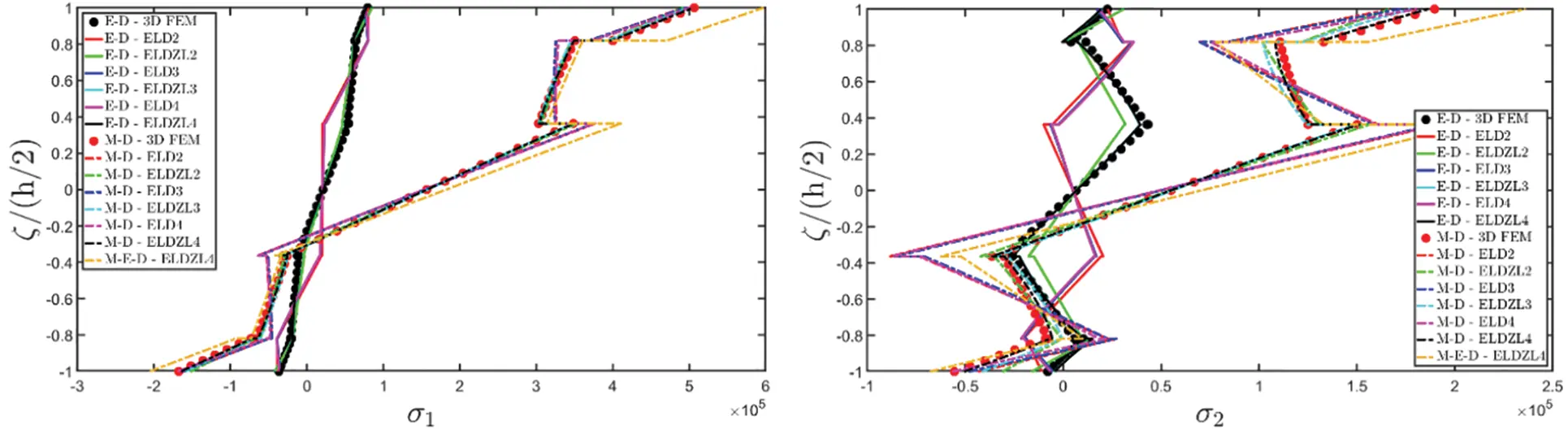

Figure 3: Through-the-thickness distributions of the components, expressed in (N/m2), of the 3D stress vector σ(α1,α2,ζ) of a simply-supported rectangular plate made of magneto-electro-elastic materials subjected to a sinusoidal distribution (N~=M~=1) of magnitude q¯D(+)=3.1×10⁻⁴C/m2 and q¯B(+)=−1.5×10⁻⁴Wb/m2 of an electric flux and a magnetic flux, respectively. Effect of fully coupling between electric and magnetic fields. The results are provided at (0.25L1,0.25L2) within the physical domain
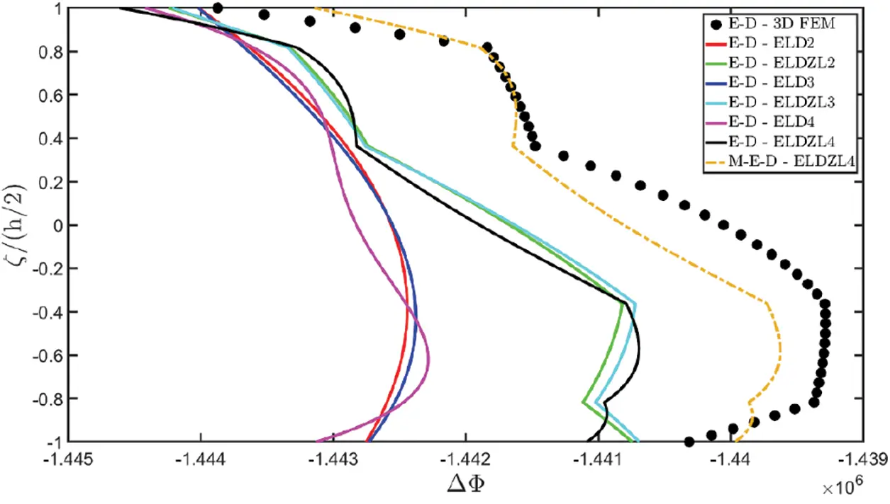

Figure 4: Through-the-thickness distributions of the variation of the electric potential ΔΦ(α1,α2,ζ) expressed in (V) and of the magnetic potential ΔΨ(α1,α2,ζ) expressed in (A) of a simply-supported rectangular plate made of magneto-electro-elastic materials subjected to a sinusoidal distribution (N~=M~=1) of magnitude q¯D(+)=3.1×10⁻⁴C/m2 and q¯B(+)=−1.5×10⁻⁴Wb/m2 of an electric flux and a magnetic flux, respectively. Effect of fully coupling between electric and magnetic fields. The results are provided at (0.25L1,0.25L2) within the physical domain
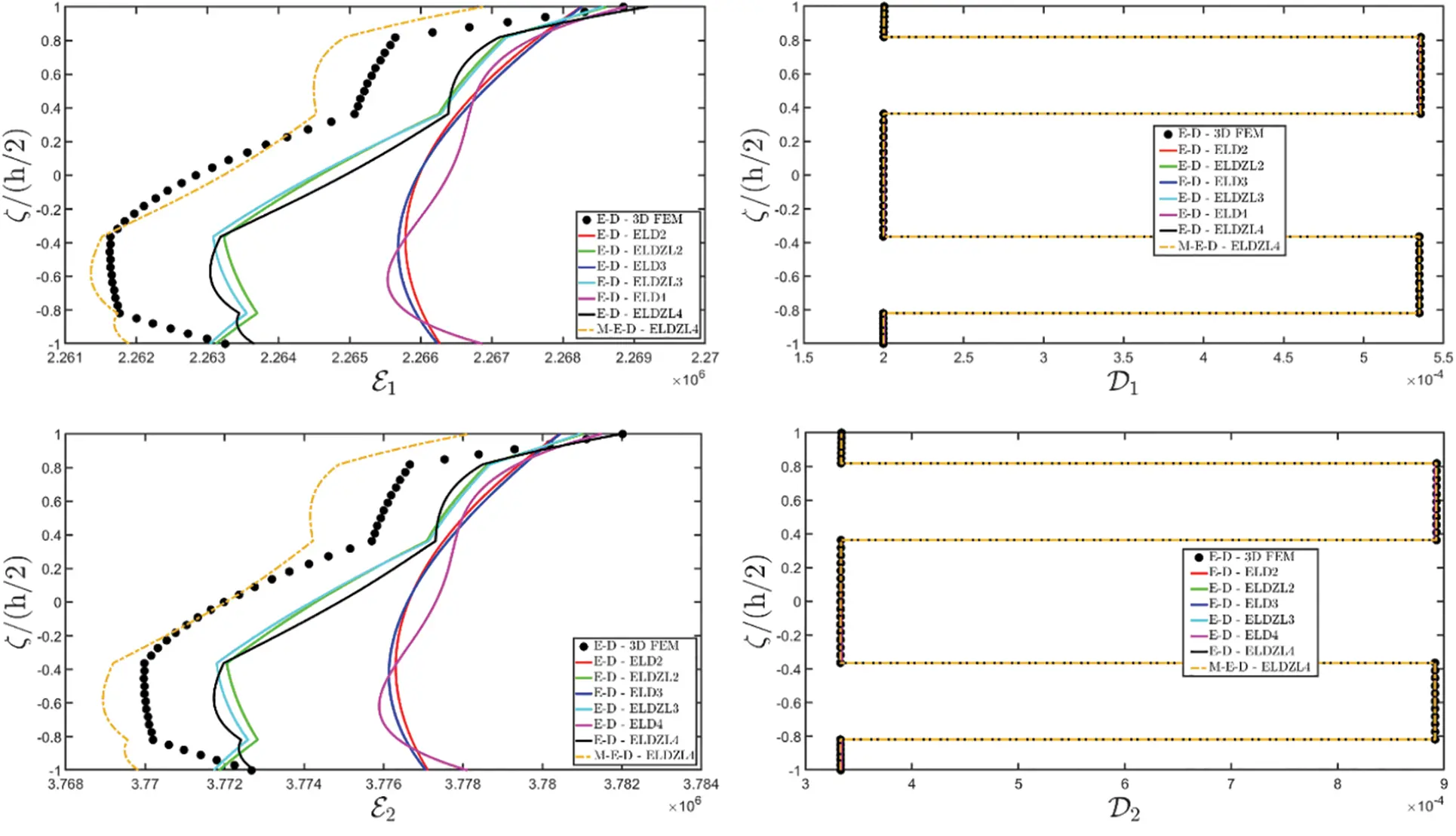

Figure 5: Through-the-thickness distributions of the components of the electric field vector E(α1,α2,ζ) (a) expressed in (V/m) and of the electric flux vector D(α1,α2,ζ) (b) expressed in (C/m2) of a simply-supported rectangular plate made of magneto-electro-elastic materials subjected to a sinusoidal distribution (N~=M~=1) of magnitude q¯D(+)=3.1×10⁻⁴C/m2 and q¯B(+)=−1.5×10⁻⁴Wb/m2 of an electric flux and a magnetic flux, respectively. Effect of fully coupling between electric and magnetic fields. The results are provided at (0.25L1,0.25L2) within the physical domain
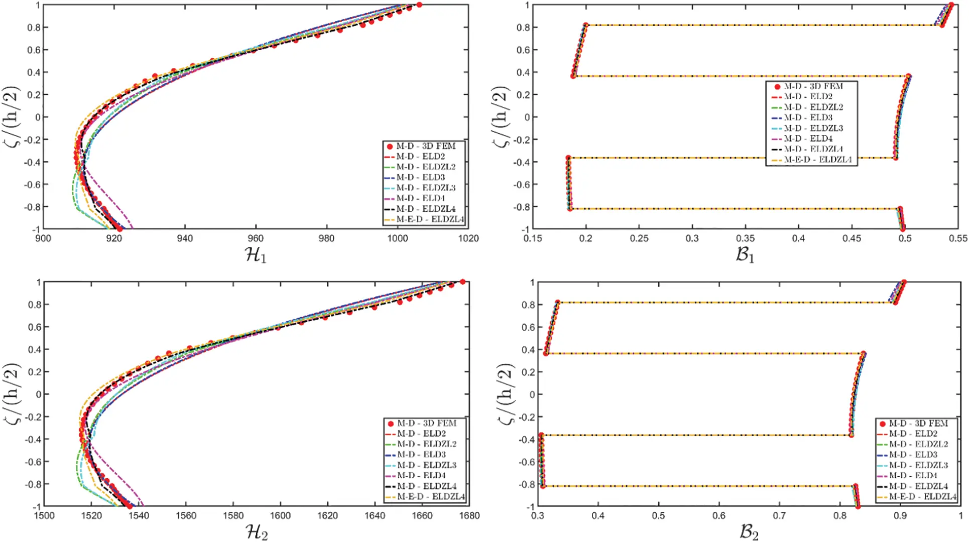

Figure 6: Through-the-thickness distributions of the components of the magnetic field vector H(α1,α2,ζ) (a) expressed in (A/m) and of the magnetic flux vector B(α1,α2,ζ) (b) expressed in (Wb/m2) of a simply-supported rectangular plate made of magneto-electro-elastic materials subjected to a sinusoidal distribution (N~=M~=1) of magnitude q¯D(+)=3.1×10⁻⁴C/m2 and q¯B(+)=−1.5×10⁻⁴Wb/m2 of an electric flux and a magnetic flux, respectively. Effect of fully coupling between electric and magnetic fields. The results are provided at (0.25L1,0.25L2) within the physical domain
The lamination scheme exhibits a characteristic zigzag behavior under both electric and magnetic fluxes. As a consequence, Murakami’s zigzag function is essential to align with 3D FEM numerical predictions. Furthermore, a higher-order kinematic model is required for deriving the bending response of the structure with a sufficient level of accuracy. This aspect may be physically interpreted as the fact that the panel while undergoing total deflection, exhibits a certain stretching within each lamina of the stacking sequence. Furthermore, the deformation of adjacent laminae is different, especially in the distortion components, while different slopes are found for the axial strain profiles. Furthermore, an abrupt slope change of displacement field is found, along with a stepwise variation in deformation components, especially for in-plane distortion components.
The presence of an external electric field induces a reduction in the vertical deflection of the plate due to the piezomagnetic response of the shell. Fig. 2 illustrates the 3D strain components for each simulation, where higher-order expansions of the unknown field variable, along with the ELW zigzag function, match accurately the 3D FEM-based numerical predictions. Conversely, lower-order theories like ELD3 and ELDZL3 exhibit inaccuracies. This aspect is particularly evident in Fig. 3, showing both in-plane and out-of-plane stress components against 3D FEM solutions. In particular, it is evident that the ELDZL4 is essential for deriving stable and accurate results. In addition, the GDQ-based numerical technique ensures the equilibrium under external loads at the top and bottom sides of the panel. The variation of the electric and magnetic potentials with respect to the undeformed configuration can be found in Fig. 4. Here, the stepwise volume fraction variation of piezoelectric and piezomagnetic materials along the thickness direction provides a typical zigzag behavior of the configuration variables. Near the top surface, E-D simulations demonstrate a higher accuracy due to a better alignment with finite element predictions. On the other hand, the zigzag effect is less evident for M-D simulations. This aspect can be physically interpreted remembering that the constitutive properties of adjacent laminae are similar, since they depend on the phase with higher volume fraction, with a negligible variation in the multifield response. In Fig. 5, some significant variations in the electric field and electric displacement components can be observed among adjacent laminae, showing the impact of electro-magnetic coupling on the fundamental equations and deviation from the profile of piezoelectric simulation. In the same way, perfect alignment is found in the out-of-plane components coming from the post-processing recovery procedure, which is valid, also, in multifield investigations. Similar considerations can be found in Fig. 6, where the magnetic displacement components are collected in columns (a) and (b), respectively. Unlike the previous case, in M-D simulations, the zigzag effect is prominent in the out-of-plane components, but less visible in others.
In the next example, the magneto-electric response of a laminated circular cylinder is investigated. The reference surface of the panel under consideration is defined as follows, with s1=R1α1 and s2=α2 representing the curvilinear lengths of the shell [48]:
r(s1,s2)=r(φ,y)=R1cosφe1−ye2+R1sinφe3(105)
As can be seen, the parametrization with curvilinear coordination is chosen such that the α2 axis aligns with the straight direction, while α1 direction exhibits a uniform curvature radius R1=0.8m. The physical domain is defined by [α10,α11]=[−π/2,2π/3] and [α20,α21]=[0,L2], with L2=2.1m. The material sequence (MEE−2/MEE−1/MEE−3/MEE−1/MEE−2) consists of five different laminae with thicknesses h1=h5=0.010m, h2=h4=0.025m and h3=0.040m. A null angle is assigned for the material reference system rotation in all layers of the stacking sequence. In contrast to the previous example, the central core, made of MEE-3, is characterized by a volume fraction of cylindrical fibers equal to Vf=0.15, while the value Vf=0.05 was selected for the central core of the rectangular plate of the previous case. Electric and magnetic loads are applied with a uniform distribution at the top and bottom surfaces of the cylinder. The magnitudes of magneto-electric fluxes are those of Eq. (104), as previously considered for the rectangular plate. The thickness plots of primary and secondary variables, evaluated at the point (0.75L1,0.25L2) setting N~=M~=35, are presented in Figs. 7–12.
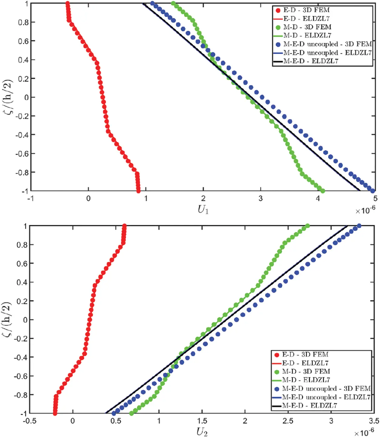

Figure 7: Through-the-thickness distributions of the components, expressed in (m), of the 3D displacement field vector U(α1,α2,ζ) of a simply-supported circular cylinder made of magneto-electro-elastic materials subjected to uniform distributions of magnitudes q¯D(+)=3.1×10⁻⁴C/m2, q¯D(−)=−1.5×10⁻⁴C/m2 and q¯B(+)=3.5×10⁻¹Wb/m2, q¯B(−)=−1.2×10⁻²Wb/m2 of an electric flux and a magnetic flux, respectively. Effect of fully coupling between electric and magnetic fields. The semi-analytical solution is derived for N~=M~=35. The results are provided at (0.75L1,0.25L2) within the physical domain
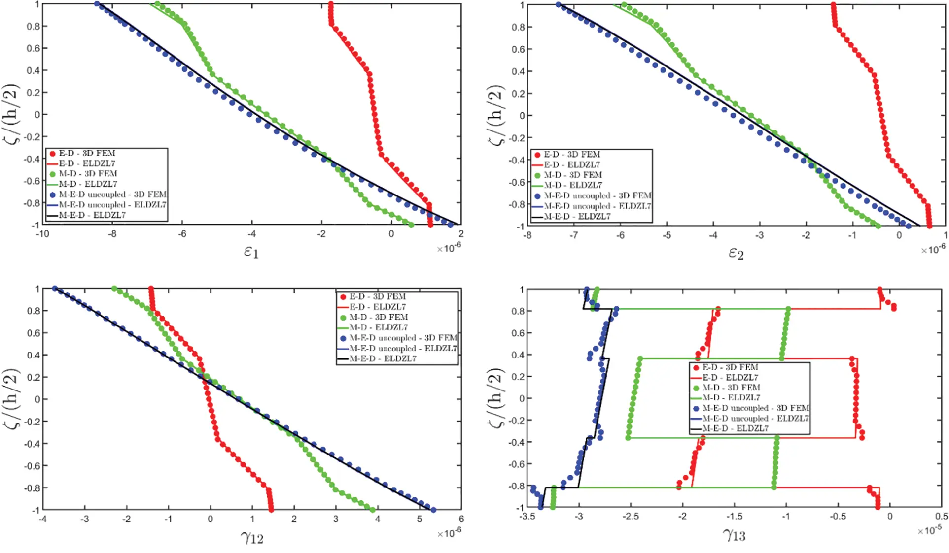

Figure 8: Through-the-thickness distributions of the components, expressed in(m/m), of the 3D strain vector ε(α1,α2,ζ) of a simply-supported circular cylinder made of magneto-electro-elastic materials subjected to uniform distributions of magnitudes q¯D(+)=3.1×10⁻⁴C/m2, q¯D(−)=−1.5×10⁻⁴C/m2 and q¯B(+)=3.5×10⁻¹Wb/m2, q¯B(−)=−1.2×10⁻²Wb/m2 of an electric flux and a magnetic flux, respectively. Effect of fully coupling between electric and magnetic fields. The semi-analytical solution is derived for N~=M~=35. The results are provided at (0.75L1,0.25L2) within the physical domain
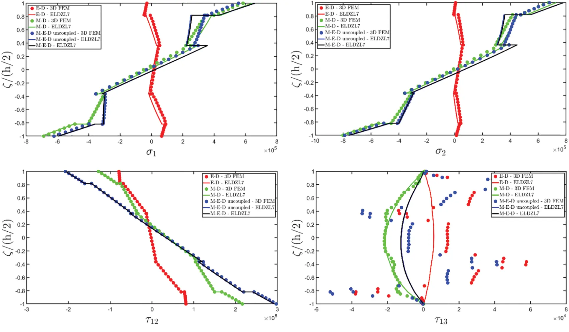

Figure 9: Through-the-thickness distributions of the components, expressed in (N/m2), of the 3D stress vector σ(α1,α2,ζ) of a simply-supported circular cylinder made of magneto-electro-elastic materials subjected to uniform distributions of magnitudes q¯D(+)=3.1×10⁻⁴C/m2, q¯D(−)=−1.5×10⁻⁴C/m2 and q¯B(+)=3.5×10⁻¹Wb/m2, q¯B(−)=−1.2×10⁻²Wb/m2 of an electric flux and a magnetic flux, respectively. Effect of fully coupling between electric and magnetic fields. The semi-analytical solution is derived for N~=M~=35. The results are provided at (0.75L1,0.25L2) within the physical domain

Figure 10: Through-the-thickness distributions of the variation of the electric potential ΔΦ(α1,α2,ζ) expressed in (V) and of the magnetic potential ΔΨ(α1,α2,ζ) expressed in (A) of a simply-supported circular cylinder made of magneto-electro-elastic materials subjected to uniform distributions of magnitudes q¯D(+)=3.1×10⁻⁴C/m2, q¯D(−)=−1.5×10⁻⁴C/m2 and q¯B(+)=3.5×10⁻¹Wb/m2, q¯B(−)=−1.2×10⁻²Wb/m2 of an electric flux and a magnetic flux, respectively. Effect of fully coupling between electric and magnetic fields. The semi-analytical solution is derived for N~=M~=35. The results are provided at (0.75L1,0.25L2) within the physical domain

Figure 11: Through-the-thickness distributions of the components of the electric field vector E(α1,α2,ζ) (a) expressed in (V/m) and of the electric flux vector D(α1,α2,ζ) (b) expressed in (C/m2) of a simply-supported circular cylinder made of magneto-electro-elastic materials subjected to uniform distributions of magnitudes q¯D(+)=3.1×10⁻⁴C/m2, q¯D(−)=−1.5×10⁻⁴C/m2 and q¯B(+)=3.5×10⁻¹Wb/m2, q¯B(−)=−1.2×10⁻²Wb/m2 of an electric flux and a magnetic flux, respectively. Effect of fully coupling between electric and magnetic fields. The semi-analytical solution is derived for N~=M~=35. The results are provided at (0.75L1,0.25L2) within the physical domain

Figure 12: Through-the-thickness distributions of the components of the magnetic field vector H(α1,α2,ζ) (a) expressed in (A/m) and of the magnetic flux vector B(α1,α2,ζ) (b) expressed in (Wb/m2) of a simply-supported circular cylinder made of magneto-electro-elastic materials subjected to uniform distributions of magnitudes q¯D(+)=3.1×10⁻⁴C/m2, q¯D(−)=−1.5×10⁻⁴C/m2 and q¯B(+)=3.5×10⁻¹Wb/m2, q¯B(−)=−1.2×10⁻²Wb/m2 of an electric flux and a magnetic flux, respectively. Effect of fully coupling between electric and magnetic fields. The semi-analytical solution is derived for N~=M~=35. The results are provided at (0.75L1,0.25L2) within the physical domain
The structural model is compared against 3D FEM reference solutions, considering the piezoelectric and magnetostatic response of the panel. In addition, an uncoupled M-E-D reference solution is provided, in which the piezoelectric and piezomagnetic effects are simultaneously evaluated without magneto-electric coupling. After some preliminary validation simulations, not included here for brevity, it is demonstrated that the ELDZL7 higher-order theory best matches numerical results with sufficient accuracy. Referring to the displacement field components of Fig. 7, a typical zigzag behavior is seen in both E-D and M-D numerical predictions, particularly evident for in-plane variables. This behavior is not observed in M-E-D simulations. Similar considerations apply to fully-coupled M-E-D results. In Fig. 8, the thickness plots of 3D strain components demonstrate an excellent agreement between the present results and those obtained from FEM, considering all possible coupling effects occurring at the interface between subsequent layers.
On the other hand, any meaningful differences can be observed between coupled and uncoupled M-E-D results. For 3D stress components (Fig. 9), it is evident that in-plane normal stresses from M-D and M-E-D simulations are higher compared to stress distributions obtained from E-D problems. In addition, despite the absence of an external mechanical load, out-of-plane normal and shear stresses are induced within the structure, with a peak in the middle core of the shell. The variation of electrostatic and magnetostatic potential is reported in Fig. 10. The distribution of the magnetostatic potential ΔΦ is not significantly characterized by a zigzag behavior, because the magnetic coefficients are less influenced by volume fraction variations of fibrous composites, mainly depending on the isotropic matrix. On the other hand, the electric potential exhibits an abrupt slope variation in its profile from one layer to another. From a physical point of view, it can be said that the 3D multifield response of the panel cannot be analyzed with classical lower-order theories as extensively done in the literature. These models, indeed, cannot be simultaneously suitable for predicting smooth and zigzag distributions of electric and magnetic potentials. In addition, the absence of the zigzag effect leads to a parabolic profile of multifield configuration variables, therefore a higher-order kinematic model is essential for deriving accurate and physically consistent results, in line with 3D simulations. Note that, for the selected lamination scheme, uncoupled M-E-D and fully coupled M-E-D simulations yield identical solutions. However, slight variations are observed among results in terms of electric field components, as reported in Fig. 11, when considering electromagnetic coupling in M-E-D numerical investigations. From a physical perspective, this means that the presence of a magnetic field slightly influences, in this case, the electric response of the laminate. Finally, the application of the post-processing recovery procedure ensures a perfect balance between external electric fluxes and internal out-of-plane electric displacement components at the top and bottom surfaces. A variation between uncoupled M-E-D and fully-coupled M-E-D results can be observed for the in-plane components of the magnetostatic field, depending on the presence of an external electric flux acting on the cylinder, as depicted in Fig. 12. Nevertheless, for both electric and magnetic primary and secondary variables, the model is successfully validated against numerical predictions obtained from FEM.
Previous investigation accounted for the evaluation of the mechanical response under electric and magnetic surface loads. In other words, the laminate has been studied for actuator configuration, since the application of multifield loads results in a variation of electric and magnetic potential within the laminate structure. As a consequence, a further numerical simulation is conducted where the present ELW formulation is employed to investigate the magneto-electro-elastic response of the same cylinder under a uniform distribution of the surface traction of magnitude q¯3(−)=−7.0×10⁴N/m2 applied at the top surface. In this case, the structure rests on a Winkler elastic foundation with elastic spring stiffness k3f(−)=5.0×10⁸N/m3. The results, evaluated at (0.75L1,0.25L2), can be found in Figs. 13–18. Even in this simulation, a reference solution is provided for E-D, M-D and uncoupled M-E-D cases. The semi-analytical solution is calculated with N~=M~=35 using the ELDZL7 kinematic model. Thickness plots for displacement field components, reported in Fig. 13, show that the cylinder, investigated in the previous example, does not exhibit any zigzag deformation under mechanical loads. However, the vertical deflection of the panel in terms of out-of-plane displacement component is not uniform along the thickness direction. As a consequence, a higher-order polynomial is essential to accurately predict the actual response of the shell. In this case, despite the structure being subjected to mechanical loads, the displacement field components of E-D and M-E-D simulations slightly deviate from M-D, because a part of the total energy of the system results in electric and magnetic fields, respectively. This aspect is less evident for the 3D strain components in Fig. 14, where only the out-of-plane axial strain exhibits a variation in the upper layers. On the other hand, the profiles of in-plane strain components are typical of classical lamination schemes with composite materials. On the other hand, the out-of-plane strain component ε3 exhibits a non-uniform distribution.

Figure 13: Through-the-thickness distributions of the components, expressed in (m), of the 3D displacement field vector U(α1,α2,ζ) of a simply supported circular cylinder made of magneto-electro-elastic materials subjected to uniformly distributed mechanical pressure of magnitude q¯3(+)=−7×10⁴N/m2 lying on an elastic foundation. Effect of fully coupling between electric and magnetic fields. The semi-analytical solution is derived for N~=M~=35. The results are provided at (0.75L1,0.25L2) within the physical domain

Figure 14: Through-the-thickness distributions of the components, expressed in (m/m), of the 3D strain vector ε(α1,α2,ζ) of a simply supported circular cylinder made of magneto-electro-elastic materials subjected to uniformly distributed mechanical pressure of magnitude q¯3(+)=−7×10⁴N/m2 lying on an elastic foundation. Effect of fully coupling between electric and magnetic fields. The semi-analytical solution is derived for N~=M~=35. The results are provided at (0.75L1,0.25L2) within the physical domain

Figure 15: Through-the-thickness distributions of the components, expressed in (N/m2), of the 3D stress vector σ(α1,α2,ζ) of a simply supported circular cylinder made of magneto-electro-elastic materials subjected to uniformly distributed mechanical pressure of magnitude q¯3(+)=−7×10⁴N/m2 lying on an elastic foundation. Effect of fully coupling between electric and magnetic fields. The semi-analytical solution is derived for N~=M~=35. The results are provided at (0.75L1,0.25L2) within the physical domain

Figure 16: Through-the-thickness distributions of the variation of the electric potential ΔΦ(α1,α2,ζ) expressed in (V) and of the magnetic potential ΔΨ(α1,α2,ζ) expressed in (A) of a simply supported circular cylinder made of magneto-electro-elastic materials subjected to uniformly distributed mechanical pressure of magnitude q¯3(+)=−7×10⁴N/m2 lying on an elastic foundation. Effect of fully coupling between electric and magnetic fields. The semi-analytical solution is derived for N~=M~=35. The results are provided at (0.75L1,0.25L2) within the physical domain
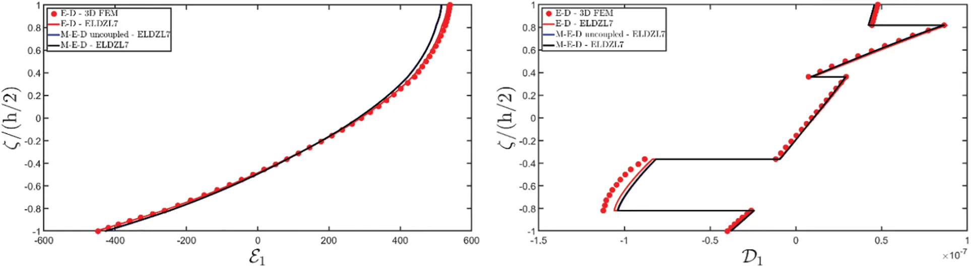

Figure 17: Through-the-thickness distributions of the components of the electric field vector E(α1,α2,ζ) (a) expressed in (V/m) and of the electric flux vector D(α1,α2,ζ) (b) expressed in (C/m2) of a simply supported circular cylinder made of magneto-electro-elastic materials subjected to uniformly distributed mechanical pressure of magnitude q¯3(+)=−7×10⁴N/m2 lying on an elastic foundation. Effect of fully coupling between electric and magnetic fields. The semi-analytical solution is derived for N~=M~=35. The results are provided at (0.75L1,0.25L2) within the physical domain


Figure 18: Through-the-thickness distributions of the components of the magnetic field vector H(α1,α2,ζ) (a) expressed in (A/m) and of the magnetic flux vector B(α1,α2,ζ) (b) expressed in (Wb/m2) of a simply supported circular cylinder made of magneto-electro-elastic materials subjected to uniformly distributed mechanical pressure of magnitude q¯3(+)=−7×10⁴N/m2 lying on an elastic foundation. Effect of fully coupling between electric and magnetic fields. The semi-analytical solution is derived for N~=M~=35. The results are provided at (0.75L1,0.25L2) within the physical domain
Therefore, a higher-order theory is essential to predict accurately the reference solution of the 3D numerical model. Fig. 15 displays the 3D stress components for the point under consideration, pointing out the excellent level of accuracy achieved by the semi-analytical model against finite element results. Furthermore, it is demonstrated that the coupling between electric and magnetic fields does not influence the structure when subjected to mechanical loads. Fig. 16 presents the through-the-thickness dispersion of electrostatic and magnetostatic potentials, derived through the 3D FEM model and the present higher-order formulation. As can be seen, the numerical model can predict the response of the structure for M-D, while the semi-analytical theory exhibits a variation in the magnetostatic potential in M-E-D simulation arising from the magneto-electric properties of the constituent materials. For the sake of completeness, the results for electric primary and secondary variables are shown in Fig. 17, while the magnetic field components and the magnetic flux components are represented in Fig. 18. It is observed that the electric response of the panel is slightly influenced by the presence of an external magnetic field, as evident among the semi-analytical results from E-D and M-E-D simulations. Similar considerations can be repeated for the magnetic field and flux components. In this last case, despite some discrepancies between the reference solution and the semi-analytical results, it should be noted that the balance of magnetic fluxes under external magnetic loads is perfectly satisfied at the top and bottom surfaces of the panel, due to the recovery procedure based on the adoption of the GDQ numerical method.
In the last example, we examine a simply supported doubly-curved spherical panel under various combinations of magneto-electro-elastic loads. The structure is characterized by the curvilinear lengths s1=R1α1=Rα1 and s2=R2α2=Rα2, with (α1,α2)∈[α10,α11]×[α20,α21]=[7π/18,11π/18]×[−π/3,π/3], according to the following relation [48]:
r(α1,α2)=R0(α1)cosα2e1−R0(α1)sinα2e2+(R−R2−(R0(α1))2)e3,R0(α1)=Rsinα1(106)
The principal curvature radius is equal to R1=R2=R=1.5m. The panel consists of five layers of thickness h1=h5=0.010m, h2=h4=0.025m and h3=0.040m, while the material sequence is (MEE−1/MEE−2/MEE−1/MEE−2/MEE−1), as defined in the previous examples. A concentrated mechanical load of magnitude q¯3(+)=−7.0×10⁴N is applied at the top surface at (s10,s20)=(0.75L1,0.75L2), within the physical domain. In addition, a mechanical patch load of magnitude q¯3(−)=3.0×10⁴N/m2 and shape parameters (c10,c20)=(0.25L1,0.25L2) is applied at the bottom surface of the shell, located at (s10,s20)=(0.75L1,0.75L2). In other words, a uniform surface traction is applied in a portion of the bottom surface, while the other parts remain unloaded. Regarding the magnetic and electric loads, two hydrostatic loads along α1 and α2, respectively, are applied at the top surface with q¯D(−)=3.1×10⁻⁴C/m2 and q¯B(+)=3.5×10⁻¹Wb/m2, while uniform distributions with magnitudes q¯D(−)=−1.5×10⁴C/m2 and q¯B(−)=−1.2×10⁻¹Wb/m2 are applied at the bottom surface. The multifield response of the shell is illustrated in Figs. 19–24, showing the thickness plots of the configuration variables, primary, and secondary variables at (0.75L1,0.25L2) within the physical domain. The semi-analytical solution is computed with N~=M~=50. As visible in Fig. 19, the shell undergoes a typical deflection with zigzag effects under multi field external actions due to the discrete variation of the volume fraction of the magneto-electro-elastic material constituents along the thickness directions in E-D and M-D simulations. However, when electric and magnetic fluxes are applied in M-E-D problems, the zigzag behavior is neglected, and the displacement field components show a linear through-the-thickness distribution. Furthermore, both uncoupled and coupled M-E-D solutions result in a slight variation of U3 vertical deflection. The magneto-electric coupling dependence of the structural response is less evident in the 3D strain components shown in Fig. 20. Unlike the displacement field components, M-E-D results exhibit a zigzag variation of in-plane strain components at the bottom side of the panel, while a smoother profile is observed at the top surface. The out-of-plane strain components γ13,γ23 and ε3 obtained from M-E-D simulations are similar to M-D results more than E-D simulations. This indicates that these strain components are predominantly induced, for the selected lamination scheme, by the external magnetic flux rather than the electric fluxes. Although the magneto-electric coupling influence is not prominent in the strain components, the 3D stress components depicted in Fig. 21 present a variation in the τ13 profile, when the magneto-electric coefficients are considered in the simulation. While in-plane stress components are significantly affected by magneto-electric external loads, the through-the-thickness profile of out-of-plane normal stress mainly depends on the mechanical pressures applied at the top surface.

Figure 19: Through-the-thickness distributions of the components, expressed in (m), of the 3D displacement field vector U(α1,α2,ζ) of a simply-supported spherical panel made of magneto-electro-elastic materials subjected to a combination of concentrated, uniform, hydrostatic, and patch multifield load shapes. The results are obtained from a semi-analytical Navier solution with N~=M~=50. Effect of fully coupling between electric and magnetic fields. The results are provided at (0.75L1,0.25L2) within the physical domain

Figure 20: Through-the-thickness distributions of the components, expressed in (m/m), of the 3D strain vector ε(α1,α2,ζ) of a simply-supported spherical panel made of magneto-electro-elastic materials subjected to a combination of concentrated, uniform, hydrostatic, and patch multifield load shapes. The results are obtained from a semi-analytical Navier solution with N~=M~=50. Effect of fully coupling between electric and magnetic fields. The results are provided at (0.75L1,0.25L2) within the physical domain

Figure 21: Through-the-thickness distributions of the components, expressed in (N/m2), of the 3D stress vector σ(α1,α2,ζ) of a simply-supported spherical panel made of magneto-electro-elastic materials subjected to a combination of concentrated, uniform, hydrostatic, and patch multifield load shapes. The results are obtained from a semi-analytical Navier solution with N~=M~=50. Effect of fully coupling between electric and magnetic fields. The results are provided at (0.75L1,0.25L2) within the physical domain

Figure 22: Through-the-thickness distributions of the variation of the electric potential ΔΦ(α1,α2,ζ) expressed in (V) and of the magnetic potential ΔΨ(α1,α2,ζ) expressed in (A) of a simply-supported spherical panel made of magneto-electro-elastic materials subjected to a combination of concentrated, uniform, hydrostatic, and patch multifield load shapes. The results are obtained from a semi-analytical Navier solution with N~=M~=50. Effect of fully coupling between electric and magnetic fields. The results are provided at (0.75L1,0.25L2) within the physical domain
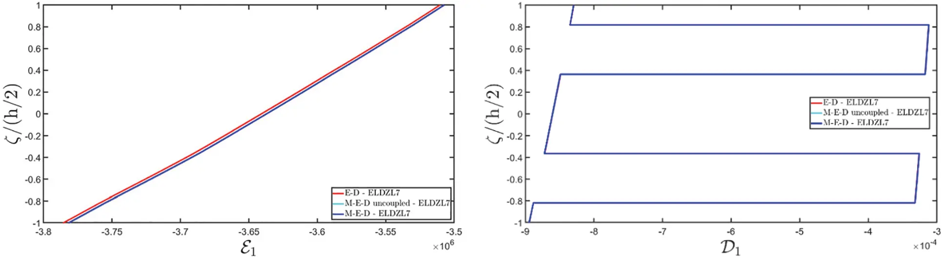

Figure 23: Through-the-thickness distributions of the components of the electric field vector E(α1,α2,ζ) (a) expressed in (V/m) and of the electric flux vector D(α1,α2,ζ) (b) expressed in (C/m2) of a simply-supported spherical panel made of magneto-electro-elastic materials subjected to a combination of concentrated, uniform, hydrostatic, and patch multifield load shapes. The results are obtained from a semi-analytical Navier solution with N~=M~=50. Effect of fully coupling between electric and magnetic fields. The results are provided at (0.75L1,0.25L2) within the physical domain
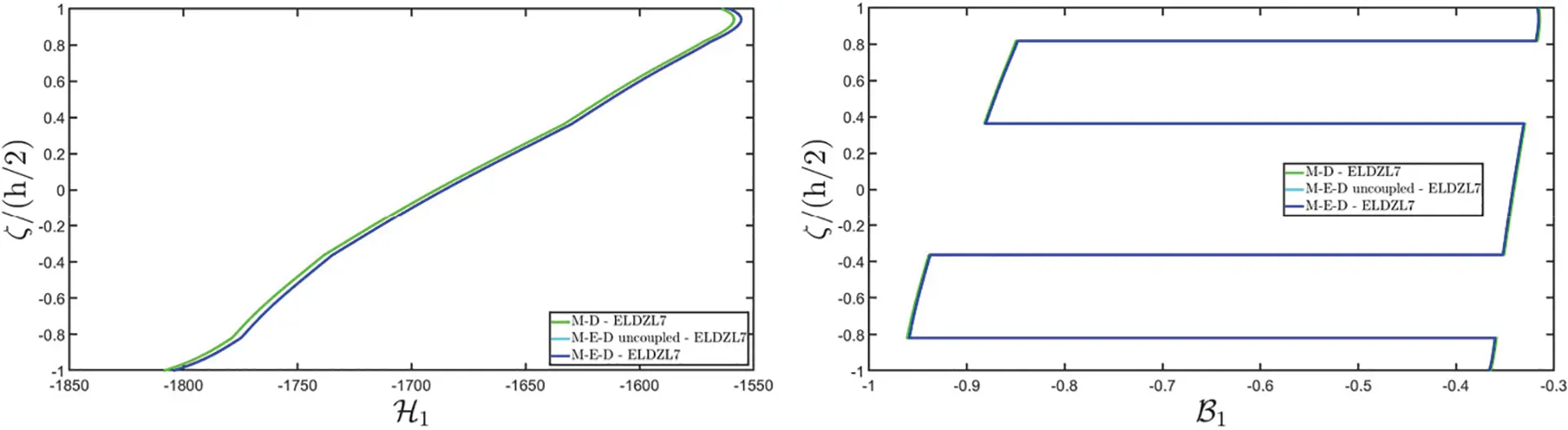

Figure 24: Through-the-thickness distributions of the components of the magnetic field vector H(α1,α2,ζ) (a) expressed in (A/m) and of the magnetic flux vector B(α1,α2,ζ) (b) expressed in (Wb/m2) of a simply-supported spherical panel made of magneto-electro-elastic materials subjected to a combination of concentrated, uniform, hydrostatic, and patch multifield load shapes. The results are obtained from a semi-analytical Navier solution with N~=M~=50. Effect of fully coupling between electric and magnetic fields. The results are provided at (0.75L1,0.25L2) within the physical domain
The simultaneous application of electric and magnetic external actions to the panel results in a shift of the electric and magnetic potential profiles, as shown in Fig. 22. For all loading conditions, a slope variation of these scalar quantities occurs at each interface between two subsequent laminae. Furthermore, the highest variation in the magnetic potential is found in those layers exhibiting a uniform distribution of electric potential, while a significant variation in the electric potential occurs when a uniform dispersion of magnetic potential is present.
As finally shown in Figs. 23 and 24, the thickness plots of the electric and magnetic primary and secondary variables feature a smooth variation for in-plane components, while ℰ3 and ℋ3 significantly vary between two adjacent layers. The out-of-plane components of electric and magnetic fluxes, instead, exhibit a continuous variation in their profile, despite the presence of a zigzag behavior. On the other hand, in-plane components are described by stepwise functions.
From all the numerical examples presented in this study, some important conclusions can be derived. In particular, the results demonstrate that, in general, the actual response of moderately thick laminated panels under mechanical, magnetic, and electric loads, has a 3D behavior. As a consequence, the classical kinematic model should not be adopted to derive a proper description of the structural response, especially when out-of-plane variables are required. On the other hand, the through-the-thickness kinematic assumption should consider higher-order basis functions, along with zigzag functions to predict the stretching and the squeezing of each lamina, along with the zigzag behavior at the interface. Another important aspect is that the required order of the thickness function should be higher for electric and magnetic potential than that adopted in the mechanical elasticity case. As a consequence, a possible enhancement of the theory should consider different kinematic assumptions for each unknown variable in the model. Referring to the constitutive properties, the magneto-electric coupling can induce additional values of electric and magnetic fields. For this reason, it is essential to consider the coupling terms within the formulation, otherwise, the numerical predictions may be inaccurate, especially for electric and magnetic primary and secondary variables. Finally, the adoption of a Navier-type solution, even though based on specific assumptions on materials, geometry, and boundary conditions, can be adopted for various multifield loading conditions by properly expanding the solution due to the convergence of Fourier trigonometric series. On the other hand, for prescribed values of multifield configuration variables at the top and bottom surfaces, only sinusoidal distributions can be adopted, because the boundary conditions with null values of electric and magnetic potentials must be satisfied at the four edges of the 2D parametric domain.
10 Conclusions
A novel higher-order theory has been proposed in this work for the magneto-electro-elastic analysis of laminated shell structures with varying curvatures. This theory employs a generalized method to model the distribution of the displacement field components, electrostatic, and magnetostatic potential, accounting for higher-order polynomials. The thickness functions have been defined to prescribe the arbitrary values of configuration variables at the top and bottom surfaces, even though the model is ESL-based. The fundamental governing equations have been derived in curvilinear principal coordinates, considering all coupling effects among different physical phenomena, including piezoelectric, piezomagnetic, and magneto-electric effects. A homogenization algorithm based on a Mori & Tanaka approach has been adopted to obtain the equivalent magneto-electro-mechanical properties of a two-phase transversely isotropic composite. In addition, an effective method has been adopted involving the external loads in terms of surface tractions, as well as the electric and magnetic fluxes. In the post-processing stage, a GDQ-based procedure provides the actual 3D response of a doubly-curved solid. The model has been validated through significant numerical examples, showing that the results of this semi-analytical theory align well with those obtained from 3D numerical models from commercial codes. In particular, the accuracy of the model has been verified for lamination schemes with soft layers and various curvatures under different loading conditions. Moreover, this formulation has been used to predict the effect of combined electric and magnetic loads on the mechanical response of panels with different curvatures and lamination schemes. As a consequence, this theory can be applied in engineering applications where the combined effect of electric and magnetic loads is crucial, thus facilitating their study and design. An existing limitation of this study is that the solution is that it is derived only for structures with uniform curvature, cross-ply lamination scheme, and simply supported boundary conditions. Furthermore, it requires that each lamina within the stacking sequence exhibits magneto-electro-elastic behavior. Therefore, at the present stage, it cannot be used for multifield analysis of classical composite structures with magneto-electric patches. A further enhancement of the research work could be the derivation of a solution employing a numerical technique, to overcome the limitations of the Navier method. In this way, the same theory may be adopted to predict the multifield response of structures with variable curvatures and thickness, as well as anisotropic materials and more complicated boundary conditions.
Acknowledgement: The authors are grateful to the Department of Innovation Engineering of University of Salento for the support.
Funding Statement: The paper has been funded by the Project PNRR M4C2—Innovation Grant DIRECT: Digital twIns foR EmergenCy supporT—CUP F83C22000740001.
Author Contributions: Francesco Tornabene: Writing—review & editing, Visualization, Validation, Supervision, Software, Methodology, Investigation, Formal analysis, Data curation, Conceptualization. Matteo Viscoti: Writing—original draft, Validation, Investigation, Data curation. Rossana Dimitri: Writing—review & editing, Validation, Supervision, Investigation, Formal analysis, Conceptualization. All authors reviewed the results and approved the final version of the manuscript.
Availability of Data and Materials: Data and materials are available upon request.
Ethics Approval: Not applicable.
Conflicts of Interest: The authors declare no conflicts of interest to report regarding the present study.
References
1. Kapuria S, Kumari P, Nath JK. Efficient modeling of smart piezoelectric composite laminates: a review. Acta Mech. 2010;214(1):31–48. doi:10.1007/s00707-010-0310-0. [Google Scholar] [CrossRef]
2. Mahapatra SD, Mohapatra PC, Aria AI, Christie G, Mishra YK, Hofmann S, et al. Piezoelectric materials for energy harvesting and sensing applications: roadmap for future smart materials. Adv Sci. 2021;8(17):2100864. doi:10.1002/advs.202100864. [Google Scholar] [PubMed] [CrossRef]
3. Tichý J, Erhart J, Kittinger E, Privratska J. Fundamentals of piezoelectric sensorics: mechanical, dielectric, and thermodynamical properties of piezoelectric materials. Heidelberg: Springer Science & Business Media; 2010. [Google Scholar]
4. Basheer AA. Advances in the smart materials applications in the aerospace industries. Aircr Eng Aerosp Technol. 2020;92(7):1027–35. doi:10.1108/AEAT-02-2020-0040. [Google Scholar] [CrossRef]
5. Narita F, Fox M. A review on piezoelectric, magnetostrictive, and magnetoelectric materials and device technologies for energy harvesting applications. Adv Eng Mater. 2018;20(5):1700743. doi:10.1002/adem.201700743. [Google Scholar] [CrossRef]
6. Sezer N, Koç M. A comprehensive review on the state-of-the-art of piezoelectric energy harvesting. Nano Energy. 2021;80(1):105567. doi:10.1016/j.nanoen.2020.105567. [Google Scholar] [CrossRef]
7. Han JH, Lee I. Analysis of composite plates with piezoelectric actuators for vibration control using layerwise displacement theory. Compos B Eng. 1998;29(5):621–32. doi:10.1016/S1359-8368(98)00027-4. [Google Scholar] [CrossRef]
8. Ikeda T. Fundamentals of piezoelectricity. Oxford: Oxford University Press; 1996. [Google Scholar]
9. Tiersten HF. Thickness vibrations of piezoelectric plate. J Acoust Soc Am. 1963;35(1):53–8. doi:10.1121/1.1918413. [Google Scholar] [CrossRef]
10. Li X, Lu SG, Chen XZ, Gu H, Quian XS, Zhang QM. Pyroelectric and electrocaloric materials. J Mater Chem C. 2013;1:23–37. doi:10.1039/C2TC00283C. [Google Scholar] [CrossRef]
11. Zhang D, Wu H, Bowen CR, Yang Y. Recent advances in pyroelectric materials and applications. Small. 2021;17(51):2103960. doi:10.1002/smll.202103960. [Google Scholar] [PubMed] [CrossRef]
12. Benveniste Y. Magnetoelectric effect in fibrous composites with piezoelectric and piezomagnetic phases. Phys Rev B. 1995;51(22):16424. doi:10.1103/PhysRevB.51.16424. [Google Scholar] [PubMed] [CrossRef]
13. Avellaneda M, Harshé G. Magnetoelectric effect in piezoelectric/magnetostrictive multilayer (2-2) composites. J Intell Mater Syst Struct. 1994;5(4):501–13. [Google Scholar]
14. Ortega N, Kumar A, Scott JF, Katiyar RS. Multifunctional magnetoelectric materials for device applications. J Phys Condens Matter. 2015;27(50):504002. [Google Scholar] [PubMed]
15. Bracke LPM, Van Vliet RG. A broadband magneto-electric transducer using a composite material. Int J Electron. 1981;51(3):255–62. [Google Scholar]
16. Nan CW, Bichurin MI, Dong S, Viehland D, Srinivasan G. Multiferroic magnetoelectric composites: historical perspective, status, and future directions. J Appl Phys. 2008;103(3):31101. [Google Scholar]
17. Van Suchtelen J. Product properties: a new application of composite materials. Philips Res Rep. 1972;27(1):28–37. [Google Scholar]
18. Newnham RE, Skinner DP, Cross LE. Connectivity and piezoelectric-pyroelectric composites. Mater Res Bull. 1978;13(5):525–36. doi:10.1016/0025-5408(78)90161-7. [Google Scholar] [CrossRef]
19. Van den Boomgaard J, Born RAJ. A sintered magnetoelectric composite material BaTiO3Ni(Co, Mn) Fe2O4. J Mater Sci. 1978;13(1):1538–48. doi:10.1007/BF00553210. [Google Scholar] [CrossRef]
20. Dong S, Zhai J, Bai F, Li JF, Viehland D. Push-pull mode magnetostrictive/piezoelectric laminate composite with an enhanced magnetoelectric voltage coefficient. Appl Phys Lett. 2005;87(6):62502. doi:10.1063/1.2007868. [Google Scholar] [CrossRef]
21. Srinivasan G, Tatarenko AS, Bichurin MI. Electrically tunable microwave filters based on ferromagnetic resonance in ferrite-ferroelectric bilayers. Electron Lett. 2005;41(10):596–8. doi:10.1049/el:20050925. [Google Scholar] [CrossRef]
22. Osaretin IA, Rojas RG. Theoretical model for the magnetoelectric effect in magnetostrictive/piezoelectric composites. Phys Rev B. 2010;82(17):174415. doi:10.1103/PhysRevB.82.174415. [Google Scholar] [CrossRef]
23. Monge JC, Mantari JL. Thermal bending response of functionally graded magneto-electric-elastic shell employing non-polynomial model. Mech Adv Mater Struct. 2023;30(14):2882–98. doi:10.1080/15376494.2022.2064570. [Google Scholar] [CrossRef]
24. Ryu J, Carazo AV, Uchino K, Kim HE. Magnetoelectric properties in piezoelectric and magnetostrictive laminate composites. Jpn J Appl Phys. 2001;40(8R):4948. doi:10.1143/JJAP.40.4948. [Google Scholar] [CrossRef]
25. Bichurin M, Petrov V. Modeling of magnetoelectric effects in composites. Dordrecht: Springer; 2014. [Google Scholar]
26. Dunn ML, Taya M. An analysis of piezoelectric composite materials containing ellipsoidal inhomogeneities. Proc R Soc Lond Ser A. 1993;443(1918):265–87. doi:10.1098/rspa.1993.0145. [Google Scholar] [CrossRef]
27. Harshe G, Dougherty JP, Newnham RE. Theoretical modelling of multilayer magnetoelectric composites. Int J Appl Electromagn Mech. 1993;4(2):145–5. [Google Scholar]
28. Wang TZ, Zhou YH. A theoretical study of nonlinear magnetoelectric effect in magnetostrictive-piezoelectric trilayer. Compos Struct. 2011;93(5):1485–92. [Google Scholar]
29. Li JY, Dunn ML. Micromechanics of magnetoelectroelastic composite materials: average fields and effective behavior. J Intell Mater Syst Struct. 1998;9(6):404–16. doi:10.1177/1045389X9800900602. [Google Scholar] [CrossRef]
30. Mori T, Tanaka K. Average stress in matrix and average elastic energy of materials with misfitting inclusions. Acta Metall. 1973;21(5):571–4. doi:10.1016/0001-6160(73)90064-3. [Google Scholar] [CrossRef]
31. Pan E, Han F. Exact solution for functionally graded and layered magneto-electro-elastic plates. Int J Eng Sci. 2005;43(3–4):321–39. doi:10.1016/j.ijengsci.2004.09.006. [Google Scholar] [CrossRef]
32. Akbarzadeh A, Chen Z. Thermo-magneto-electro-elastic responses of rotating hollow cylinders. Mech Adv Mater Struct. 2014;21(1):67–80. doi:10.1080/15376494.2012.677108. [Google Scholar] [CrossRef]
33. Yue Y, Ye X, Xu K. Analytical solutions for plane problem of functionally graded magnetoelectric cantilever beam. Appl Math Mech. 2015;36(7):955–70. doi:10.1007/s10483-015-1980-9. [Google Scholar] [CrossRef]
34. Liu J, Foo CC, Zhang ZQ. A 3D multi-field element for simulating the electromechanical coupling behavior of dielectric elastomers. Acta Mech Solida Sin. 2017;30(4):374–89. doi:10.1016/j.camss.2017.07.005. [Google Scholar] [CrossRef]
35. Tounsi A, Tahir SI, Al-Osta MA, Do-Van T, Bourada F, Bousahla AA, et al. An integral quasi-3D computational model for the hygro-thermal wave propagation of imperfect FGM sandwich plates. Comput Concr. 2023;32(1):61–74. [Google Scholar]
36. Monge JC, Mantari JL. Three-dimensional numerical solution for the bending study of magneto-piezo-elastic spherical and cylindrical shells. Eng Struct. 2021;238(1):112158. doi:10.1016/j.engstruct.2021.112158. [Google Scholar] [CrossRef]
37. Sih GC, Michopoulos JG, Chou SC. Hygrothermoelasticity. Dordrecht: Martinus Nijhoff Publishers; 1986. [Google Scholar]
38. Landau LD, Lifshitz EM. The classical theory of fields. Oxford: Pergamon Press; 1951. [Google Scholar]
39. Zhou L, Li M, Cai Y, Zhao H, Zhao E. The multi-physic cell-based smoothed finite element method for dynamic characterization of magneto-electro-elastic structures under thermal conditions. Compos Struct. 2020;240(1):112045. doi:10.1016/j.compstruct.2020.112045. [Google Scholar] [CrossRef]
40. Zhou L, Yang H, Ma L, Zhang S, Li X, Ren S, et al. On the static analysis of inhomogeneous magneto-electro-elastic plates in thermal environment via element-free Galerkin method. Eng Anal Bound Elem. 2022;134(1):539–52. doi:10.1016/j.enganabound.2021.11.002. [Google Scholar] [CrossRef]
41. Tornabene F, Viscoti M, Dimitri R. Equivalent layer-wise theory for the hygro-thermo-magneto-electro-elastic analysis of laminated curved shells. Thin-Walled Struct. 2024;198(1):111751. [Google Scholar]
42. Tornabene F, Viscoti M, Dimitri R. Thermo-mechanical analysis of laminated doubly-curved shells: higher order equivalent layer-wise formulation. Compos Struct. 2024;335(1):117995. [Google Scholar]
43. Tornabene F, Viscoti M, Dimitri R, Reddy JN. Higher order theories for the vibration study of doubly-curved anisotropic shells with a variable thickness and isogeometric mapped geometry. Compos Struct. 2021;267(1):113829. [Google Scholar]
44. Reddy JN. Mechanics of laminated composite plates and shells: theory and analysis. Boca Raton: CRC Press; 2003. [Google Scholar]
45. Reddy JN. An evaluation of equivalent-single-layer and layerwise theories of composite laminates. Compos Struct. 1993;25(1–4):21–35. [Google Scholar]
46. Reddy JN, Robbins DHJr. Theories and computational models for composite laminates. Appl Mech Rev. 1994;47(6):147–69. [Google Scholar]
47. Tornabene F, Fantuzzi N, Bacciocchi M, Reddy JN. An equivalent layer-wise approach for the free vibration analysis of thick and thin laminated and sandwich shells. Appl Sci. 2016;7(1):17. [Google Scholar]
48. Tornabene F. Hygro-thermo-magneto-electro-elastic theory of anisotropic doubly-curved shells. Bologna: Esculapio; 2023. [Google Scholar]
49. Tornabene F, Viscoti M, Dimitri R. Equivalent single layer higher order theory based on a weak formulation for the dynamic analysis of anisotropic doubly-curved shells with arbitrary geometry and variable thickness. Thin-Walled Struct. 2022;174(1):109119. [Google Scholar]
50. Liew KM, Pan ZZ, Zhang LW. An overview of layerwise theories for composite laminates and structures: development, numerical implementation and application. Compos Struct. 2019;216(1):240–59. [Google Scholar]
51. Monge JC, Mantari JL, Hinostroza MA. Non-polynomial hybrid models for the bending of magneto-electro-elastic shells. Mech Adv Mater Struct. 2024;31(17):4081–115. [Google Scholar]
52. Santapuri S, Scheidler JJ, Dapino MJ. Two-dimensional dynamic model for composite laminates with embedded magnetostrictive materials. Compos Struct. 2015;132(1):737–45. [Google Scholar]
53. Lim CW, Lau CWH. A new two-dimensional model for electro-mechanical response of thick laminated piezoelectric actuator. Int J Solids Struct. 2005;42(20):5589–611. doi:10.1016/j.ijsolstr.2005.02.050. [Google Scholar] [CrossRef]
54. Brischetto S, Torre R. Thermo-elastic analysis of multilayered plates and shells based on 1D and 3D heat conduction problems. Compos Struct. 2018;206(1):326–53. doi:10.1016/j.compstruct.2018.08.042. [Google Scholar] [CrossRef]
55. Brischetto S, Torre R. 3D shell model for the thermo-mechanical analysis of FGM structures via imposed and calculated temperature profiles. Aerosp Sci Technol. 2019;85(1):125–49. doi:10.1016/j.ast.2018.12.011. [Google Scholar] [CrossRef]
56. Washizu K. Variational methods in elasticity & plasticity. Oxford: Pergamon Press; 1975. [Google Scholar]
57. Reddy JN. A generalization of two-dimensional theories of laminated composite plates. Commun Appl Numer Methods. 1987;3(3):173–80. doi:10.1002/cnm.1630030303. [Google Scholar] [CrossRef]
58. Tornabene F, Viscoti M, Dimitri R. Static analysis of doubly-curved shell structures of smart materials and arbitrary shape subjected to general loads employing higher order theories and generalized differential quadrature method. Comput Model Eng Sci. 2022;133(3):22210. doi:10.32604/cmes.2022.022210. [Google Scholar] [CrossRef]
59. Wang CM, Reddy JN, Lee KH. Shear deformable beams and plates: relationships with classical solutions. Boca Raton: Elsevier; 2003. [Google Scholar]
60. Icardi U, Sola F. Assessment of recent zig-zag theories for laminated and sandwich structures. Compos B Eng. 2016;97(1):26–52. [Google Scholar]
61. Murakami H. Laminated composite plate theory with improved in-plane responses. J Appl Mech. 1986;53(3):661–6. [Google Scholar]
62. Tessler A, Di Sciuva M, Gherlone M. A refined zigzag beam theory for composite and sandwich beams. J Compos Mater. 2009;43(9):1051–81. [Google Scholar]
63. Gherlone M, Tessler A, Di Sciuva M. C0 beam elements based on the refined zigzag theory for multilayered composite and sandwich laminates. Compos Struct. 2011;93(11):2882–94. [Google Scholar]
64. Di Sciuva M, Sorrenti M. Bending and free vibration analysis of functionally graded sandwich plates: an assessment of the refined zigzag theory. J Sandw Struct Mater. 2021;23(3):760–802. [Google Scholar]
65. Al-Osta MA. An exponential-trigonometric quasi-3D HSDT for wave propagation in an exponentially graded plate with microstructural defects. Compos Struct. 2022;297(1):115984. doi:10.1016/j.compstruct.2022.115984. [Google Scholar] [CrossRef]
66. Wang J, Yang J. Higher-order theories of piezoelectric plates and applications. Appl Mech Rev. 2000;53(4):87–99. doi:10.1115/1.3097341. [Google Scholar] [CrossRef]
67. Aminipour H, Janghorban M, Civalek O. Analysis of functionally graded doubly-curved shells with different materials via higher order shear deformation theory. Compos Struct. 2020;251(1):112645. doi:10.1016/j.compstruct.2020.112645. [Google Scholar] [CrossRef]
68. Tornabene F, Viscoti M, Dimitri R. Higher order theories for the modal analysis of anisotropic doubly-curved shells with a three-dimensional variation of the material properties. Eng Anal Bound Elem. 2024;158(1):486–519. doi:10.1016/j.enganabound.2023.11.008. [Google Scholar] [CrossRef]
69. Batra RC, Vidoli S. Higher-order piezoelectric plate theory derived from a three-dimensional variational principle. AIAA J. 2002;40(1):91–104. doi:10.2514/2.1618. [Google Scholar] [CrossRef]
70. Wang J, Yong YK, Imai T. Finite element analysis of the piezoelectric vibrations of quartz plate resonators with higher-order plate theory. Int J Solids Struct. 1999;36(15):2303–19. doi:10.1016/S0020-7683(98)00108-5. [Google Scholar] [CrossRef]
71. Mantari JL, Oktem AS, Soares CG. Bending response of functionally graded plates by using a new higher order shear deformation theory. Compos Struct. 2012;94(2):714–23. doi:10.1016/j.compstruct.2011.09.007. [Google Scholar] [CrossRef]
72. Tu LW. Differential geometry: connections, curvature, and characteristic classes. Cham: Springer; 2017. [Google Scholar]
73. Gu DX, Saucan E. Classical and discrete differential geometry: theory, applications and algorithms. Boca Raton: CRC Press; 2023. [Google Scholar]
74. Oprea J. Differential geometry and its applications. London: Pearson; 2007. [Google Scholar]
75. Holzapfel GA. Nonlinear solid mechanics: a continuum approach for engineering science. Chichester: John Wiley & Sons; 2002. [Google Scholar]
76. Tornabene F, Viscoti M, Dimitri R. Static analysis of anisotropic doubly-curved shell subjected to concentrated loads employing higher order layer-wise theories. Comput Model Eng Sci. 2022;134(2):1393–468. doi:10.32604/cmes.2022.022237. [Google Scholar] [CrossRef]
77. Tornabene F, Viscoti M, Dimitri R. Free vibration analysis of laminated doubly-curved shells with arbitrary material orientation distribution employing higher order theories and differential quadrature method. Eng Anal Bound Elem. 2023;152(1):397–445. doi:10.1016/j.enganabound.2023.04.008. [Google Scholar] [CrossRef]
78. Laureano RW, Mantari JL, Yarasca J, Oktem AS, Monge J, Zhou X. Exact solutions for clamped spherical and cylindrical panels via a unified formulation and boundary discontinuous method. Compos Struct. 2024;346(1):118429. doi:10.1016/j.compstruct.2024.118429. [Google Scholar] [CrossRef]
79. Monge JC, Mantari JL. 3D elasticity numerical solution for the static behavior of FGM shells. Eng Struct. 2020;208:110159. doi:10.1016/j.engstruct.2019.110159. [Google Scholar] [CrossRef]
80. Chattopadhyay A, Li J, Gu H. Coupled thermo-piezoelectric-mechanical model for smart composite laminates. AIAA J. 1999;37(12):1633–8. doi:10.2514/2.645. [Google Scholar] [CrossRef]
81. Mitchell JA, Reddy JN. A refined hybrid plate theory for composite laminates with piezoelectric laminae. Int J Solids Struct. 1995;32(16):2345–67. doi:10.1016/0020-7683(94)00229-P. [Google Scholar] [CrossRef]
82. Bhangale RK, Ganesan N. Static analysis of simply supported functionally graded and layered magneto-electro-elastic plates. Int J Solids Struct. 2006;43(10):3230–53. doi:10.1016/j.ijsolstr.2005.05.030. [Google Scholar] [CrossRef]
83. Brischetto S. An exact 3D solution for free vibrations of multilayered cross-ply composite and sandwich plates and shells. Int J Appl Mech. 2014;6(6):1450076. doi:10.1142/S1758825114500768. [Google Scholar] [CrossRef]
84. Pagano NJ. Exact solutions for composite laminates in cylindrical bending. J Compos Mater. 1969;3(3):398–411. [Google Scholar]
85. Pagano NJ. Exact solutions for rectangular bidirectional composites and sandwich plates. J Compos Mater. 1970;4(1):20–34. [Google Scholar]
86. Tornabene F, Viscoti M, Dimitri R. On the importance of the recovery procedure in the semi-analytical solution for the static analysis of curved laminated panels: comparison with 3D finite elements. Materials. 2024;17(3):588. [Google Scholar] [PubMed]
87. Patton A, Antolin P, Dufour JE, Kiendl J, Reali A. Accurate equilibrium-based interlaminar stress recovery for isogeometric laminated composite Kirchhoff plates. Compos Struct. 2021;256(1):112976. [Google Scholar]
88. Reddy JN. Introduction to the finite element method. New York: McGraw-Hill Education; 2019. [Google Scholar]
89. Zienkiewicz OC, Taylor RL. The finite element method: solid mechanics. New York: McGraw-Hill; 1967. vol. 2. [Google Scholar]
90. Wu CP, Liu YC. A review of semi-analytical numerical methods for laminated composite and multilayered functionally graded elastic/piezoelectric plates and shells. Compos Struct. 2016;147(1):1–15. [Google Scholar]
91. Xiang Y, Wang Z, Zhang S, Jiang L, Lin Y, Tan J. Cross-sectional performance prediction of metal tubes bending with tangential variable boosting based on parameters-weight-adaptive CNN. Expert Syst Appl. 2024;237A(1):121465. doi:10.1016/j.eswa.2023.121465. [Google Scholar] [CrossRef]
92. Bert CW, Malik M. Differential quadrature method in computational mechanics: a review. Appl Mech Rev. 1996;49(1):1–28. doi:10.1115/1.3101882. [Google Scholar] [CrossRef]
93. Shu C. Differential quadrature and its application in engineering. Heidelberg: Springer Science & Business Media; 2012. [Google Scholar]
94. Tornabene F. Generalized differential and integral quadrature. Bologna: Esculapio; 2023. [Google Scholar]
95. Shu C, Chen W, Xue H, Du H. Numerical study of grid distribution effect on accuracy of DQ analysis of beams and plates by error estimation of derivative approximation. Int J Numer Methods Eng. 2001;51(2):159–79. doi:10.1002/nme.150. [Google Scholar] [CrossRef]
96. Shu C, Chen W. On optimal selection of interior points for applying discretized boundary conditions in DQ vibration analysis of beams and plates. J Sound Vib. 1999;222(2):239–57. doi:10.1006/jsvi.1998.2041. [Google Scholar] [CrossRef]
97. Tornabene F, Viscoti M, Dimitri R, Aiello MA. Higher order formulations for doubly-curved shell structures with a honeycomb core. Thin-Walled Struct. 2021;164(1):107789. doi:10.1016/j.tws.2021.107789. [Google Scholar] [CrossRef]
98. Fu T, Hu X, Yang C. Impact response analysis of stiffened sandwich functionally graded porous materials doubly-curved shell with re-entrant honeycomb auxetic core. Appl Math Model. 2023;124(1):553–75. doi:10.1016/j.apm.2023.08.024. [Google Scholar] [CrossRef]
99. Ghandehari MA, Masoodi AR, Panda SK. Thermal frequency analysis of double CNT-reinforced polymeric straight beam. J Vib Eng Technol. 2024;12(1):649–65. doi:10.1007/s42417-023-00865-0. [Google Scholar] [CrossRef]
100. Striz AG, Wang X, Bert CW. Harmonic differential quadrature method and applications to analysis of structural components. Acta Mech. 1995;111(1):85–94. doi:10.1007/BF01187729. [Google Scholar] [CrossRef]
101. Civalek Ö. Application of differential quadrature (DQ) and harmonic differential quadrature (HDQ) for buckling analysis of thin isotropic plates and elastic columns. Eng Struct. 2004;26(2):171–86. doi:10.1016/j.engstruct.2003.09.005. [Google Scholar] [CrossRef]
102. Chen W, Wang X, Zhong T. The structure of weighting coefficient matrices of harmonic differential quadrature and its applications. Commun Numer Methods Eng. 1996;12(8):455–9. [Google Scholar]
103. Shu C, Chew YT, Richards BE. Generalized differential and integral quadrature and their application to solve boundary layer equations. Int J Numer Methods Fluids. 1995;21(9):723–33. doi:10.1002/fld.1650210903. [Google Scholar] [CrossRef]
Appendix A
In this appendix we present some analytical expressions, derived from Reference [29], to determine the multifield constitutive relationship for a magneto-electro-elastic composite material with a fully linear static coupling between magnetic, electric and mechanical elasticity physical properties. The procedure is based on the Mori-Tanaka approach, as described in Reference [30], for a two-phase composite material consisting of an isotropic matrix (m) with continuous cylindrical fibers (f) aligned along the thickness direction, with volume fractions Vm and Vf, respectively. As a result, the homogenized material exhibits a transversely isotropic symmetry, being α1,α2 the isotropic plane. Note that the coupling between the electric and magnetic fields occurs only in the homogenized material, while the individual phases do not exhibit this property.
In what follows, the magneto-electro-mechanical properties of the matrix and fiber are expressed in the material reference system according to Eq. (35), with subscripts referring to the phases of the heterogeneous material.
Preliminary computations
j=2VfC44ml11mm11m+p14m2m11m+l11mq14m2−2d11mp14m−d11m2C44m(ic−gb)h+(fb−ia)e+(ga−fc)d
a=Vm((q14f−q14m)(l11mm11m−d11m2)−(d11f−d11m)(p14mm11m−d11mq14m)−(m11f−m11m)(q14ml11m−d11mp14m))
b=Vm((p14f−p14m)(l11mm11m−d11m2)−(d11f−d11m)(q14ml11m−d11mp14m)−(l11f−l11m)(p14mm11m−d11mq14m))
c=Vm((C44f−C44m)(l11mm11m−d11m2)+(p14f−p14m)(p14mm11m−d11mq14m)+(q14f−q14m)(q14ml11m−d11mp14m))+jVf((ic−gb)h+(fb−ia)e+(ga−fc)d)
d=Vm(−(d11f−d11m)(d11mC44m+p14mq14m)+(p14f−p14m)(p14mm11m−d11mq14m)+(l11f−l11m)(q14m2+C44mm11m))+jVf((ic−gb)h+(fb−ia)e+(ga−fc)d)
e=Vm((q14f−q14m)(d11mC44m+p14mq14m)+(C44f−C44m)(p14mm11m−d11mq14m)−(p14f−p14m)(q14m2+C44mm11m))
f=Vm(−(d11f−d11m)(d11mC44m+p14mq14m)+(q14f−q14m)(q14ml11m−d11mp14m)+(m11f−m11m)(p14m2+C44ml11m))+jVf((ic−gb)h+(fb−ia)e+(ga−fc)d)
g=Vm((p14f−p14m)(d11mC44m+p14mq14m)+(C44f−C44m)(q14ml11m−d11mp14m)−(q14f−q14m)(p14m2+C44ml11m))
h=Vm(−(m11f−m11m)(d11mC44m−p14mq14m)+(q14f−q14m)(p14mm11m−d11mq14m)+(d11f−d11m)(q14m2+C44mm11m))
i=Vm(−(l11f−l11m)(d11mC44m+p14mq14m)+(p14f−p14m)(q14ml11m−d11mp14m)+(d11f−d11m)(p14m2+C44ml11m))(A1)
Density
ρ=Vmρm+Vfρf(A2)
Elastic stiffness constants
k=kmkf+Vfmmkf+VmmmkmVmkf+Vfkm+mm
m=mm(kmmf+Vfkmmf+Vmkmmm+2mmmf)Vmkmmf+kmmm+Vfkmmm+2Vmmmmf+2Vfmm2
C11=C22=k+m
C12=k−m
C13=C23=C13m+Vf(C13f−C13m)(km+mm)Vmkf+Vfkm+mm
C33=C33m+Vf(C33f−C33m−Vm(C13m−C13f)2Vmkf+Vfkm+mm)
C44=C55=C44m+j((p14f−p14m)(fe−gh)+(C44f−C44m)(ih−fd)+(q14f−q14m)(gd−ie))(A3)
Piezoelectric constants
p31=p32=p31m+Vf(p31f−p31m)(km+mm)Vmkf+Vfkm+mm
p33=p33m+Vf(p33f−p33m+Vm(C13m−C13f)(p31f−p31m)Vmkf+Vfkm+mm)
p14=p25=p14m+j((p14f−p14m)(ga−fc)+(C44f−C44m)(fb−ia)+(q14f−q14m)(ic−gb))(A4)
Piezomagnetic or magneto-strictive constants
q31=q32=q31m+Vf(q31f−q31m)(km+mm)Vmkf+Vfkm+mm
q33=q33m+Vf(q33f−q33m+Vm(C13m−C13f)(q31f−q31m)Vmkf+Vfkm+mm)
q14=q25=q14m+j((p14f−p14m)(ch−ae)+(C44f−C44m)(ad−bh)+(q14f−q14m)(be−cd))(A5)
Dielectric permittivity constants
l11=l22=l11m+j((l11f−l11m)(ga−fc)+(p14f−p14m)(ia−fb)+(d11f−d11m)(ic−gb))
l33=l33m+Vf(l33f−l33m+Vm(p31f−p31m)2Vmkf+Vfkm+mm)(A6)
Magnetic permeability constants
m11=m22=m11m+j((d11f−d11m)(ch−ae)+(q14f−q14m)(bh−ad)+(m11f−m11m)(be−cd))
m33=m33m+Vf(m33f−m33m+Vm(m31f−m31m)2Vmkf+Vfkm+mm)(A7)
Magneto-electric constants
d11=d22=d11m+j((l11f−l11m)(ch−ae)+(p14f−p14m)(bh−ad)+(d11f−d11m)(be−cd))
d33=d33m+Vf(d33f−d33m−Vm(p31f−p31m)(q31m−q31f)Vmkf+Vfkm+mm)(A8)
Appendix B
In this appendix, the interested reader can find the complete expressions for the semi-analytical coefficients L~ijnm(τη)αiαj of the higher order ELW magneto-electro-elastic fundamental matrix L~nm(τη), as introduced in Eq. (73). The following expressions are valid for each n=1,…,N~ and m=1,…,M~. These expressions refer to the case of a doubly-curved shell panel with a uniform distribution of Lamé parameters and the values of the principal radii of curvature, according to Eq. (6).
L~11nm(τη)α1α1=−A11(20)(τη)[00]α1α1(nπL1)2−A66(02)(τη)[00]α1α1(mπL2)2−A44(20)(τη)[00]α1α1R12+A44(10)(τη)[01]α1α1+A44(10)(τη)[10]α1α1R1−A44(00)(τη)[11]α1α1
L~12nm(τη)α1α2=−(A12(11)(τη)[00]α1α2+A66(11)(τη)[00]α1α2)(nπL1)(mπL2)
L~13nm(τη)α1α3=(A13(10)(τη)[01]α1α3−A44(10)(τη)[10]α1α3+A11(20)(τη)[00]α1α3+A44(20)(τη)[00]α1α3R1+A12(11)(τη)[00]α1α3R2)(nπL1)
L~14nm(τη)α1α4=(P31(10)(τη)[01]α1α4−P14(10)(τη)[10]α1α4+P14(20)(τη)[00]α1α4R1)(nπL1)
L~15nm(τη)α1α5=(Q31(10)(τη)[01]α1α5−Q14(10)(τη)[10]α1α5+Q14(20)(τη)[00]α1α5R1)(nπL1)
L~21nm(τη)α2α1=−(A12(11)(τη)[00]α2α1+A66(11)(τη)[00]α2α1)(nπL1)(mπL2)
L~22nm(τη)α2α2=−A66(20)(τη)[00]α2α2(nπL1)2−A22(02)(τη)[00]α2α2(mπL2)2−A55(02)(τη)[00]α2α2R22+A55(01)(τη)[01]α2α2+A55(01)(τη)[10]α2α2R2−A55(00)(τη)[11]α2α2
L~23nm(τη)α2α3=(A23(01)(τη)[01]α2α3−A55(01)(τη)[10]α2α3+A22(02)(τη)[00]α2α3+A55(02)(τη)[00]α2α3R2+A12(11)(τη)[00]α2α3R1)(mπL2)
L~24nm(τη)α2α4=(P32(01)(τη)[01]α2α4−P25(01)(τη)[10]α2α4+P25(02)(τη)[00]α2α4R2)(mπL2)
L~25nm(τη)α2α5=(Q32(01)(τη)[01]α2α5−Q25(01)(τη)[10]α2α5+Q25(02)(τη)[00]α2α5R2)(mπL2)
L~31nm(τη)α3α1=(A13(10)(τη)[10]α3α1−A44(10)(τη)[01]α3α1+A11(20)(τη)[00]α3α1+A44(20)(τη)[00]α3α1R1+A12(11)(τη)[00]α3α1R2)(nπL1)
L~32nm(τη)α3α2=(A23(01)(τη)[10]α3α2−A55(01)(τη)[01]α3α2+A12(11)(τη)[00]α3α2R1+A22(02)(τη)[00]α3α2+A55(02)(τη)[00]α3α2R2)(mπL2)
L~33nm(τη)α3α3=−A44(20)(τη)[00]α3α3(nπL1)2−A55(02)(τη)[00]α3α3(mπL2)2−A11(20)(τη)[00]α3α3R12−A22(02)(τη)[00]α3α3R22−2A12(11)(τη)[00]α3α3R1R2+
−A13(10)(τη)[01]α3α3+A13(10)(τη)[10]α3α3R1−A23(01)(τη)[01]α3α3+A23(01)(τη)[10]α3α3R2−A33(00)(τη)[11]α3α3
L~34nm(τs)α3α4=−P14(20)(τη)[00]α3α4(nπL1)2−P25(02)(τη)[00]α3α4(mπL2)2−P31(10)(τη)[01]α3α4R1−P32(01)(τη)[01]α3α4R2−P33(00)(τη)[11]α3α4
L~35nm(τη)α3α5=−Q14(20)(τη)[00]α3α5(nπL1)2−Q25(02)(τη)[00]α3α5(mπL2)2−Q31(10)(τη)[01]α3α5R1−Q32(01)(τη)[01]α3α5R2−Q33(00)(τη)[11]α3α5
L~41nm(τη)α4α1=−(P14(10)(τη)[01]α4α1−P31(10)(τη)[10]α4α1−P14(20)(τη)[00]α4α1R1)(nπL1)
L~42nm(τη)α4α2=−(P25(01)(τη)[01]α4α2−P32(01)(τη)[10]α4α2−P25(02)(τη)[00]α4α2R2)(mπL2)
L~43nm(τη)α4α3=−P14(20)(τη)[00]α4α3(nπL1)2−P25(02)(τη)[00]α4α3(mπL2)2−P31(10)(τη)[10]α4α3R1−P32(01)(τη)[10]α4α3R2−P33(00)(τη)[11]α4α3
L~44nm(τη)α4α4=L11(20)(τη)[00]α4α4(nπL1)2+L22(02)(τη)[00]α4α4(mπL2)2+L33(00)(τη)[11]α4α4
L~45nm(τη)α4α5=D11(20)(τη)[00]α4α5(nπL1)2+D22(02)(τη)[00]α4α5(mπL2)2+D33(00)(τη)[11]α4α5
L~51nm(τη)α5α1=−(Q14(10)(τη)[01]α5α1−Q31(10)(τη)[10]α5α1−Q14(20)(τη)[00]α5α1R1)(nπL1)
L~52nm(τη)α5α2=−(Q25(01)(τη)[01]α5α2−Q32(01)(τη)[10]α5α2−Q25(02)(τη)[00]α5α2R2)(mπL2)
L~53nm(τη)α5α3=−Q14(20)(τη)[00]α5α3(nπL1)2−Q25(02)(τη)[00]α5α3(mπL2)2−Q31(10)(τη)[10]α5α3R1−Q32(01)(τη)[10]α5α3R2−Q33(00)(τη)[11]α5α3
L~54nm(τη)α5α4=D11(20)(τη)[00]α5α4(nπL1)2+D22(02)(τη)[00]α5α4(mπL2)2+D33(00)(τη)[11]α5α4
L~55nm(τη)α5α5=M11(20)(τη)[00]α5α5(nπL1)2+M22(02)(τη)[00]α5α5(mπL2)2+M33(00)(τη)[11]α5α5(A9)
The expressions provided above can be simplified for the case of a cylindrical panel with straight directrix along α1,α2, considering that in the first case it is 1/R1=0. On the other hand, when the directrix is oriented along α2, the semi-analytical fundamental coefficients are derived from the previous relations by setting 1/R2=0. Similarly, the fundamental coefficients for a rectangular plate of size L1 and L2 along α1,α2, respectively, can be written by setting 1/R1=0 and 1/R2=0.

 Submit a Paper
 Propose a Special lssue
 Open Access
 View Full Text
 Download PDF
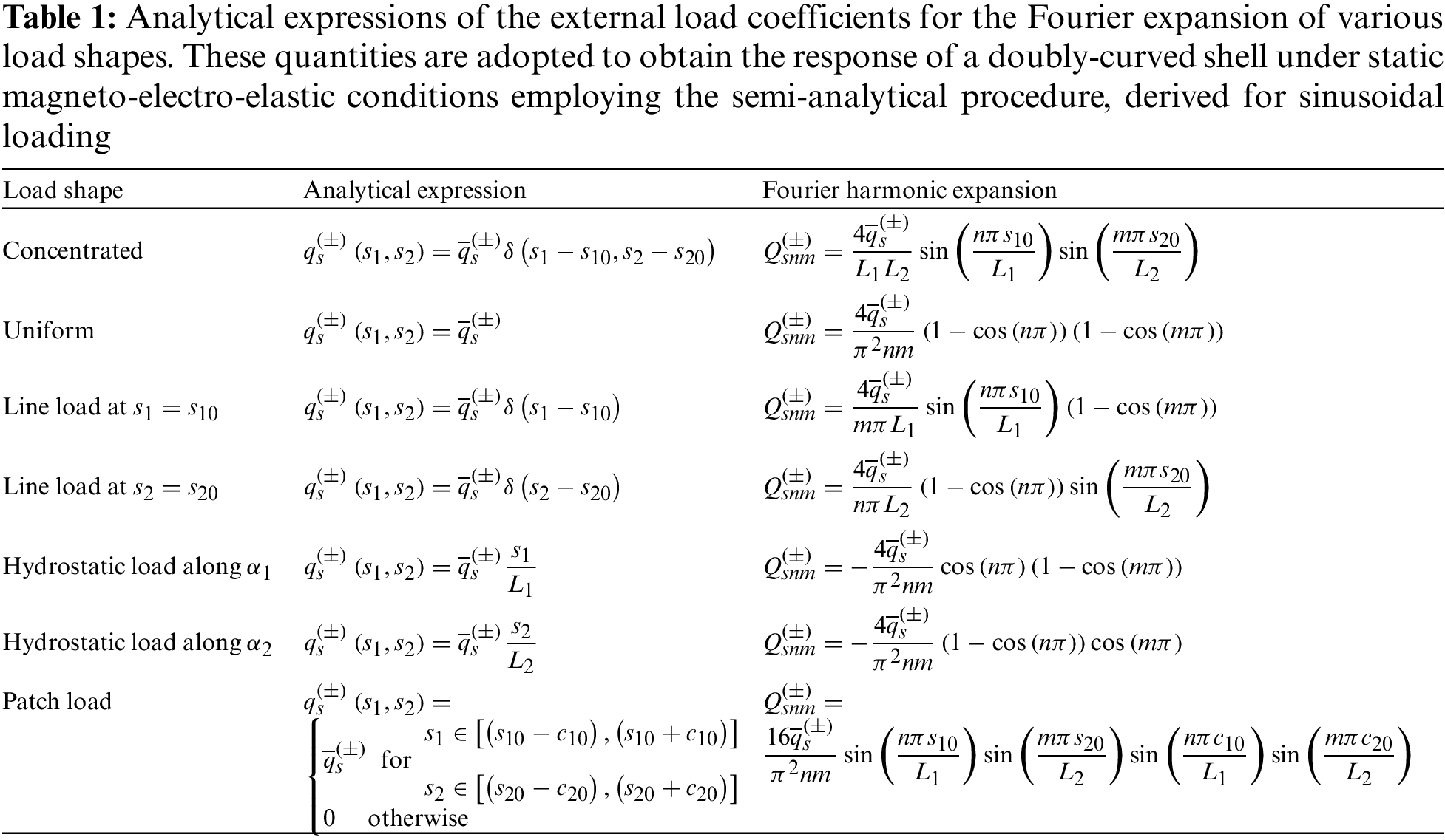


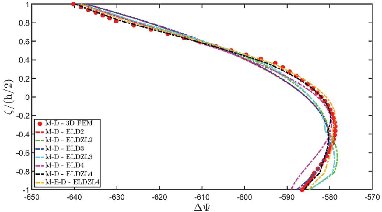
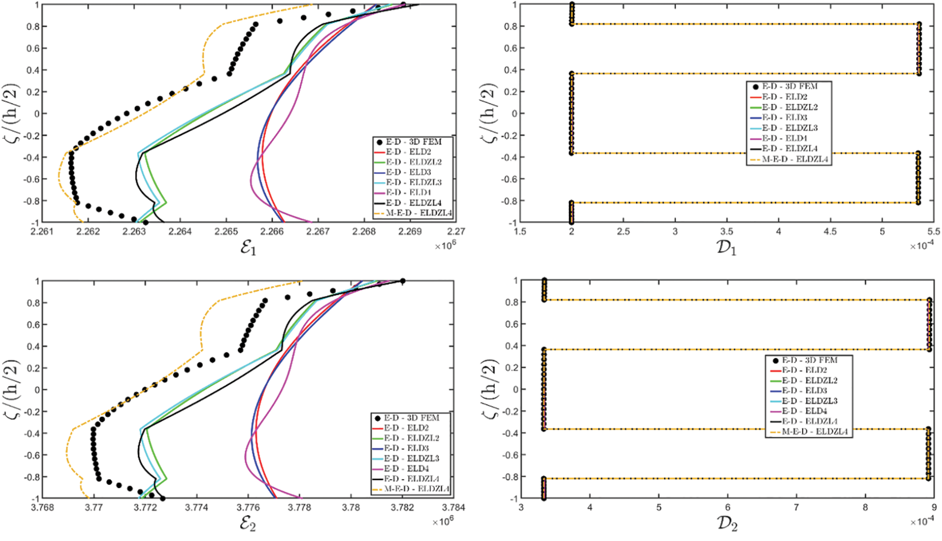
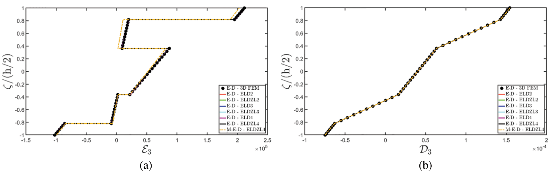


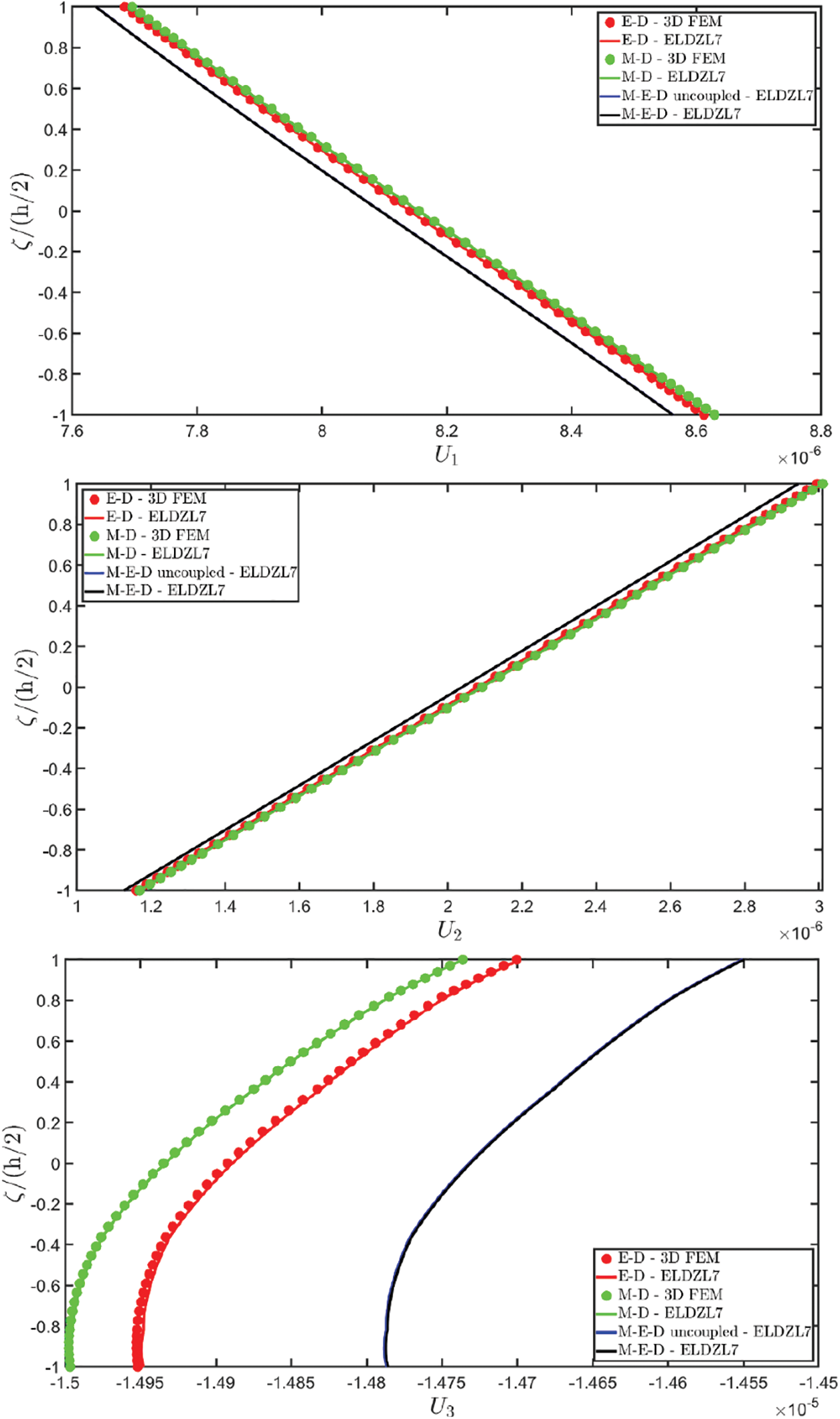
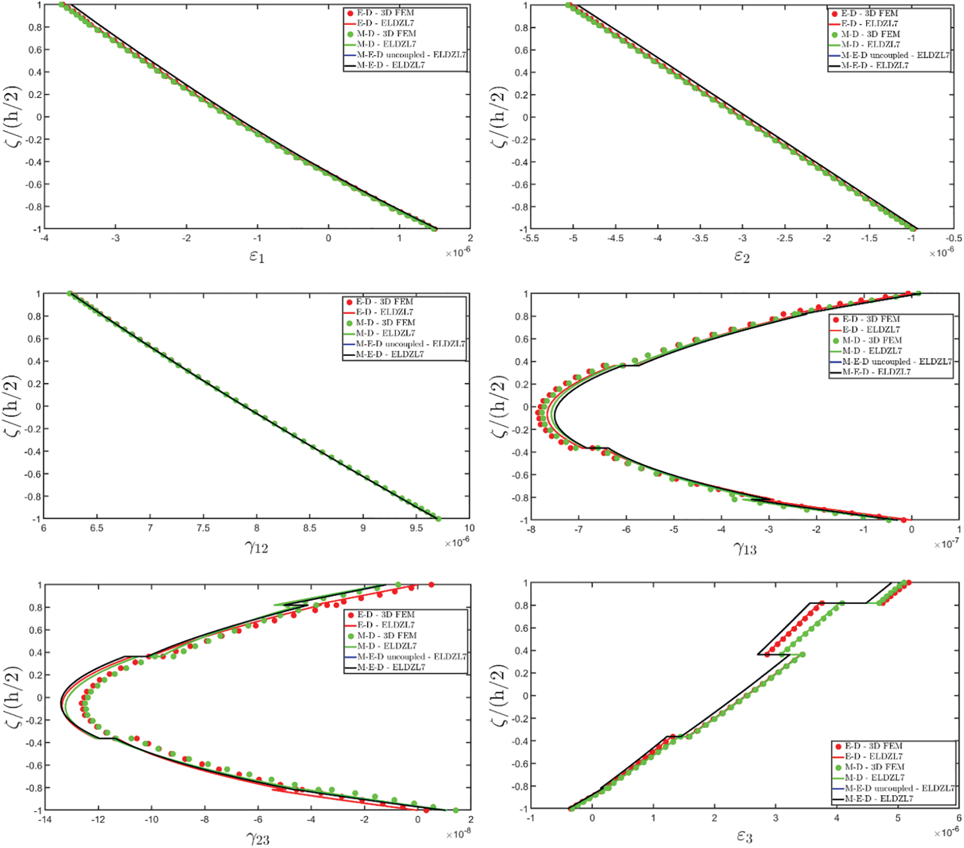
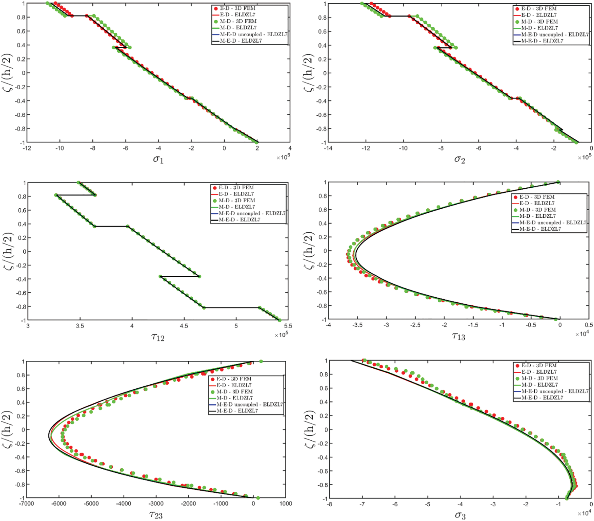


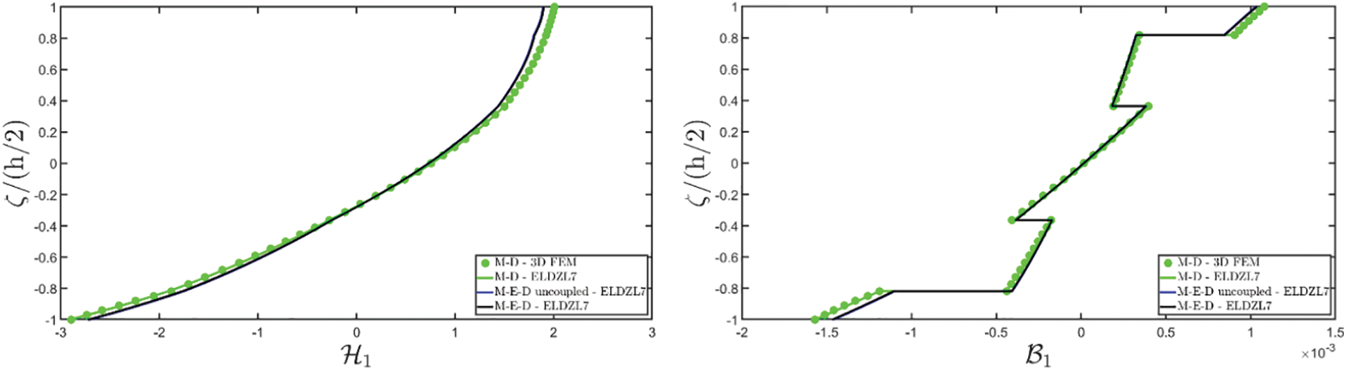

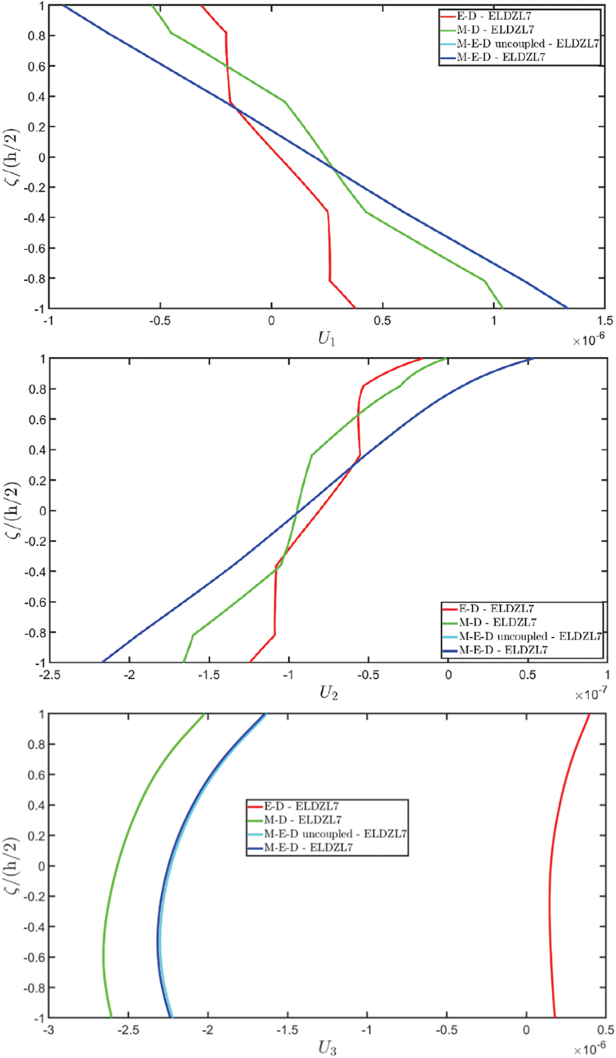
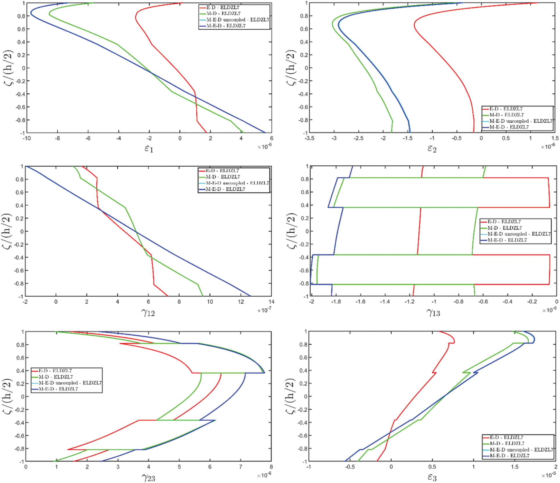
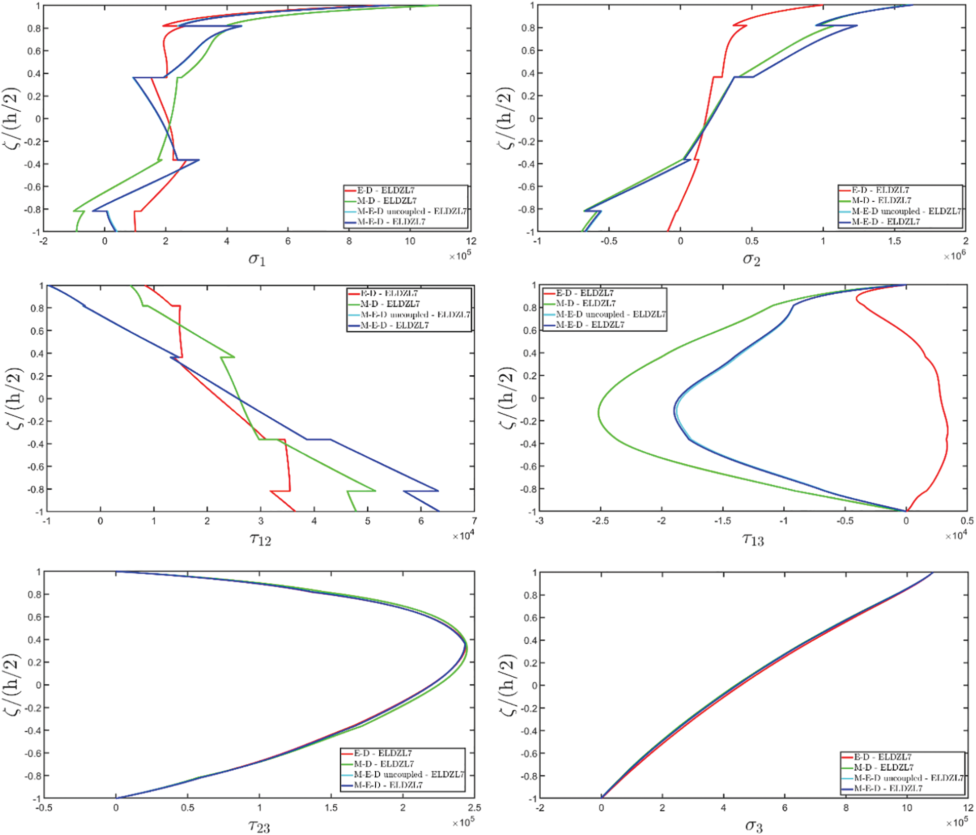


 Copyright © 2025 The Author(s). Published by Tech Science Press.
 Downloads
 Citation Tools