Imbibition Front and Phase Distribution in Shale Based on Lattice Boltzmann Method

1  Introduction

Imbibition is one of the most important mechanisms for the displacement of oil by water in a tight reservoir such as shale in closed time [1,2]. Imbibition may occur as either co-current or counter-current form in the tight reservoir, depending on the boundary conditions and water injection rate. Many experiments on imbibition in tight reservoir cores have been done to investigate the macro process, such as the relation between imbibition length and time. However, it is difficult to observe the movement of fluids among pores and manipulate the porosity, pore scale, and connectivity independently during experiments. An alternative approach is to use advanced simulation tools such as the Lattice Boltzmann Method (LBM), which can provide economic and efficient pathways to investigate the effects of physical and mechanical properties and complex geometry on imbibition [3].

LBM has been used extensively in computational fluid dynamics [4–7]. The lattice Boltzmann equation is a discrete form of the Boltzmann equation and is regarded as a mesoscopic simulation method based on the theory of gas kinetics which can capture the physical phenomena on the mesoscopic scale and translate them into the parameters in macroscopic scale.

LBM has been used in the analysis of ultra-low permeable reservoirs in recent years. The effects of micro characteristic size, boundary layer, and initial water saturation on the imbibition are analyzed [8–11]. Bakhshian et al. [12] studied the effects of the movement of the interface and the effect of roughness on imbibition in a complex pore-fracture structure by using LBM. It is shown that the disorder of the capillary leads to the instability of the interface, which causes the faster development of the front than that predicted by the theoretic model. Hatiboglu et al. [13] simulated the co-current and counter-current imbibition in porous fractural rock by using LBM. The effects of pore size, heterogeneity, and geometric characteristics of the matrix on imbibition were carefully studied.

Most of the former work is based on the assumption in the Lucas-Washburn (L-W) equation where the porous medium is idealized by a bundle of single, straight-line capillaries [14,15], which neither considers the tube wall affects such as roughness, slip nor considers the pressure sensitivity, interaction between pores, two-phase fluid on the same cross-section. Therefore, although these works have made various improvements based on the L-W equation, their application scope in imbibition analysis of tight reservoirs is still limited. In general, these works cannot describe the interaction and heterogeneity between pores and fractures in tight reservoirs.

In this paper, the effects of the main factors on imbibition are analyzed based on the color gradient model of LBM. In the simulation, the distribution of pore size of a core measured by mercury intrusion pores methods is used to build the numerical model. Dimensional analysis was first carried out to obtain the main dimensionless factors. Then LBM is used to simulate the effects of the main dimensionless factors on the imbibition development such as imbibition front, phase distribution, and average imbibition length. The relations between the displacement velocity, displacement efficiency, and the main factors are presented based on the numerical data at last.

2  Color Gradient LBM and Numerical Model

2.1 Simple Introduction of Color Gradient LBM

A two-color nonlinear Boltzmann cell automaton is presented by D’Ortona et al. [16] to study the hydrodynamic problem. This model is improved by Rothman et al. [17], and Gunstensen et al. [18], Latva-Kokko et al. [19]. Later, Leclaire et al. [20] presented a kind of color LBM based on the work of D’Ortona et al. [16] to analyze the immiscible two-phase flow.

In this study, the model provided and improved by Leclaire et al. is chosen to simulate oil displacement by water imbibition [21,22]. The D2Q9 model (a two-dimensional model incorporates nine velocity directions.) is adopted in simulation [23] (Fig. 1).

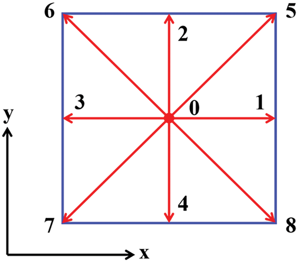
Figure 1: Model of D2Q9 (This is a two-dimensional model that incorporates nine velocity directions. 0~8 indicate the velocity directions)

For a two-phase fluid system, let r indicate the red phase, and b indicate the blue phase. The distribution function is as follows [24]:

fki(x+ci,t+1)=fki(x,t)+Ωki(x,t)(1)

in which i represents either r or b, fki(x+ci,t+1) is the distribution function at time t + 1 and position x + ci, fki(x,t) is the distribution function at time t and position x, collision operator Ωki is adopted as the following form: □

Ωki(x,t)=Ωki3(x,t)[Ωki1(x,t)+Ωki2(x,t)]◻(2)

in which Ωki1 indicates the single-phase operator, i.e., the movement of particles in a single phase induced by the collision among particles. Ωki2 is the perturbation operator, i.e., the interaction among the particles at the interface induced by the interfacial tension. Ωki3 is the re-coloring operator to makes the particles at the interface separate and sends them back to their region.

(1) The collision operator Ωki1

The collision operation of single phase Ωki1 is the same as that in the BGK model which can be expressed as:

Ωki1(x,t)=fki(x,t)−ωk(fki(x,t)−fkie(x,t))(3)

in which ωk is the relaxation factor, fkie is the distribution function at the equilibrium state and is expressed as:

fkie=ρk(ϕik+ωi[3ci⋅u+92(ci⋅u)2−32u2])(4)

in which u is the total local velocity of the two phases, ωi is the weight coefficients, ϕikand ci are both coefficients.

The density of each phase ρk,k=r,b, total density ρ, and total velocity u are expressed as follows:

ρk=∑ifki(5)

ρ=ρr+ρb(6)

u=1ρ∑i∑kfkici(7)

The distribution function at the equilibrium state must assure the conservation of macro mass and momentum, by which the weight coefficients ωi can be determined. The values of ωi in the standard D2Q9 model are determined as follows:

ωi={49i=119i=2,3,4,5136i=6,7,8,9(8)

The values of coefficient ci are determined by:

ci={(0.0)i=0c(cos⁡[(i−1)π2],sin⁡[(i−1)π2])i=1,2,3,42c(cos⁡[(2i−1)π4],sin⁡[(2i−1)π4])i=5,6,7,8(9)

The coefficient ϕik is the function of free parameter αk(k=r,b):

ϕik={αki=11−αk5i=2,3,4,51−αk20i=6,7,8,9(10)

To obtain a stable interface, the density ratio of the two-phase γ should satisfy the following conditions:

γ=ρrρb=1−αbαr(11)

The pressure of each phase is obtained by the following equation:

pk=3ρk(1−αk)5=ρk(csk)2(12)

in which both αb and αr are free parameters, csk is the lattice node sound velocity of the phase k. To avoid the negative pressure, αk≤1 should be ensured. If ρr≥ρb, then the following condition should be satisfied 0≤αb≤αb≤1.

ωi is related to the kinematic viscosity νk: ωi=13νk+0.5. If the viscosities of the two phases are different, ωi at the interface is often determined by interpolation. Therefore, the color field is introduced:

ψ=ρr−ρbρr+ρb(13)

in which ψ is a function ranging from −1 to 1. ψ=1,−1 indicates that the point is occupied by red fluid and blue fluid, respectively. If the value of ψ is in the range (−1, 1), the point is just located at the interface.

The relaxation coefficient ωi is expressed as follows:

ωi={ωrψ>δfr(ψ)α≥ψ>0fr(ψ)0≥ψ≥−δωbψ<−δ(14)

in which δ is a free parameter, where

fr(ψ)=x+ηψ+kψ2(15)

fb(ψ)=x+λψ+νψ2(16)

x=⟨ω⟩,η=2(ωr−x)δ,k=−η2δ,λ=2(x−ωb)δ,ν=−λ2δ(17)

When the viscosities of the two phases are different, the value of δ affects the thickness of the interface. The larger the value of δ is, the larger the thickness of the interface is.

(2) The perturbation operator Ωki2

In the color gradient model, the perturbation operator is used to apply the interfacial tension. The variation degree of color is described by the color gradient F(x) vertical to the interface. F(x) is adopted as follows in this paper:

F(x)=∑ici(ρr(x+ci)−ρb(x+ci))(18)

The perturbation operator is expressed as follows by using F(x):

Ωki2(x,t)=Ak2|F(x)|[Wi(F(x)⋅ci)2|F(x)|2−Bi](19)

in which Ak is the interfacial tension, Bi is:

Bi={−427i=1227i=2,3,4,55108i=6,7,8,9(20)

Though the perturbation operator Ωki2 can characterize the interfacial tension, it cannot ensure that the two phases do not invade each other. Therefore, the re-coloring operator Ωki3 is introduced to let the two phases separate.

(3) The re-coloring operator Ωki3

The function of the re-coloring operator is to send the particles of the two phases in the interface back to their region. Gunstensen et al. [18] and Lin et al. [15] determined the distribution function after the evolution of the re-coloring operator as follows:

W(fri″+fbi″)=max[∑i(fri″−fbi″)ci](21)

meanwhile, the following conditions should be satisfied:

ρr″=∑ifri″=ρr(22)

fri″+fbi″=fi(23)

in which ρr′′ is the density after the re-coloring operation, fri′′,fbi′′ are the distribution functions after the re-coloring operation, ρr and fi are the values before the collision operator. The effects seeking the maximum is to let the direction of color flux H=ρrur−ρbub be the same as the gradient of color F(x) and, so to keep the conservation of the mass of each phase at every lattice node and every direction.

□The computing process of Gunstensen’s model [18] is very complex. Therefore, some researchers presented simplified methods, such as Leclaire et al. [21] gave the following improved operator:

Ωri3(fri)=ρrρfi+βρrρbρ2cos⁡(φi)∑kfkie(ρk,0,αk)(24)

Ωbi3(fbi)=ρrρfi−βρrρbρ2cos⁡(φi)∑kfkie(ρk,0,αk)(25)

in which β is a free parameter, φi is the angle between the color gradient F(x) and the sound velocity of lattice node ci. The distribution function fkie is computed by using the parameters of each phase α, k, and the velocity u = 0. At i = 0, let cos(φi) equal 0. For F(x) = 0, the operator is only computed by the first term. To ensure the value of the distribution function always be positive, the value of β is limited in the range of (0, 1). The smaller the value of β is, the thicker the interface is, and vice versa. It is adopted as 0.999 in the following computation.

2.2 Description of the Numerical Model

(a) Dimensional analysis

The problem considered in this paper is the oil displacement by water due to imbibition. Though the core used for measuring the distribution of pore size is cylindrical, the numerical model is simplified to a planar problem due to the limitation of computer power and considering the symmetry of the sample. The length-to-width ratio of the numerical model is 1:2, the same as that of the length-to-diameter of the core. In the analysis, the parameters of water and oil, pores, capillary and connectivity are considered. They are listed in the following:

The density of oil ρo, viscosity of oil µo, density of water ρw, viscosity of water µw, surface tension σ, contact angle θ, permeability k, porosity ϕ, distribution characteristics such average pore diameter R and standard error for normal distribution, connectivity probability P, earth gravity acceleration g.

At the early and middle stages of imbibition, especially in the case of horizontal imbibition, the earth’s gravity can be neglected. The relation between the radius of pores and the permeability and porosity can be expressed as R2=8kϕ. Use ρw,µw,R to normalize the other parameters, the displacement efficiency η and displacement velocity (imbibition velocity) h˙ can be expressed as follows by taking ρoρw as a constant:

ηh˙u∗}=f(µoµw,µwu∗σcos⁡θ,θ,kR2,α,P)(26)

in which u∗∼µwρwR∼h˙ is the character velocity, µoµw is the viscosity ratio, µwu∗σcos⁡θ is the Ca number, θ is the contact angle or wetting angle, kR2 is the dimensionless permeability, α is the standard error of pore radii, P is the connectivity probability. For a given shale sample, kR2, andα are constants. Then only µoµw,µwu∗σcos⁡θ,θ,P should be considered in the simulation

Previous studies show that the character time tD and character length Lc can be expressed as follows for imbibition in relatively well-distributed and strong wetting rock [25,26]:

tD=tkϕσµoµw1LC2(27)

Similarly, the above Eq. (26) is rewritten as:

ηh˙u∗}=f(kR2σcos⁡θu∗µwµo,P)(28)

(b) The design of the numerical conditions

Based on the above dimensional analysis, the effects of four dimensionless parameters, Ca number (µwu∗σ), θ, µwµo, andP, on the spontaneous imbibition are investigated numerically. Simulation is processed first for a base condition and then for four changed values of each parameter, respectively. In each case, the changed values of one parameter are 80%, 90%, 110%, and 120% of the base value while the other parameters are kept as the base value.

(c) The numerical model and base values of parameters

The distribution of the pore radius used in the simulation is referenced in the measured data of a shale core [27]. The maximum pore radius is 2 μm. The minimum pore radius is 0.125 μm. The pore radii of the core are satisfied with normal distribution. The average pore radius is 9.38×10−2 µm, and the standard error is 2.28×10−2 µm (Fig. 2). For the huge time consumption and the need for storage space during computation by LBM, the calculation area is small. We can think that the pore distribution is symmetric along the long axis in such a size. So we can use a 2D model (a slice of 3D) to simulate. To simulate a larger scale sample, it’d be better to use the upscaling methods or use the actual 3D pore distribution.

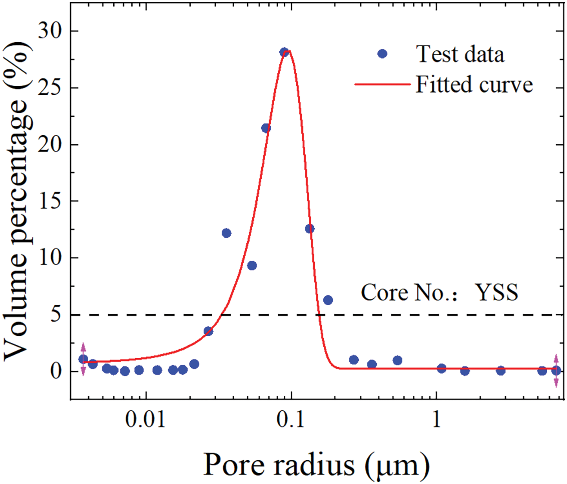
Figure 2: Distribution of pore radius of a shale core by using the nitrogen adsorption method

As for the numerical model, the length of the model is 7.44 μm and the height is 3.435 μm. The length of each throat is 0.315 μm. The upper side and the lower side are impermeable. The right and the left sides are both free and with equal pressure. The right side is surrounded by oil and the left side is surrounded by water. The pores are filled with oil at first. Water is imbibed from the left side while the oil is displaced out from the right side.

The values of parameters for the base model are as follows: the density of water is 1000 kg/m3, the dynamic viscosity of water is 1 mPa·s, the density of oil is 850 kg/m3, the dynamic viscosity of the oil is 5 mPa·s, the contact angle is 36°, the surface tension coefficient is 5.4×10−4N/m. Therefore, the base values of parameters are as follows: Ca=µwu∗σ=2.8×10−2, θ=36∘, µwµo=0.2 andP=100% .

3  Numerical Results and Discussion

3.1 Certification of the Numerical Model and Program

The above equations are programmed in Fortran. To certify the program, the algorithm, and the choice of parameters, the numerical data are compared with experimental results.

Shown in Fig. 3 is the comparison of the numerical results and imbibition experiments using the sample described in Section 2.2 [27]. The dots in the figure are the experimental data and the solid line is the numerical data. It can be seen that the numerical data agrees well with the experimental data. The correlation coefficient is 96%. It is shown that the algorithm and program used in this paper can correctly simulate the flow of two-phase fluids.

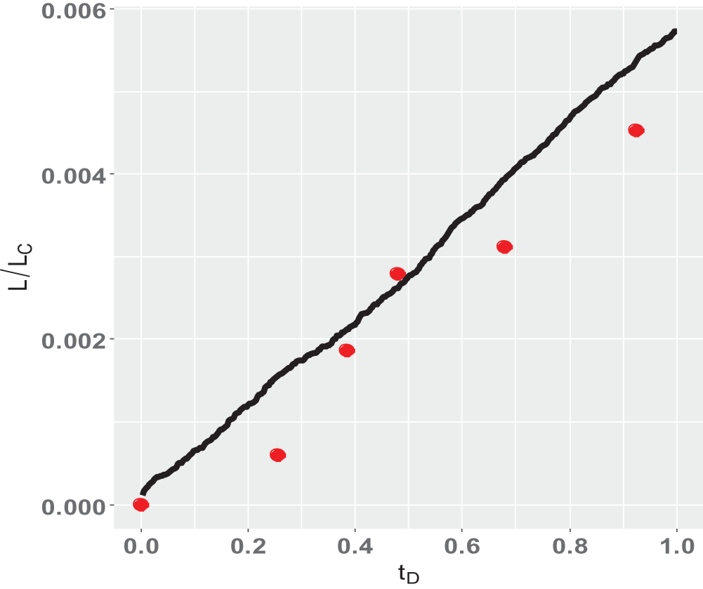
Figure 3: Comparison between simulation results and experimental results of benchmark examples (The dots are the experimental data, and the solid line is the numerical data)

3.2 Distribution of Two-Phase during Imbibition

From the evolution of the distribution of two phases in the pore network, we can see the displacement process, distribution of retained oil, and the displacement interface. Fig. 4 shows the distribution of two phases at four moments. The displace front (interface of oil and water) is not uniform and the heterogeneity enlarges with time. Imbibition develops faster at the upper part than at the lower part. The reason is the heterogeneous distribution of pores. Generally, imbibition develops fast in pores with large size. So along a horizontal line, the imbibition velocities at different positions are varied. The heterogeneity of the imbibition interface cannot be observed in experiments without microobservation. The heterogeneity of the displace interface causes some local pores to be surrounded by water and the oil in these pores is retained. The numerical results show that the assumption of the uniform displacement front during imbibition, used in typical analysis, is not correct for a heterogeneous tight rock.

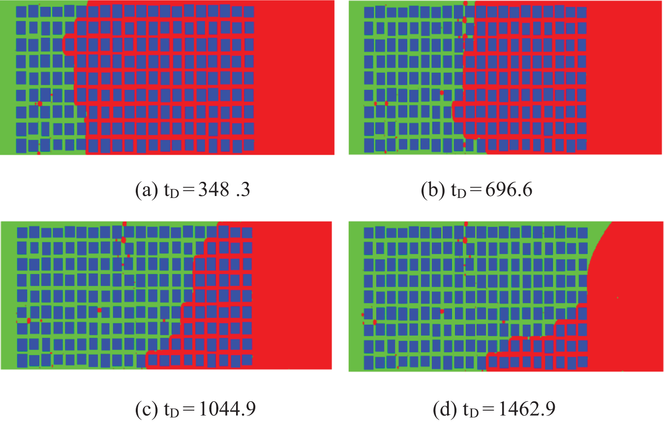
Figure 4: Distribution of two phases with character time tD (The red denotes oil, blue denotes water. Green denotes the shale skeleton. The base values are used in the computation. (a)~(d) show the inhomogeneous development of the imbibition front)

After the water first arrived at the right side, the displace efficiency was 85.25%. This means some oil cannot be displaced in such a heterogeneous network. The displacement efficiency is computed by the way: mass of oil before imbibition-mass of oil after imbibition) mass of oil before imbibition.

In a non-uniformly distributed pore media, the displacement is most unstable due to the capillary fluctuations at the front. The displacement develops into viscous fingering or capillary fingering [28,29]. Therefore, the displacement front almost becomes more and more non-uniform. The displacement front or imbibition front is formed by the positions of all foremost interfaces between oil and water at any given time. To analyze the evolution of the non-uniform degree of the front with time, the standard error of the front positions at different times was computed. Fig. 5 shows that the standard error of the front position increases with time. The scale is 0.83. The wave of interface becomes stronger and stronger with time. The development of imbibition becomes more and more non-uniform. The imbibition in large pores develops faster than in small pores. So, in a rock with distributed random pore size, the evolution of the imbibition is random and the interface becomes more and more irregular, sometimes, fingering occurs, which causes a great decrease in displacement efficiency. By statistically simulating the interface positions of individual pores at various time points during the imbibition process, the standard error of the interface positions at different time points can be obtained. By fitting the standard error of the interface positions to time, their relationship can be derived, as shown in Eq. (29).

Er=5tD0.83(29)

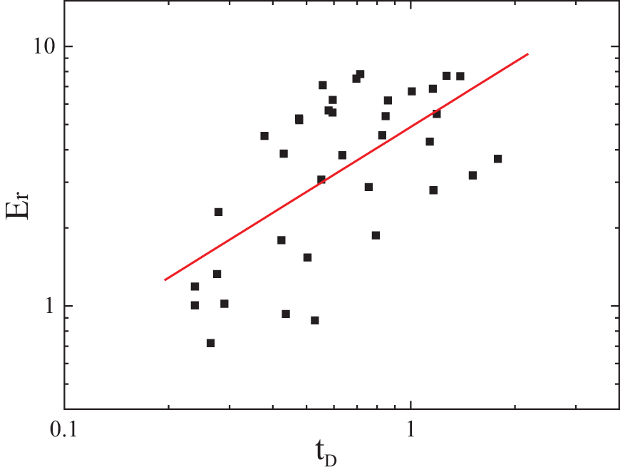
Figure 5: The standard error Er of the interface positions (The interface position means here the distance from the left side to the foremost interface between oil and water at a horizontal line)

3.3 Effects of Factors on the Distribution of Fluid

(a) Effects of Ca number

At different values of Ca, the distribution of retained oil, displacement efficiency and displacement velocity are different from each other though the imbibition processes are similar. At 90% of the base value, the development of imbibition at the upper part becomes faster and faster. The retained oil is mainly located at the lower part (Fig. 6a). At 110% of the base value, most of the oil is displaced out. Only a little oil is retained at the bottom right. The displacement efficiency is high (Fig. 6b). At 120% of the base value (Fig. 6c), the displacement efficiency is larger than that at 90% of the base value but less than that at 110% of the base value. With the decrease of Ca number, the surface tension increase or viscosity decrease, imbibition increases. If the pore size near the upper boundary is relatively large, the imbibition in this area will faster.

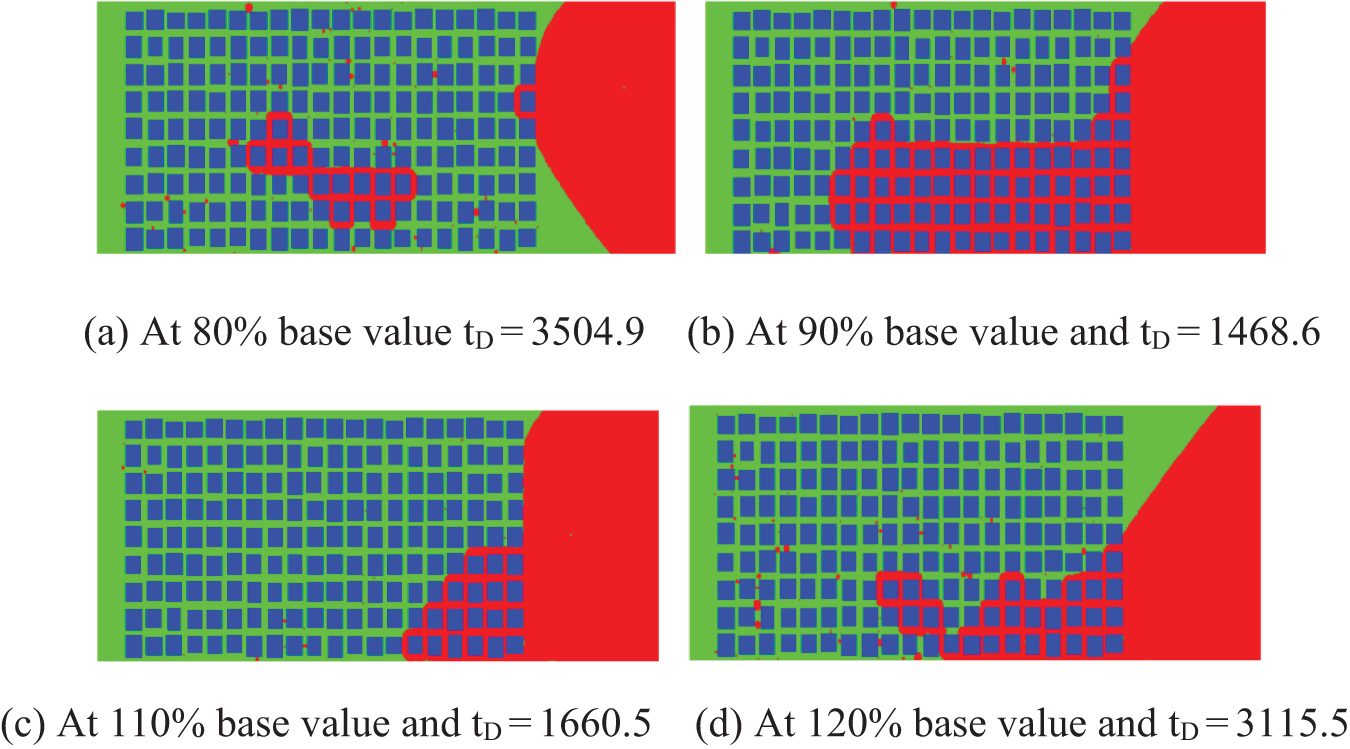
Figure 6: Distribution of oil and water with Ca number

The relation between the displacement efficiency and oil/water viscosity and surface tension is not monotonous. The displacement efficiency increases first and then decreases with the rising of surface tension. In small pores, the surface tension is beneficial for oil displacement by water imbibition. But it is on the contrary in large pores. The displacement efficiency in middle pores is not linear with the surface tension. The results showed also that the effects of Ca number on the displacement efficiency are complicated. The increase of Ca number (e.f., the decrease of surface tension) can on one hand improve the flow of oil drops, but on the other hand can cause the decrease of imbibition force, e.f., drive force of displacement.

(b) Effects of contact angle

When the contact angle is 80% of the base value, the imbibition develops faster near the upper and lower boundary, while the imbibition develops slower, and some oil is retained in the middle part (Fig. 7a). When the contact angle is 90% of the base value, the imbibition develops faster at the upper part than that at the lower part. Much oil is retained at the lower part at last. During the early stage of imbibition, the interface is relatively uniform while it becomes faster and faster at the upper part with time (Fig. 7b). Similar to the early stage of 80% of the base value of contact angle, the imbibition develops faster near the upper and lower boundaries when the contact angle is 110% of the base value. But the difference is the oil in the middle are displaced out and so the retained oil is little in this case (Fig. 7c). When the contact angle is 120% of base value, the imbibition at the upper part becomes faster and faster, which causes much oil to be retained at the lower part (Fig. 7d). It can be found that the effects of contact angle is not monotonous. Its effects are combined strongly with the distribution of pore size, viscosity, and surface tension. For example, the variation of contact angle changes the capillary and the imbibition velocity. Accordingly, the relative permeability will be changed in some pores. Then the mobility ratio (M=Krwµw/Kroµo) may be larger than 1.0, which means the instability of interface (see the discussion in section). The stop and development of instability cause the imbibition very complicated.

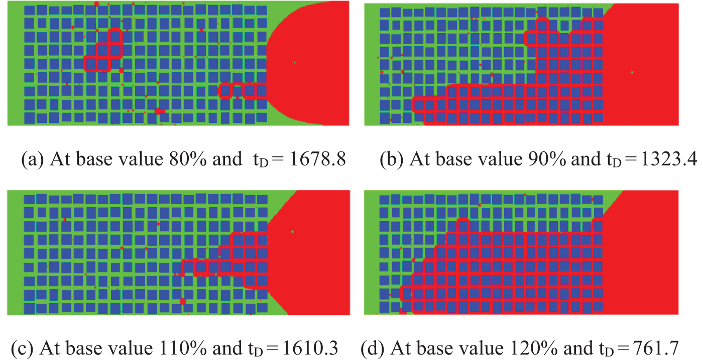
Figure 7: Effects of contact angle on the distribution of oil and water

(c) Effects of viscosity ratio

When the viscosity ratio is 80% of the base value, the development of imbibition is not uniform. At the first stage, the imbibition develops faster at the lower part. At the later stage, imbibition develops upwards. In this case, co-current imbibition accompanies weak counter-current imbibition. There is a small piece of oil retained in the middle near the end. The displacement efficiency is relatively high (Fig. 8a). When the viscosity ratio is 90% of the base value, the development of imbibition is more non-uniform than that at the viscosity ratio of 80% of the base value. Channeling path forms near the upper boundary. Only a little oil is displaced out (Fig. 8b). The development of imbibition is non-uniform both at the viscosity ratio of 110% of the base value and at the viscosity ratio of 120% of the base value, but the displacement efficiency is relatively higher at the viscosity ratio of 110% of the base value (Figs. 8c,d). The viscosity ratio is one of the key factors causing instability of the interface. The variation of viscosity can lead to the formation of a channeling path combined with the distribution of pore size. Once the channeling path is formed, the displacement efficiency decreases greatly.

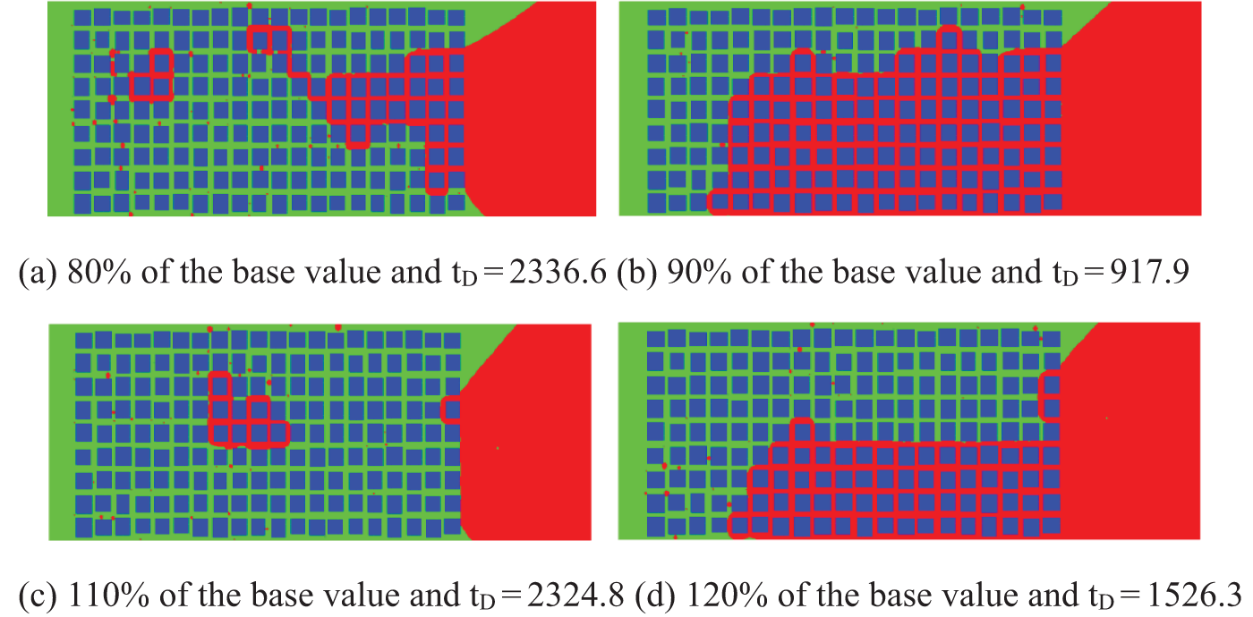
Figure 8: Effects of viscosity ratio on the distribution of oil and water during imbibition

(d) Effects of connectivity

When the connectivity probability is 60% of the base value, imbibition develops very slowly and stops in a short time (Fig. 9a). The imbibition stops at 800 μs and the length is less than 50% of the whole length. The imbibition velocity is faster, and the imbibition length is longer at the connectivity probability of 70% of the base value than at 60% of the base value, but the imbibition front cannot reach the end. The imbibition front stops at 65% of the total length at 350 μs (Fig. 9b). When the connectivity probability is 80%, the imbibition velocity is much faster than that of the first two cases. The imbibition front arrives at the end (Fig. 9c). There is obvious counter-current imbibition in this case. Much oil is retained. The displacement velocity is the fastest at the connectivity probability of 90% but is the most unstable. The channeling path is formed at a later stage. A large piece of oil is retained at the lower right part (Fig. 9d). It is shown that the connectivity probability on the one hand improves the imbibition, on the other hand, leads the interface to be easier to lose instability and increases the retained oil.

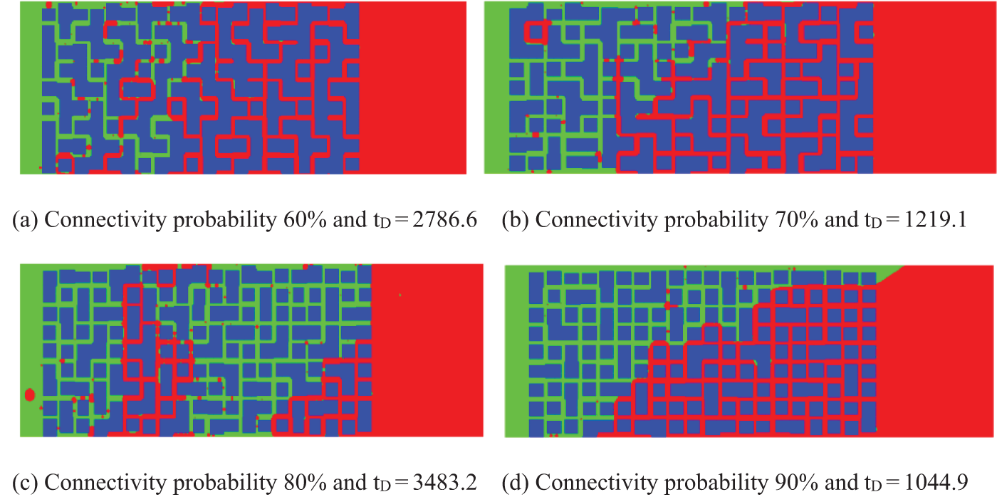
Figure 9: Effects of connectivity probability on the distribution of oil and water

According to the numerical results, it can be seen that the four dimensionless factors (Ca number, θ, µwµo, P) affects imbibition greatly. The effects on either the displacement efficiency or displacement velocity is the comprehensive action of the four factors. Because of the non-uniform distribution of pore size, the imbibition interface does not develop smoothly. In some cases, the channeling path forms and so causes the decrease of displacement efficiency. The reason is that instability of the interface is easy to occur in a non-uniform pore network.

3.4 Development of Imbibition Length

(1) Effects of Ca number

Since the imbibition front is non-uniform, the distance from the left side to the average position of the imbibition front is taken as the imbibition length. Then the slope is the imbibition velocity. Fig. 10 shows the development of imbibition length under different conditions. It can be found that the imbibition length increases with time in a fluctuated way, which is due to the non-uniform distribution of pore size. When water is imbibed into large pores, the velocities will increase fast suddenly and form a footstep. The average displacement velocity of the base model is 18.90 × 10−3 m/s. When Ca are 80%, 90%, 110%, and 120% of the base value, the average displacement velocities are 8.72 × 10−3 m/s, 12.14 × 10−3 m/s, 13.18 × 10−3 m/s and 7.67 × 10−3 m/s (Fig. 10a), and the corresponding displacement efficiencies are 87.22%, 61.03%, 87.77%, and 80.56%, respectively. The decrease of Ca number means the relative increases of imbibition force or the decrease of viscous resistance. However, the effect of Ca number on imbibition is not monotonous. Generally, with the increase of Ca, the development of imbibition becomes slow. In the first stage, the imbibition curves are very close when Ca equals 80%, 90% of the base value. The curves when Ca equals 110% and 120% of the base value become obvious relative to the other three cases. It means that the development of imbibition cannot be determined by Ca number only.

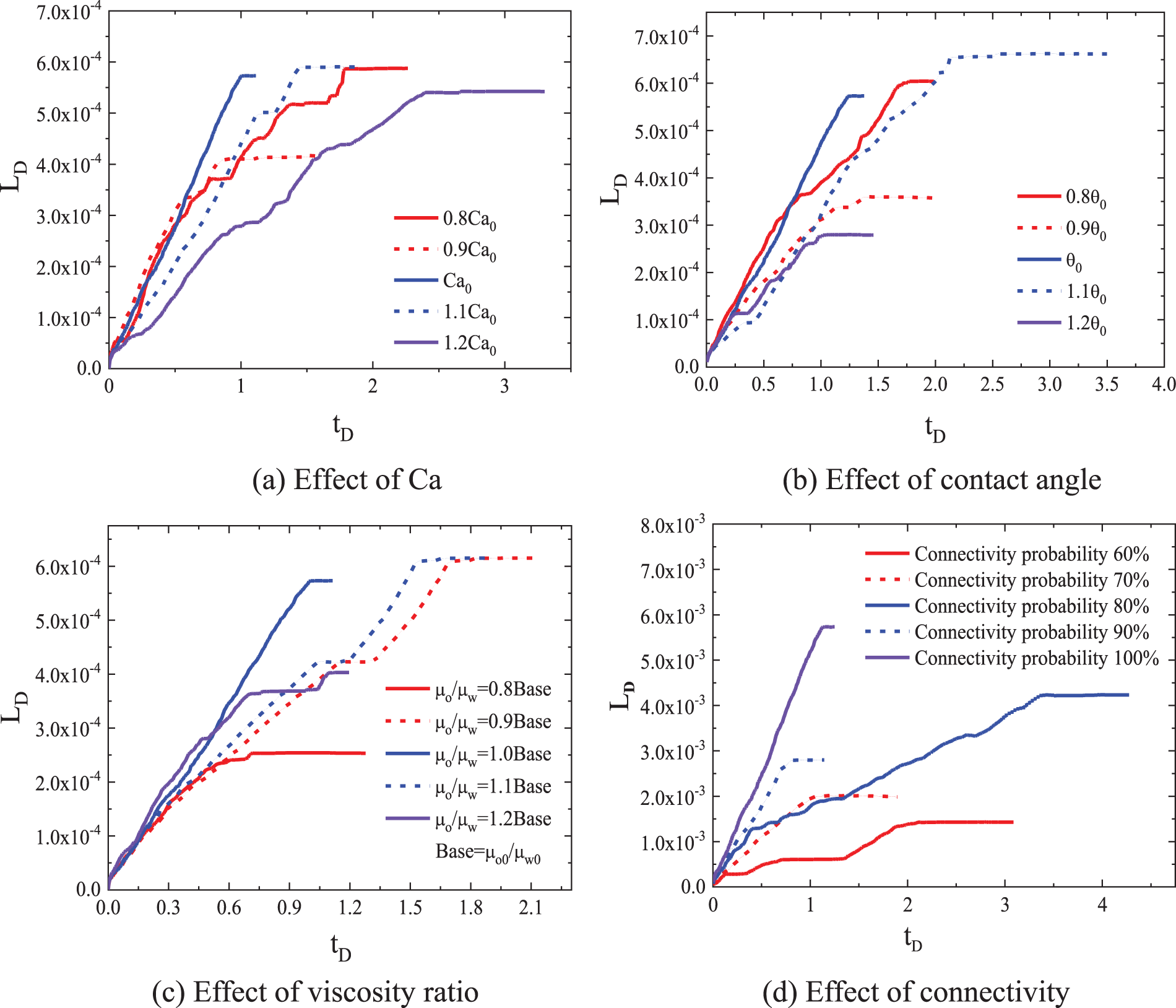
Figure 10: Effects of factors on the development of imbibition length with time. (a) Variation of imbibition length with Ca number (Ca0 means the base value of Ca number. LD=h/Lc); (b) Variation of imbibition length with contact angle (θ0 means the base value of contact angle; (c) Variation of imbibition length with viscosity ratio; (d) Variation of imbibition length with connectivity)

(2) Effects of contact angle

Imbibition develops slowly with the increase of the contact angle. When the contact angles are 80%, 90%, 110%, and 120% of the base value, the displacement efficiencies are 89.96%, 53.54%, 98.44%, and 41.49%, and the average displacement velocities are 13.14 × 10−3, 9.80 × 10−3, 8.96 × 10−3 and 7.83 × 10−3 m/s, respectively (Fig. 10b). Similar to the effects of Ca number, the displacement efficiency and velocity do not change with contact angle monotonously.

The contact angle reflects the wettability of materials. The larger the contact angle is, the lower the wettability and the capillary are, and the meantime the smaller the size of the oil drop is. So the increase in contact angle is not beneficial to displacement. In practice, surfactant is often adopted to change the wettability. Meanwhile, the permeability is changed with surfactant also. So the displacement efficiency is determined by two aspects when adopting surfactant [30,31].

(3) Effects of viscosity ratio

When the viscosity ratios are 80%, 90%, 110%, and 120% of the base value, the corresponding displacement efficiencies are 93.39%, 37.66%, 91.25%, and 59.78%, and the average displacement velocities are 8.19 × 10−3, 12.84 × 10−3, 11.39 × 10−3, and 9.77 × 10−3 m/s, respectively. The displacement efficiency does not change with the viscosity monotonously also (Fig. 10c). The viscosity ratio has great effects on the instability of the imbibition interface. This factor causes the wave change of the curve of the imbibition length with time [32].

(4) Effects of connectivity probability

Through several test simulations with different connectivity, it is found that the connectivity of the pore network model used in this paper cannot be lower than 50%. When the connectivity is equal to or less than 50%, it is very difficult to form a passage for liquid to pass between the left and right sides of the pore network. Obviously, in this case, the oil in the pore network cannot be displaced to the right out of the pore network. So, the connectivity probabilities of 60%, 70%, 80%, and 90% are adopted in the numerical simulation.

When the connectivity probabilities are 60% and 70%, respectively, the imbibition velocity and the swept area are both small. The displacement velocities are faster when the connectivity probabilities are adopted as 80% and 90% (Fig. 10d). The retained oil is larger at the connection probability of 80% than at 90%, but smaller than that at connectivity probabilities of 60% and 70%.

According to the numerical results, it can be seen that the four dimensionless factors (Ca number, θ, µwµo, P) affect imbibition greatly. The effects on either the displacement efficiency or displacement velocity are the comprehensive action of the four factors. Because of the non-uniform distribution of pore size, the imbibition interface does not develop smoothly. In some cases, the channeling path forms and so causes a decrease in displacement efficiency. The reason is that instability of the interface is easy to occur in a non-uniform pore network.

3.5 The Relation Between Displacement Efficiency, Displacement Velocity, and the Four Main Factors

To compare the effects of the four factors on the displacement efficiency and the displacement velocity, the sensitivity of each factor (the change of the displacement efficiency or the displacement velocity/changes of each factor from the base value to 90% of the base value) is investigated as shown in Fig. 11. The effects of the connectivity probability on the imbibition velocity is the largest while the effects of contact angle are the smallest. The effects of Ca number on the displacement efficiency is the largest.

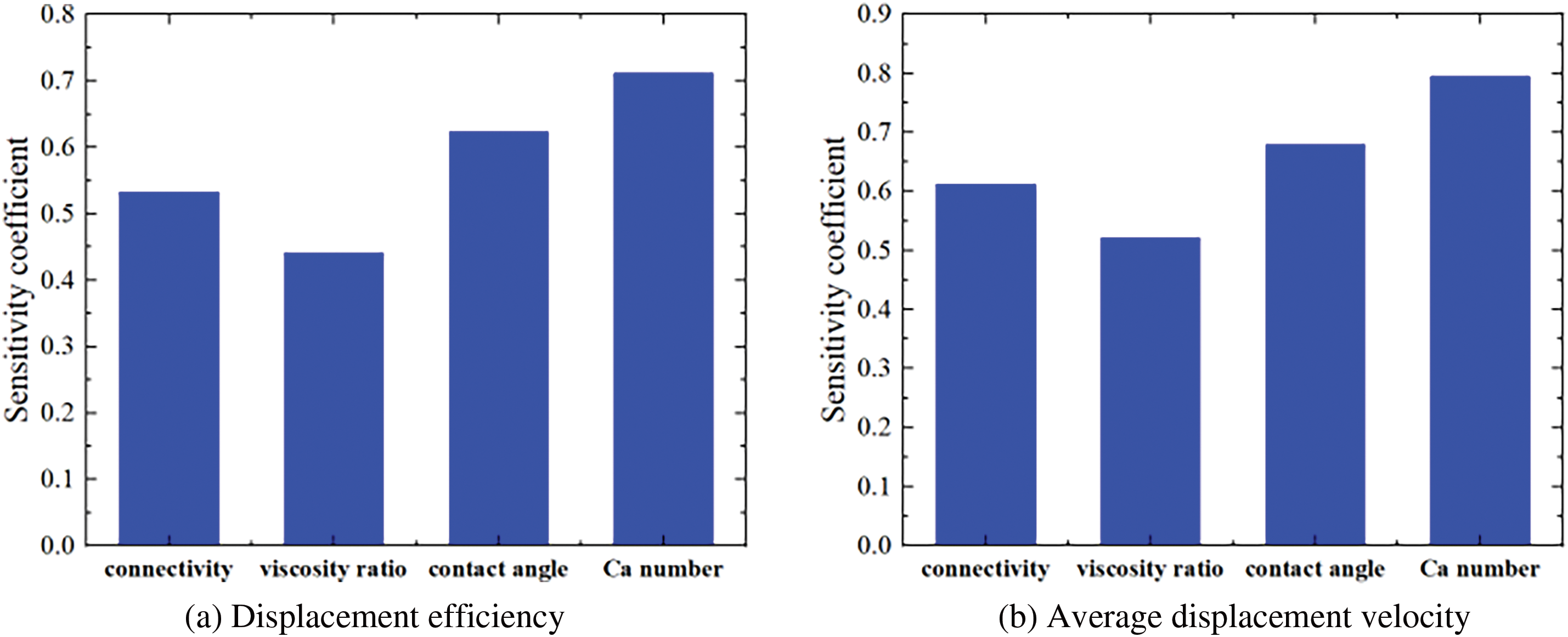
Figure 11: Sensitivity of factors on displacement efficiency and average displacement velocity

Displacement efficiency is the value of displaced oil divided by the total oil; Because the imbibition front is not uniform, average displacement velocity is used to characterize the imbibition progress which equals the average position of the front divided by time.

In Section 2.2 (a), we obtained the theoretical relations between the imbibition velocity and displacement efficiency and two dimensionless parameters (Eq. (28)). Here, based on the numerical data, the specific expressions of Eq. (28) are obtained. During fitting, the relations were assumed to be exponential. The relations between displacement efficiency, average displacement velocity, and the four main factors are fitted by using the least square method (Eqs. (30) and (31)). The predicted data based on the fitted relations and the numerical data are shown in Fig. 12. It is shown that the predicted data and numerical data agree with each other.

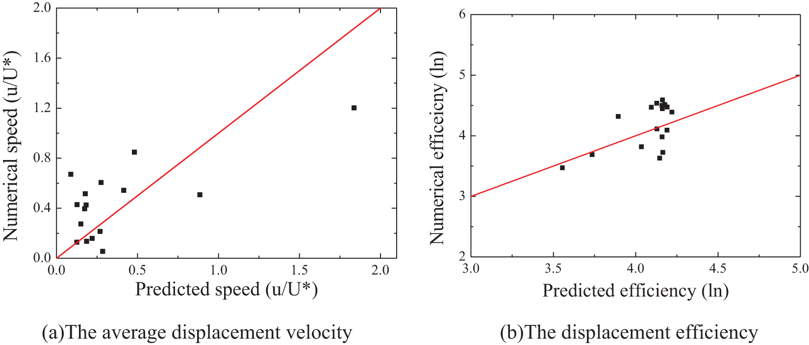
Figure 12: Comparison between the predicted value and the numerical value

The fitted equation of the average displacement velocity:

h˙u∗=0.05P−19.73(σcos⁡θu∗µwµo)19.36(30)

The fitted equation of the displacement efficiency:

η=0.98P1.34(σcos⁡θu∗µwµo)3.76(31)

The horizontal coordinate denotes the predicted value, and the vertical coordinate denotes the numerical value. The solid line denotes all the dots that the predicted value equals the numerical value. The closer the dot to the solid line is, the more exact the predicted value is.

4  Conclusions

LBM was used to simulate the effects of main factors on oil displacement by water imbibition. The numerical model was built by referencing the distribution of pore size of a shale core. Four main dimensionless factors (Ca number, θ,µwµo, and P)are obtained by dimensional analysis. From the simulation results, the following conclusions can be drawn:

1. The oil is displaced by water imbibition. The four factors have huge effects on imbibition. The impact of each factor is not monotonous. The displacement process is the comprehensive effect of all aspects.

2. From the point of sensitivity, the connectivity probability has the greatest effect on the average displacement velocity while the contact angle has the smallest one. As for the displacement efficiency, the effect of the Ca number is the largest. Based on the numerical data, the fitted relations between the displacement efficiency, average displacement velocity, and the four factors are obtained.

In this work, only a kind of distribution of pore size and four dimensionless factors are considered. Displacement by imbibition is related to many other factors as well, such as variation in the distribution of pore size, properties of liquid for imbibition, and external pressure. The effects of these factors are required to be studied further in the future. Meanwhile, considering the large amount of time consumption and the need for storage space during computation by LBM, our analysis is only on a small-scale zone considering pore-size distribution from a shale sample. In future work, we will use a larger scale in numerical simulation.

Acknowledgement: Thank Yingjun Li for his help in discussing LBM and Liu Yang for providing some shale samples for parameter test.

Funding Statement: This work was supported by the National Natural Science Foundation of China (12072347); the Excellent Training Plan of the Institute of Mechanics, Chinese Academy of Sciences; and CNPC New Energy Key Project (2021DJ4902).

Author Contributions: Conceptualization, Xiaobing Lu; Programming and simulation, Li Lu, Xuhui Zhang; Manuscript writing, Li Lu, Yadong Huang; and Kuo Liu collected data and rock samples. All authors reviewed the results and approved the final version of the manuscript.

Availability of Data and Materials: The data that support the findings of this study are available from the corresponding author, Xiaobing Lu, upon reasonable request.

Ethics Approval: Not applicable.

Conflicts of Interest: The authors declare no conflicts of interest to report regarding the present study.

References

1. Wang H, Su YL, Wang WD. Investigations on water imbibition into oil-saturated nanoporous media: coupling molecular interactions, the dynamic contact angle, and the entrance effect. Indust Eng Chem Res. 2021;60(4):1872–83. doi:10.1021/acs.iecr.0c05118. [Google Scholar] [CrossRef]

2. Yang L, Gao JW, Zheng Y, Li X, Zhang Y. Numerical simulation of imbibition law of heterogeneous sandy conglomerate: lattice boltzmann method. Chin J Comput Phys. 2021;38(5):534–42. doi:10.19596/j.cnki.1001-246x.8346. [Google Scholar] [CrossRef]

3. Zhang S, Li J, Coelho RCV, Wu K, Zhu Q, Guo S, et al. Lattice Boltzmann modeling of forced imbibition dynamics in dual-wetted porous media. Int J Multiphase Flow. 2024;182:105035. doi:10.1016/j.ijmultiphaseflow.2024.105035. [Google Scholar] [CrossRef]

4. Liu Y, Zhu R, Qin X, Zhou Y, Sun Q, Zhao J. Numerical study of capillary-dominated drainage dynamics: influence of fluid properties and wettability. Chem Eng Sci. 2024;291:119948. doi:10.1016/j.ces.2024.119948 [Google Scholar] [CrossRef]

5. Zakirov TR, Khayuzkin AS, Khramchenkov MG, Galeev AA, Kosterina EA. Effect of gravity number on soil contamination during dynamic adsorption of heavy metal ions: a lattice Boltzmann study. Int Commun Heat Mass Transfer. 2024;158:107852. [Google Scholar]

6. Wu S, Wu J, Liu Y, Yang X, Zhang J, Zhang J, Zhang D, Zhong B, Liu D. Lattice Boltzmann modeling of the coupled imbibition-flowback behavior in a 3D shale pore structure under reservoir condition. Front Earth Sci. 2023;11:1138938. doi:10.3389/feart.2023.1138938. [Google Scholar] [CrossRef]

7. Guo ZL, Zhao TS, Shi Y. Physical symmetry, spatial accuracy, and relaxation time of the lattice Boltzmann equation for micro gas flows. J Appl Phys. 2006;99(7):74903–17. doi:10.1063/1.2185839. [Google Scholar] [CrossRef]

8. Wang H, Cai JC, Su YL, Jin ZH, Zhang MS, Wang WD, et al. Pore-scale study on shale oil-CO2–water miscibility, competitive adsorption, and multiphase flow behaviors. Langmuir. 2023;39(34):12226–34. [Google Scholar] [PubMed]

9. Abubaker M, Sohn CH, Ali HM. Wetting performance analysis of porosity distribution in NMC111 layered electrodes in lithium-ion batteries using the Lattice Boltzmann Method. Energy Rep. 2024;12:2548–59. doi:10.1016/j.egyr.2024.07.020. [Google Scholar] [CrossRef]

10. Wang N, Kuang T, Liu Y, Yin Z, Liu H. Wetting boundary condition for three-dimensional curved geometries in lattice Boltzmann color-gradient model. Phys Fluids. 2024;36(3):032133. doi:10.1063/5.0200478. [Google Scholar] [CrossRef]

11. Cheng Z, Gao H, Tong S, Zhang W, Ning Z. Pore scale insights into the role of inertial effect during the two-phase forced imbibition. Chem Eng Sci. 2023;278:118921. [Google Scholar]

12. Bakhshian S, Murakami M, Hosseini SA, Kang QJ. Scaling of imbibition front dynamics in heterogeneous porous media. Geophys Res Lett. 2020;47(14):e2020GL087914. doi:10.1029/2020GL087914. [Google Scholar] [CrossRef]

13. Hatiboglu CU, Babadagli T. Pore-scale studies of spontaneous imbibition into oil-saturated porous media. Phys Rev E. 2008;77:066311. [Google Scholar]

14. Lucas R. Rate of capillary ascension of liquids. Kolloid-Zeitschrift. 1918;23(1):15–22. [Google Scholar]

15. Lin CD, Xu AG, Zhang GC, Li YJ. Polar coordinate lattice Boltzmann shocking process—investigation of non-equilibrium effects in complex system. Adv Condens Mater Phys. 2013;2:88–96. [Google Scholar]

16. D’Ortona U, Salin D, Cieplak M, Rybka RB, Banavar JR. Two-color nonlinear Boltzmann cellular automata: surface tension and wetting. Phys Rev E. 1995;51(4):3718–28. doi:10.1103/PhysRevE.51.3718. [Google Scholar] [PubMed] [CrossRef]

17. Rothman DH, Keller JM. Immiscible cellular-automation fluids. J Sta Phys. 1998;52(3/4):119–27. doi:10.1007/BF01019743. [Google Scholar] [CrossRef]

18. Gunstensen AK, Rothman DH, Zaleski S, Gianluigi Z. Lattice Boltzmann model of immiscible fluids. Phys Rev A. 1991;43(8):4320–7. doi:10.1103/PhysRevA.43.4320. [Google Scholar] [PubMed] [CrossRef]

19. Latva-Kokko M, Rothman DH. Diffusion properties of gradient-based lattice Boltzmann models of immiscible fluids. Phys Rev. 2005;E71:056702. doi:10.1103/PhysRevE.71.056702. [Google Scholar] [PubMed] [CrossRef]

20. Leclaire S, Reggio M, Trépanier JS. Numerical evaluation of two recoloring operators for an immiscible two-phase flow lattice Boltzmann model. Appl Math Model. 2012;36(5):2237–52. doi:10.1016/j.apm.2011.08.027. [Google Scholar] [CrossRef]

21. Leclaire S, Pellerin N, Reggio M, Jean Y. Multiphase flow modeling of spinodal decomposition based on the cascaded lattice Boltzmann method. Phys A Statist Mech Its Appl. 2014;406(10):307–19. doi:10.1016/j.physa.2014.03.033. [Google Scholar] [CrossRef]

22. Leclaire S, Pellerin N, Reggio M, Trépanier JY. Enhanced equilibrium distribution functions for simulating immiscible multiphase flows with variable density ratios in a class of lattice Boltzmann models. Int J Multiphase Flow. 2013;57:159–68. doi:10.1016/j.ijmultiphaseflow.2013.07.001. [Google Scholar] [CrossRef]

23. Qian YH, D’Humieres D, Lallemand P. Lattice BGK models for Navier-stokes equation. Europhys Lett. 1992;17(6):479–84. doi:10.1209/0295-5075/17/6/001. [Google Scholar] [CrossRef]

24. Yao Q. Lattice Boltzmann method for the simulation of two-phase flow based on the RK model [thesis for master degree]. Shanghai, China: East China University of Science and Technology; 2017 (In Chinese). [Google Scholar]

25. Ma S, Morrow NR, Zhang X. Generalized scaling of spontaneous imbibition data for strongly water-wet systems. J Pet Sci Eng. 1997;18(3-4):165–78. doi:10.1016/S0920-4105(97)00020-X. [Google Scholar] [CrossRef]

26. Yang L, Ge H, Shi X, Cheng Y, Zhang K, Chen H, et al. The effect of microstructure and rock mineralogy on water imbibition characteristics in tight reservoirs. J Natural Gas Sci Eng. 2016;34(2):1461–71. doi:10.1016/j.jngse.2016.01.002. [Google Scholar] [CrossRef]

27. Lu L. Study on characteristic experiment and LBM numerical simulation of spontaneous imbibition in tight oil and gas reservoirs [Ph.D. thesis]. Beijing, China: China University of Mining & Technology-Beijing; 2022 (In Chinese). [Google Scholar]

28. Méheeust Y, Løvoll G, Mäløy KJ. Interface scaling in a two-dimensional porous medium under combined viscous, gravity, and capillary effects. Phys Rev E. 2002;66(5):051603. doi:10.1103/PhysRevE.66.051603. [Google Scholar] [PubMed] [CrossRef]

29. Ju Y, Gong WB, Chang W, Sun M. Effects of pore characteristics on water-oil two-phase displacement in non-homogeneous pore structures: a pore-scale lattice Boltzmann model considering various fluid density ratios. Int J Eng Sci. 2020;154:103343. [Google Scholar]

30. Lu L, Li YJ, Zhang XH. Effects of cracks and geometric parameters on the flow in Shale. ACS Omega. 2021;6(7):4619–29. [Google Scholar] [PubMed]

31. Warda HA, Haddara SH, Wahba EM, Sedahmed M. Lattice Boltzmann simulations of the capillary pressure bump phenomenon in heterogeneous porous media. J Petrol Sci Eng. 2017;157:558–69. doi:10.1016/j.petrol.2017.06.058. [Google Scholar] [CrossRef]

32. Liu HH, Zhang YH, Valocchi AJ. Lattice boltzmann simulation of immiscible fluid displacement in porous media: homogeneous versus heterogeneous pore network. Phys Fluids. 2015;27:052103. doi:10.1063/1.4921611. [Google Scholar] [CrossRef]