Sensitivity Analysis of Structural Dynamic Behavior Based on the Sparse Polynomial Chaos Expansion and Material Point Method

1  Introduction

In practical engineering, structures are often subjected to dynamic loads such as impact loads and vibration loads. With the increasing demands for safety and reliability in fields like mechanical, civil, and military engineering, accurately assessing the effects of these dynamic loads on structures has become a critical issue [1,2]. However, experimental studies on these responses are usually costly, and time-consuming, and the results are often difficult to predict accurately. For this reason, a variety of numerical simulation methods [3,4] have been applied to the engineering field with successful results. Among them, the material point method (MPM) proposed by Sulsky et al. [5,6] has been proven to have high accuracy in dealing with institutional dynamics problems such as extreme deformation, which is a meshless method based entirely on Lagrangian particles and avoids the mesh distortion problem inherent to the Lagrangian method in deformation calculations by combining the advantages of the Lagrangian method and Eulerian method. In recent years, Zhang et al. [7] proposed the material point finite element method based on the two methods for accurately dealing with deformation problems, and developed MPM3D, a three-dimensional explicit parallel material point method numerical simulation software for impact explosion problems. Lian et al. [8] introduced finite elements into MPM and proposed the hybrid material point finite element method. In addition, scholars have proposed an adaptive split-mass scheme for MPM [9] and established a contact algorithm based on localized multiple background grids [10], all of which are improving the simulation accuracy.

In structural dynamics, there are multiple sources of uncertainty associated with structural model properties, including random variations in material properties, load variations, etc. Therefore, the effect of uncertainty in structural parameters on the properties of structural dynamics is important [11,12]. Structural dynamics sensitivity analysis is a method for assessing the sensitivity of the dynamic properties of a structural system to changes in design parameters, which includes local sensitivity analysis (LSA) and global sensitivity analysis (GSA). Some of the sensitivity analysis methods are the global finite difference method (FDM) [13], Morris method [14], fourier amplitude sensitivity test (FAST) [15], and Sobol method [16] based on variance decomposition. In particular, the FDM and Sobol methods have higher accuracy in dealing with nonlinear systems such as structural dynamics.

Sensitivity analysis [17,18] of structural dynamics has traditionally been conducted using finite element methods. However, for deformation problems, MPM has high accuracy, but MPM simulations are computationally expensive and therefore less suitable for large-scale fast iterative calculations. This limitation restricts the broader application of MPM in sensitivity analysis, particularly when a high number of iterations is required for the comprehensive exploration of parameter spaces. To reduce the computational cost of the MPM, Dong et al. [19] use multiple GPUs to parallelize the MPM, Wang et al. [20] use a GPU acceleration framework coupled with MPM, Zeng et al. [21] propose an adaptive peridynamics MPM, and Huang et al. [22] proposed an MPM parallel algorithm for shared memory computers based on OpenMP, all of which improve the computational efficiency. All these methods can improve the computational efficiency of MPM, but they are still inefficient for the large number of samples required for sensitivity analysis. Therefore, the contribution of this paper is to present the construction of a response surface model (e.g., support vector machine (SVM) [23], decision tree (DT) [24], Gaussian process regression (GPR) [25], polynomial chaos expansion (PCE) [26], etc.) as a surrogate model for MPM, which enables efficient Monte Carlo simulation.

Response surface methods involve two types of numerical errors, the Monte Carlo error (which converges to zero when the sample size is infinite), and the error between the alternative model and the real physical model, which significantly affects the computation of local and global sensitivities. In recent years, the PCE model has been widely used in sensitivity analysis because it can avoid the first type of errors and improve computational accuracy. The advantage of PCE is that it can perform both local and global sensitivity analysis, including Sobol indices [27] which can be derived directly from PCE coefficients [28] or even distribution-based sensitivity indices [29] derived from PCE [30], it is possible to analytically obtain derivatives of PCE [31]. However, this approach will face a serious “curse of dimension” problem when confronted with high-dimensional and high-order PCE. To overcome this difficulty, Blatman et al. [32] proposed a sparse PCE method, which uses adaptive least squares regression or minimum angle regression to retain the main variance contributors in the PCE, and avoids solving the coefficients of all the PCE expansion terms. The main difference between sPCE and traditional PCE lies in sparsity. The sPCE model reduces computational complexity and the number of required samples by selecting the most important polynomial basis functions, thereby improving efficiency. The benefits of using the sPCE model include faster computation speed, lower memory usage, and higher accuracy when dealing with high-dimensional uncertainties. In addition, some scholars have used more advanced sampling techniques to efficiently construct PCE, e.g., active learning further reducing the number of samples [33,34] or adaptive stochastic domain decomposition (multi-element PCE) [30]. In the process of determining the basis functions, researchers have proposed greedy algorithms such as orthogonal matching pursuit (OMP) [35] and randomized greedy algorithm (RGA) [36], all of which improve the accuracy of sPCE. The second type of error mainly depends on the order of the polynomial expansion, and the error decreases with the increase of the order, but the efficiency also decreases, so the contribution of this paper is to present an approach that balances the accuracy and the efficiency to reduce the second type of error and thus to obtain the accurate sPCE.

In this paper, several classical examples of structural dynamics are selected for sensitivity analysis tests. The response surface models are constructed to replace the MPM physical model to improve the computational efficiency and reduce the Monte Carlo error. Based on RGA, the coefficient of variation [37] is introduced as an adaptive termination condition for polynomial order selection, to obtain an accurate sPCE surrogate model and reduce the error between the alternative model and the real physical model. The FDM and Sobol methods are introduced to compute local and global sensitivities based on the sPCE model to improve the accuracy and completeness of the results. In brevity, the innovations of this paper are as follows:

•   The MPM is used for sensitivity analysis of structural dynamics.

•   Response surface model is constructed to replace the MPM-based physical model.

•   Adaptive RGA is used to obtain an accurate sPCE model.

•   Local and global sensitivity analysis of structural dynamics based on sPCE.

The remaining structure of this paper is outlined as follows: Section 2 introduces the analytical process of the MPM utilized for computing various output parameters in the case studies presented in this paper. Section 3 describes the principles of sPCE and the process of solving for local and global sensitivities. Section 4 validates the proposed methods’ accuracy and effectiveness through numerical examples. Finally, Section 5 provides concluding observations.

2  Structural Dynamics Analysis by Material Point Method

The material point method (MPM) uses two types of discretization: background mesh discretization, which solves the discrete governing equations, and material point discretization, which defines the object’s geometrical configuration and the physical quantities it contains. The method combines the best of Eulerian and Lagrangian approaches by storing physical information on material points, employing Lagrangian material points to track material interfaces, and introducing an intrinsic model related to the deformation history. An interpolation function transfers physical information from material points to background nodes, and the equilibrium equations are computed on the background mesh. Mesh distortion is prevented due to the steady backdrop mesh.

As shown in Fig. 1, the computational process of MPM is divided into four steps: First, the background mesh is defined and the mass, momentum, and internal force terms of all the mass points are mapped to the background mesh nodes. Second, the physical information carried by the material points is mapped to the background grid through shape function interpolation, updating the momentum and displacement information of the background grid nodes. Third, the velocity and acceleration fields of the background mesh nodes are used to update the positions and velocities of the particles, the nodal velocity fields are utilized to calculate the strain increments and spin increments, and the stresses are updated according to the constitutive equations. Fourth, the updated grid is reset—it is this step that renders MPM free of mesh distortion.

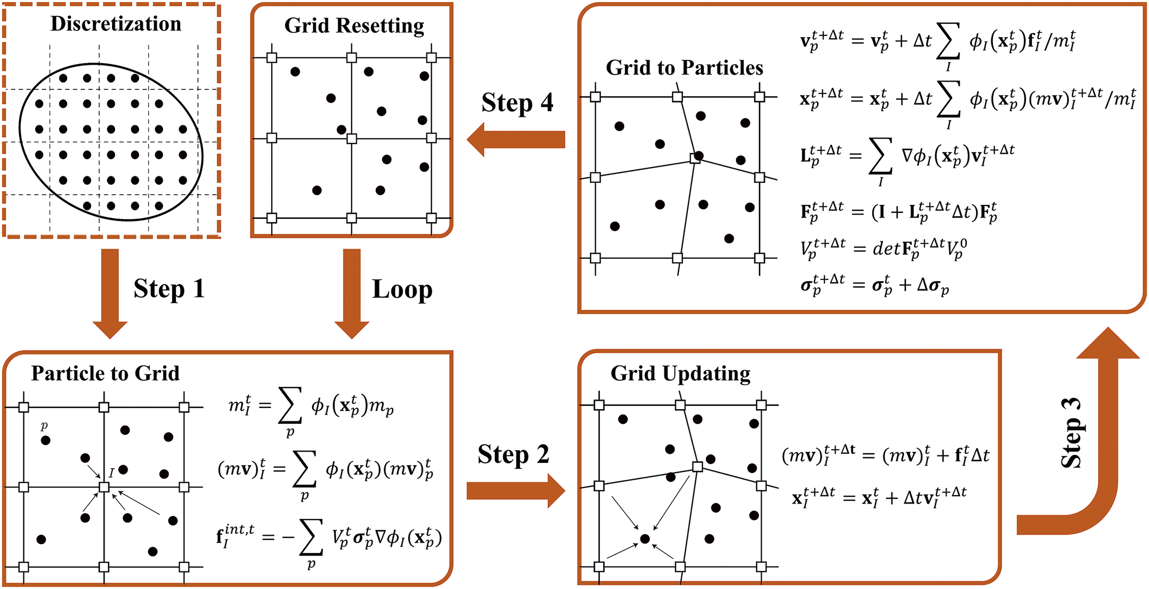
Figure 1: Typical particle discretization and solution steps for 2D material domains

Within the framework of the updated Lagrangian description, the momentum balance equation is expressed as follows:

ρdvdt=∇⋅σ+ρb(1)

where v(x,t)=du(x,t)/dt stands for velocity and ρ(x,t) for mass density. b(x,t) is the particular body force, and σ(x,t) is the Cauchy stress tensor. The particle’s coordinates at time t are indicated by the vector x. To obtain a solution to the momentum balance equation, the following boundary and starting conditions must be satisfied:

σ(x,t)⋅n|Γt=t¯(t),u(x,t)|Γu=u¯(t)(2)

u(x,0)=u0(x),v(x,0)=v0(x)(3)

where Γt is the portion of the boundary with a prescribed traction vector t¯, Γu is the boundary with a prescribed displacement u¯, and n is the outward normal to the surface Γt. u0(x) and v0(x) stand for the initial displacement and velocity, respectively. One way to express the Galerkin weak form of Eq. (1) is

∫Vρu¨⋅wdV+∫Vσ:∇wdV−∫Vρw⋅bdV−∫Γtw⋅t¯dΓ=0(4)

where w∈R0, R0={w|w∈C0,w|Γy=0} stands for the test function and V for the continuum’s current configuration. Given that np particles describe the entire domain, the mass density can be roughly expressed as

ρ(x,t)=∑p=1npmpδ(x−xpt)(5)

where the mass of particle p is represented by the symbol mp, the Dirac delta function is marked by δ, and the current position of particle p at time t is indicated by xpt. By inserting Eq. (5) into Eq. (4), the integral is converted into a quantity that needs to be added up at the particle:

∑p=1npmpu¨p⋅wp+∑p=1npmpρpσp:∇wp−∑p=1npmpbp⋅wp−∑p=1npmpρpht¯p⋅wp=0(6)

where h denotes the thickness of the boundary layer and u¨p denotes the acceleration of the particle p.

In the three-dimensional problems, the background grid is constructed using hexahedral elements with eight nodes. The particles are labeled with the subscript index p, while the nodes of the background grid are labeled with the subscript index I. The node shape function of the 8-node cell is defined as

NI=18(1+εεI)(1+ηηI)(1+ζζI),I=1,2,…,8(7)

where εI,ηI and ζI are the natural coordinates (±1) at node I. Thus, uI and the test function wI can represent the displacement of any particle in the cell as follows:

up=∑I=1ngNIpuI,wp=∑I=1ngNIpwI(8)

where the value of the shape function evaluated at particle p concerning node I is denoted as NIp=NI(xp). The total number of nodes in the background grid is represented by ng.

By replacing Eqs. (7) and (8) into Eq. (6), and referring to wI(I∉Γv) yields p˙I=fIint+fIext(I∉Γv), the momentum of the grid node I is given by

pI=∑J=1ngmIJu˙J=mIu˙I(9)

and the mass matrix and lumped mass matrix are as follows:

mIJ=∑p=1npmpNIpNJp,mI=∑p=1npmpNIp(10)

The nodal external force vector and the internal nodal force vector are denoted by

fIext=∑p=1npmpNIpbp+∑p=1npNIpt¯ph−1mpρp(11)

fIint=−∑p=1npmpρpσp⋅GIp(12)

where GIp=∇NI|xp is the gradient of the shape function.

The computational time step is determined by the center difference method, and the interpolation function is a bridge between the material points and the background grid nodes, in which the convective particle-domain interpolation (CPDI) method can construct a smoother gradient of the interpolation function. Sadeghirad et al. [38] developed an upgraded CPDI method, CPDI2, which depicts particles as quadrilaterals (due to parallelograms’ inability to fill space without gaps). This paper calls this enhancement CPDI-Q4, implying that each particle resembles a Q4 finite element. The CPDI-Q4 weighting function is

ϕIp=124Vp[(6Vp−a−b)NI(x1)+(6Vp−a+b)NI(x2)+(6Vp+a+b)NI(x3)+(6Vp+a−b)NI(x4)](13)

where a=(x4−x1)(y2−y3)−(x2−x3)(y4−y1) and b=(x3−x4)(y1−y2)−(x1−x2)(y3−y4). The volume (actually area) of the particle domain is given by Vp=0.5[(x1y2−x2y1)+(x2y3−x3y2)+(x3y4−x4y3)+(x4y1−x1y4)]. The nodal internal force vector is defined as follows:

fxIint=−Vp[(σxx)p∂ϕI∂x(xp)+(σxy)p∂ϕI∂y(xp)]fyIint=−Vp[(σxy)p∂ϕI∂x(xp)+(σyy)p∂ϕI∂y(xp)](14)

The derivatives for CPDI-Q4 is expressed as follows:

[ϕI,x(xp)ϕI,y(xp)]=12Vp{NI(x1)[y24x42]+NI(x2)[y31x13]+NI(x3)[y42x24]+NI(x4)[y13x31]}(15)

Substituting Eq. (15) into Eq. (14) yields the internal force vector for the x-component at the grid nodes as follows:

fxIint=NI(x1)(y422σxx+x242σxy)+NI(x2)(y132σxx+x312σxy)+NI(x3)(y242σxx+x422σxy)+NI(x4)(y312σxx+x132σxy)(16)

The Nguyen et al. [39] study provides the weighting and gradient weighting functions for the CPDI-Tet4 method where the particles are represented by linear tetrahedron elements.

ϕIp=14NI(x1)+14NI(x2)+14NI(x3)+14NI(x4)(17)

∇ϕIp=16Vp{NI(x1)[a1b1c1]+NI(x2)[a2b2c2]+NI(x3)[a3b3c3]+NI(x4)[a4b4c4]}(18)

where a1=y42z32−y32z42, a2=y31z43−y34z13, a3=y24z14−y14z24, a4=y13z21−y12z31, b1=x32z42−x42z32, b2=x43z31−x13z34, b3=x14z24−x24z14, b4=x21z13−x31z12, c1=x42y32−x32y42, c2=x31y43−x34y13, c3=x24y14−x14y24, c4=x13y21−x12y31 with xij=xi−xj and yij=yi−yj; 6Vp=x21(y23z34−y34z23)+x32(y34z12− y12z34)+x43(y12z23−y23z12).

3  Sensitivity Analysis Based on Sparse Polynomial Chaos Expansion

3.1 Sparse Polynomial Chaos Expansion

After establishing the physical model using the MPM, Monte Carlo sampling (MC) is employed to randomly generate a large number of samples ξ within the uncertainty range of input variables (such as external loads or internal material properties), following a uniform or normal distribution. Deterministic calculations are then performed at each sampling point using the original MPM model to obtain the dynamic response values θ(ξ) of the structure (such as energy or displacement). Based on the probability distribution function of each input variable, the corresponding orthogonal polynomial ψα(ξ) is chosen as the basis function to construct the PCE [40] as follows:

θ(ξ)=∑αcαψα(ξ)(19)

where α=[α1α2⋯αd] denotes a multi-order subscript satisfying |α|=α1+α2+⋯+αd, ψα(ξ) is a multivariate polynomial basis function, and cα are the unknown expansion coefficients corresponding to ψα(ξ). The multivariate polynomial basis function ψα(ξ) can be decomposed into the tensor product of each univariate basis function, ψα(ξ)=φα1(ξ1)φα2(ξ2)⋯φαd(ξd), where φα1(ξ1) is an orthogonal polynomial of order αj in the variable ξj.

In general, the orthogonal polynomial corresponding to each input variable depends on the type of distribution of that input variable. The expression for the general term of the Hermite polynomial system, denoted as {Hh(ξ)}h=0o over the interval (−∞,∞), is depicted in Eq. (24).

H0(ξ)=1,H1(ξ)=ξ,Hh+1(ξ)=ξHh(ξ)−hHh−1(ξ)1≤h≤o(20)

The Legendre polynomial system, denoted as {Ll(ξ)}l=0o over the interval [−1,1], is illustrated in Eq. (25).

L0(ξ)=1,L1(ξ)=ξ,Ll+1(ξ)=2l+1l+1ξLl(ξ)−ll+1Ll−1(ξ)1≤l≤o(21)

In practice, when computing the approximation model as in Eq. (19), the highest expansion order (o) is generally limited to achieve a truncated model with a finite number of terms.

θ(ξ)≈θo(ξ)=∑|α|⩽ocαψα(ξ)(22)

The above equation can also be expressed in vector form as

θ(ξ)≈∑k=0o−1ckψk(ξ)=cTψ(ξ)(23)

where c is the vector of expansion coefficients, c=[c0c1⋯co−1]T, ck(k=0,1,⋯,o−1) denotes the expansion coefficients corresponding to the polynomial of the k-th degree, ψ(ξ) is the vector of basis functions, ψ(ξ)=[1ψ1(ξ)⋯ψo−1(ξ)]T. The number of expansion terms P of the truncated approximation model is

P=(o+d)!o!d!(24)

According to the least squares principle, the expansion coefficients can be calculated by minimizing the following residual problem:

c^=arg⁡min∑j=1N[cTψ(ξ(j))−θ(ξ(j))]2(25)

where N represents the number of samples, ξ(j) denotes the j-th set of input samples, and θ(ξ(j)) corresponds to the j-th output sample computed from the original model. To ensure the accuracy of the least squares solution, it is generally required that N=2P∼3P. It can be seen from Eq. (24) that P depends on the number of input variables (d) and the maximum unfolding order (o).

For the structural dynamics problem studied in this paper, P may be very large when dealing with multiple uncertainties, and many MPM calculations are required to solve Eq. (25). To improve the computational efficiency, in this paper, based on the idea of sparse polynomials, the Randomized Greedy Algorithm (RGA) is used to realize the fast computation of the expansion coefficients, and the details of solving the coefficients can be found in [36].

For sPCE, the higher the maximum expansion order, the more accurate the polynomial expansion, but the number of expansion terms will also increase accordingly. For typical engineering problems, setting the order to 2 or 3 is sufficient to ensure high computational accuracy.

However, for the deformation problem studied in this paper, the above orders cannot accurately capture the dynamic response of the structure, and higher orders would reduce computational efficiency. Therefore, in the process of constructing sPCE with RGA, the coefficient of variation of the Root Mean Square Error (CV-RMSE) is used as the truncation criterion for the finite terms in the approximation model (surrogate model). The formula is as follows:

CV(RMSE)=Σj=1Nℒ(ξ(j))N/∑j=1Nθ(ξ(j))N(26)

where ℒ(ξ)=(θo(ξ)−θ(ξ))2. θo(ξ) represents the response value calculated by the surrogate model, θ(ξ) represents the response value of the original model. If CV<5%, it indicates that the model error is within an acceptable range and achieves a good balance of accuracy. To further validate the model’s fitting quality, the coefficient of determination (R2) is also used for fitting verification:

R2=1−∑j=1Nℒ(ξ(j))∑j=1N[θ(ξ(j))−θ¯(ξ)]2(27)

where θ¯(ξ) represents the mean of response θ(ξ(j)) and R2 belongs to the interval (−∞,1].

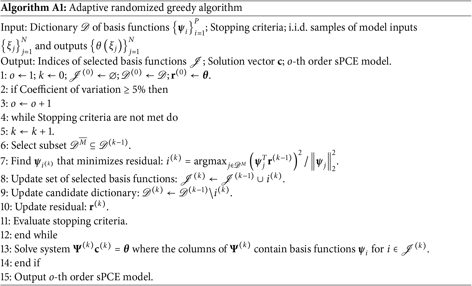
The algorithm for solving the expansion coefficients using RGA and implementing the adaptive finite-term truncation of the surrogate model via the CV is referred to as the Adaptive Randomized Greedy Algorithm (Adaptive RGA) in this paper. The algorithm’s pseudocode can be found in Appendix A. The basic steps of the algorithm are as follows:

Input Parameters: The algorithm requires a dictionary of candidate basis functions 𝒟, along with samples of input {ξj}j=1N and output {θ(ξj)}j=1N values, as well as stopping criteria.

Initialization: The algorithm starts with an order o=1, iteration k=0, an empty index set 𝒥(0)=∅, and the initial residual r(0)=θ.

Coefficient of Variation Check: If the CV of the model exceeds 5%, the model order is increased to improve accuracy.

Iteration Process: In each iteration, a subset of basis functions is selected randomly, and the best basis function that minimizes the residual is chosen using a correlation measure.

Solve System: Once the stopping criteria are met, a linear system is solved to obtain the expansion coefficients c(k), which define the model.

Output Result: The algorithm produces an accurate sPCE model.

3.2 Local and Global Sensitivity Analysis

This section performs local and global sensitivity analyses using sPCE, the global finite difference method (FDM), and Sobol’ global sensitivity index. The local sensitivity can be derived directly by taking the partial derivative of the sPCE with an objective function of θ(ξ)≈θo(ξ), where ξ=[ξ1ξ2⋯ξd]T is a d-dimensional independent random variable, and 0⩽ξα⩽1, α=1,⋯,d. The formula is as follows:

SξαsPCE=∂θ(ξ1,ξ2,⋯,ξd)∂ξαα=1,2,⋯,d(28)

The sPCE solves for sensitivity by taking a partial derivation of the polynomial, and when one of the variables takes a partial derivation, the higher-order terms of the rest of the variables will be eliminated, so that the local sensitivity can only be solved for one of the variables.

FDM, as a difference method, can perform local multivariate difference and local higher order difference compared to sPCE, because the expansion of sPCE depends on the order of the polynomial, it is not possible to solve the higher-order local sensitivity when the order is small. Sensitivity is solved with FDM dependent on the results of MCs, and traditional MCs are inefficient, so this paper combines the two methods and proposes the sPCE-FDM method to solve the sensitivity. This method uses FDM on top of the sPCE surrogate model, which ensures both accuracy and efficiency and allows for multivariate high-order sensitivity analysis.

The first and second-order sensitivities of the output of the model to the variable ξα of the sPCE-FDM are defined as follows:

Sξα(j)FDM=θ(ξα(j)+Δξα)−θ(ξα(j))Δξαα=1,2,⋯,dj=1,2,⋯,N(29)

Sξα(j)FDM=θ(ξα(j)+2Δξα)−2θ(ξα(j)+Δξα)+θ(ξα(j))(Δξα)2α=1,2,⋯,dj=1,2,⋯,N(30)

where Δξα denotes a small perturbation related to ξα. The local sensitivity of solving for two parameters with sPCE-FDM is defined as

Sξα1(j)ξα2(k)FDM=θ(ξα1(j)+Δξα1,ξα2(k)+Δξα2)−θ(ξα1(j),ξα2(k)+Δξα2)−θ(ξα1(j)+Δξα1,ξα2(k))+θ(ξα1(j),ξα2(j))Δξα1Δξα2(31)

where Δξα1 denotes a small perturbation associated with ξα1 and Δξα2 denotes a small perturbation associated with ξα2.

Global sensitivity analysis can be performed by calculating the Sobol’ global sensitivity index based on sPCE. θ(ξ) can be decomposed into the sum of 2d subfunctions.

θ(ξ)=θ0+∑α=1dθα(ξα)+⋯+θ1,2,⋯,d(ξ1,⋯,ξd)(32)

where θ0 is a constant term of order = 0 and the expectation of θ(ξ). θα(ξα) is a 1st-order subfunction of ξα, and θ1,2,⋯,d(ξ1,⋯,ξd) is an d-th order subfunction associated with all input variables. The expectation E[θ(ξ)] and variance D[θ(ξ] of the output variables are obtained directly based on the sPCE model as follows:

E[θ(ξ)]=E[∑|α|⩽ocαψα(ξ)]=a0(33)

D[θ(ξ)]=D[∑|α|⩽ocαψα(ξ)]=∑|α|⩽ocα2E[ψα2(ξ)](34)

The set of subscripts β is defined as

β=[βα,α=1,⋯,d]βα⩾0,∑α=1dβα⩽o(35)

Then the polynomial ψβ(ξ1,⋯,ξs) which contains the subscript β is

ψβ(ξ1,⋯,ξs)=∏α=1sφβα(ξα)(36)

The 0-th order orthogonal polynomial φ0(ξα) due to any variable ξα is 1. For ease of representation, define the set Ωα1,⋯,αs to contain all nonzero elements in β.

Ωα1,⋯,αs={β:βk>0,∀k∈{α1,⋯,αs}⊆{1,⋯,d};βk=0,∀k∈{1,⋯,d}∖{α1,⋯,αs}}(37)

Therefore, the orthogonal polynomials of each order of the variables (ξ1,⋯,ξs) can be expressed uniformly, and Eq. (22) can be rewritten as

θ(ξ)≈θ0+∑α=1d∑β∈Ωαcβψβ(ξα)+∑1≤α1≤α2≤d∑β∈Ωα1,α2cβψβ(ξα1,ξα2)+⋯+∑1⩽α1<⋯<αs⩽d∑β∈Ωα1,⋯,αscβψβ(ξα1,⋯ξαs)+⋯+∑β∈Ω1,⋯,dcβψβ(ξα1,⋅⋅⋅ξd)(38)

It follows from the uniqueness of the Sobol decomposition:

θα1,⋯,αs(ξα1,⋯,ξαs)=∑β∈Ωα1,⋯,αscβψβ(ξα1⋯,ξαs)(39)

It can be seen that the s-order subfunction of the variables (ξ1,⋯,ξs) in the Sobol decomposition is the sum of s-order orthogonal polynomials in the sPCE model containing the same variables. Therefore, the global sensitivity index of the input variables (ξ1,⋯,ξs) can be derived directly from sPCE.

Sα1⋯αsSobol=∑β∈Ωα1,⋯,αscβ2E[ψβ2(ξα1,⋯,ξαs)]∑|α|⩽ocα2E[ψα2(ξ)](40)

The explicit expressions for the surrogate model of structural dynamics can be derived using the MPM and sPCE methods according to the above description. The local sensitivity of the model to a particular variable can be obtained by differentiation, the local sensitivity of the model to multiple variables can be obtained by sPCE-FDM, and the global sensitivity of the model can be analyzed by the Sobol method. Fig. 2 illustrates a sketch of the sensitivity-solving process based on sPCE.

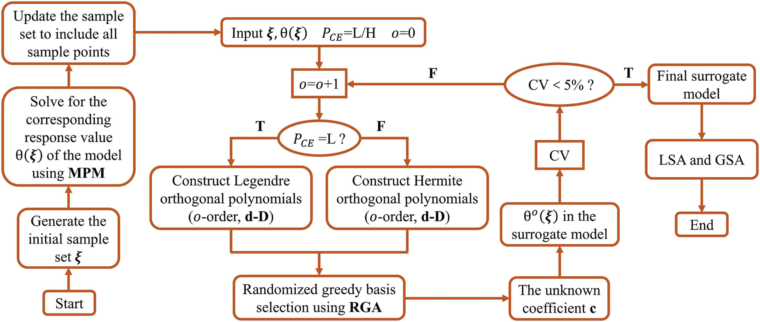
Figure 2: A sketch of the computational flow for constructing sPCE surrogate models for sensitivity analysis using the adaptive randomized greedy algorithm

4  Numerical Examples

In this section, physical models for collision, vibration, and penetration deformation in structural dynamics are constructed using MPM, and various response surface models are developed as surrogate models for MPM. The effectiveness of the proposed adaptive RGA and sPCE-based sensitivity analysis methods in structural dynamics is highlighted through comparisons. In the collision deformation analysis (Section 4.1), the training data follows a normal distribution, and the accuracy and efficiency of the response surface models are compared under different numbers of training samples, verifying the correctness of sPCE and FDM in solving local sensitivities. In the vibration deformation analysis (Section 4.2), the training data follows a uniform distribution, and the local and global sensitivities of sPCE-FDM are compared at different orders. In the penetration deformation analysis (Section 4.3), the training data set does not follow any specific distribution. Therefore, the Legendre and Hermite polynomials of sPCE are established, and the accuracy, result variability, and Sobol indices of the two sPCE models are compared using the same training data set.

The framework for MPM and the adaptive sPCE method are implemented in MATLAB and executed on a personal computer equipped with an Intel (R) Core (TM) i7-7700 CPU and 128 GB of RAM.

4.1 Collision Deformation Analysis

Collision deformation refers to the deformation that occurs in materials and structures when subjected to rapid impacts, a phenomenon widely observed in fields such as bearing systems and automotive collisions. During a collision, the object experiences a significant force over a very short time, leading to substantial changes in its shape, structure, and internal stress state. Depending on the nature and magnitude of the impact, collision deformation can manifest as elastic collisions, plastic deformation, or material rupture and damage. This section first examines the elastic collisions between the balls in bearing systems, as illustrated in Fig. 3. Although the contact area is small, the rolling balls continuously undergo microelastic collisions during high-speed operation, which, to some extent, affect the bearing’s lifespan and efficiency.

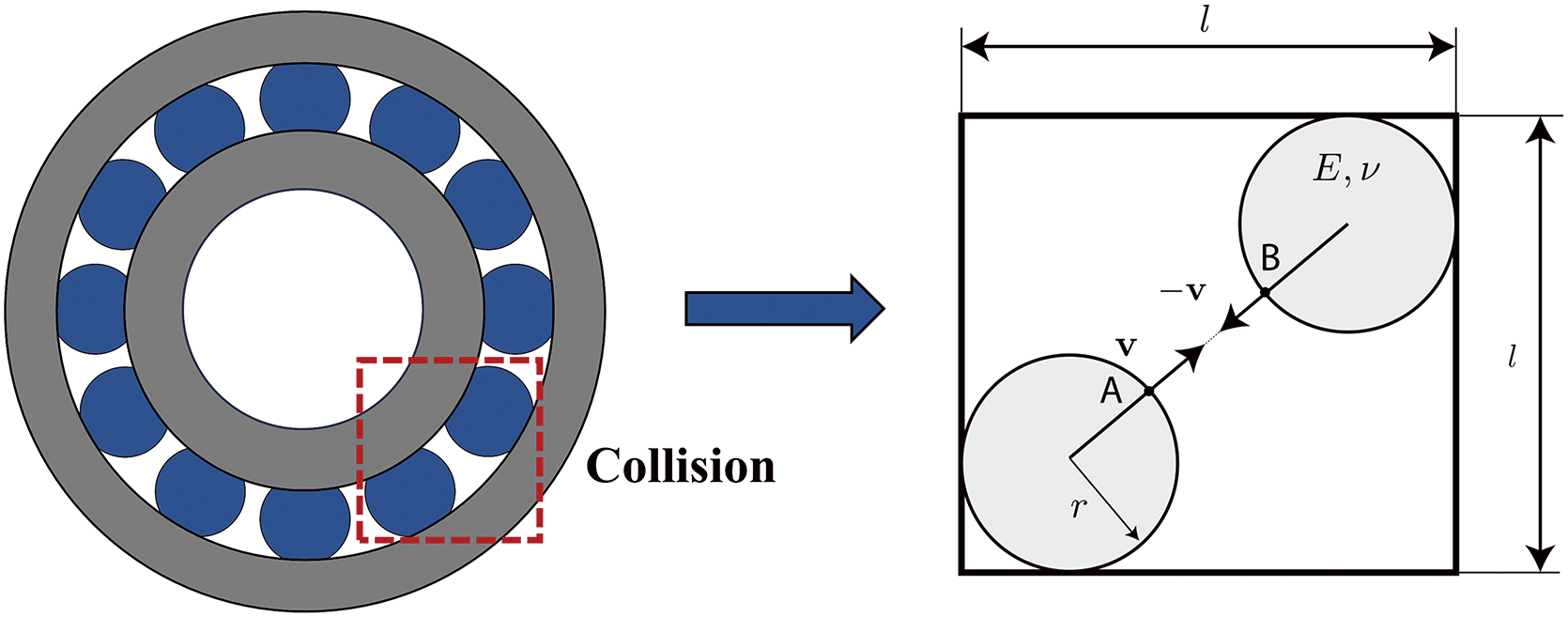
Figure 3: The schematic diagram of ball collisions in a bearing system

Based on the collision problem proposed by Sulsky et al. [5], an MPM model for elastic collisions between balls is established. It is assumed that there are no boundary conditions or external forces involved. Before the collision, the two balls are in a rigid body motion state, with both stress and strain being zero. The physical model is solved using the CPDI-Q4 formulation.

The collision process is captured in a physically realistic manner, where kinetic energy is reduced during impact and subsequently recovered mainly after separation. The strain energy attains its peak magnitude at the juncture of maximum deformation during the impact event, subsequently diminishing to a level corresponding to the free vibration state of the ball. The parameter settings of the physical model are shown in Table 1. The motion and stress state of the two balls are depicted in Fig. 4.

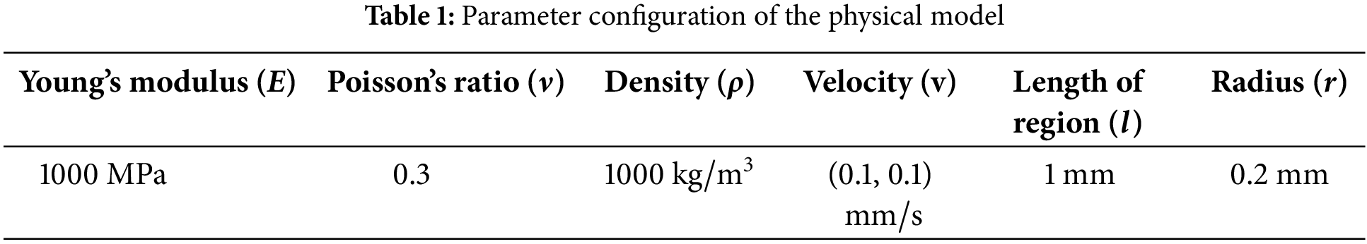
Figure 4: Elastic collision of balls in bearing systems: snapshots and stress states at different times (T = 0, 1, 1.5, 2 s)

The physical model established by MPM is usually ideal, so it is necessary to consider uncertainty factors of the real situation, which include material properties, external loads, and so on. In this example, the sPCE surrogate model is constructed using the adaptive randomized greedy algorithm with Young’s modulus and density as input variables and the strain energy as output variable.

As shown in Fig. 5, the uncertainty ranges for Young’s modulus (E) and density (ρ) are set to a mean value of 1000 and a standard deviation of 100, random sampling are performed in the range from Nθ=100 to Nθ=500. Hermite polynomials are chosen for the orthogonal polynomials, and the dataset [ξ, θ(ξ)] obeys a Gaussian distribution, so as to simulate the effects of the differences in material properties on the model.

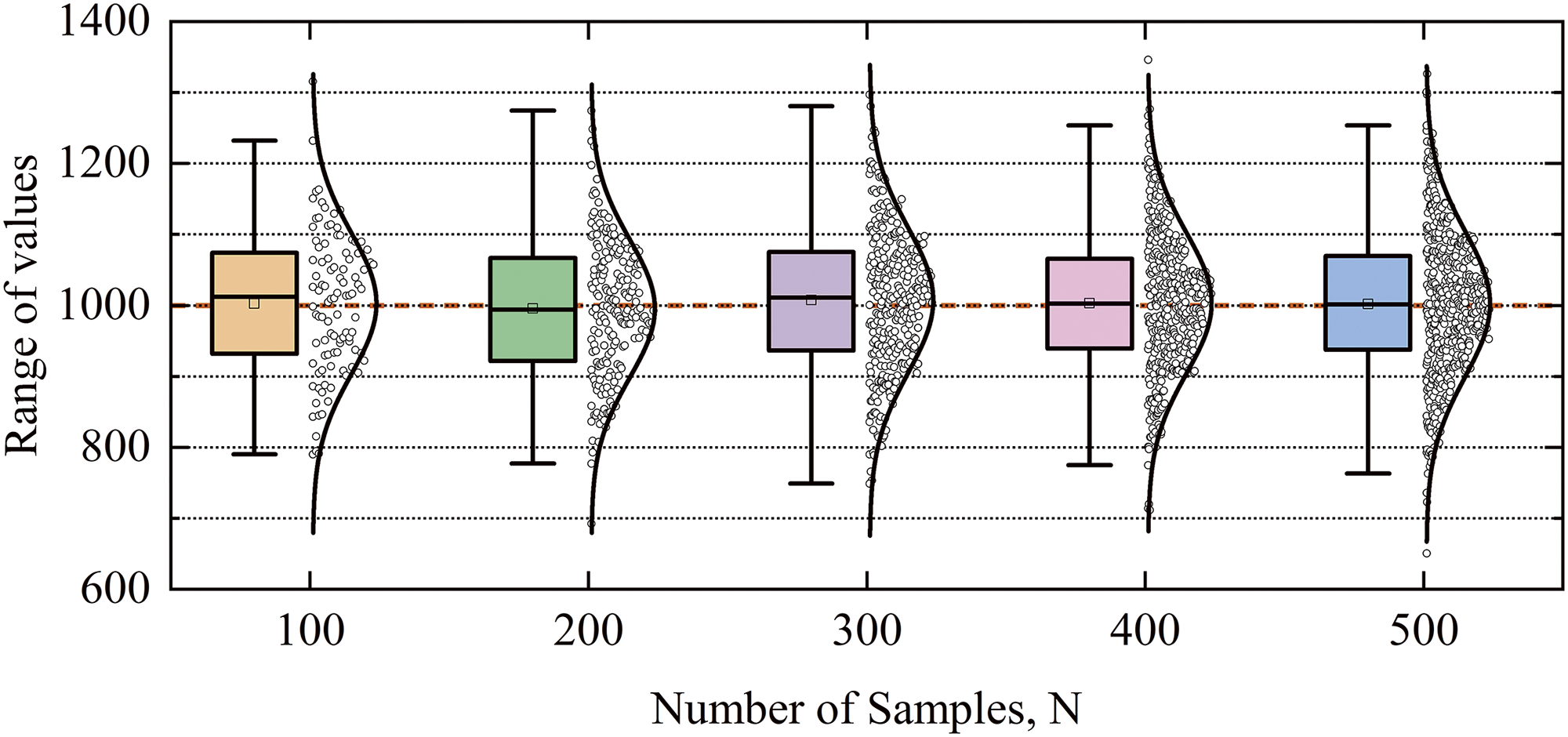
Figure 5: Random sampling at different sample sizes from Nθ=100 to Nθ=500 where the dataset follows a Gaussian distribution

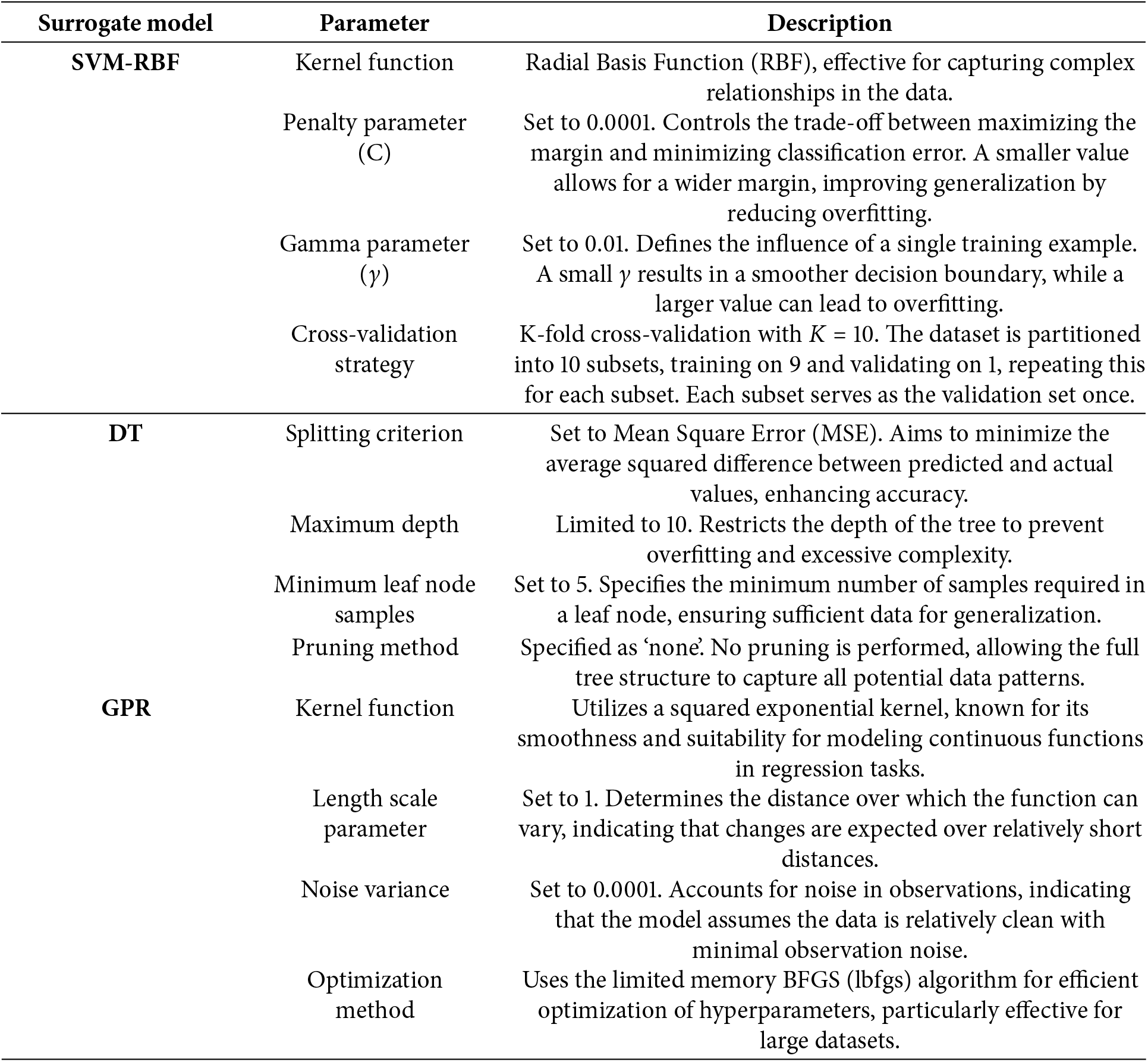
To verify the feasibility of the response surface model as a surrogate model for MPM, as well as the accuracy and efficiency of constructing sPCE using adaptive RGA, surrogate models for the structural dynamics problem were constructed using a support vector machine with radial basis function chosen for the kernel function (SVM-RBF), gaussian process regression (GPR), and decision tree (DT) with the same training samples. The reason for choosing the above algorithms to construct the response surface models is that they perform excellently in handling nonlinear relationships and high-dimensional data, effectively capturing complex input-output mappings. The parameter configuration of each algorithm is shown in Appendix B.

The metrics for comparison include the mean relative error (MRE) and the relative standard deviation (RSD) that approximate the statistics, and their formulas are as follows:

MRE=1N∑j=1N|θo(ξ(j))−θ(ξ(j))|θ(ξ(j))(41)

RSD=∑j=1N[θo(ξ(j))−θ¯(ξ)]2N−1/θ¯(ξ)(42)

As shown in Fig. 5, with the increase of the number of training samples, the MRE and RSD of the surrogate models obtained by the four algorithms show a decreasing trend. Among them, the relative error of SVM-RBF is larger, indicating that the accuracy of the surrogate model is worse compared with other algorithms. In contrast, the mean error of adaptive RGA has been at a low level, and the standard deviation reaches a low level when the number of training samples reaches 300 or more and has maintained the highest accuracy.

Fig. 6 shows the performance of different models (SVM-RBF, GPR, DT, and Adaptive RGA) under varying sample sizes. The results indicate that as the sample size increases, the MRE and RSD of all models decrease, suggesting that a larger sample size improves the accuracy and stability of the models. Among all sample sizes, Adaptive RGA consistently exhibits the lowest MRE and RSD, especially when the sample size is small (e.g., N = 100), demonstrating superior accuracy and stability compared to the other models. In contrast, SVM-RBF shows larger errors and more fluctuations when the sample size is small, indicating its sensitivity to sample size. Overall, Adaptive RGA shows a significant advantage in handling small sample problems, and it maintains good accuracy and stability even with larger sample sizes, making it suitable for high-precision structural dynamic analysis.

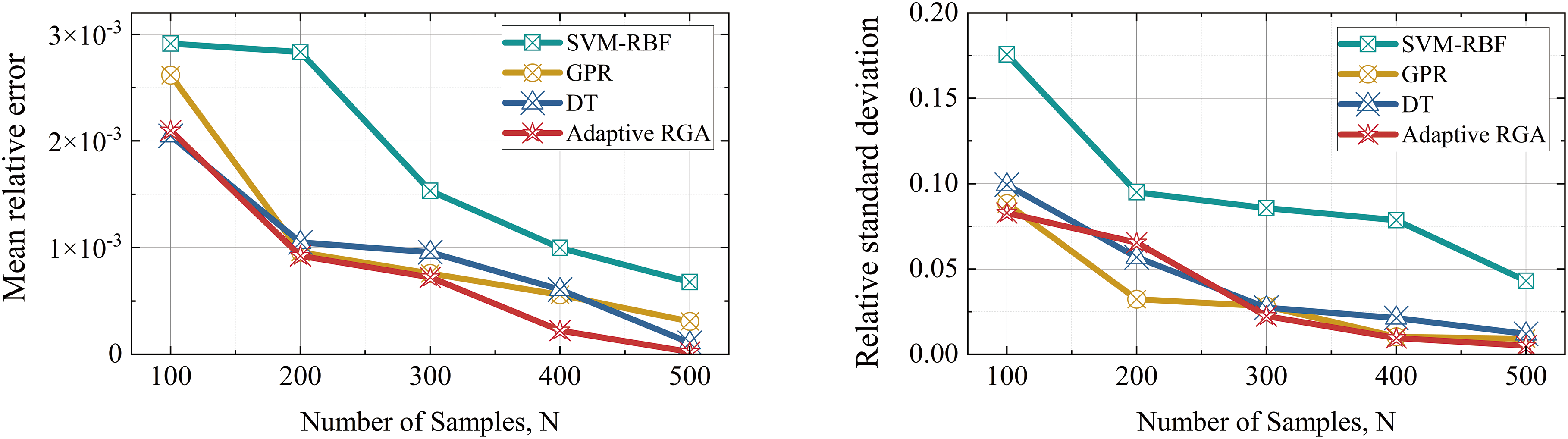
Figure 6: Comparison of relative errors of mean (left) and standard deviation (right)

In addition to accuracy, efficiency is another crucial factor for the suggested strategy. The time cost function in MPM can be explicitly specified as

TMPM(N~)=N~×tMPM(43)

which relies on the number of sampling points, the time tMPM is the time of a single MPM calculation. The time cost of the general surrogate model and the sPCE surrogate model are defined as

Tsurmod(Nθ,Nθo)=tsurmod,train(Nθ)+tsurmod,eval(Nθo)(44)

TsPCE(Nθ,Nθo,o,d)=tsPCE,train(Nθ,o,d)+tsPCE,eval(Nθo)(45)

which relies on the training time tsPCE,train and the predicting time tSPCE,eval with Nθo=N~.

As shown in Fig. 7, the left figure shows the variation in runtime with increasing sample size for five methods (MPM, SVM-RBF, GPR, DT, and Adaptive RGA), while the right figure compares the runtime trends of different orders of the sPCE model as sample size increases. In the left figure, the running time of the MPM method is significantly higher than the other methods and increases rapidly as the sample size grows. When calculating the same 500 samples, the computational efficiency of using a response surface model as a surrogate model is improved by about 83% compared to MPM. Among them, the running time of the Adaptive RGA remains the lowest, demonstrating its significant advantage in computational efficiency. The right figure indicates that as the order increases, the runtime of the sPCE model slightly increases, but the overall growth is slow, suggesting that the time complexity of the sPCE method is relatively stable across different orders.

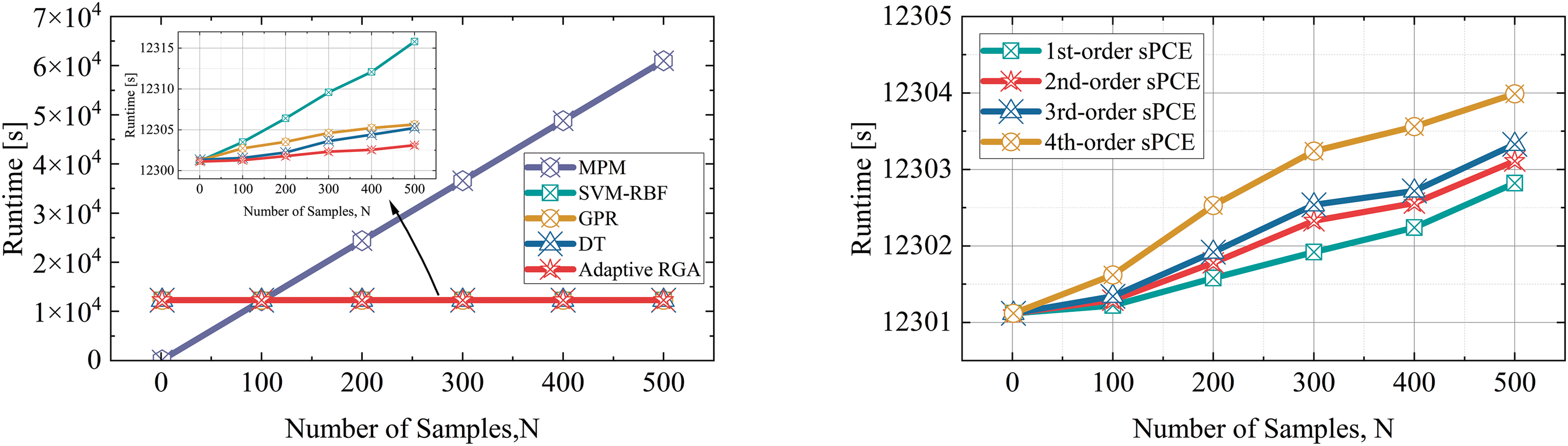
Figure 7: Comparison of runtimes with different sample sizes: physical model and different surrogate models (left), sPCE surrogate model with different orders (right)

Table 2 demonstrates the regression evaluation metrics for the different surrogate models, including mean (μ), standard deviation (σ), coefficient of variation (CV) and coefficient of determination (R2), and the tests are performed with a training sample size of 500. The adaptive RGA is truncated at o=2, resulting in a 2nd-order sPCE model. In comparison, the SVM-RBF model exhibits the highest relative variability and the lowest R2, indicating that its reliability for this application may be relatively low. Models such as GPR and DT demonstrate reasonable accuracy and stability, making them viable alternatives. In conclusion, sPCE allows customization of the order, providing greater flexibility, making it an effective alternative modeling method for accurately capturing the structural dynamics of the MPM.

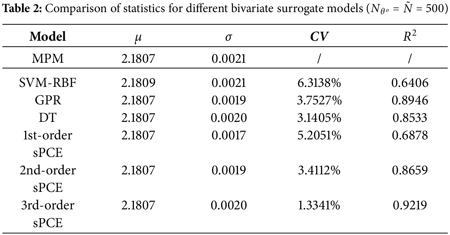
Table 3 shows the parameter configurations and local sensitivity results for the sPCE surrogate model. It can be seen that the local sensitivities obtained by both the sPCE method and the FDM method are in a low range, where Young’s modulus is more sensitive than the density, which has a greater impact on the results. As shown in Fig. 8, the local sensitivity first decreases and then tends to stabilize with the increase of Young’s modulus, the local sensitivity decreases slowly and then tends to decrease more as the density increases. It is shown that the use of adaptive RGA to construct the sPCE surrogate model for local sensitivity analysis is effective.

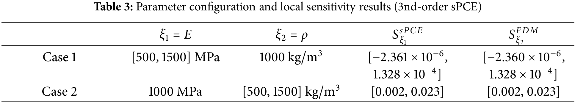
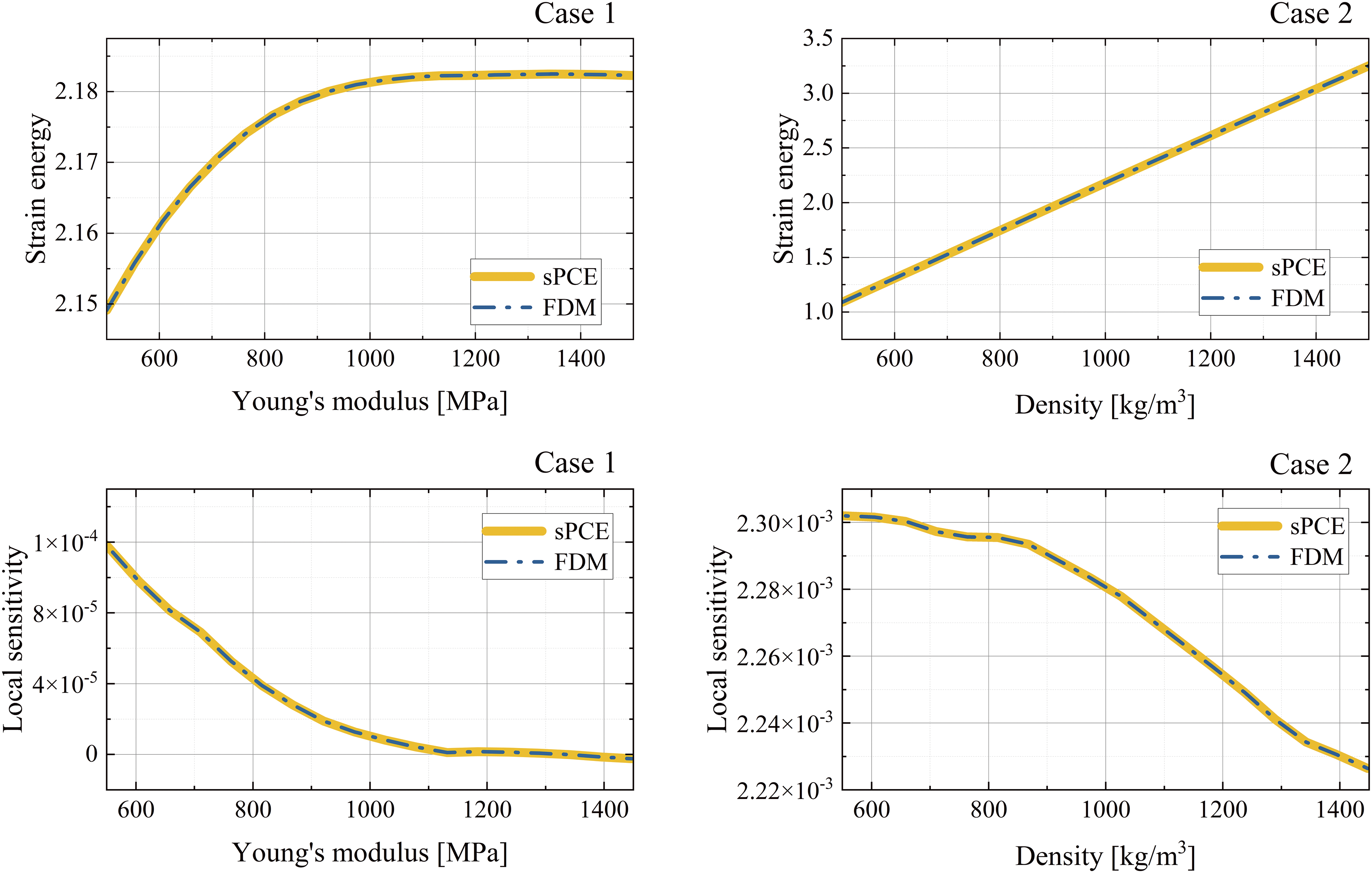
Figure 8: Comparison of local sensitivity between sPCE (d=2, o=3) and FDM

To discuss how the adaptive RGA scales in constructing the sPCE surrogate model with increasing structural system complexity, an MPM physical model of car collision deformation was established. Compared to the ball collision problem in the bearing system, the structure of a car is more complex, with 67,300 material points discretized. The material point model and stress states at different time steps are shown in Fig. 9, with material properties provided in Table 1.

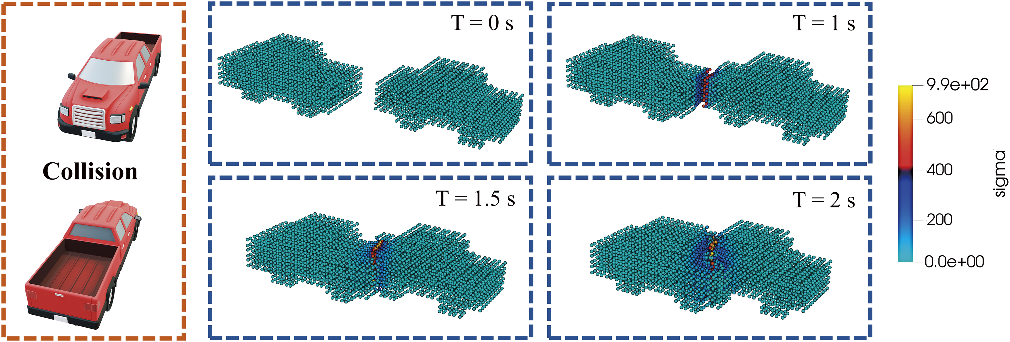
Figure 9: MPM modeling of automobile collisions and the stress state at different moments

MCs were used to randomly sample within the uncertainty range, with the uncertainty ranges for Young’s modulus and density set as a mean of 1000 and a standard deviation of 100. The sampling was conducted with 1000 and 200 samples, respectively. The results from the 1000 samples, calculated through MPM, serve as the benchmark for comparing the accuracy of the other three algorithms. The 200 samples, calculated through MPM, are used as training data for the SVM-RBF, GPR, DT, and sPCE models. For the sPCE model, Legendre polynomials were selected for the orthogonal polynomial, and truncation was performed at o=5 using the adaptive RGA.

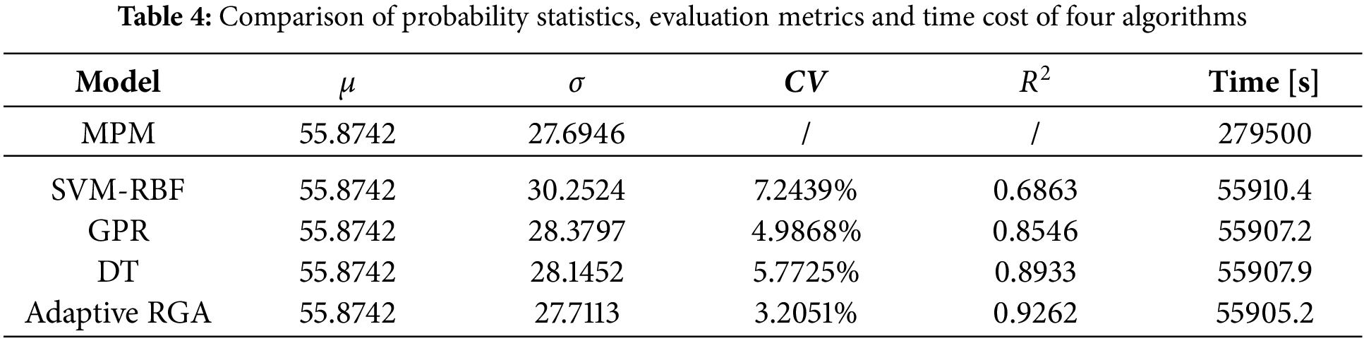
Table 4 presents a comparison of probability statistics, evaluation metrics, and time cost between four algorithms and the MPM method. In comparison, the four algorithms (SVM-RBF, GPR, DT, and Adaptive RGA) maintain consistency in terms of the mean, while Adaptive RGA has a standard deviation closest to that of MPM, the lowest CV (3.2051%), and the highest R2 (0.9262). This indicates that Adaptive RGA outperforms the other algorithms in terms of accuracy and stability. In addition, compared to the MPM method, the four surrogate modeling algorithms improved efficiency by about 80% when calculating 1000 datasets. Among them, the sPCE surrogate model constructed by the adaptive RGA achieved the shortest computation time, demonstrating outstanding computational efficiency and accuracy.

4.2 Vibration Deformation Analysis

In the process of bridge construction [41,42], the vibrational deformation of cantilever beams is one of the key factors affecting structural performance and construction safety. During the construction phase, cantilever beams bear loads and environmental influences that change continuously, causing complex vibrational and deformation responses in both vertical and horizontal directions. These vibrational deformations not only reduce construction accuracy, leading to the accumulation of deviations, but also have the potential to trigger structural stability issues, increase fatigue stress, and negatively affect the long-term safety of the bridge. Therefore, this chapter primarily analyzes the vibrational deformation of cantilever beams during bridge construction, as shown in Fig. 10.

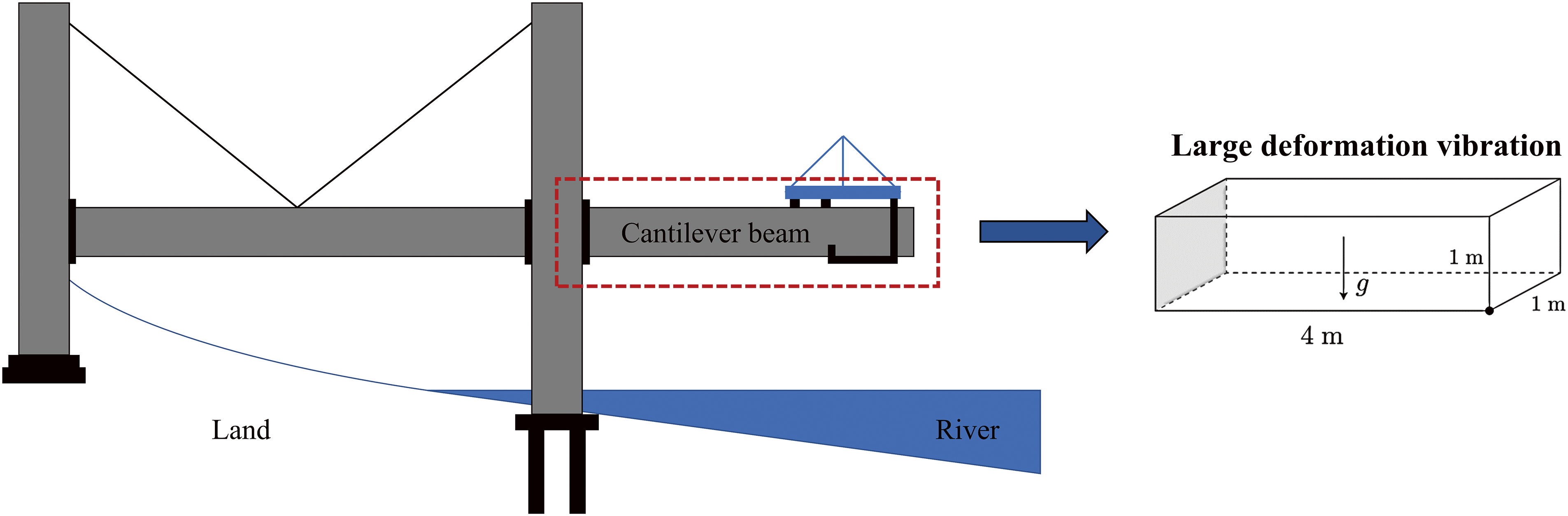
Figure 10: Schematic diagram of the vibration deformation of the cantilever beam during bridge construction

The deformation vibration model of a flexible cantilever beam during the bridge construction process was developed using MPM with reference to the framework proposed by Sadeghirad et al. [43]. The cantilever beam is characterized by its softness and substantial gravitational load. The cantilver beam is made of a hyperelastic material, which is modeled by a Neo-Hookean constitutive model. The parameter settings of the physical model are shown in Table 5. The background grid consists of 8 × 8 × 2 cells. The physical model was solved using the CPDI-Tet4 formulation. Fig. 11 illustrates the time snapshots and the stress states in the X and Y directions.

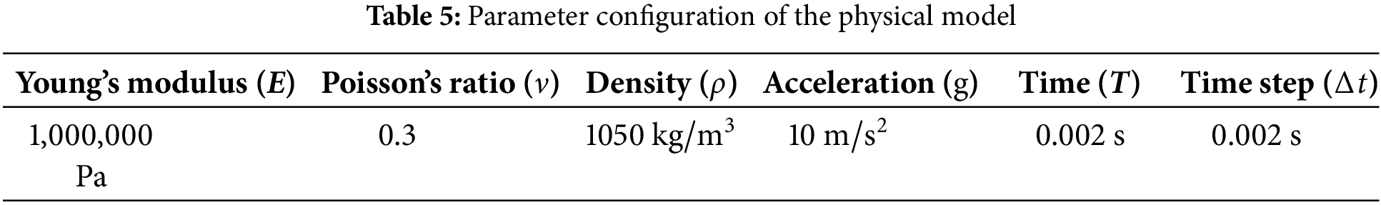
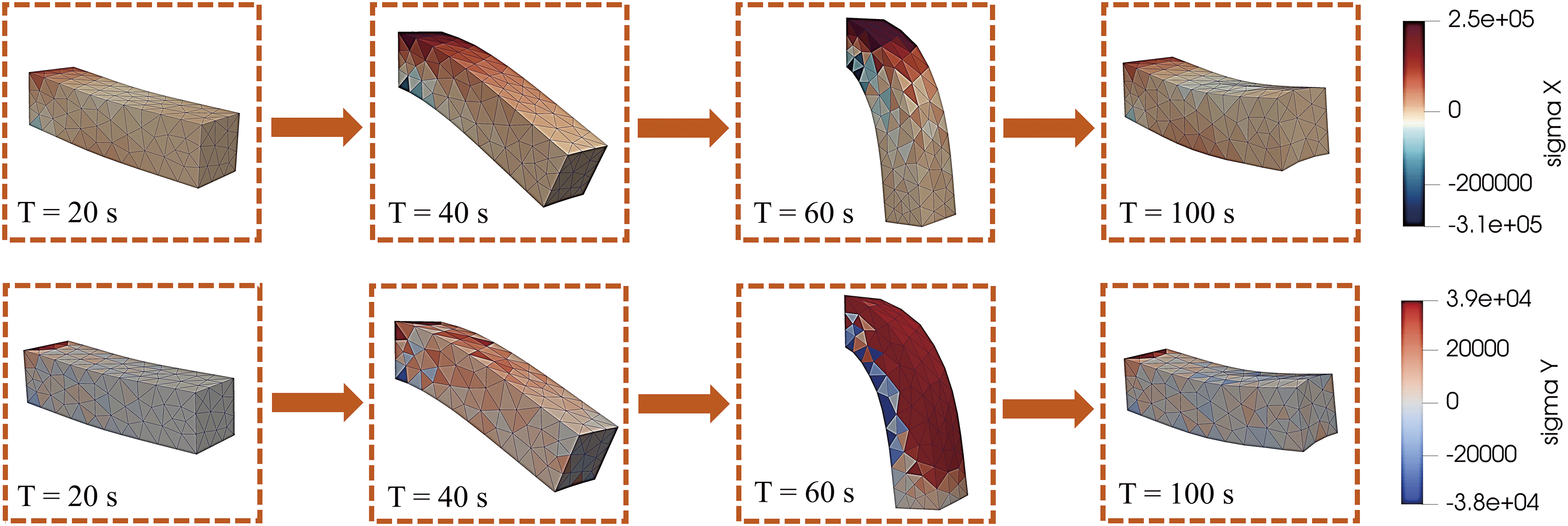
Figure 11: The snapshots in time of the physical model and the stress state in the X and Y directions

In this example, the study considers both external and internal factors on the output. An adaptive RGA was used to construct the sPCE surrogate model with acceleration (g) and Young’s modulus (E) as input variables and displacement as output variables. The uncertainty range of acceleration is set to [0, 50] and that of Young’s modulus is set to [800000, 1200000]. Sequential sampling is performed within the range. Legendre polynomials are chosen for the orthogonal polynomials and the dataset is a 2D dataset obeying a uniform distribution.

The SVM-RBF, DT, GPR, and sPCE surrogate models were trained using 200 uniformly distributed samples. As shown in Table 6, the predicted mean values across models are mostly around −3.5710, with a slight deviation in the SVM-RBF results. DT and higher-order sPCE models exhibit larger standard deviations, indicating a broader variable range to capture system responses. The adaptive RGA terminates at o=3 with (CV = 4.3216%) and (R2 = 0.9396), suggesting good convergence and prediction performance for the 3rd-order sPCE model. The (CV > 5%) in SVM-RBF and GPR reflects larger prediction errors and limited generalization, while DT, with a low CV and R2 near 1, shows strong data fit.

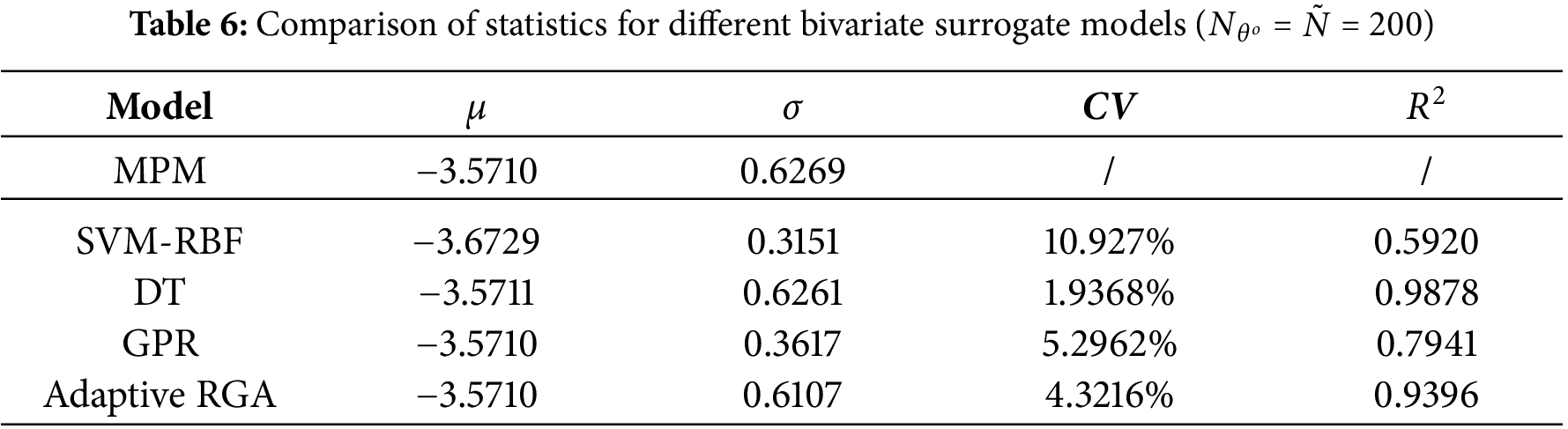
Fig. 12 illustrates the comparison of the sPCE surrogate model with the MPM results, as well as the comparison of the relative errors of different orders. It can be seen that the 3rd-order sPCE surrogate obtained by the adaptive randomized greedy algorithm has higher accuracy, but the 5th-order sPCE is closer to the physical model constructed by the material point method. The relative error is calculated as RE=|θo(ξ(j))−θ(ξ(j))|/θ(ξ(j)). The comparison of relative errors by different orders shows that an increase in the order leads to a decrease in the model error and thus to a higher accuracy. In 5th-order sPCE, the model error increases as the value of g decreases, while a higher value of g mitigates the error fluctuations. The peaks at g=19.8961 m/s2 and E=1,086,460Pa indicate that the model is unstable in this parameter space.

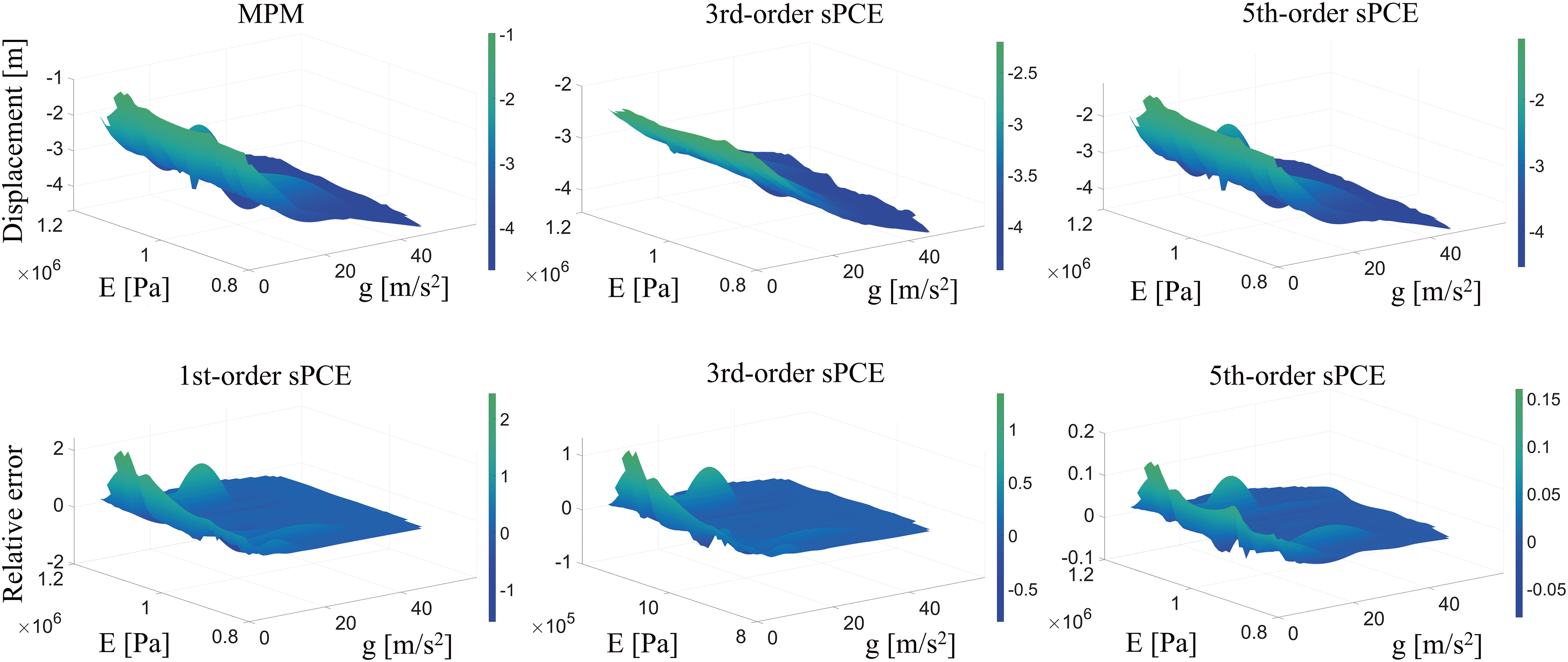
Figure 12: Comparison of sPCE surrogate model with MPM results (top), and comparison of normalized errors of different orders (bottom)

The four cases and parameter configurations for local and global sensitivity analyses are given in Table 7. As can be seen in Fig. 13, the 3rd-order sPCE constructed by the adaptive RGA can accurately demonstrate the local sensitivity and match the sensitivity results of higher-order sPCE. In Case 1, the local sensitivity first decreases with increasing Young’s modulus, minimizes at E=982,462 Pa, and then increases. In Case 2, the local sensitivity first increases with increasing acceleration maximizes at g=29.3 m/s2, and then decreases.

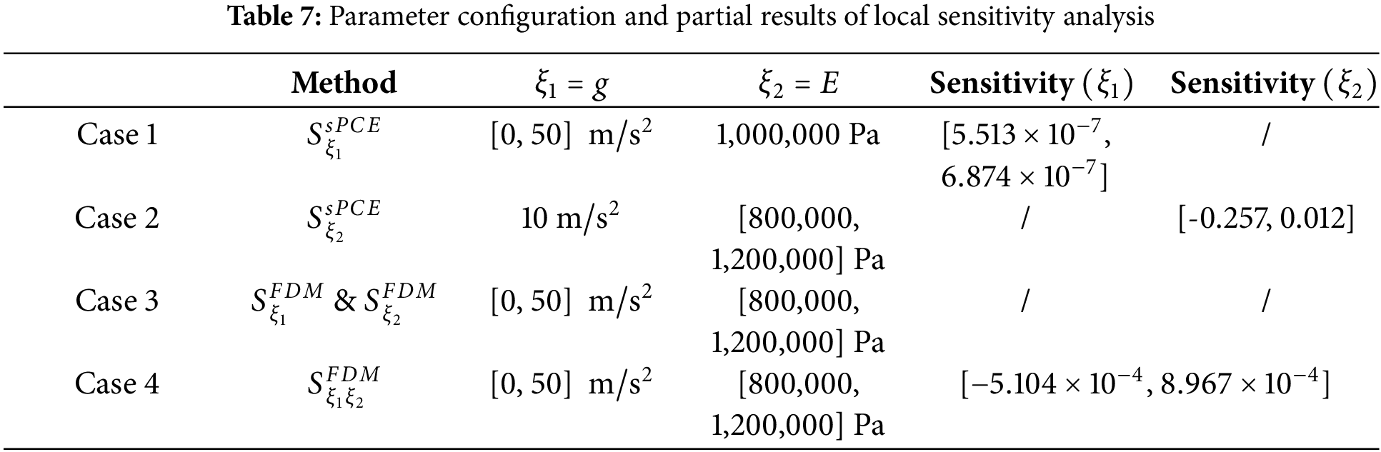
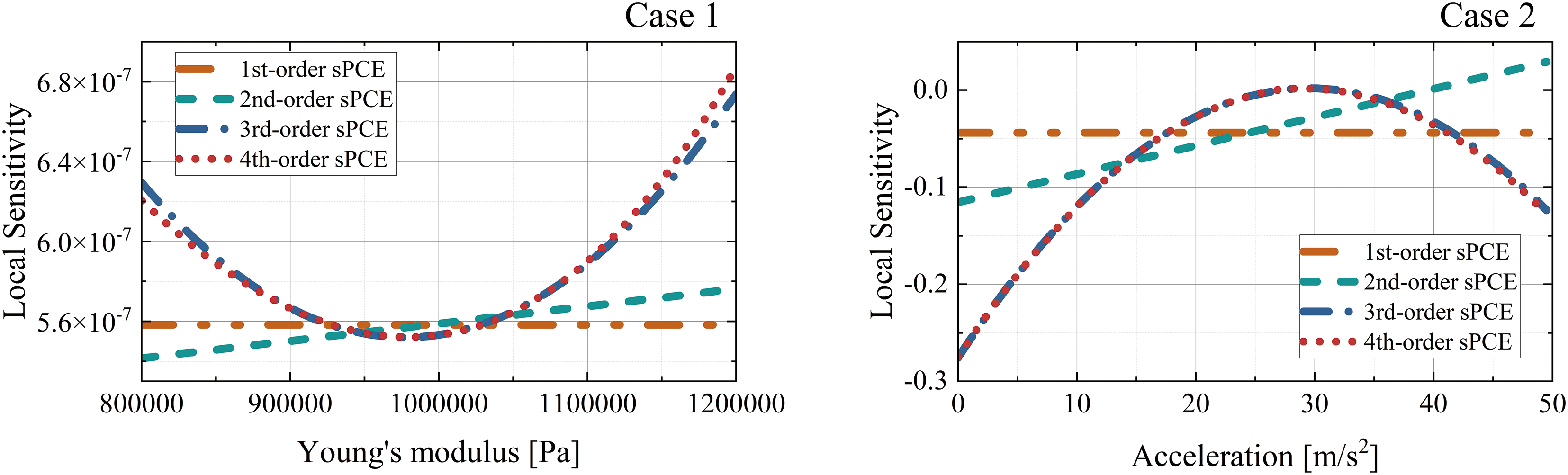
Figure 13: Comparison of local sensitivities for different orders of sPCE

In Case 3, the first-order second-order, and third-order sensitivities of the model are solved separately by sPCE-FDM, as shown in Fig. 14. The first-order local sensitivity of the model tends to decrease with increasing acceleration g by introducing small perturbations to the input parameter g while keeping E constant, indicating a reduced effect on the output. The second-order local sensitivity changes from large to small as g increases and fluctuates in the interval [10, 40] with a consequent increase in sensitivity. The third-order local sensitivity is initially small in the interval [0, 17] and fluctuates with a gradual increase in g. The magnitude of the fluctuations increases. Thus, the model output is highly sensitive to higher-order terms.

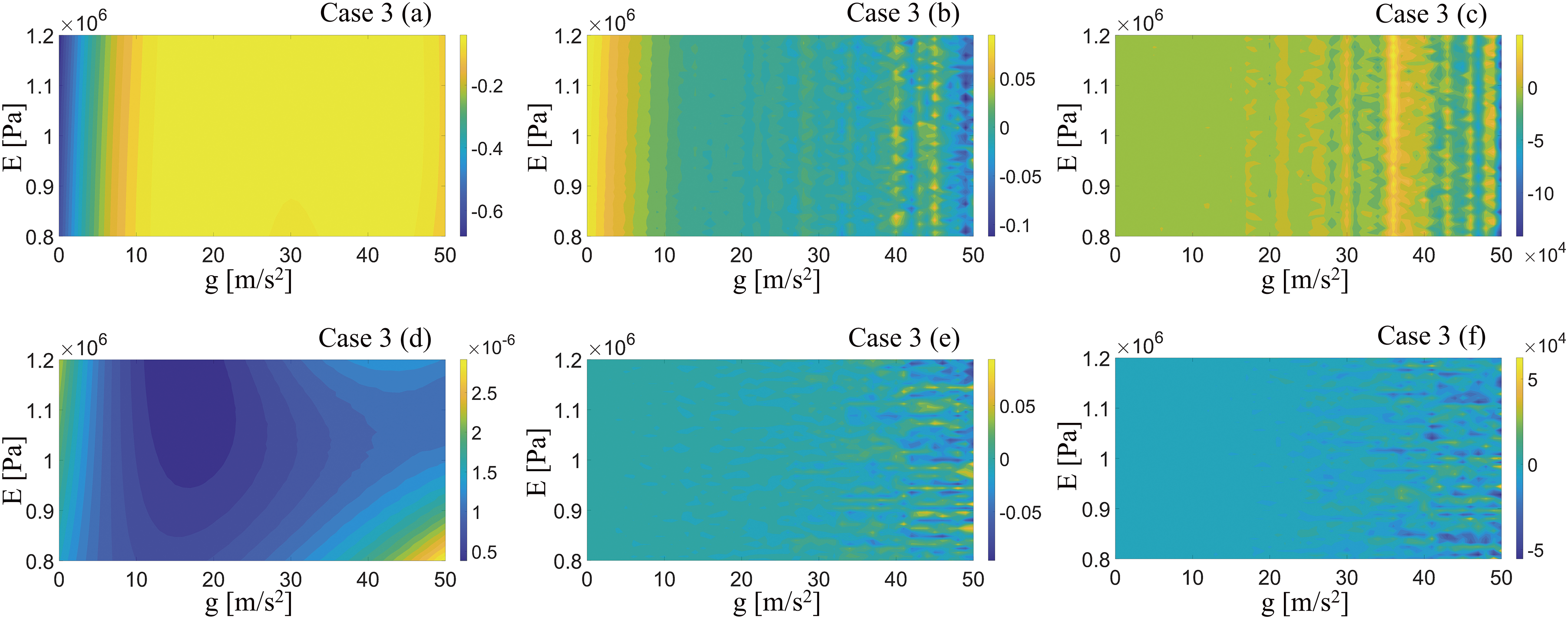
Figure 14: (a–c) represent the first-order, second-order and third-order local sensitivities of acceleration, (d–f) represent the first-order, second-order and third-order local sensitivities of Young’s modulus

The first-order local sensitivity of the model does not show a significant trend as the parameter E increases with a small perturbation of the input parameter E while the parameter g is kept constant, indicating that the change in the parameter E does not have a significant effect on the output. The second-order local sensitivity remains consistently small as E increases, but the sensitivity begins to fluctuate at g>30 m/s2, suggesting that the parameter E has a small effect on the model sensitivity, and conversely, the effect of the parameter E on the model sensitivity is closely related to the parameter g. The third-order local sensitivity, which is similar to the second-order local sensitivity, remains small as E increases. It is always affected by g, indicating that the model output is insensitive to higher-order terms in E.

In Case 4, the local sensitivity analysis using sPCE-FDM shows how the system output responds to simultaneous changes in two input parameters. Fig. 15 shows that simultaneous tuning of the input parameters g and E increases the sensitivity of the model. The sensitivity peaks between g=50 m/s2 and E=1,150,000 Pa, indicating high volatility. The sensitivity of the model is slightly affected by the E correction. A comparison of the 1st-order sPCE, 3rd-order sPCE, and 5th-order sPCE models shows that the curvature of the surrogate model increases with the increase of the model order, which is conducive to a better simulation of the steep regions in the original model. FDM on sPCE above the third order allows a better representation of sensitivity information and raw data.

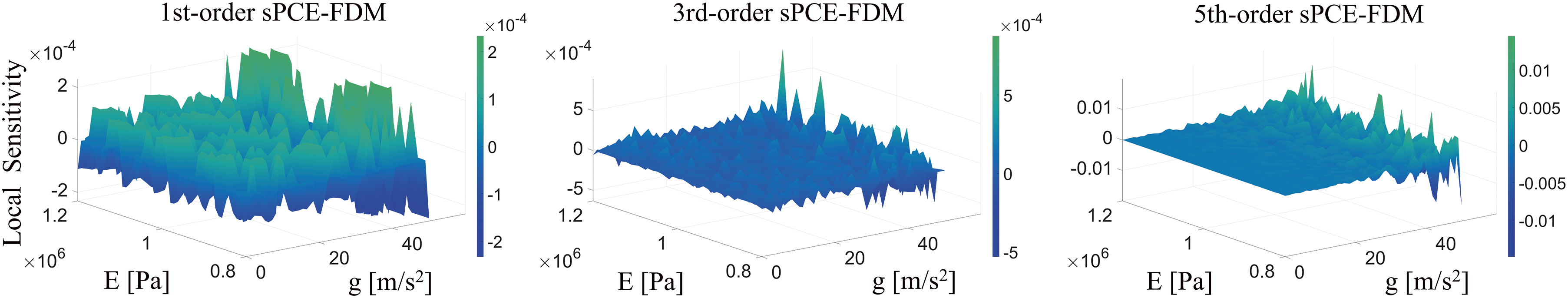
Figure 15: Comparison of sPCE-FDM local sensitivity for bivariate surrogate models of different orders

Finally, the Sobel index was calculated on the basis of the 3rd-sPCE surrogate model, where S1 stands for the first-order Sobol effect index, and ST stands for the Sobol total effect index. The global sensitivities where the input variable is Young’s modulus are S1 = 0.01926 and ST = 0.01733, the global sensitivities of the acceleration are S1 = 0.97136 and ST = 0.97694 The analysis of the first-order Sobol index and total Sobol index for the different variables shows that the change in Young’s modulus has less effect on the model output and the change in acceleration has more effect on the model output.

4.3 Penetration Deformation Analysis

In the military field, protective structures such as Hardened Aircraft Shelter (HAS) are often exposed to the threat of high-speed penetration weapons such as ballistic missiles and armor-piercing bullets. To evaluate the structural deformation and impact resistance of the bunker when subjected to penetration attack, it is of great significance to analyze its penetration deformation in depth. In this paper, the aircraft shelter structure is selected as the research object, as shown in Fig. 16.

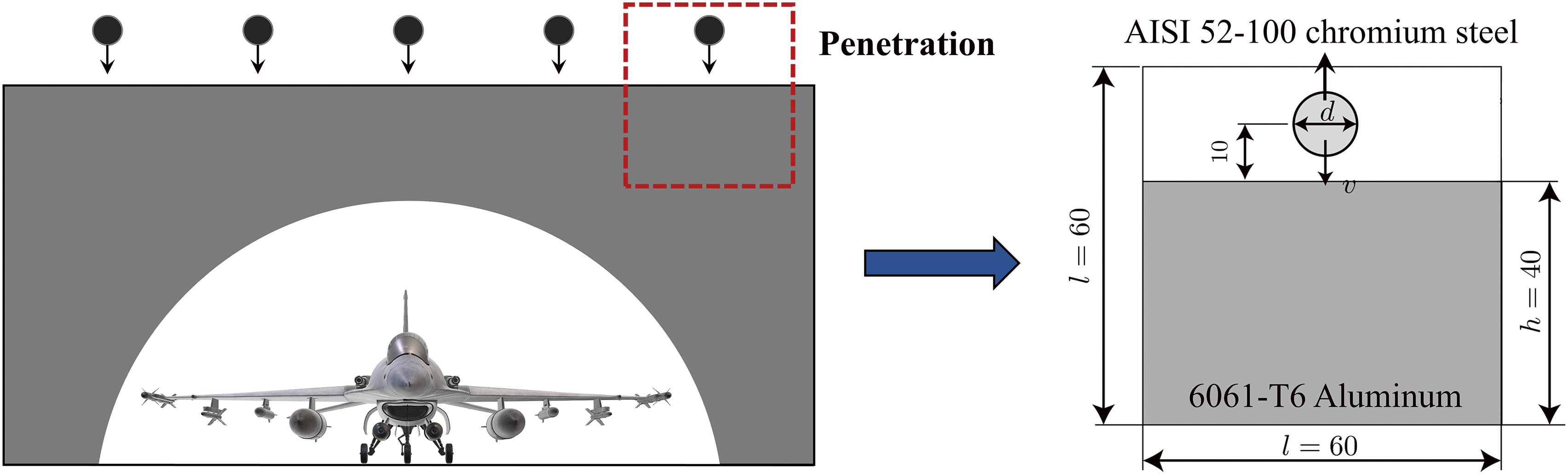
Figure 16: Schematic diagram for penetration analysis of HAS

The theoretical model of HAS was established with the shelter made of 6061-T6 aluminum and the missile made of AISI 52-100 chrome steel. The modeling of penetration was developed concerning the problem posed by Sulsky et al. [44] and later explored by Coetzee [45] and inspired by experiments performed by Trucano et al. [46]. The steel ball is presumed to be linearly elastic, while the aluminum target follows an elastically perfect plastic behavior as per the von Mises yield criterion. The boundary represents the computational domain (50 × 50 elements). There are 6700 particles for the aluminum target and 204 particles for the steel ball. The parameter configurations of the physical model are shown in Table 8. Motion and von Mises stress distributions are illustrated in Fig. 17. Notably, the steel ball exhibits no deformation, consistent with the findings of Trucano and Grady. The depth of penetration aligns well with MPM results reported by Coetzee.

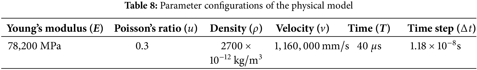
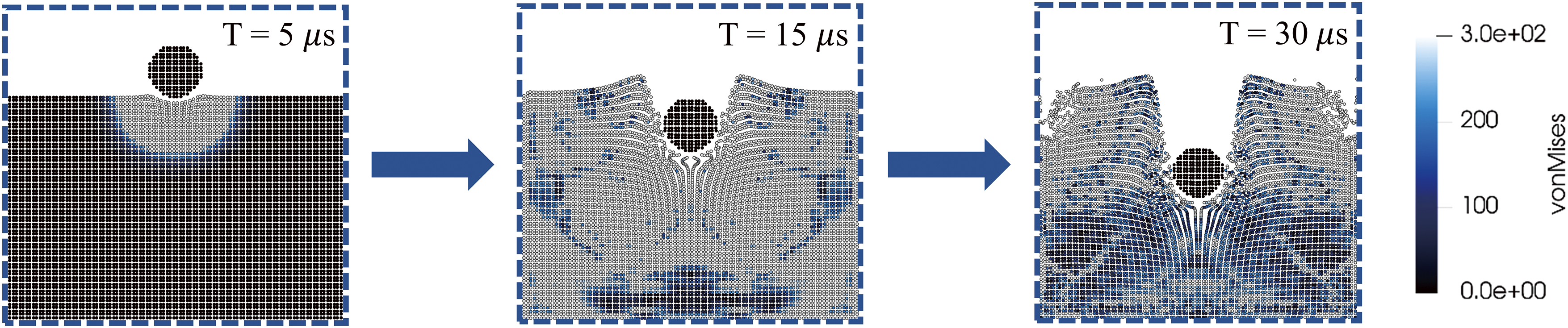
Figure 17: The process of penetration of a localized region of the HAS: von Mises stress distribution at different time points

In this example, the sPCE surrogate model was constructed using an adaptive RGA with Young’s modulus (E), Poisson’s ratio (u), and velocity (v) as input variables and strain energy as output variables. As shown in Fig. 18, the variation range of Young’s modulus is [75,000, 80,000], Poisson’s ratio is [0.25, 0.35], and the variation range of density is [1,100,000, 1,200,000]. Random samples are taken within the variability range and the sampling results do for testing the variability of choosing different orthogonal polynomials for constructing the sPCE surrogate model under the same training dataset.

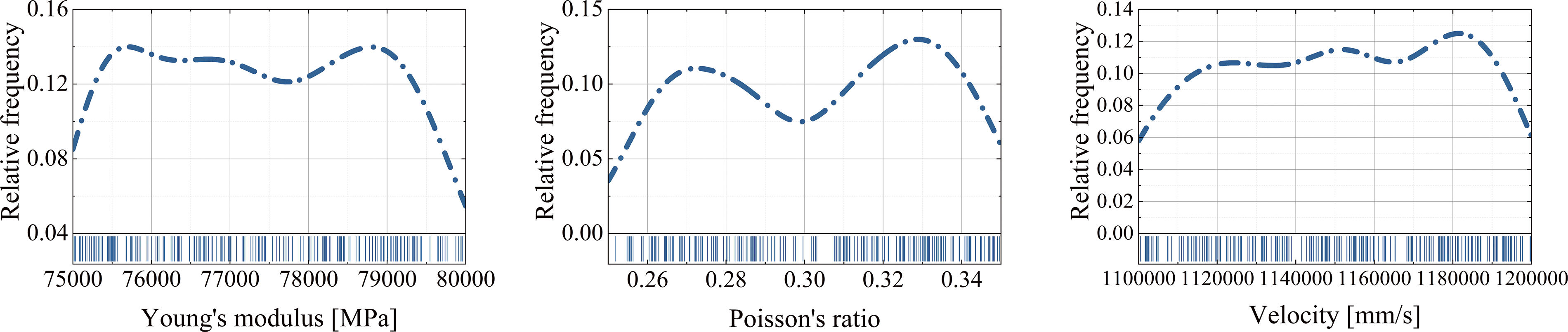
Figure 18: Random sampling ranges for the three variables

As can be seen in Table 9 that the differences in several statistics of sPCE obtained by choosing different orthogonal polynomials are small under a randomly sampled training dataset. The μ values of the prediction results are the same under different orders, and the σ of the sPCE constructed by the Legendre polynomial is overall higher than that of the sPCE constructed by the Hermite polynomial. Both have good fit and prediction performance at lower orders by comparison of CV and R2. It is verified that the variability of the sPCE surrogate models constructed by choosing two different orthogonal polynomials is less as well as the accuracy of the models is guaranteed under a training dataset that does not obey any distribution.

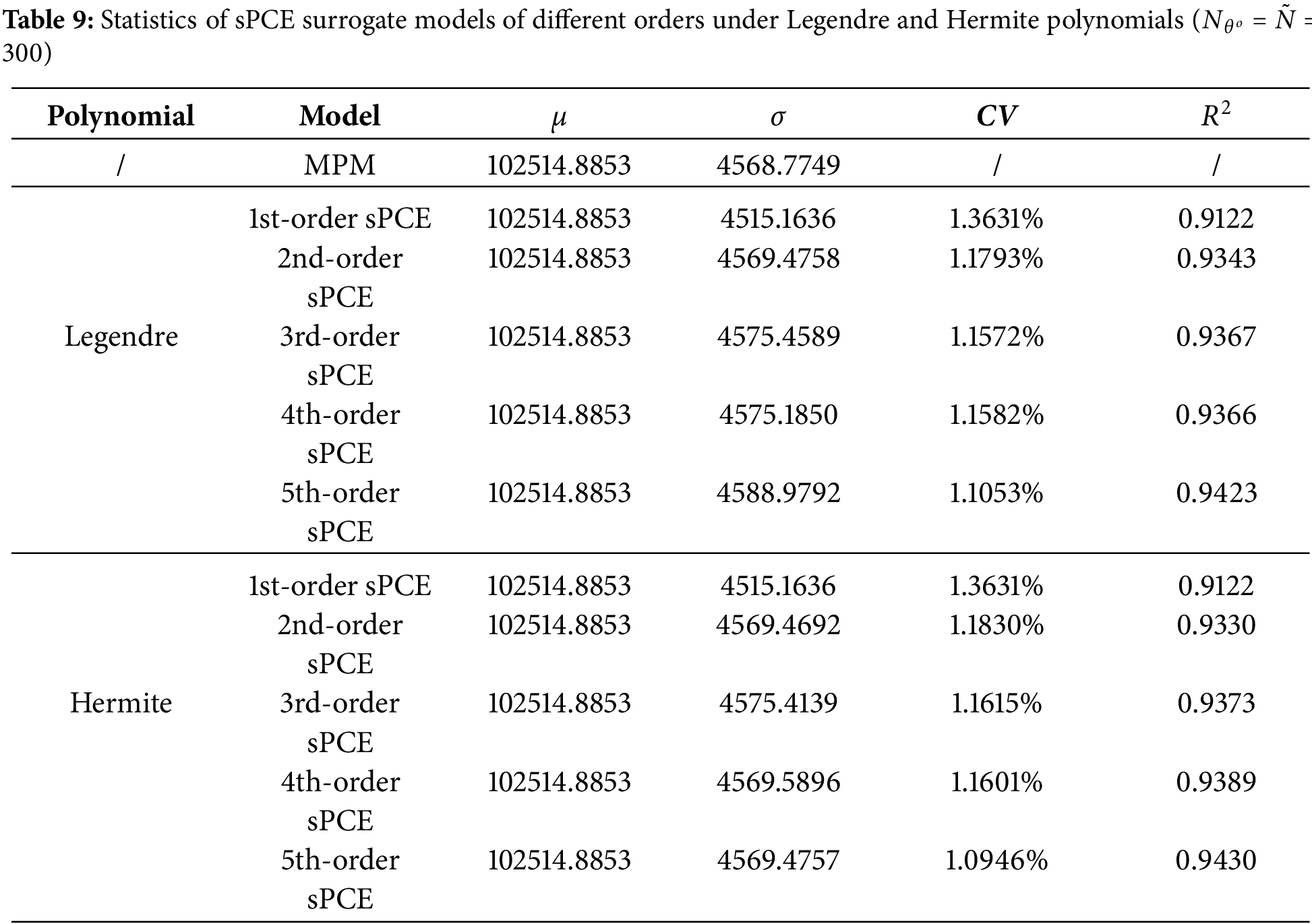
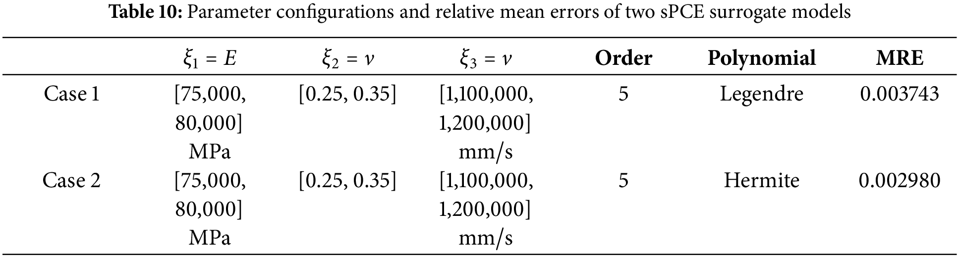
Table 10 shows the parameter configurations and relative mean errors (RME) of the two sPCE surrogate models. The orthogonal polynomials are chosen for Legendre and Hermite, and the models both have low RMEs, indicating that the models have good accuracy. Case 1 was selected for the sPCE-FDM sensitivity analysis, and Case 1 and Case 2 were selected for the Sobol global sensitivity analysis.

As shown in Fig. 19, the first-order local sensitivity increases with E after introducing a perturbation to E. At u=0.25, it begins to decline and then slopes over the interval, indicating a transition from a negative to a positive correlation. At u=0.35, the local sensitivity shifts from a positive to a negative correlation. This emphasizes the interaction of the parameters E and u on the model output. The second-order local sensitivity fluctuates with increasing E, especially within [76,500, 78,500], which indicates that the rate of change is significantly affected in this range. The introduction of a perturbation to u results in significant fluctuations in the first-order local sensitivity of the model. The range of these fluctuations will gradually expand as u increases. The second-order local spirit shows a decreasing trend in the interval [0.28, 0.32]. It rises sharply at u>0.32, suggesting that the effect of the parameters on the rate of change intensifies as u increases. The first-order local sensitivity of the model shows a clear upward trend as v rises after introducing perturbations to v, and generally stays at a low level. However, the second-order local sensitivity is more pronounced for specific values of E and u, suggesting that the effect of v on the rate of change is greater in this range.

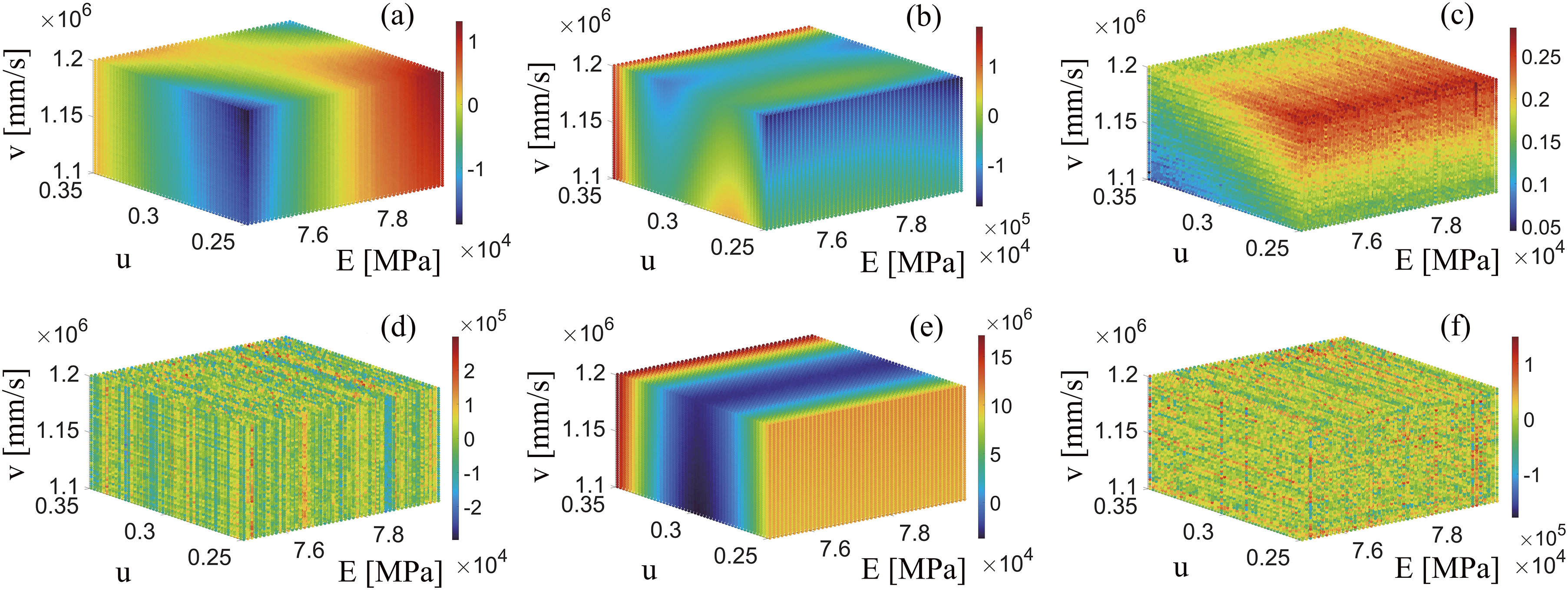
Figure 19: The sPCE surrogate model of Case 1 is used to compare the local sensitivity of sPCE-FDM for different variables: (a) first-order local sensitivity of E, (b) first-order local sensitivity of u, (c) first-order local sensitivity of v, (d) second-order local sensitivity of E, (e) second-order local sensitivity of u, (f) second-order local sensitivity of v

It can be seen in Fig. 20 that the global sensitivity analysis of the model is performed using sPCE-FDM. The effects of E and u on the overall sensitivity of the model are more pronounced when small perturbations are applied to the three input parameters (E, u, and v) at the same time, while the effects of the changes in v are relatively small. The use of 3rd-order or higher order surrogate models helps to better represent the sensitivity information and raw data.

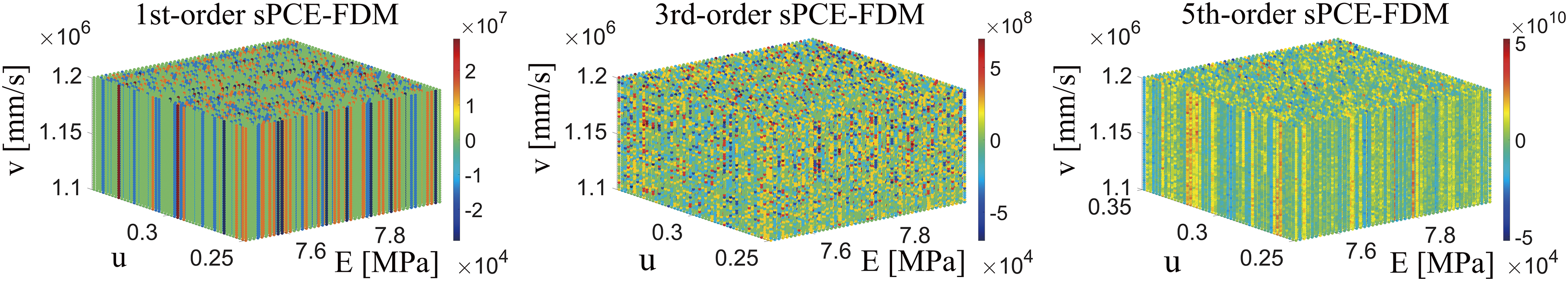
Figure 20: Comparison of sPCE-FDM global sensitivities for trivariate surrogate models of different orders under Case 1

To further explore the extent to which the three variables influence the objective function, global sensitivity analysis was carried out for the calculation of the Sobol index. Fig. 21 demonstrates the global sensitivity of the three parameters under Case 1 and Case 2. It can be seen that the results of choosing different orthogonal polynomials to construct the sPCE under the same training dataset are the same. The results of each input variable in order of results from largest to smallest are: u>E>v. Therefore, Poisson’s ratio is the main factor causing the fluctuation of strain energy. GSA is more suitable for analyzing the interactions among the variables of the structural dynamic system under uncertainty compared to LSA.

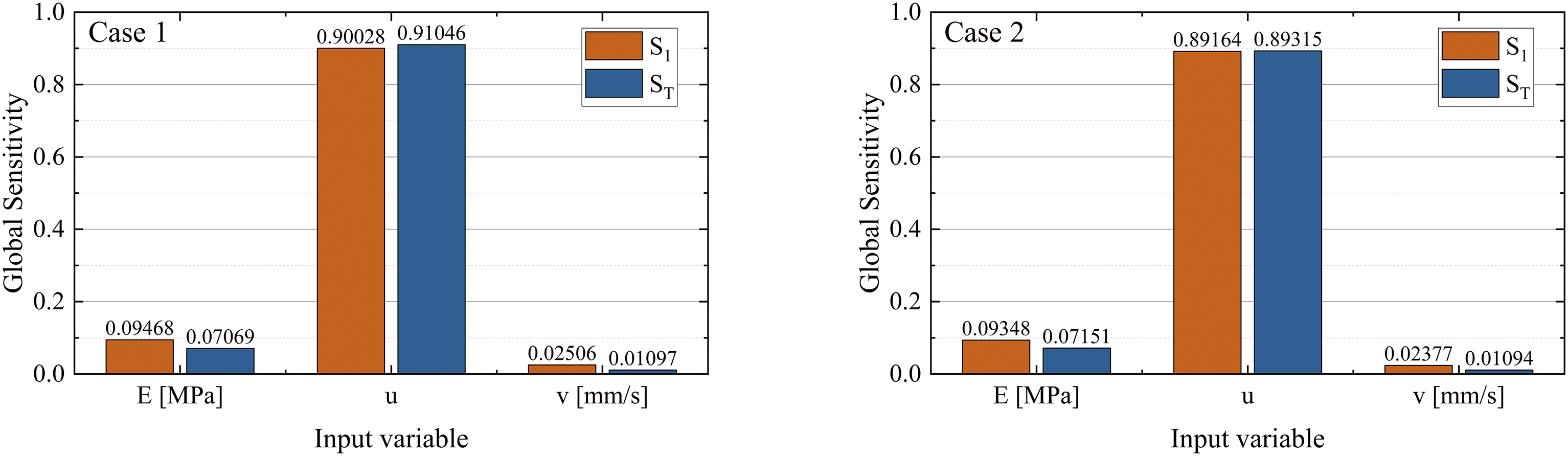
Figure 21: Sobol global sensitivity for Case 1 and Case 2

5  Conclusion

This study explores the application of MPM in structural dynamics problems, using it to simulate collisions, vibrations, and penetrations. While MPM offers high accuracy compared to other numerical simulation methods, its long single computation time presents challenges for Monte Carlo simulation and sensitivity analysis. To address this, a new approach for constructing response surface models is proposed to accelerate the MPM computational process. After comparing SVM-RBF, DT, and GPR methods, examples demonstrate that the proposed adaptive RGA for constructing sPCE achieves high accuracy and computational efficiency. The utility of local and global sensitivity analysis based on sPCE, which integrates the FDM and Sobol methods, is shown to effectively evaluate structural dynamics responses under complex conditions. This advancement not only enhances computational efficiency in structural dynamics but also provides a robust tool for understanding and optimizing such systems. In the future, sensitivity analysis methods based on MPM and sPCE are expected to play a crucial role in applied mathematical modeling, including material characterization, structural performance evaluation, and system reliability studies. These applications will extend across automotive, aerospace, civil engineering, and manufacturing fields, promoting a deeper understanding and optimization of complex engineering systems.

Despite the significant improvements in computational efficiency offered by the proposed method, constructing sPCE surrogate models for high-dimensional complex structures still requires a large training dataset, which is time-consuming to compute. Therefore, future research will focus on addressing these issues to further enhance the efficiency of the model.

Acknowledgement: The authors would like to thank the anonymous reviewers and the editors of the journal. Your constructive comments have improved the quality of this paper.

Funding Statement: The authors appreciate the financial support from the National Natural Science Foundation of China (Grant Nos. 52174123 & 52274222).

Author Contributions: The authors confirm contribution to the paper as follows: study conception and design: Wenpeng Li, Zhenghe Liu; data collection: Yujing Ma, Zhuxuan Meng, Vinh Phu Nguyen; analysis and interpretation of results: Wenpeng Li, Ji Ma, Weisong Liu; draft manuscript preparation: Wenpeng Li, Yujing Ma. All authors reviewed the results and approved the final version of the manuscript.

Availability of Data and Materials: Data will be made available on request.

Ethics Approval: Not applicable.

Conflicts of Interest: The authors declare no conflicts of interest to report regarding the present study.

Appendix A: Adaptive Randomized Greedy Algorithm for sPCE

Appendix B: Surrogate Model Configurations

References

1. Chen Z, Lai SK, Yang Z. AT-PINN: advanced time-marching physics-informed neural network for structural vibration analysis. Thin-Walled Struct. 2024;196:111423. doi:10.1016/j.tws.2023.111423. [Google Scholar] [CrossRef]

2. Zuo H, Bi K, Zhu S, Ma R, Hao H. On the dynamic characteristics of using track nonlinear energy sinks for structural vibration control. Eng Struct. 2024;302:117436. doi:10.1016/j.engstruct.2023.117436. [Google Scholar] [CrossRef]

3. Liu Z, Sun S, Cheng AH, Wang Y. A fast multipole accelerated indirect boundary element method for broadband scattering of elastic waves in a fluid-saturated poroelastic domain. Int J Num Analyt Meth Geomech. 2018;42(18):2133–60. doi:10.1002/NAG.2848. [Google Scholar] [CrossRef]

4. Sun S, Liu Z, Cheng AH. Indirect boundary element method for modelling 2-D poroelastic wave diffraction by cavities and cracks in half space. Int J Num Analyt Meth Geomech. 2021;45(14):2048–77. doi:10.1002/nag.3255. [Google Scholar] [CrossRef]

5. Sulsky D, Chen Z, Schreyer HL. A particle method for history-dependent materials. Comput Methods Appl Mech Eng. 1994;118(1–2):179–96. doi:10.1016/0045-7825(94)90112-0. [Google Scholar] [CrossRef]

6. Sulsky D, Kaul A. Implicit dynamics in the material-point method. Comput Methods Appl Mech Eng. 2004;193(12–14):1137–70. doi:10.1016/j.cma.2003.12.011. [Google Scholar] [CrossRef]

7. Zhang X, Sze K, Ma S. An explicit material point finite element method for hyper-velocity impact. Int J Num Meth Eng. 2006;66(4):689–706. doi:10.1002/nme.1579. [Google Scholar] [CrossRef]

8. Lian Y, Zhang X, Zhou X, Ma Z. A FEMP method and its application in modeling dynamic response of reinforced concrete subjected to impact loading. Comput Methods Appl Mech Eng. 2011;200(17–20):1659–70. doi:10.1016/j.cma.2011.01.019. [Google Scholar] [CrossRef]

9. Ma S, Zhang X, Lian Y, Zhou X. Simulation of high explosive explosion using adaptive material point method. Comput Model Eng Sci. 2009;39(2):101–24. doi:10.3970/cmes.2009.039.101. [Google Scholar] [CrossRef]

10. Ma Z, Zhang X, Huang P. An object-oriented MPM framework for simulation of large deformation and contact of numerous grains. Comput Model Eng Sci. 2010;55(1):61–88. doi:10.3970/cmes.2010.055.061. [Google Scholar] [CrossRef]

11. García-Sánchez G, Mancho AM, Wiggins S. A bridge between invariant dynamical structures and uncertainty quantification. Commun Nonlinear Sci Numer Simul. 2022;104(1):106016. doi:10.1016/j.cnsns.2021.106016. [Google Scholar] [CrossRef]

12. Formalik F, Shi K, Joodaki F, Wang X, Snurr RQ. Exploring the structural, dynamic, and functional properties of metal-organic frameworks through molecular modeling. Adv Funct Mater. 2024;34(43):2308130. doi:10.1002/adfm.202308130. [Google Scholar] [CrossRef]

13. Sun ZZ, Zhang Q, Gao Gh. Finite difference methods for nonlinear evolution equations. Berlin, Germany: Walter de Gruyter GmbH & Co KG; 2023. Vol. 8. [Google Scholar]

14. Odreitz K, Musil M, Deutschmann B. Morris sensitivity analysis on conducted emissions of an inverting buck-boost converter. In: 2024 IEEE Joint International Symposium on Electromagnetic Compatibility, Signal & Power Integrity: EMC Japan/Asia-Pacific International Symposium on Electromagnetic Compatibility (EMC Japan/APEMC Okinawa). Ginowan, Japan: IEEE; 2024. p. 665–8. [Google Scholar]

15. Asghari H, Topol H, Markert B, Merodio J. Application of the extended Fourier amplitude sensitivity testing (FAST) method to inflated, axial stretched, and residually stressed cylinders. Appl Mathem Mech. 2023;44(12):2139–62. doi:10.1007/s10483-023-3060-6. [Google Scholar] [CrossRef]

16. Tansar H, Duan HF, Mark O. Global sensitivity analysis of bioretention cell design for stormwater system: a comparison of VARS framework and Sobol method. Amsterdam, Netherlands: Elsevier; 2023. [Google Scholar]

17. Wan HP, Ren WX, Todd MD. Arbitrary polynomial chaos expansion method for uncertainty quantification and global sensitivity analysis in structural dynamics. Mech Syst Signal Process. 2020;142(8–10):106732. doi:10.1016/j.ymssp.2020.106732. [Google Scholar] [CrossRef]

18. Chen X, Shen Z, Liu X. Structural dynamics model updating with interval uncertainty based on response surface model and sensitivity analysis. Inverse Prob Sci Eng. 2019;27(10):1425–41. doi:10.1080/17415977.2018.1554656. [Google Scholar] [CrossRef]

19. Dong Y, Grabe J. Large scale parallelisation of the material point method with multiple GPUs. Comput Geotec. 2018;101(4):149–58. doi:10.1016/j.compgeo.2018.04.001. [Google Scholar] [CrossRef]

20. Wang D, Wang B, Yuan W, Liu L. Investigation of rainfall intensity on the slope failure process using GPU-accelerated coupled MPM. Comput Geotech. 2023;163(1):105718. doi:10.1016/j.compgeo.2023.105718. [Google Scholar] [CrossRef]

21. Zeng Z, Zhang H, Zhang X, Liu Y, Chen Z. An adaptive peridynamics material point method for dynamic fracture problem. Comput Methods Appl Mech Eng. 2022;393(3):114786. doi:10.1016/j.cma.2022.114786. [Google Scholar] [CrossRef]

22. Huang P, Zhang X, Ma S, Huang X. Contact algorithms for the material point method in impact and penetration simulation. Int J Num Meth Eng. 2011;85(4):498–517. doi:10.1002/nme.2981. [Google Scholar] [CrossRef]

23. Pisner DA, Schnyer DM. Support vector machine. In: Machine learning. Amsterdam, Netherlands: Elsevier; 2020. p. 101–21. doi:10.1016/B978-0-12-815739-8.00006-7. [Google Scholar] [CrossRef]

24. Charbuty B, Abdulazeez A. Classification based on decision tree algorithm for machine learning. J Appl Sci Technol Trends. 2021;2(1):20–8. doi:10.38094/jastt20165. [Google Scholar] [CrossRef]

25. Wang J. An intuitive tutorial to Gaussian processes regression. Comput Sci Eng. 2023;25:4–11. [Google Scholar]

26. Li YF, Cao MS, Tran-Ngoc H, Khatir S, Wahab MA. Multi-parameter identification of concrete dam using polynomial chaos expansion and slime mould algorithm. Comput Struct. 2023;281:107018. doi:10.1016/j.compstruc.2023.107018. [Google Scholar] [CrossRef]

27. Tosin M, Côrtes AM, Cunha A. A tutorial on sobolglobal sensitivity analysis applied to biological models. Netw Syst Biol: Appl Dis Model. 2020;32:93–118. [Google Scholar]

28. Pan L, Novák L, Lehkỳ D, Novák D, Cao M. Neural network ensemble-based sensitivity analysis in structural engineering: comparison of selected methods and the influence of statistical correlation. Comput Struct. 2021;242:106376. doi:10.1016/j.compstruc.2020.106376. [Google Scholar] [CrossRef]

29. Gamboa F, Klein T, Lagnoux A. Sensitivity analysis based on Cramér-von Mises distance. SIAM/ASA J Uncert Quantificat. 2018;6(2):522–48. doi:10.1137/15M1025621. [Google Scholar] [CrossRef]

30. Novák L. On distribution-based global sensitivity analysis by polynomial chaos expansion. Comput Struct. 2022;267(4):106808. doi:10.1016/j.compstruc.2022.106808. [Google Scholar] [CrossRef]

31. Novák L, Sharma H, Shields MD. Physics-informed polynomial chaos expansions. J Comput Phys. 2024;506(6):112926. doi:10.1016/j.jcp.2024.112926. [Google Scholar] [CrossRef]

32. Blatman G, Sudret B. Efficient computation of global sensitivity indices using sparse polynomial chaos expansions. Reliabil Eng Syst Safety. 2010;95(11):1216–29. doi:10.1016/j.ress.2010.06.015. [Google Scholar] [CrossRef]

33. Chen L, Huang H. Global sensitivity analysis for multivariate outputs using generalized RBF-PCE metamodel enhanced by variance-based sequential sampling. Appl Mathem Modell. 2024;126:381–404. doi:10.1016/j.apm.2023.10.047. [Google Scholar] [CrossRef]

34. Novák L, Vořechovskỳ M, Sadílek V, Shields MD. Variance-based adaptive sequential sampling for polynomial chaos expansion. Comput Methods Appl Mech Eng. 2021;386(4):114105. doi:10.1016/j.cma.2021.114105. [Google Scholar] [CrossRef]

35. Su L, Tan S, Qi Y, Gu J, Ji Y, Wang G, et al. An improved orthogonal matching pursuit method for denoising high-frequency ultrasonic detection signals of flip chips. Mech Syst Signal Process. 2023;188(10):110030. doi:10.1016/j.ymssp.2022.110030. [Google Scholar] [CrossRef]

36. Baptista R, Stolbunov V, Nair PB. Some greedy algorithms for sparse polynomial chaos expansions. J Computat Physics. 2019;387(5):303–25. doi:10.1016/j.jcp.2019.01.035. [Google Scholar] [CrossRef]

37. Arachchige CN, Prendergast LA, Staudte RG. Robust analogs to the coefficient of variation. J Appl Statist. 2022;49(2):268–90. doi:10.1080/02664763.2020.1808599. [Google Scholar] [PubMed] [CrossRef]

38. Sadeghirad A, Brannon RM, Guilkey J. Second-order convected particle domain interpolation (CPDI2) with enrichment for weak discontinuities at material interfaces. Int J Numer Meth Eng. 2013;95(11):928–52. doi:10.1002/nme.4526. [Google Scholar] [CrossRef]

39. Nguyen VP, Nguyen CT, Rabczuk T, Natarajan S. On a family of convected particle domain interpolations in the material point method. Finite Elem Analy Desi. 2017;126(2):50–64. doi:10.1016/j.finel.2016.11.007. [Google Scholar] [CrossRef]

40. Soize C, Ghanem R. Physical systems with random uncertainties: chaos representations with arbitrary probability measure. SIAM J Scient Comput. 2004;26(2):395–410. doi:10.1137/S1064827503424505. [Google Scholar] [CrossRef]

41. Azhar AS, Kudus SA, Jamadin A, Mustaffa NK, Sugiura K. Recent vibration-based structural health monitoring on steel bridges: systematic literature review. Ain Shams Eng J. 2024;15(3):102501. doi:10.1016/j.asej.2023.102501. [Google Scholar] [CrossRef]

42. He L, Tao Z. Building vibration measurement and prediction during train operations. Buildings. 2024;14(1):142. doi:10.3390/buildings14010142. [Google Scholar] [CrossRef]

43. Sadeghirad A, Brannon RM, Burghardt J. A convected particle domain interpolation technique to extend applicability of the material point method for problems involving massive deformations. Int J Numer Meth Eng. 2011;86(12):1435–56. doi:10.1002/nme.3110. [Google Scholar] [CrossRef]

44. Sulsky D, Zhou SJ, Schreyer HL. Application of a particle-in-cell method to solid mechanics. Comput Phys Commun. 1995;87(1–2):236–52. doi:10.1016/0010-4655(94)00170-7. [Google Scholar] [CrossRef]

45. Coetzee CJ. The modelling of granular flow using the particle-in-cell method. Stellenbosch: University of Stellenbosch; 2004. [Google Scholar]

46. Trucano T, Grady D. Study of intermediate velocity penetration of steel spheres into deep aluminum targets. Albuquerque, NM, USA: Sandia National Labs; 1985. [Google Scholar]