
 Submit a Paper
 Propose a Special lssue
 Open Access
ARTICLE

SEIR Mathematical Model for Influenza-Corona Co-Infection with Treatment and Hospitalization Compartments and Optimal Control Strategies
1 Tandy School of Computer Science, University of Tulsa, Tulsa, OK 74104, USA
2 Department of Mathematics and Statistics, College of Science, King Faisal University, Al-Ahsa, 31982, Saudi Arabia
* Corresponding Author: Muhammad Imran. Email:
(This article belongs to the Special Issue: Advances in Mathematical Modeling: Numerical Approaches and Simulation for Computational Biology)
Computer Modeling in Engineering & Sciences 2025, 142(2), 1899-1931. https://doi.org/10.32604/cmes.2024.059552
Received 11 October 2024; Accepted 09 December 2024; Issue published 27 January 2025
 View Full Text
 Download PDF
Abstract
The co-infection of corona and influenza viruses has emerged as a significant threat to global public health due to their shared modes of transmission and overlapping clinical symptoms. This article presents a novel mathematical model that addresses the dynamics of this co-infection by extending the SEIR (Susceptible-Exposed-Infectious-Recovered) framework to incorporate treatment and hospitalization compartments. The population is divided into eight compartments, with infectious individuals further categorized into influenza infectious, corona infectious, and co-infection cases. The proposed mathematical model is constrained to adhere to fundamental epidemiological properties, such as non-negativity and boundedness within a feasible region. Additionally, the model is demonstrated to be well-posed with a unique solution. Equilibrium points, including the disease-free and endemic equilibria, are identified, and various properties related to these equilibrium points, such as the basic reproduction number, are determined. Local and global sensitivity analyses are performed to identify the parameters that highly influence disease dynamics and the reproduction number. Knowing the most influential parameters is crucial for understanding their impact on the co-infection’s spread and severity. Furthermore, an optimal control problem is defined to minimize disease transmission and to control strategy costs. The purpose of our study is to identify the most effective (optimal) control strategies for mitigating the spread of the co-infection with minimum cost of the controls. The results illustrate the effectiveness of the implemented control strategies in managing the co-infection’s impact on the population’s health. This mathematical modeling and control strategy framework provides valuable tools for understanding and combating the dual threat of corona and influenza co-infection, helping public health authorities and policymakers make informed decisions in the face of these intertwined epidemics.Keywords
Coronavirus or COVID-19 first reported in Wuhan, China, in late 2019 [1,2]. The World Health Organization officially declared the COVID-19 pandemic in March 2020 [3,4], following a series of devastating coronaviruses, such as SARS-CoV and MERS-CoV, that had already spread globally [5,6]. The coronavirus can lead to a deadly cytokine storm, similar to previous coronaviruses [7–9]. The available evidence indicates that the primary mode of transmission of the coronavirus among individuals is through the release of respiratory droplets during activities such as sneezing and coughing [10]. The incubation period for the coronavirus disease typically ranges from 2 to 14 days, with an average of 5 to 6 days [11]. Influenza, commonly called the flu, is an infectious respiratory disease caused by the influenza virus [12,13]. During seasonal pandemics and epidemics, influenza spreads widely throughout the world. Apart from pandemic influenza, there is a global influenza outbreak every year that causes between 3 and 5 million cases of severe disease and between 250,000 and 500,000 fatalities [14]. The time it takes for the signs and symptoms of influenza to appear is about 2 days but might range from 1 to 4 days [15].
Concerns about the possibility of a twin epidemic of influenza and corona have persisted since the start of the pandemic. Many cases have been reported where individuals had both SARS-CoV-2 and influenza [16]. Up to 20% of corona patients, according to some research [17], can have co-infections with other respiratory viruses. The influenza season and the corona pandemic pose a significant threat to public health. Both viruses share similar transmission characteristics and clinical symptoms, causing respiratory infections [17]. The interplay between influenza and corona viruses is a major concern, with fatalities among people infected with both viruses being twice as high as those infected with the new coronavirus [16,17].
Co-infection between corona and other respiratory pathogens is more common in the USA and China, with 7% of SARS-CoV-2-positive patients sharing the burden of co-infection [17]. The clinical signs of corona and influenza include coughing, runny noses, sore throats, fevers, headaches, and fatigue [16,17]. Those who are infected with either virus can experience varied levels of illness, including some who show no symptoms, only minor symptoms, or severe disease [17]. Both the flu and corona can have severe consequences, including pneumonia, respiratory failure, acute respiratory distress syndrome, sepsis, heart attacks or strokes, multiple organ failure, severe inflammation, and even death [18,19].
Both coronavirus and influenza are single-stranded encapsulated RNA viruses; the former contain a positive sense RNA strand and the latter a negative one [20]. Both have comparable infection sites in the upper respiratory tracts (URT) and lower respiratory tracts (LRT). While influenza URT infections are highly transmissible but have a low pathogenicity, influenza LRT infections can produce more severe symptoms [20]. Furthermore, both viruses can spread directly from person to person or indirectly through close contact. Their routes of transmission are comparable and include droplet, aerosol, and self-inoculation by hand contamination [16,17,20]. Co-infection can affect the disease prognosis, increase therapeutic intolerance, and severely compromise the immune system of the host. One of the most important area of epidemiology has been the study of the co-existence and co-infection of multiple diseases [21,22]. To assess the dynamics of co-infection and estimate the treatment facilities, epidemiological models are very helpful. Numerous research works focus on the coexistence of two infectious agents in vulnerable hosts [22–26].
There is a considerable body of work in the literature focusing on coronavirus, influenza, and their co-infection. Epidemiologists are consistently striving to provide comprehensive insights into these epidemics and develop effective control strategies with minimal costs. In [9], the authors formulated an extended susceptible-exposed-symptomatic-asymptomatic-superspreader-quarantine-recovered (SEIAPQR) mathematical model, incorporating two non-pharmaceutical optimal control strategies: quarantine and self-precautions. In [21], the authors constructed a model for co-infection of coronavirus and influenza, introducing vaccination compartments for COVID-19, Influenza, and corona-influenza co-infection. They analyzed the impact of vaccinations, including booster doses for COVID-19, and offered a detailed analysis of influenza-corona co-infection, exploring the effects of transmission, cure, or treatment dynamics. Similarly, in [22], the authors proposed a mathematical model for corona-influenza co-infection, dividing the entire model into three susceptible-exposed-infected-recovered (SEIR) submodels with a vaccination compartment. The dynamics of each submodel are analyzed individually to understand the complete model. Finally, an optimal control strategy is defined in [22] with three optimal controls: non-pharmaceutical strategy (minimization of infectious interactions), vaccine for corona, and vaccination for influenza, respectively.
To investigate the co-dynamics of influenza and corona co-infection, we divide the total population into eight distinct time-dependent classes or compartments: susceptible
The format of this manuscript is as follows: We explore the development of the influenza-corona co-infection model (Section 2). The essential characteristics of the solution are discussed, including the presence of uniqueness and positive bounded solutions (Section 3). We analyze the equilibrium points and the reproduction number (
We divide the total population, denoted as
and flow of co-infection through compartments is shown in Fig. 1. The transmission and translation rates (
•
•
•
•
•
•
•
•
•
•
•
•
•
•
•
•
•
•
•
•
•
•
•
•
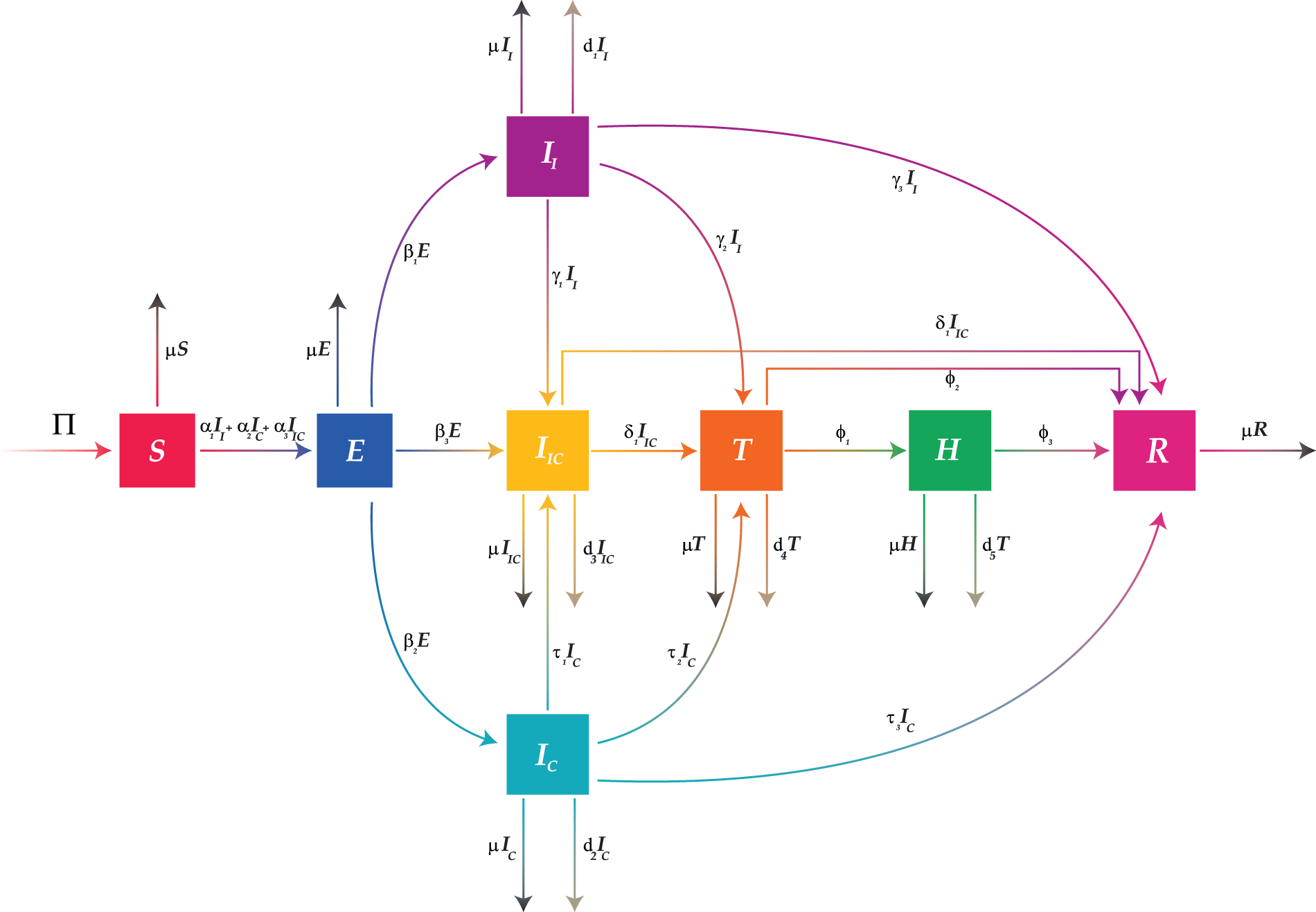
Figure 1: Flow diagram of the proposed influenza-corona co-infection model (Eq. (2))
We model the transmission of influenza-corona co-infection by the following system of non-linear differential equations.
with the non-negative initial conditions:
The above autonomous system can be written in compact form as:
where
and
respectively.
3 Theoretical Properties and Proofs
The fundamental characteristics of the proposed mathematical model, such as the existence of a unique solution and a positive, bounded solution in a feasible region is demonstrated in this section.
Theorem 3.1. The co-infection model (Eq. (2)) has a bounded solution,
Proof. By differentiating Eq. (1) w.r.t time
with
Since,
By using the properties of the Laplace transformation and partial fraction on inequality (6), we get
The Laplace inverse transformation yield us
Thus,
Thus,
Theorem 3.2. With the positive initial conditions, the co-infection model (Eq. (2)) has a positive solution
Proof. Since,
As we already proved all the state variables are bounded by
Thus,
Applying the Laplace transformation gives
Now, using the inverse Laplace transformation
Since
◼
Before proving the existence and uniqueness properties of the solution of the proposed model, we define following fundamental theorems:
Theorem 3.3. [27] Suppose
Theorem 3.4. The model (Eq. (3)) has a unique solution on
Proof. Since, all the state variables are assumed to be continuously differentiable on
To prove Lipschitz condition, we need to prove that
It is clear that all the partial derivatives,
Thus, we have proved that the proposed model (Eq. (2)) has a unique, positive, and bounded solution (Fig. 2).
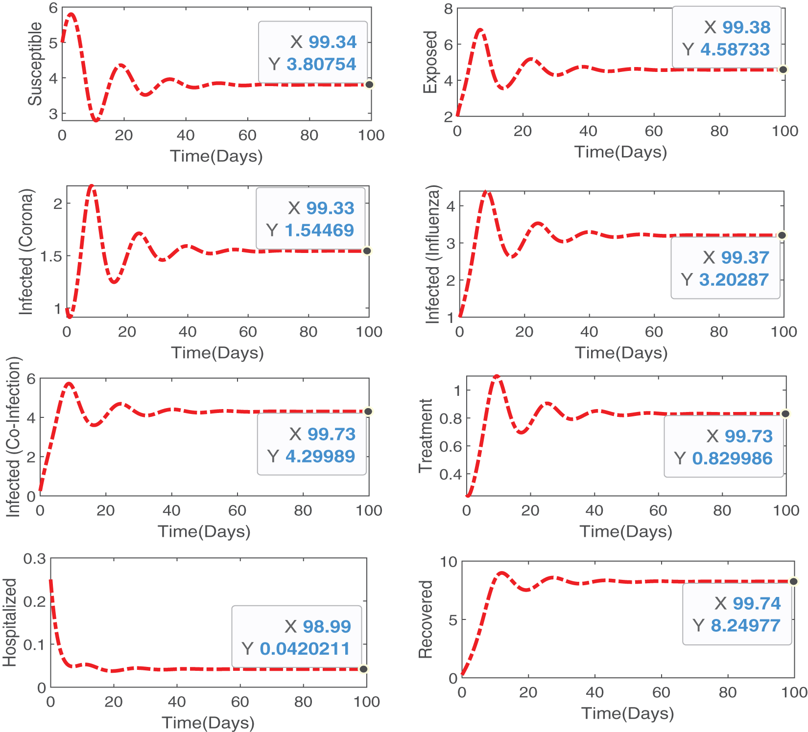
Figure 2: Numerical simulations illustrating theoretical results proved analytically, that our proposed model is bounded and positive within a feasible region and has a unique solution
4 Equilibrium Points and Associated Properties
In this section, we determine the important equilibrium points and the properties associated with these equilibrium points. Specifically, we drive the reproduction number
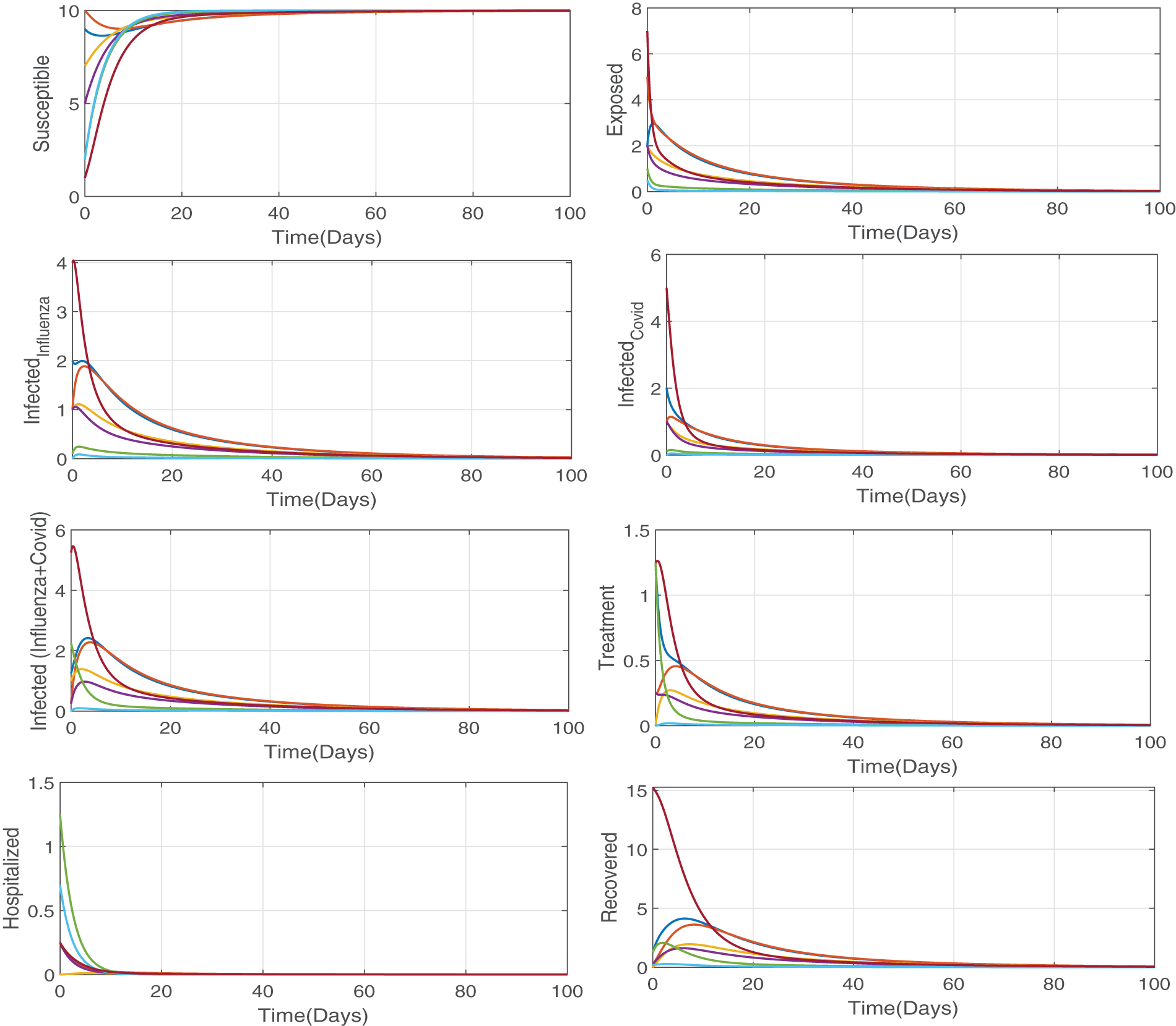
Figure 3: Numerical simulation illustrating the our proposed model (Eq. (2)) is stable at disease free equilibrium point when
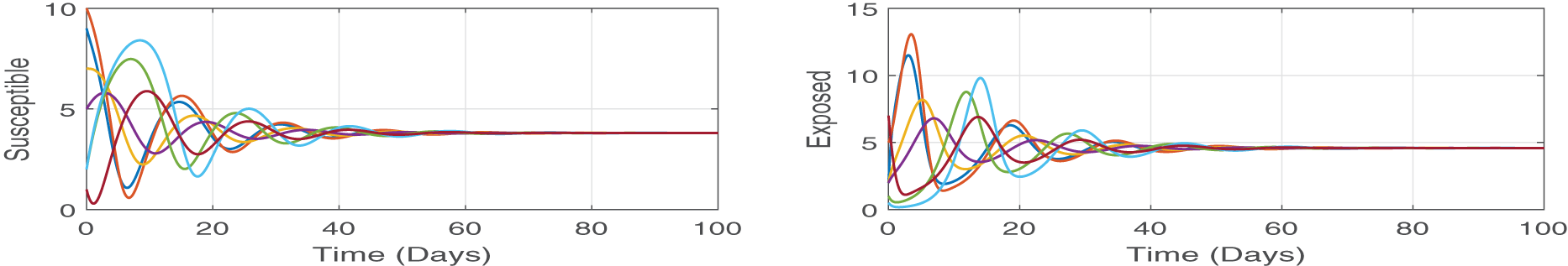
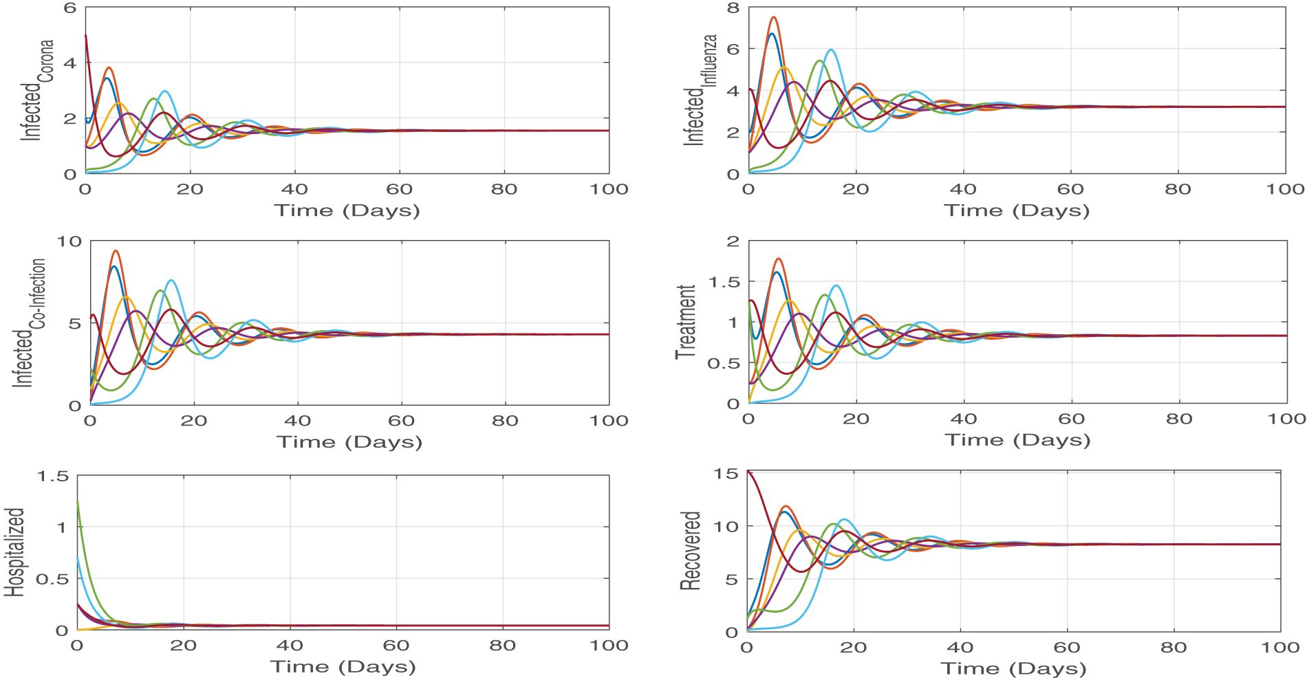
Figure 4: We numerically solve the system by using different initial values, but all the solutions approach same point which is the endemic point. These simulations demonstrate the state theorem (Theorem 4.4) that the proposed model (Eq. (2)) is stable at endemic equilibrium point (
4.1 Equilibrium Points and Reproduction Number
To find equilibrium points, we consider the rate of change of all the state variables equal to zero, i.e.,
A critical epidemiological metric that quantifies the average number of secondary infections produced by a single infectious person in a fully susceptible (disease free) population is the reproduction number
where,
The Jacobian of the matrices
Thus, the spectral radius of
where
Here
Theorem 4.1. The proposed model (Eq. (2)) is locally asymptotically stable (LAS) at the disease free equilibrium point
Proof. This theorem can be proved by using the Jacobian matrix approach. For this purpose, we need to find Jacobian matrix at DFE point, i.e.,
As we know that, a system is said to be stable at an equilibrium if all the eigenvalues are negative at this equilibrium point and unstable otherwise. Therefore, we calculate the eigenvalues of the above matrix with the help of Maple software:
Since all the eigenvalues are negatives when
In order to show that the DFE point
Theorem 4.2. The disease free equilibrium (DFE) point
where
Proof. Let
If
From Eq. (19), as
where
and
It is evident that
4.2.1 Endemic Equilibrium Point
To find endemic equilibrium point (
where
Theorem 4.3. The Model (Eq. (2)) is locally asymptotically stable (LAS) at endemic equilibrium point
Proof. Now, we linearized the proposed model (Eq. (2)) at endemic equilibrium point (
Since all the eigenvalues are negative when
Theorem 4.4. The endemic equilibrium (EE) point
Proof. Let
Taking the derivative of Eq. (23) w.r.t time
By replacing the values of the time derivatives of state variables of the model (Eq. (2)), we get
where
and
For
Now, if we put EE point,
and
Thus,
Thus, LaSalle’s invariance principle [28] guarantee that the endemic equilibrium (EE) point
Sensitivity analysis is needed to design efficient viral control strategies. Our goal is to find parameters that are extremely sensitive to
We calculate the sensitivity indices for every parameter used in
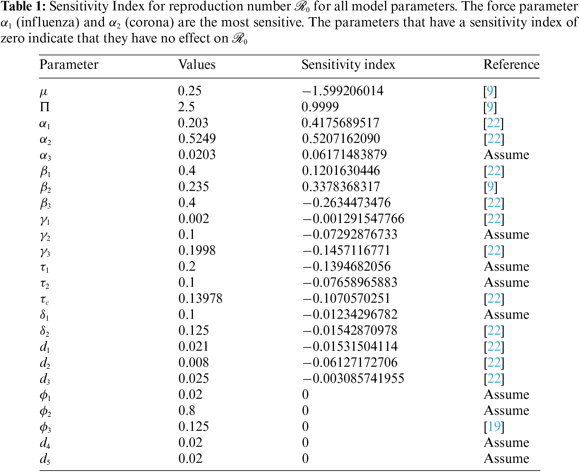
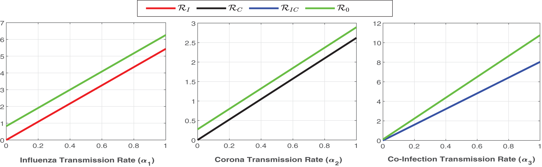
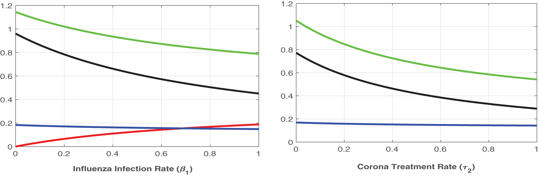
Figure 5: Plot of
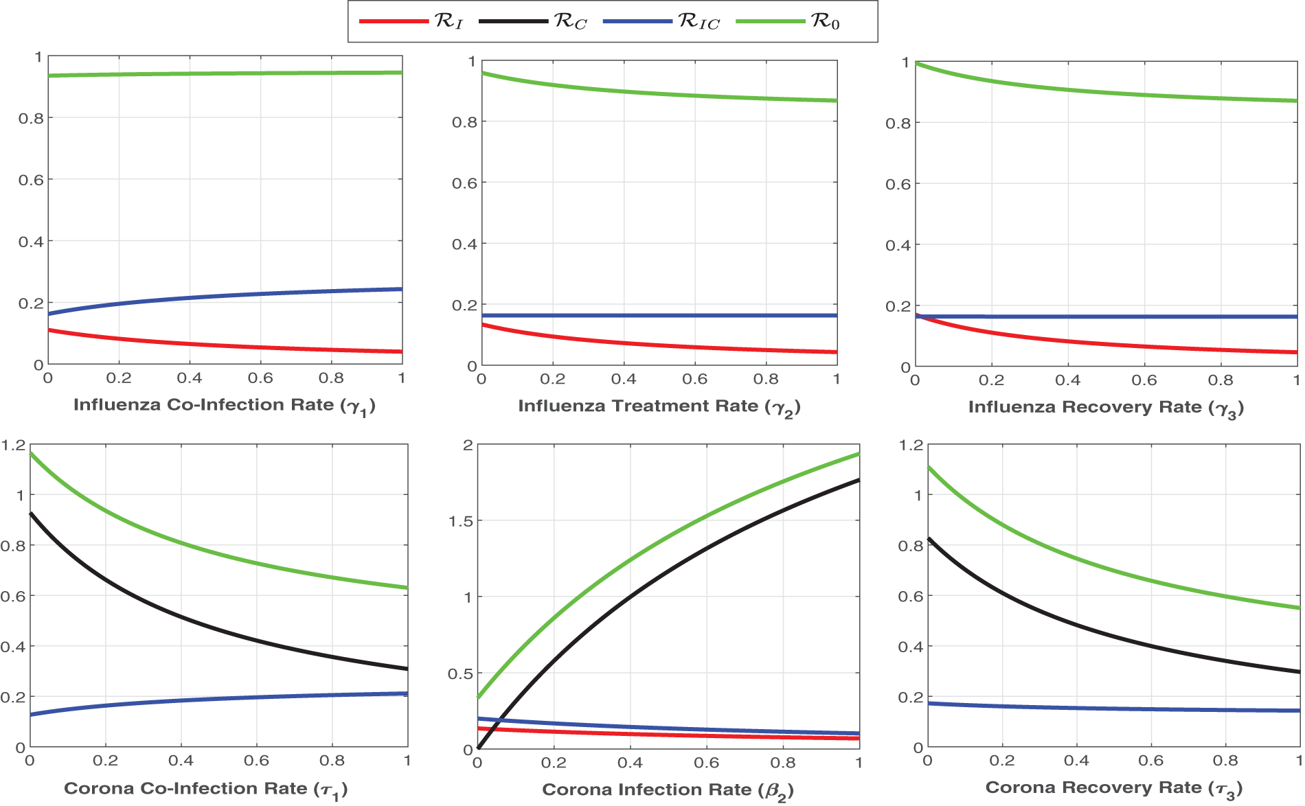
Figure 6: Plot of
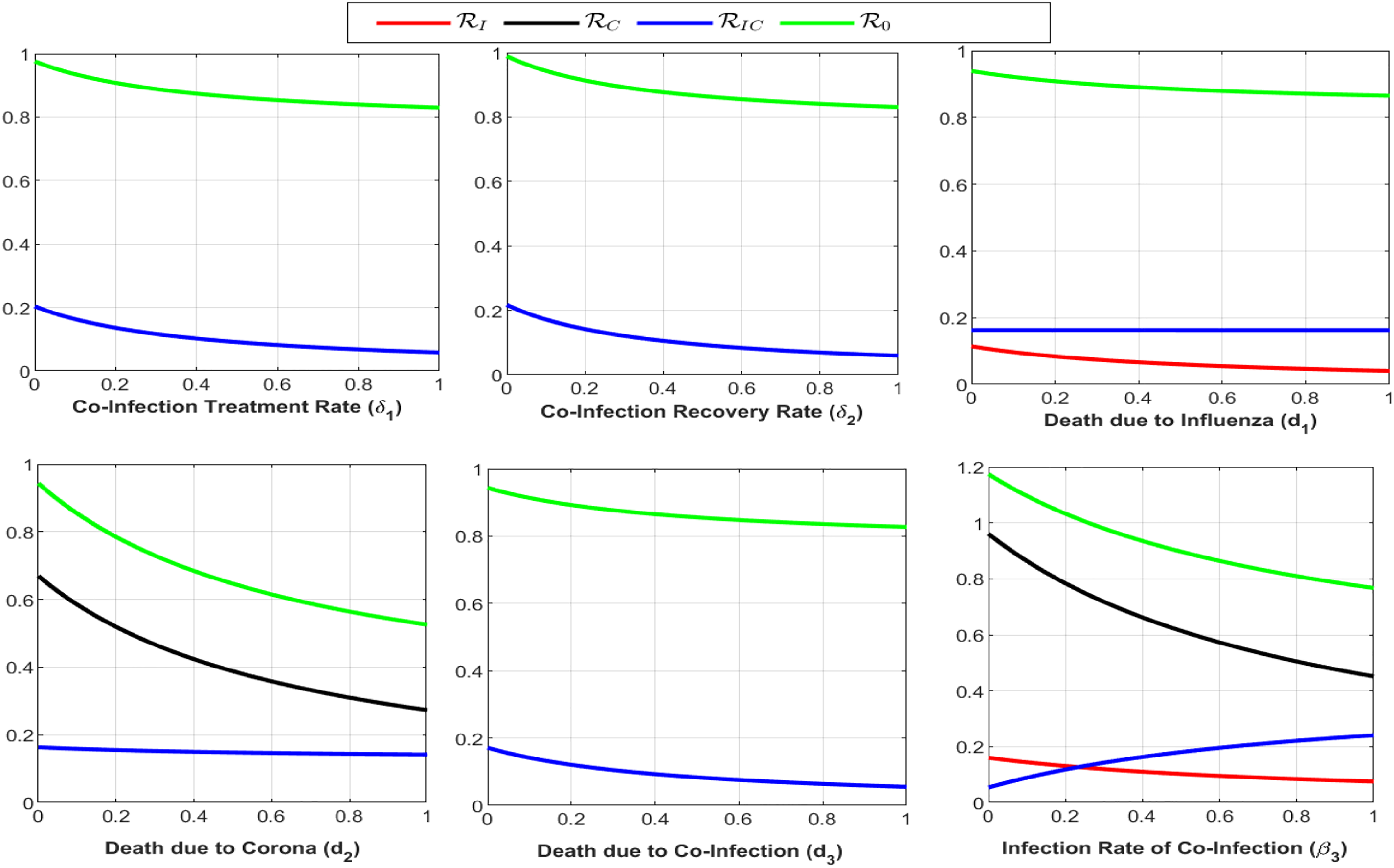
Figure 7: Plot of reproduction numbers
In this section, we will provide a comprehensive analysis of different control analysis. We will perform both the fixed control and optimal control analysis with different control parameters [33–37].
To provide insightful information and realistic analysis, we update the proposed model (Eq. (2)) with a new non-pharmaceutical parameter
6.2 Effect of Different Control Levels
Here we investigate the influence of self-precaution and treatment rates on the dynamics of state variables in the updated model (Eq. (26)), with a particular focus on those representing infection within the population. Employing various precautions and treatment levels spanning from 0% to 80%, we examine their effects on disease control. The findings indicate a decline in the number of infectious cases as the treatment level increases. Consequently, we can deduce that an elevated treatment rate for infectious classes correlates with a reduction in infection. It is clear from Figs. 8–10, treatment can reduce infection, but it cannot permanently eradicate the co-infection disease. On the other hand, self-precaution, (e.g., social distancing, the wearing of a mask, and the regular use of handwash) is an efficient non-pharmaceutical way to protect oneself and to help to eradicate the disease from the population (Fig. 11). Based on analysis of different aspects of the disease dynamics and cost of controls, self-precaution is the best policy to eradicate the disease. The combined effect of all treatment parameters with and without self-precautions will be presented in the next section.
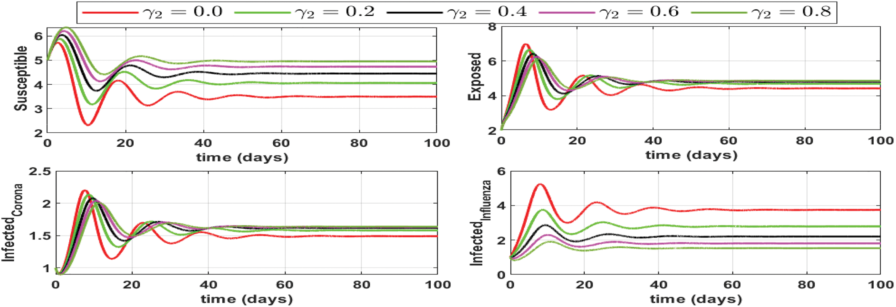
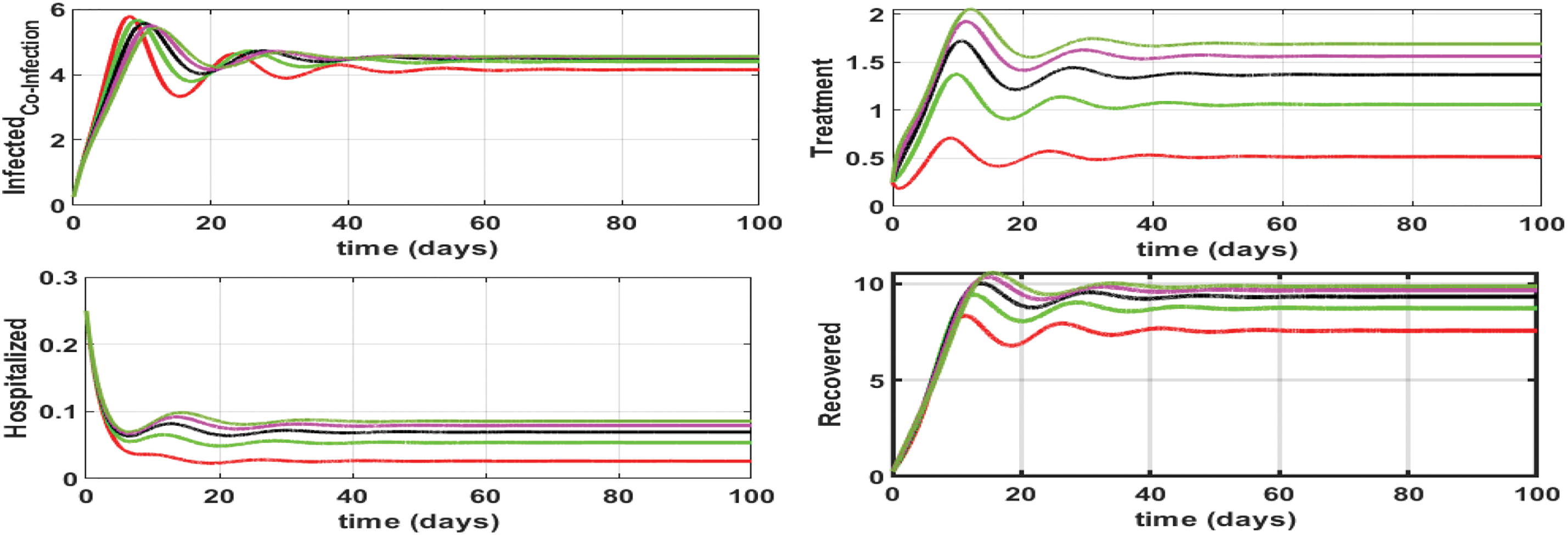
Figure 8: Impact of influenza treatment rate (
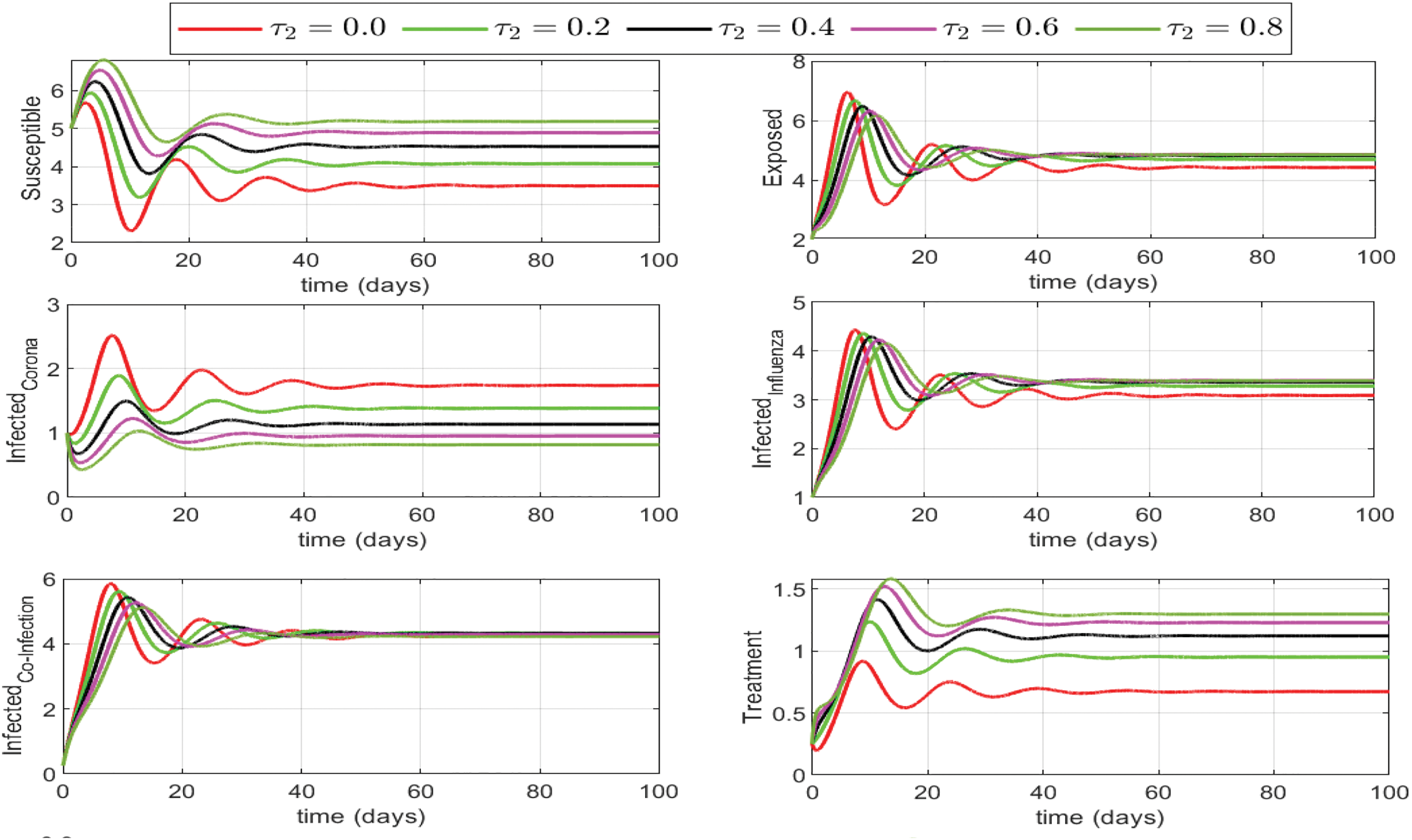
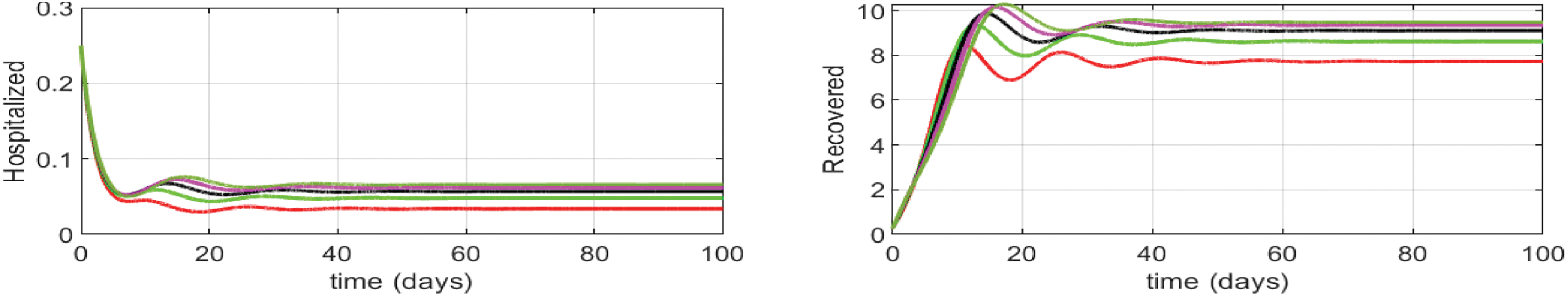
Figure 9: Different levels of treatment rate
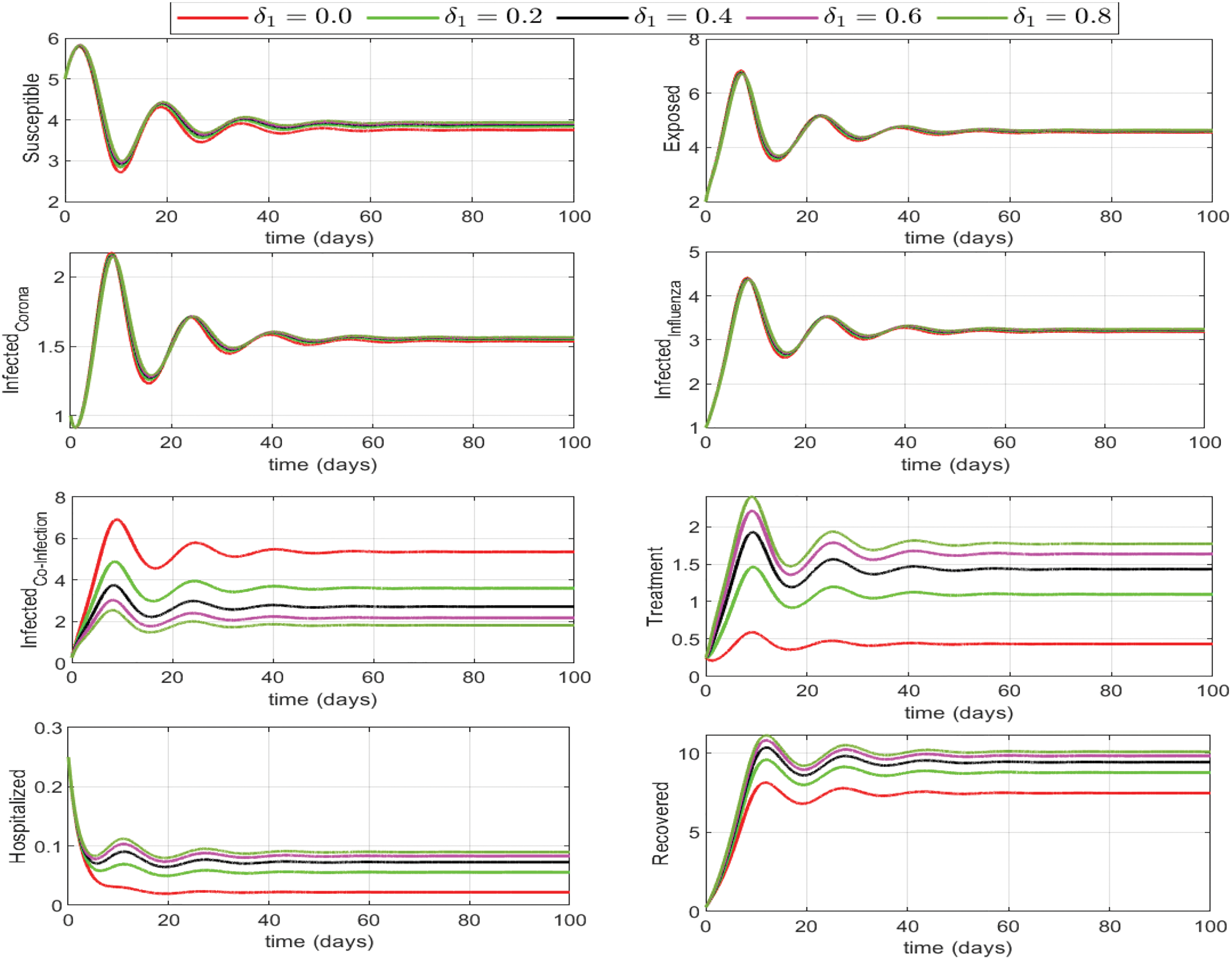
Figure 10: Effect of influenza-corona co-infection treatment rate
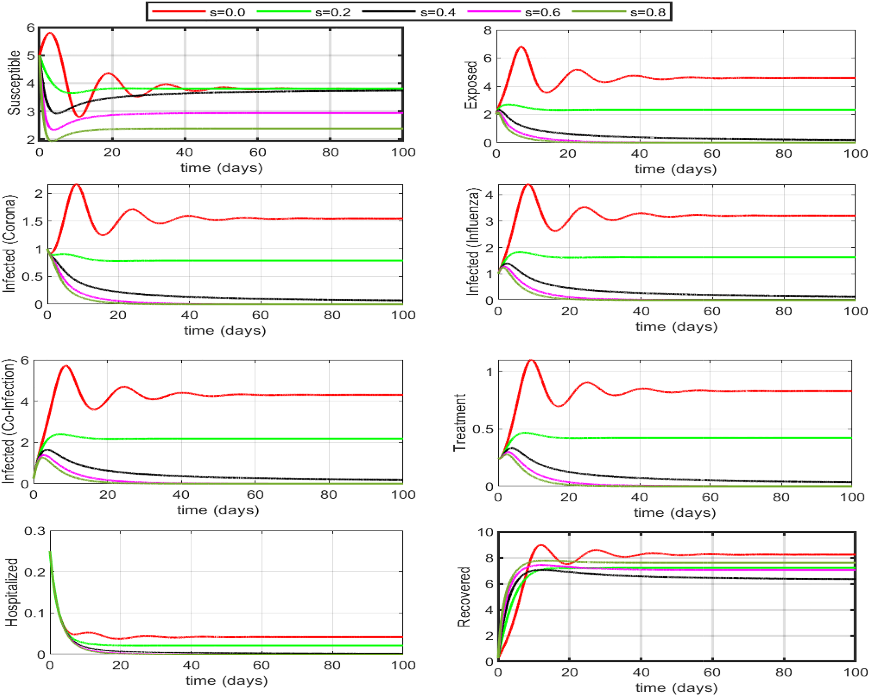
Figure 11: Impact of self-precaution on the dynamics assuming that if someone is taking precautions, they are recovered by default. If 50% to 60% (self-precaution s = 0.5 or 0.6) of the susceptible population is aware of the disease and is taking safety measures (i.e., social distancing, hand washing, etc.), then the disease will die out within a few days. Self-precaution not only helps eradicate the disease but also decreases the number of under-treatments individuals and the burden on hospitalized
In this section, we will define an optimal control problem to find the optimal treatment rates and self-precaution measures as time-dependent controls. We perform optimal control analysis for model (Eq. (26))using the Pontryagin maximum principle (PMP). The objective functional to be minimized is defined as follows:
where
The object is to find the optimal control
6.3.1 Necessary Optimality Conditions
For PMP optimization, we construct the following Hamiltonian
We denote the state variables by
The First condition of optimality is given by
The PMP gives us the following expressions for the controls
Under the max-min bounds, we update the controls to have
Using the second optimality condition
We get the following adjoint equations
with
In the first case, we take all three treatment controls (
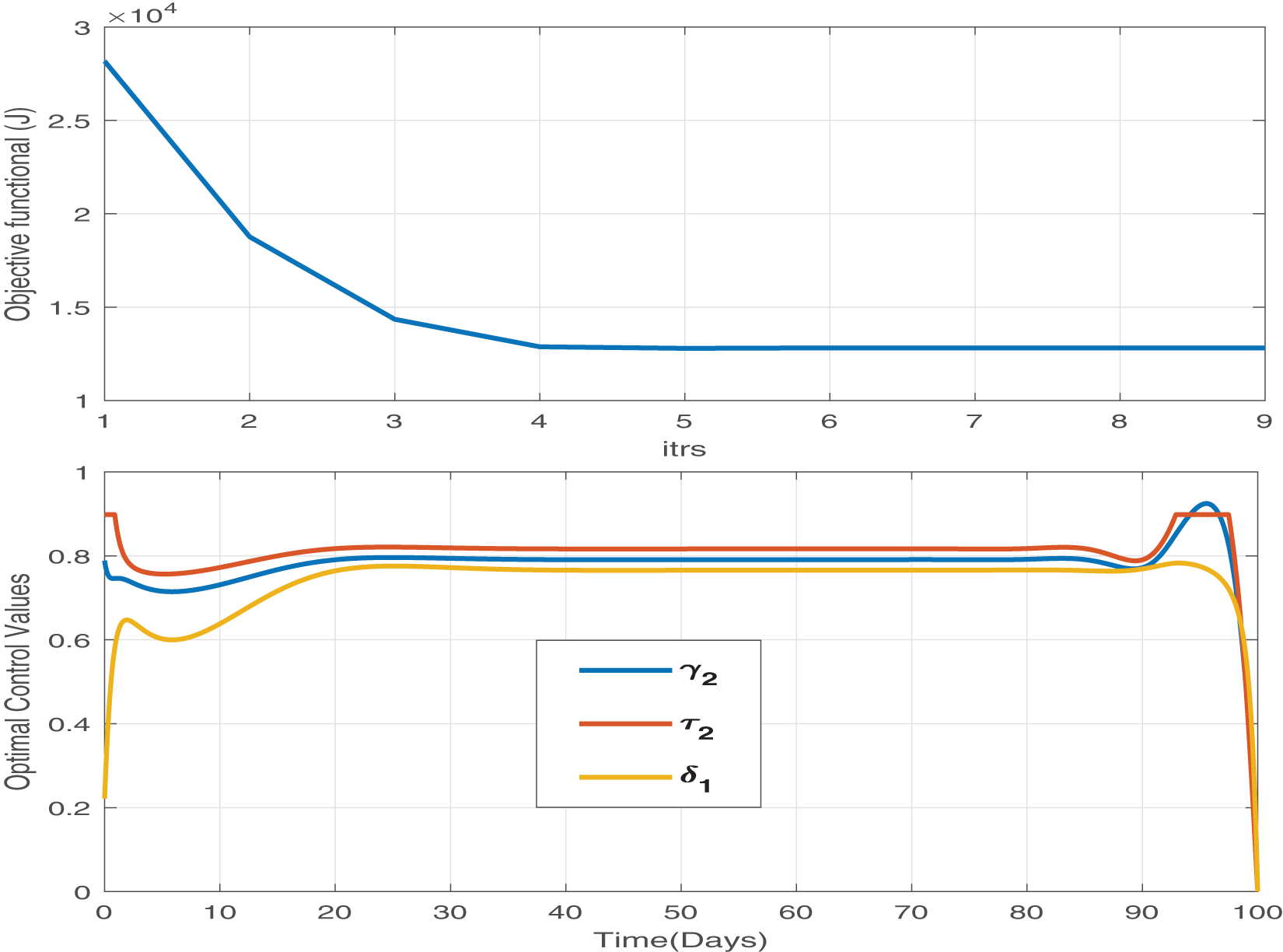
Figure 12: The objective functional and the corresponding optimal control values for parameters
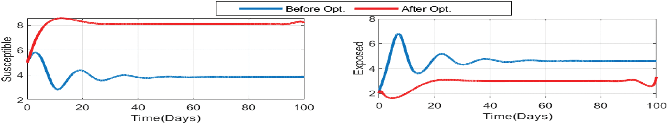
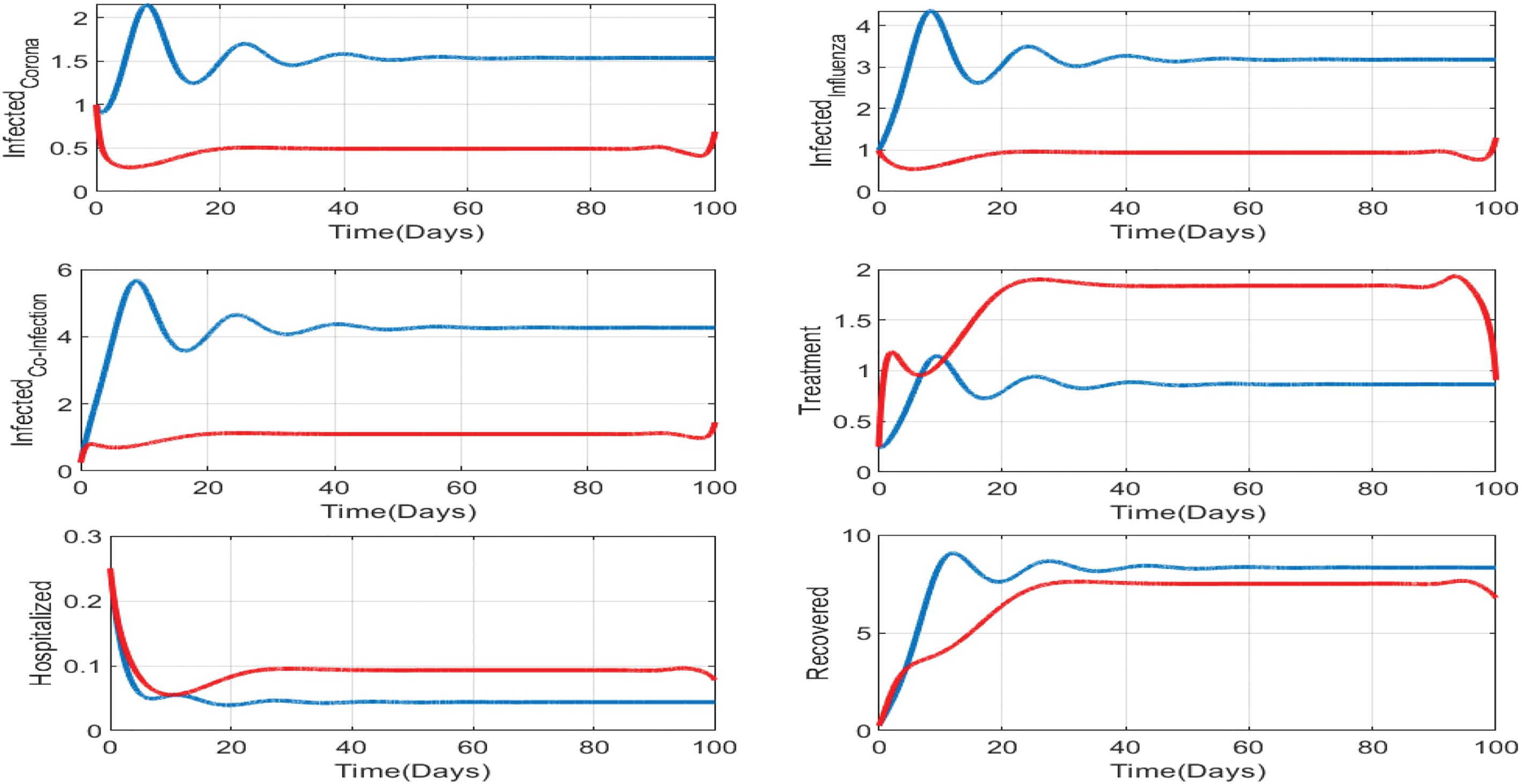
Figure 13: Impact of treatments on the susceptible, exposed, influenza-infective, and corona-infective populations. The red line represents the dynamics of each state variable before the use of optimal treatment controls, and the red line represents the dynamics after applying the optimal controls for 100 days
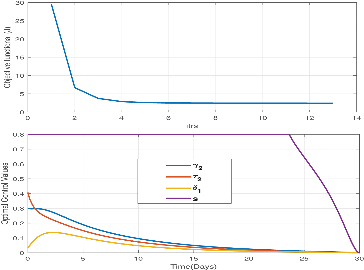
Figure 14: We adopt both pharmaceutical (treatment) and non-pharmaceutical (self-precaution) optimal controls and analyze the effect of this control strategy. This is the best control strategy. It minimizes the burden of disease as well as the cost of treatment. We obtain the minimum value of the objective functional in only 13 iterations, and the maximum level of treatments is 40% and for a very short time
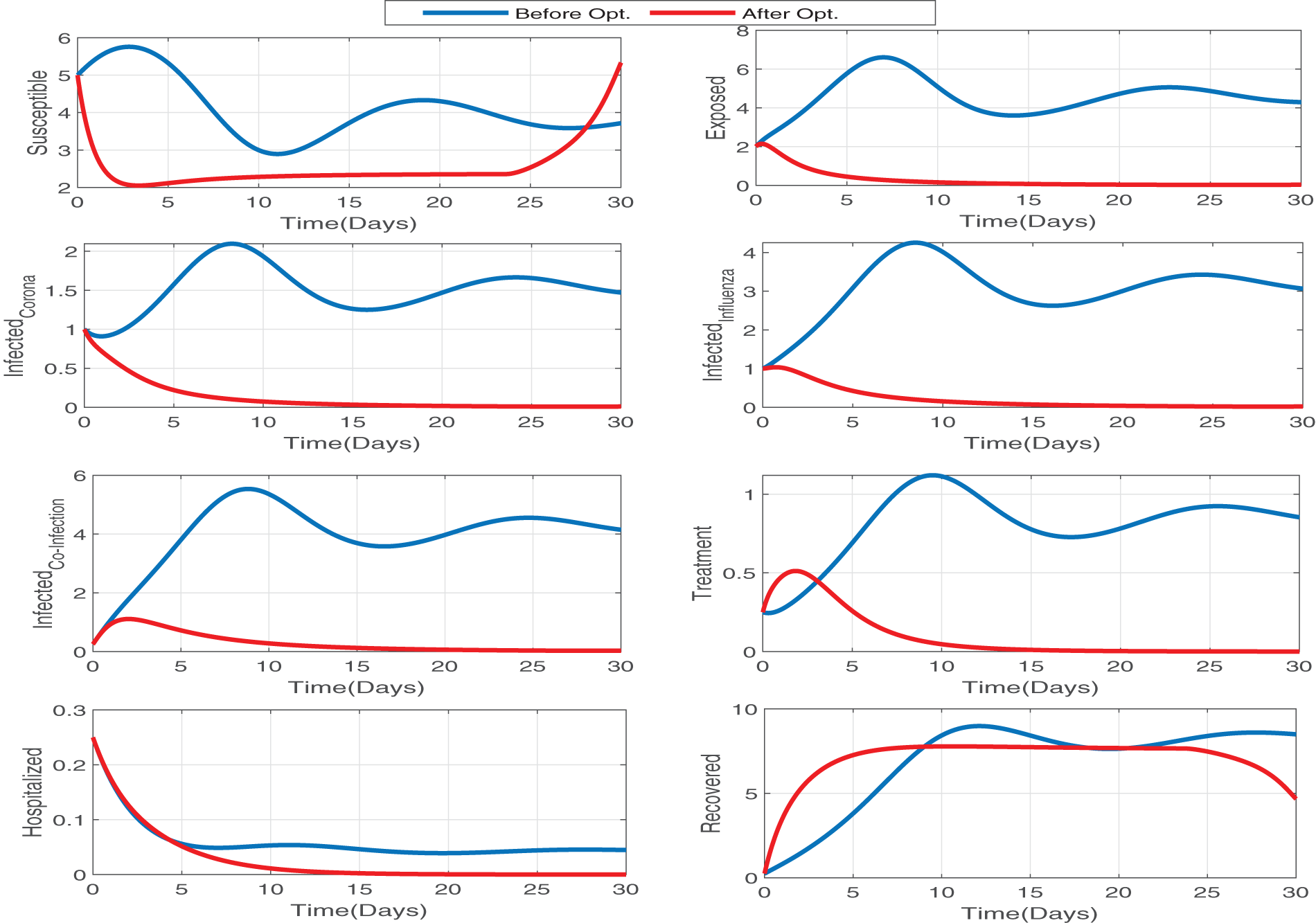
Figure 15: The impact of optimal treatments and self-precaution control has a great impact on the susceptible, exposed, influenza infectious, and corona infectious populations. The blue and red lines represent the dynamics without and with optimal controls. Since red lines reach zero in all the infectious compartments in a very short time, this optimal control is very effective
In this manuscript, we have proposed a new
In our upcoming research, we will use a fractional model to provide a thorough depiction of the co-infection dynamics of influenza and coronavirus. This model will use Caputo-Fabrizio (CF) and Atangana-Baleanu Caputo (ABC) derivative operators to represent the intricate interactions between the two illnesses. Furthermore, we will incorporate numerous intervention options, such as immunization, into this framework. Our research will go beyond analyzing the success of these interventions, suggesting optimal approaches to vaccination and hospitalization using a fractional-order optimal control problem. This will enable us to identify the most effective strategies for lowering the co-infection burden on the healthcare systems and improving patient health. In addition to the above, the proposed influenza-corona co-infection model offers valuable insights into dynamics and control strategies but has limitations. It simplifies complex biological and socio-behavioral processes, assumes homogeneous population mixing, and overlooks multi-strain infections, resistance, and co-infections with other diseases, affecting real-world applicability.
Acknowledgement: We would like to thank NASA Oklahoma Established Program to Stimulate Competitive Research (EPSCoR) Infrastructure Development, “Machine Learning Ocean World Biosignature Detection from Mass Spec” (PI: Brett McKinney), and Tandy School of Computer Science, University of Tulsa.
Funding Statement: This work was partly supported by NASA Oklahoma Established Program to Stimulate Competitive Research (EPSCoR) Infrastructure Development, “Machine Learning Ocean World Biosignature Detection from Mass Spec” (PI: Brett McKinney), Grant No. 80NSSC24M0109, and Tandy School of Computer Science, University of Tulsa.
Author Contributions: The authors confirm contribution to the paper as follows: Muhammad Imran: Conceptualization, Data curation, Formal analysis, Software, Validation, Writing—original draft. Brett McKinney: Supervision, Data curation, Formal analysis, Investigation, Project administration, Resources, Writing—review & editing. Azhar Iqbal Kashif Butt: Software, Validation, Visualization, Writing—review & editing. All authors reviewed the results and approved the final version of the manuscript.
Availability of Data and Materials: Data sharing not applicable to this article as no datasets were generated or analyzed during the current study.
Ethics Approval: Not applicable.
Conflicts of Interest: The authors declare no conflicts of interest to report regarding the present study.
References
1. World of Health Organization. Novel Coronavirus (2019-nCoV)–SITUATION REPORT-1. 2020. Available from: https://www.who.int/docs/default-source/coronaviruse/situation-reports/20200121-sitrep-1-2019-ncov.pdf. [Accessed 2024]. [Google Scholar]
2. World of Health Organization. WHO Director-General’s opening remarks at the media briefing on COVID-19–11 March 2020. Available from: https://www.who.int/director-general/speeches/detail/who-director-general-s-opening-remarks-at-the-media-briefing-on-covid-19—11-march-2020. [Accessed 2023]. [Google Scholar]
3. Hu B, Huang S, Yin L. The cytokine storm and COVID-19. J Med Virol. 2021 Jan;93(1):250–6. doi:10.1002/jmv.26232. [Google Scholar] [PubMed] [CrossRef]
4. Hui DS, Azhar EI, Madani TA, Ntoumi F, Koch R, Dar O, et al. The continuing 2019-nCoV epidemic threat of novel corona viruses to global health: the latest 2019 novel coronavirus outbreak in Wuhan, China. Int J Infect Dis. 2020;91:264–6. [Google Scholar] [PubMed]
5. Abioye AI, Peter OJ, Addai E, Oguntolu FA, Ayoola TA. Modeling the impact of control strategies on malaria and COVID-19 coinfection: insights and implications for integrated public health interventions. Qual Quant. 2024;58(4):3475–95. doi:10.1007/s11135-023-01813-6. [Google Scholar] [CrossRef]
6. Ojo MM, Peter OJ, Goufo EFD, Nisar KS. A mathematical model for the co-dynamics of COVID-19 and tuberculosis. Math Comput Simul. 2023;207(3):499–520. doi:10.1016/j.matcom.2023.01.014. [Google Scholar] [PubMed] [CrossRef]
7. Kumar Ghosh J, Saha P, Kamrujjaman M, Ghosh U. Transmission dynamics of COVID-19 with saturated treatment: a case study of spain. Braz J Phys. 2023;53(3):54. doi:10.1007/s13538-023-01267-z. [Google Scholar] [CrossRef]
8. Khondaker F, Kamrujjaman M, Shahidul Islam M. Optimal control analysis of COVID-19 transmission model with physical distance and treatment. Adv Biol Res. 2022;3(1):65–76. [Google Scholar]
9. Butt AIK, Imran M, Batool S, Nuwairan MA. Theoretical analysis of a COVID-19 CF-fractional model to optimally control the spread of pandemic. Symmetry. 2023;15(2):380. doi:10.3390/sym15020380. [Google Scholar] [CrossRef]
10. Mohsen A, AL-Husseiny HF, Zhou X, Hattaf K. Global stability of COVID-19 model involving the quarantine strategy and media coverage effects. AIMS Pub Health. 2020;7(3):587–605. [Google Scholar]
11. World of Health Organization. COVID-19 epidemiological update–24 November 2023. Available from: https://www.who.int/publications/m/item/covid-19-epidemiological-update-24-november-2023. [Accessed 2023]. [Google Scholar]
12. World of Health Organization. Influenza (Seasonal). 2023 Oct 3. Available from: https://www.who.int/news-room/fact-sheets/detail/influenza-(seasonal). [Accessed 2023]. [Google Scholar]
13. Taubenberger JK, Morens DM. 1918 influenza: the mother of all pandemics. Emerg Infect Dis. 2006 Jan;12(1):15–22. doi:10.3201/eid1201.050979. [Google Scholar] [PubMed] [CrossRef]
14. World of Health Organization. 70 years of GISRS–the global influenza surveillance & response system. Available from: https://www.who.int/news-room/feature-stories/detail/seventy-years-of-gisrs–the-global-influenza-surveillance—response-system. [Accessed 2024]. [Google Scholar]
15. CDC. Key Facts About Influenza (Flu). Available from: https://www.cdc.gov/flu/about/keyfacts. [Accessed 2024]. [Google Scholar]
16. Tang CY, Boftsi M, Staudt L, McElroy JA, Li T, Duong S, et al. SARS-CoV-2 and influenza co-infection: a cross-sectional study in central Missouri during the 2021–2022 influenza season. Virology. 2022 Nov;576(10):105–10. doi:10.1016/j.virol.2022.09.009. [Google Scholar] [PubMed] [CrossRef]
17. Arguni E, Supriyati E, Hakim MS, Daniwijaya EW, Makrufardi F, Rahayu A, et al. Co-infection of SARS-CoV-2 with other viral respiratory pathogens in Yogyakarta, Indonesia: a cross-sectional study. Ann Med Surg. 2022 May;77:103676. doi:10.1016/j.amsu.2022.103676. [Google Scholar] [PubMed] [CrossRef]
18. Peter OJ, Panigoro HS, Abidemi A, Ojo MM, Oguntolu FA. Mathematical model of COVID-19 pandemic with double dose vaccination. Acta Biotheor. 2023;71(2):9. doi:10.1007/s10441-023-09460-y. [Google Scholar] [PubMed] [CrossRef]
19. Musa R, Peter OJ, Oguntolu FA. A non-linear differential equation model of COVID-19 and seasonal influenza co-infection dynamics under vaccination strategy and immunity waning. Healthcare Anal. 2023;4(5):100240. doi:10.1016/j.health.2023.100240. [Google Scholar] [CrossRef]
20. World of Health Organization. Coronavirus disease (COVID-19similarities and differences between COVID-19 and influenza. Available from: https://www.who.int/news-room/questions-and-answers/item/coronavirus-disease-covid-19-similarities-and-differences-with-influenza. [Accessed 2024]. [Google Scholar]
21. Bhowmick S, Sokolov IM, Lentz HHK. Decoding the double trouble: a mathematical modelling of co-infection dynamics of SARS-CoV-2 and influenza-like illness. Biosystems. 2023;224(11):104827. doi:10.1016/j.biosystems.2023.104827. [Google Scholar] [PubMed] [CrossRef]
22. Ojo MM, Benson TO, Peter OJ, Goufo EFD. Nonlinear optimal control strategies for a mathematical model of COVID-19 and influenza co-infection. Phys A: Stat Mech Appl. 2022;607(1):128173. doi:10.1016/j.physa.2022.128173. [Google Scholar] [PubMed] [CrossRef]
23. Butt AIK, Imran M, McKinney BA, Batool S, Aftab H. Mathematical and stability analysis of dengue malaria co-infection with disease control strategies. Mathematics. 2023;11(22):4600. doi:10.3390/math11224600. [Google Scholar] [CrossRef]
24. Butt AIK, Aftab H, Imran M, Ismaeel T, Arab M, Gohar M, et al. Dynamical study of lumpy skin disease model with optimal control analysis through pharmaceutical and non-pharmaceutical controls. Eur Phys J Plus. 2023;138(11):1048. doi:10.1140/epjp/s13360-023-04690-y. [Google Scholar] [CrossRef]
25. Ojo MM, Benson TO, Shittu AR, Goufo EFD. Optimal control and cost-effectiveness analysis for the dynamic modeling of Lassa fever. J Math Comput Sci. 2022;12:136. [Google Scholar]
26. Ayele TK, Doungmo Goufo EF, Mugisha S. Mathematical modeling of HIV/AIDS with optimal control: a case study in Ethiopia. Results Phys. 2021;26(1):104263. doi:10.1016/j.rinp.2021.104263. [Google Scholar] [CrossRef]
27. Burden R, Faires J. Numerical analysis. 9th ed. Boston, MA, USA: Cengage Learning; 2011. [Google Scholar]
28. Butt AIK, Chamaleen DBD, Batool S, Nuwairan MA. A new design and analysis of optimal control problems arising from COVID-19 outbreak. Math Meth Appl Sci. 2023;46(16):16957–82. [Google Scholar]
29. Martchva M. An introduction to mathematical epidemiology. New York, NY, USA: Springer; 2015. [Google Scholar]
30. Butt AIK, Imran M, Aslam J, Batool S, Batool S. Computational analysis of control of hepatitis B virus disease through vaccination and treatment strategies. PLoS One. 2023;18(10):e0288024. doi:10.1371/journal.pone.0288024. [Google Scholar] [PubMed] [CrossRef]
31. Castillo-Chavez C, Feng Z. Global stability of an age-structure model for TB and its applications to optimal vaccination strategies. Math Biosci. 1998 Aug 1;151(2):135–54. doi:10.1016/S0025-5564(98)10016-0. [Google Scholar] [PubMed] [CrossRef]
32. Ahmad W, Rafiq M, Abbas M. Mathematical analysis to control the spread of Ebola virus epidemic through voluntary vaccination. Eur Phys J Plus. 2020;135(10):1–34. Article no. 775. doi:10.1140/epjp/s13360-020-00683-3. [Google Scholar] [CrossRef]
33. Musa SS, Zhao S, Abdulrashid I, Qureshi S, Colubri A, He D. Evaluating the spike in the symptomatic proportion of SARS-CoV-2 in China in 2022 with variolation effects: a modeling analysis. Infect Dis Model. 2024;9(2):601–17. doi:10.1016/j.idm.2024.02.011. [Google Scholar] [PubMed] [CrossRef]
34. Abdulrashid I, Friji H, Topuz K, Ghazzai H, Delen D, Massoud Y. An analytical approach to evaluate the impact of age demographics in a pandemic. Stoch Environ Res Risk Ass. 2023;37(10):3691–705. doi:10.1007/s00477-023-02477-2. [Google Scholar] [PubMed] [CrossRef]
35. Abdulrashid I, Caraballo T, Han X. Effects of delays in mathematical models of cancer chemotherapy. J Pure Appl Funct Anal. 2022;7(4):1103–26. [Google Scholar]
36. Borri A, Palumbo P, Papa F, Possieri C. Optimal design of lock-down and reopening policies for early-stage epidemics through SIR-D models. Annu Rev Control. 2021;51(29):511–24. doi:10.1016/j.arcontrol.2020.12.002. [Google Scholar] [PubMed] [CrossRef]
37. Borri A, Palumbo P, Papa F. The stochastic approach for SIR epidemic models: do they help to increase information from raw data? Symmetry. 2022;14:2330. doi:10.3390/sym14112330. [Google Scholar] [CrossRef]
Cite This Article
 Copyright © 2025 The Author(s). Published by Tech Science Press.
This work is licensed under a Creative Commons Attribution 4.0 International License , which permits unrestricted use, distribution, and reproduction in any medium, provided the original work is properly cited.
 Downloads
 Citation Tools