Enhanced Multi-Object Dwarf Mongoose Algorithm for Optimization Stochastic Data Fusion Wireless Sensor Network Deployment

1  Introduction

With the development of wireless sensors and micro-electro-mechanical systems, wireless sensor networks have developed rapidly, attracting extensive attention from both academia and industry [1]. Wireless sensor networks, which consist of sensor nodes independently distributed in the detection area, were initially widely used in the military field, and are now widely used in our daily lives such as environmental monitoring, agriculture, healthcare, smart cities, industrial automation, internet of things, transportation and vehicle management, etc. [2]. Wireless sensor networks are low-cost, simple to deploy and scalable, and capable of real-time monitoring and data collection, but the sensor nodes have the problem of energy constraints, the deployment of network nodes greatly affects the overall energy consumption of the network and thus directly affects the performance of the wireless sensor network [3]. Literature [4] points out that deploying sensors has always been a great challenge for wireless sensor networks, and the effective deployment of nodes is a prerequisite for wireless sensor networks to cover the target area efficiently. Therefore, this study is dedicated to solving the deployment problem of wireless sensor networks to extend the network lifecycle, coverage, and other performance.

Coverage is a key indicator for determining the quality of wireless sensor network node deployment. Coverage can be divided into spatial coverage and temporal coverage, where spatial coverage measures the range of the target area monitored by the wireless sensor network, and temporal coverage measures whether the wireless sensor network is tracking the target on time [5]. Previous research on the deployment of wireless sensor network nodes has usually been based on simple target area coverage perception models, such as the 0–1 perception model and the probabilistic perception model [4,6–8]. However, the perception model used in practical applications usually adopts a data fusion model that fuses the perception results of multiple sensors. Data fusion models improve the accuracy of sensor monitoring and expand the coverage of wireless sensor networks. The 0–1 sensing model assumes that the sensing range of a sensor is a circle [5]. The probabilistic sensing model assumes that a sensor has two sensing radii, an inner sensing radius and an outer sensing radius. Targets within the inner sensing radius are detectable, while targets within the outer sensing radius are detected with a probability assigned by humans [9]. This makes the monitoring results of the model affected by the assigned probability. Therefore, there is a gap between the two models and the actual sensing of sensors. This paper studies the deployment of a stochastic data fusion wireless sensor network (SDFWSN), which is more in line with practical applications. This model assumes that the sensor’s perception of the signal energy emitted by the target point is affected by environmental factors such as distance, temperature, and humidity. The signal energy is negatively correlated with the distance from the sensor to the target point, and within a certain range, it decreases with increasing temperature and decreasing humidity. The final monitoring result is a fusion of the monitoring results of sensors within a certain range. This model is in line with the perception process of sensors in practice. The model mentioned in [5] is used for spatial and temporal coverage. To the best of our knowledge, this is the first time that time delay has been considered in the process of wireless network deployment optimization, and the SDFWSN model applied in this study is more realistic, making our experimental results more accurate.

Consider a deployment area with multiple dynamic target points and static sensor node candidate locations using (α,β) spatial coverage model, i.e., a target point has a probability α of being falsely detected (no target point is present but the sensor emits a positive result) and a probability β of being correctly detected (a target point is present and the sensor correctly detects the target point), where α is referred to as the false alarm rate, β is referred to as the detection rate and α∈(0,0.5)and β∈(0.5,1). The α−delay temporal coverage model is used, i.e., the average number of detection cycles from the first detection to the target provided that the network false alarm rate is not greater than α. This paper aims to reduce the false alarm rate and increase the detection rate by optimizing the deployment of the network, extending the network lifecycle, and improving the spatiotemporal coverage of the network. The problem is modeled as a multi-objective optimization problem with five objectives. Notably, this is a Non-deterministic Polynomial-time hard task [10]. When dealing with the above problem, it is best to use meta-heuristics to efficiently solve the problem [11]. DMOA is an effective swarm intelligence algorithm that can solve various optimization problems [12]. This paper designed and used an enhanced multi-objective mongoose optimization algorithm (EMODMOA) to find a feasible stochastic data fusion-based network node deployment scheme considering network lifecycle, spatial coverage, temporal coverage, detection, and false alarms. DMOA is inspired by the social behaviors of dwarf mongoose populations such as guarding, babysitting, and attacking predators [13]. The DMOA algorithm has the advantages of being simple and easy to implement and does not require excessive parameter adjustment. However, it has a slow convergence speed and is prone to local optima due to the weak balance between exploration and exploitation [14]. In this paper, the encircling and hunting strategy is highlighted by simulating the encircling and hunting habits of the dwarf mongoose. With the encircling and hunting strategy, the algorithm can successfully escape from local optima and achieve a good balance between exploration and exploitation. In this paper, the K-Nearest Neighbor (KNN) algorithm is used to select the reference points, EMODMOA is proposed, and the performance of EMODMOA is tested using the CEC2020 multi-objective multi-modal optimization benchmark function. The algorithm is used to complete the multi-objective stochastic data fusion wireless sensor.

The main contributions of this paper are as follows:

1. By simulating the biological habits of the dwarf mongoose, a strategy for encircling and hunting is proposed, which is an enhanced dwarf mongoose optimization algorithm (EDMOA) is proposed.

2. The KNN algorithm is used to select reference points, and a multi-objective dwarf mongoose optimization algorithm is established to improve the efficiency of the multi-objective algorithm.

3. A stochastic data fusion network model is established based on the original data fusion network model by considering the influence of environmental factors on the sensing effect of sensors, and the deployment of sensor nodes of this model is studied.

4. When optimizing the deployment of network nodes, maximizing the spatial coverage of the network will maximize the temporal coverage and the accuracy of monitoring as the goal to ensure the speed and quality of network monitoring.

The rest of the paper is organized as follows: Section 2 of this paper describes the literature review. Section 3 gives the construction of the SDFWSN model. Section 4 describes the construction of EMODMOA and the application of the algorithm, Section 5 performs the CEC2020 benchmark function on the proposed algorithm and Section 6 gives the experimental results and discussion. Section 7 concludes the paper and proposes future work.

2  Related Works

Several works have solved the node deployment problem in WSN systems using swarm intelligence algorithms [15]. Sections 2.1 and 2.2 provide an overview of research on WSN node deployment and DMOA, respectively.

2.1 WSN Node Deployment

Hajjej et al. [16] proposed a multi-objective flower pollination algorithm (MOFPA) for stochastic WSN scheduling. It aims to deploy a set of sensors in a target area under the condition of guaranteed network connectivity while optimizing the total network coverage and energy consumption. Wang et al. [17] employ a node scheduling scheme based on a multi-objective evolutionary algorithm to schedule heterogeneous nodes in shifts, thus extending the life cycle of the network. Non-dominated Sorting Genetic Algorithm-iii (NSGA-III) is used to optimize the deployment of WSN to reduce the network energy consumption and improve network coverage while ensuring network connectivity [18]. The deployment of WSNs in environments where obstacles are present is investigated, using a multi-objective optimization algorithm to deploy sensor nodes in a way that ensures network connectivity to maximize coverage and reduce deployment costs [19]. Saad et al. [20] addressed the deployment of WSN in 3D environments using NSGA-II. It is worth mentioning that they simulated a real space 3D model using the Bresenham line-of-sight 3D environment coverage model. Zaimen et al. [21] considered the problem of optimizing the deployment of sensor nodes in heterogeneous obstacle indoor environments, using the BIM database as well as other additional inputs (sensor node parameters) and a genetic algorithm to provide the optimal deployment. A new method based on Support Vector Regression and Genetic Algorithm is proposed for the deployment optimization problem of WSN nodes, which argues that the configuration and deployment of WSN affects almost all of their performance metrics, and the support vector regression model is utilized for the configuration of the node parameters of the Wireless Sensor Networks, and the configured node model is optimized for the deployment [22]. An enhanced multi-objective marine predator algorithm (CMOMPA) is proposed, which utilizes a Gaussian elite perturbation strategy and a learning strategy based on a competitive mechanism to generate progeny with enhanced diversity and distribution, and balances the deployment cost, connectivity, and coverage of heterogeneous WSN under specific coverage constraints [23]. The Voronoi diagram method is used to divide the monitoring area to obtain the appropriate sensing radius and communication radius, and the algorithm is used to solve the problem of deploying the wireless sensor network on 3D terrain and to improve the Quality of Service (QoS) of the wireless sensor network [24]. A resource scheduling algorithm for large-scale wireless sensor networks based on differential co-evolution and multi-objective decomposition is proposed, which is used to simultaneously optimize the position and dormant state of nodes [25]. In [26], three heuristic algorithms are used to optimize the deployment of sensor nodes, thereby maximizing the network lifetime and network coverage is divided into. The deployment of sensor nodes is optimized using an improved vampire bat optimizer, which obtains the optimal deployment location and the minimum number of sensors required by optimally splicing the sensing region with the cellular grid [27].

Looking at the current state of research at domestic and abroad, it can be found that most of the models currently studied in the literature for the deployment problem of wireless sensor networks are too simple, and there is a huge difference between them and practical applications. There are obvious differences between the currently studied sensor sensing models which mainly utilize the 0–1 sensing model, the probabilistic sensing model, the advanced sensing models, and information processing schemes adopted by the existing sensor networks; and there are few literature studies on the temporal coverage problem and the quality of network monitoring of the network. This study proposed a stochastic data fusion wireless sensor model as the wireless sensor coverage deployment model for the following reasons:

(1) The model adopts a random sensing model. Most of the traditional wireless sensor networks use a 0–1 sensing model or probabilistic sensing model, which does not consider the randomness of sensing, while sensors using a stochastic sensing model sense the signal energy of the target point will be affected by the external environment, which makes the sensor’s sensing with randomness and more realistic.

(2) The current study of wireless sensor networks for monitoring using an independent transmission model which is very different from the advanced data transmission model used in practice, this project uses a data fusion model that is more in line with the practical application, a certain range of sensors to fuse their monitoring results to obtain the final monitoring results.

2.2 DMOA

In 2022, Sadoun et al. used DMOA to improve the Long Short-Term Memory (LSTM) model to predict the properties of composite materials [28]. The model improved by DMOA has a prediction accuracy of 99%. In 2022, Akinola et al. introduced a simulated annealing algorithm to a binary variant of DMOA [29] which balanced the detection and exploitation capabilities of the algorithm. In 2022, Agushaka et al. improved DMOA by incorporating other social behaviors of dwarf mongooses, i.e., predation, mound protection, reproduction, and group splitting behaviors [30], greater enhancement of the dwarf mongoose’s exploration and exploitation capabilities, and improved convergence speed of the algorithm. In 2022, Mehmood et al. proposed a meta-heuristic algorithm for parameter estimation of autoregressive exogenous models based on DMOA [31]. The algorithm has fast convergence speed, high estimation accuracy, and strong robustness. In 2023, Agushaka et al. introduced adaptive and stochastic factors to the DMOA, which improves the exploration capability and availability of the algorithm and improves the diversity of the solution [32]. In 2022, Akinola et al. solved the high-dimensional feature selection problem using a binary version of DMOA [33]. In 2022, Alissa et al. proposed a dwarf mongoose algorithm based on machine learning-driven ransomware detection by combining DMOA with machine learning-driven ransomware detection [34], which is effective in identifying and classifying malware or ransomware. In 2022, Alrayes et al. used improved DMOA to select cluster heads of unmanned aerial vehicles to find the optimal routes to reach their destinations [35]. In 2022, Balasubramaniam et al. embedded DMOA into a lightweight deep neural network architecture for heart disease prediction [36]. In 2023, Zare et al. used DMOA to integrate the battery life, operations and maintenance cost, fuel cost and environmental cost of microgrids to determine the optimal operating parameters and improve the load capacity of microgrids [37]. In 2023, Dora et al. merged Symbiotic Organism Search (SOS) into DMOA to enhance the algorithm’s local search capability [38], solved the reactive power scheduling problem using the proposed enhanced DMOA and found the optimal settings to minimize the real power loss, total voltage variation and L-index. In 2023, Fu et al. proposed an improved DMOA which introduced the optimal leader mechanism and proposed a novel nonlinear control strategy based on sinusoidal function, which ensured the accuracy of the algorithm and at the same time improved the convergence speed of the algorithm [39]. In 2022, Abirami et al. combined DMOA with Gaussian Convolution Deep Confidence Networks for effective classification and extraction of retinal images to examine diabetic retinopathy [40]. In 2023, Almutairi et al. introduced quantum techniques to DMOA, which accelerated the convergence of the algorithm at a later stage [41]. In 2023, Rizk-Allah et al. used a modified DMOA to identify unknown parameters of an computational and physical elements model (single-phase transformer) and to evaluate the aging trend of the transformer at the hottest temperature [42].

Throughout the research status at domestic and abroad, the research on DMOA is mainly carried out in the following two aspects: one is to improve the performance of the basic algorithm for the deficiencies that exist, and a variety of different types of improved versions of DMOA have been proposed, the other is to broaden the scope of application of DMOA. With the deepening of the research, it can be found that although there are more literature on the improvement of DMOA performance, through a large number of numerical examples of experiments and comparative analysis found that DMOA still exists in the exploration and exploitation capacity is difficult to achieve the balance; easy to fall into the local optimum and late convergence of the slow speed and other shortcomings, and single-objective algorithms of the application of the scope of a certain degree of restriction. In this study, the shortcomings of the DMOA are as follows:

(1) EDMOA is proposed, which introduces nonlinear convergence factors and Markov Chain ideas in the original DMOA to accelerate the convergence speed of the algorithm, solve the problem of imbalance between the detection and exploitation capabilities, and improve the ability of the algorithm to jump out of the local optimal solution. In order to solve more practical application problems, EDMOA is designed to EMODMOA. The performance and application range of DMOA are comprehensively improved.

(2) Evaluate the performance of the proposed algorithm. Theoretically analyze the time complexity of the algorithm and test the performance of the algorithm using the CEC2020 multi-objective multi-modal optimization benchmark function.

(3) The proposed algorithm is used for the optimal deployment of SDFWSN. The results obtained in this study are of great theoretical significance and application prospects for advancing the development of the discipline of modern intelligent optimization technology.

3  Network Model and Problem Formulation

In this section, based on the data fusion wireless sensor network model proposed in [5], a stochastic data fusion network model is proposed by considering the effect of the environment on sensor sensing and defining the objective function to optimize this network model.

A data fusion network consists of many distributed sensor nodes. The key objective is to integrate dispersed information from multiple nodes to obtain more comprehensive and reliable information. First, there is data collection and pre-processing. The information collected by the sensor nodes may contain noise or redundancy due to signal attenuation. Pre-processing of the data through noise filtering, anomaly detection, and data correction provides a reliable data source for subsequent data fusion, ω(⋅) will be defined as a signal attenuation function. Second, data merging and data fusion are performed. Multiple sensor nodes may collect the same or similar data. The sensor measurements are weighted. Decision-making and reasoning are performed again. The goal of data fusion is to make decisions or reasons based on the results of data fusion. By setting a threshold, a judgment can be made based on the fusion results as to whether a target state or event has occurred. Compared with traditional wireless sensor networks, data fusion-based wireless sensor networks have stronger data transmission reliability, lower transmission latency, and wider coverage.

3.1 Description and Assumptions of the Model

3.1.1 Stochastic Perception

If the sensor detects the target area by detecting the energy of the signal emitted from the target point, the true energy of the signal received by the sensor is affected by the environment. The energy of most physical signals’ decays with increasing distance from the source, and the sensing ability of the sensor decreases with increasing temperature and decreasing humidity. Assume that the sensor i is di meters from a target that emits a signal with energy s0, and the temperature in the environment is Te and the humidity is RH. The real signal energy received by the sensor i from the target point is si and si is given by the Eq. (1).

si=s0⋅ω(di)⋅ξ(Te)⋅ζ(RH)(1)

where ω(⋅) is a signal attenuation function satisfying ω(0)=1, ω(∞)=0 and ω(x)=θ(x−k). Depending on the environment (e.g., atmospheric conditions), the path loss exponent of the signal k is usually between 2.0 and 5.0 [43]. ξ(⋅), ζ(⋅) is a nonlinear increasing and nonlinear decreasing function given by the sensor manufacturer.

3.1.2 Data Fusion

When a sensor detects a target point P, sensors within R meters of the target point P form a cluster, a cluster head is selected to fuse the sensor measurements, and the monitoring decision is made by comparing the measurements with the monitoring threshold t. Let Y be the fusion statistic, i.e., Y=∑i∈F(p)Yi. When Y≥t, the cluster head decides H1 that the target is detected; otherwise, it decides H0 that the target is not detected. F(P) denotes the set of sensors within the R fusion range and N(P) denotes the number of sensors in the fusion range.

3.1.3 Energy Loss

The energy loss model is used to calculate the energy loss during the communication of each sensor node [44,45]. Two-channel propagation models are used, the multipath fading channel model (d4 power loss) for transmitting packets over multiple hops and the free-space model (d2 power loss) for single-hop or direct transmission. Thus, the amount of energy dissipated by the transmission of l bit packet over the distance d is given by Eq. (2).

ETX(l,d)={lEelec+lEfsd2,d<d0lEelec+lEmpd4,d≥d0(2)

where Emp is multipath energy loss and Efs is free space energy loss. Eelec is electronic energy. d is the distance between the source and destination nodes and d0 is calculated by Eq. (3).

d0=EfsEmp(3)

The equation for energy dissipation in radio reception (ERX) is given by Eq. (4).

ERX(l)=lEelsc(4)

3.1.4 Network Deployment

This article deployed the network in a two-dimensional region where sensors are uniformly and independently distributed. If any two nodes can communicate with each other, the connectivity of the network is ensured by computing the adjacency matrix of the SDFWSN. TD is the monitoring cycle of the sensor, and the sensor performs a monitoring task every TD seconds. In each monitoring cycle, the sensor collects the target signal energy for target monitoring within a sampling interval, which is much shorter than the detection cycle, target monitoring within a detection cycle is called unit detection, and the process of detecting a target consists of a series of unit detections.

3.2 Symbols and Definitions

3.2.1 Description of Symbols

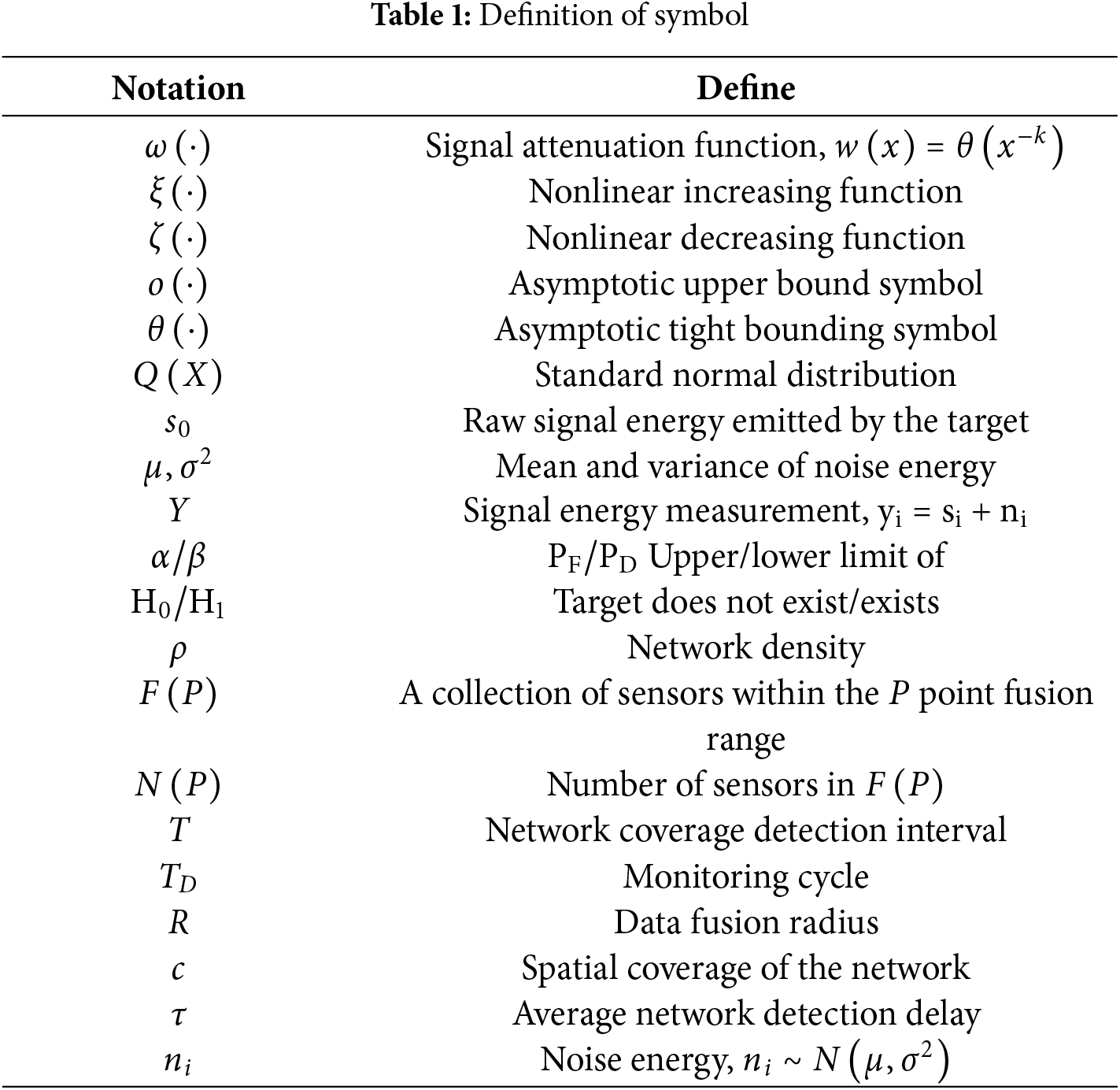
Table 1 explains the symbol applied in this paper.

3.2.2 Definition of Terms

Definition 1. ((α,β)−covered) For a target point P to be detected, if the false alarm rate PF and the detection probability PD(p) satisfy PF≤α, PD(p)≥β, where α∈(0,0.5) and β∈(0.5,1), then the target point P is (α,β)−covered.

Definition 2. (Spatial coverage) The percentage of target points in the target area that are covered by (α,β)−covered.

Definition 3. (α−delay) The α−delay is the average number of detection cycles from the first detection to the target provided that PF is not greater than α.

Definition 4. (Temporal coverage) Time Override is the inverse of α−delay.

Definition 5. (False alarm rate PF) PF is the probability that the sensor determines the presence of a target point when no target point is present.

Definition 6. (Detection rate PD) PD is the probability that a target point is present, and the sensor detects it.

3.3 Derivation of the Fitness Function

3.3.1 Objective 1. Maximize Network Lifecycle

The network lifecycle is an important metric for measuring the merits of a network deployment. The network coverage should at least exceed a given threshold to ensure the proper operation of the wireless sensor network [46]. So, in this paper, the network lifecycle is defined as the time from the initialization of the network to the time when the minimum threshold value of network coverage cannot be met. The network is tested for coverage at every interval of T time, assuming that the network does not satisfy the coverage minimum threshold value when it is detected at the first n time, then the network lifecycle is judged to be over then the network life cycle can be defined as Eq. (5).

LT=∑i=1nTi(5)

3.3.2 Objective 2. Maximize Spatial Coverage

The spatial coverage of the unified deployment network under the stochastic data fusion model, denoted by is c as Eq. (6).

c≅Q(γ(R)−ρπR2ρπR2)(6)

γ(R)=(Q−1(α)σ−Q−1(β)σs2+σ2μs)2(7)

where μs, σs2 are given by Eqs. (12) and (13).

3.3.3 Objective 3. Maximize Temporal Coverage

The temporal coverage of the unified deployment network under the data fusion model, denoted by is τ as in Eq. (8).

τ=1/E[PD](8)

E[PD]=∑Nj=0NPDj⋅fPoi(Nj|ρπR2)(9)

where E[PD] is the average detection probability of any unit detection, Nj obeys the Poisson distribution, i.e., Nj∼Poi(ρπR2), where fPoi(k|λ) is the probability density function of the Poisson distribution Poi(λ). WherefPoi(k|λ)=λκe−λ/k, PDj are defined as Eq. (11).

3.3.4 Objective 4. False Alarm Rate PF Minimize

The false alarm rate is the probability of false detection by the network and reducing the false alarm rate of the network means increasing the confidence of the network’s detection results. Let Fj be the set of sensors in the fusion range in the j unit detection and there are Nj sensors in Fj. When the target is not present, we have Y|H0=∑i∈Fjni∼N(Njμ,Njσ2) where ni the noise energy is experienced by sensor i. This article assumes that the noise ni at each sensor i obeys a normal distribution, i.e., ni∼N(μ,σ2). The false alarm rate for thejth unit detection PFj can be defined as Eq. (10).

PFj=P(Y≥η|H0)=Q(T−NjμNjσ)(10)

3.3.5 Objective 5. Detection Rate PD Maximization

The false alarm rate and the detection rate are independent of each other and increasing the detection rate improves the quality of the network in detecting target points. When the target is present, the sum of energy measurements in the jth unit detection approximately obeys a normal distribution Y|H1=∑i∈Fjsi+∑i∈Fjni∼N(Njμs+Njμ,Njσs2+Njσ2) the jth unit detection rate can be defined as Eq. (11).

PDj=P(Y≥T|H1)≈Q(T−Njμs−NjμNj⋅σs2+σ2)(11)

where μs, σs2 denote the mean and variance, respectively, of si|i∈F(p) for any point P. μs, σs2 given by Eqs. (12) and (13).

μs=2SiR2⋅∫0Rxω(x)ξ(x)ζ(x)dx(12)

σs2=2Si2R2⋅∫0Rxω2(x)ξ2(x)ζ2(x)dx−μs2(13)

3.4 Problem Description

As mentioned above, under the constraints of complete coverage of the monitoring area and network connectivity, this article investigates the SDFWSN deployment problem by jointly optimizing the five objectives of the network lifecycle, spatiotemporal coverage, false alarm rate, and detection rate. In summary, the SDFWSN deployment problem can be formulated as follows (Eq. (14)):

{max(LT),min(PFj),max(PDj),max(c),max(τ)}s.t.C(GSDFWSN)=1(14)

where C(GSDFWSN)=1 indicates that the network satisfies the connectivity condition.

4  Proposed EMODMOA Algorithm Design Process and Method

This section describes algorithms to solve the problem of sensor deployment in SDFWSN. Considering that Eq. (14) in which the multi-objective optimization problem is a non-convex, discontinuous, multi-modal, and NP-hard problem, this article proposes EMODMOA to solve it. In this section, firstly, the DMOA algorithm is briefly described, secondly, improvement strategies for the algorithm are presented, and finally, EMODMOA is introduced in detail, including the initialization of the algorithm, the iterative process, and the strategy of sub-generation generation. Based on this, the optimal deployment method of SDFWSN based on EMODMOA is further proposed. And the analysis of EMODMOA time complexity is given.

4.1 DMOA

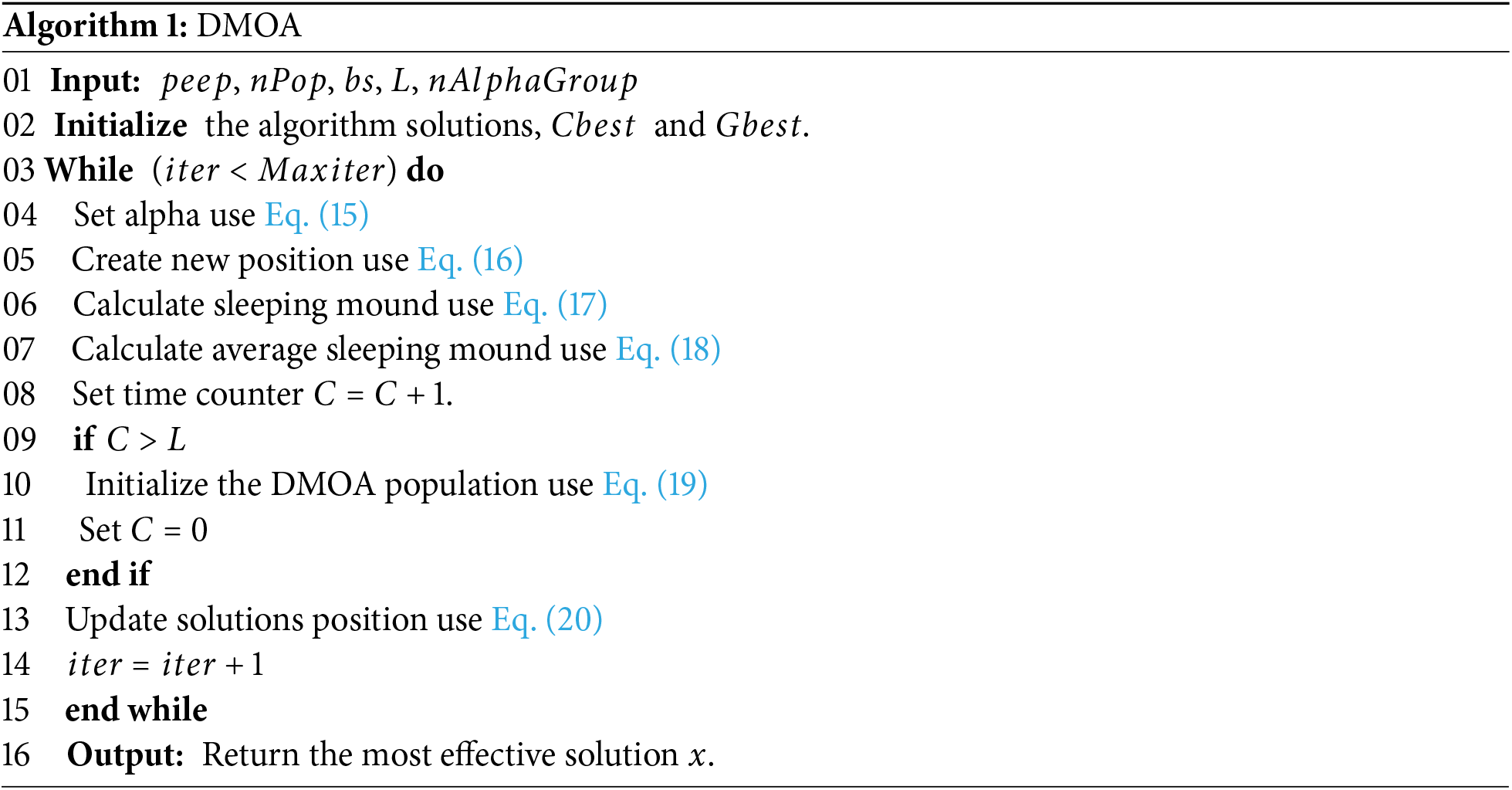
DMOA is a population intelligence optimization algorithm proposed in 2022 by Agushaka et al. DMOA is inspired by the semi-nomadic and compensatory adaptive behavior of dwarf mongoose populations. The algorithm has a strong global search capability. The algorithm is divided into four main phases, searching for food, searching for mounds (exploitation phase), babysitter exchange, and choosing mounds (exploration phase) [13].

(1) Food search phase:

The algorithm divides the mongoose into an alpha group (scouting group) and a babysitter group based on their compensatory adaptive behavior, and the alpha group searches for the location of the optimal food during the food search phase. The alpha group leader is selected according to Eq. (15) and the individual position update formula is given by Eq. (16).

α=fiti∑i=1nfiti(15)

Xi+1=Xi+phi∗peep(16)

where phi is a uniformly distributed random number [−1, 1] and peep is the sound made by the alpha female.

(2) Mounds search phase:

The scouting group is responsible for finding the sleep mounds, and evaluation formula for individual sleep mounds as Eq. (17). Evaluation formulas for population sleep mounds are given by Eq. (18).

smi=(fiti+1−fiti)max{fiti+1,fiti}(17)

ϕ=∑i=1nsmin(18)

where fiti+1, fiti denote the fitness values of the mongoose’s new position and the original position respectively.

(3) Babysitter exchange phase:

Once the babysitter swap conditions are met, the babysitter group and alpha (scout) group will swap identities. Initialize the mongoose’s new location as Eq. (19).

xi,j=unifrnd(VarMin,VarMax,VarSize)(19)

(4) Mounds choose phase:

During this phase, an individual chooses an optimal sleep mound to perch on, and the individual position equation is as follows Eq. (20). Where M is given by Eq. (21), CF is the adaptive operator and the formula is as Eq. (22).

Xi+1={Xi−CF∗phi∗rand[Xi−M],ifϕi+1>ϕiXi+CF∗phi∗rand[Xi−M],otherwise(20)

M=∑i=1nXi∗smiXi(21)

CF=(1−iterMaXiter)(2iterMaxiter)(22)

The DMOA pseudo-code is shown in Algorithm 1.

4.2 EDMOA

This subsection describes the proposed EDMOA algorithm, and the new algorithm focuses on the improvement of the original algorithm for the shortcomings that it is easy to fall into local optimal solutions, slow convergence, and imbalance between exploration and exploitation.

Encircling and Hunting Strategy

Because the dwarf mongoose has the characteristic of rounding up foraging, an encircling and hunting strategy is proposed based on the biological characteristics of the dwarf mongoose to better simulate the biological behavior of the dwarf mongoose. This strategy draws inspiration from the grey wolf optimization algorithm. First, three optimal markets are selected as Pα, Pβ and Pδ. Distances between individual mongoose and among them are computed as per Eqs. (23)–(25).

dα=|c1⋅Pα−xi|(23)

dβ=|c2⋅Pβ−xi|(24)

dδ=|c3⋅Pδ−xi|(25)

where c1, c2 and c3 is random numbers within the range of [0, 1] are used to randomly select three non-optimal mongoose, P1, P2 and P3 from the remaining n−3 individuals. These selected mongooses undergo computations as per Eqs. (26)–(28).

P1=ϕ⋅Pr1−r⋅(dα)(26)

P2=ϕ⋅Pr2−r⋅(dβ)(27)

P3=ϕ⋅Pr3−r⋅(dδ)(28)

where r1, r2 and r3 is random numbers within the range of [0, 1], r is random numbers within the range of [−1, 1], ϕ=e−0.05∗t.

The mongoose individuals are updated according to Eq. (29).

xi+1=P1+P2+P33(29)

The pseudo-code of the EDMOA algorithm is as follows (Algorithm 2):

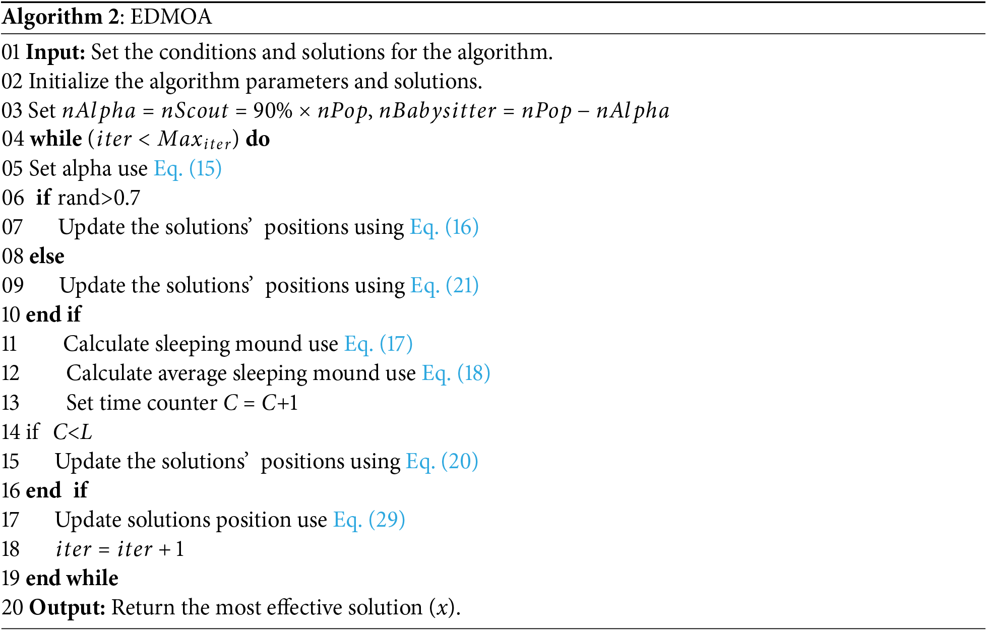
EDMOA update flowchart is shown in Fig. 1.

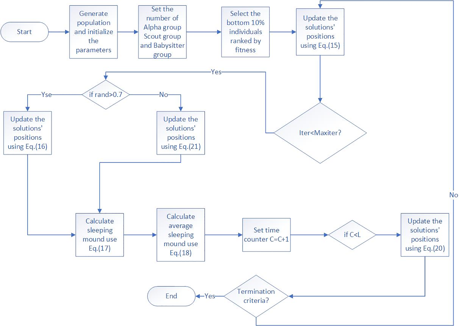
Figure 1: Flowchart of EDMOA

4.3 EMODMOA

The design of EMODMOA refers to the algorithm framework of NSGAIII, but in the selection of reference points, the classification algorithm KNN is used to classify individuals close to the reference points, select individuals in small categories, ensure the diversity of the population, and reduce the complexity of the algorithm. The pseudo-code of EMODMOA is shown in Algorithm 3, and the algorithm flowchart is as follows:

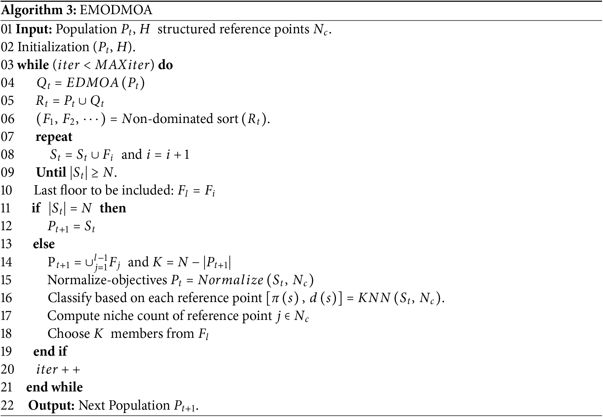
Algorithm 3 is the pseudo-code of EMODMOA, in EMODMOA Pt is the parent of tth generation of size N and its generated child is Qt which is also of size N. Combining the child and the parent generates Rt of size 2N and selects N individuals from it. To implement this selection process, Rt is first divided into multiple non-dominated layers (F1,F2,⋯) by non-dominated ordering. The members of the populations in the non-dominated stratum rank 1 to l are put into St in order, and if |St|=N, the following operation is not necessary, and Pt+1=St directly. If |St|>N, then a part of the next generation is solved as Pt+1=∪j=1l−1Fj, and the remaining part (K=N−|Pt+1|) is chosen from Fl. The selection principle is to classify according to the KNN algorithm, selecting individuals that are far from the reference point, thereby maintaining the diversity of the solution.

The SDFWSN is deployed on a 4000 m × 4000 m static node grid. The false alarm rate of each node is lower than 0.05 detection rate is higher than 0.95. The optimization process for the deployment of a stochastic fused wireless sensor network consisting of 220 nodes using EMODMOA is as follows:

Step 1. Initialize the parent population Pt and the reference point Nc. Pt is denoted as follows:

Pt=[X1,X2,,XN]T(30)

where Xi=[x,y,Rc,n] is the ith individual in the population Pt representing a feasible deployment of a wireless sensor network. n is the number of sensors in the network, x and y are n dimensional column vectors, and Rc is the connectivity radius of the network.

Step 2. Generate child population Qt by updating iteration of parent population Pt using EDMOA and merge the parent and child populations into Rt.

Step 3. Generate a Pareto frontier by the non-dominated ordering of Rt.

Step 4. Starting from the first Pareto frontier select individuals to population St until the number of St is greater than or equal to the initial population size.

Step 5. Use KNN to select individuals in the selected last Pareto frontier to join the population St until the number of St is equal to the initial population size. The population St is the deployment scheme of SDFWSN.

The EMODMOA flowchart is shown in Fig. 2.

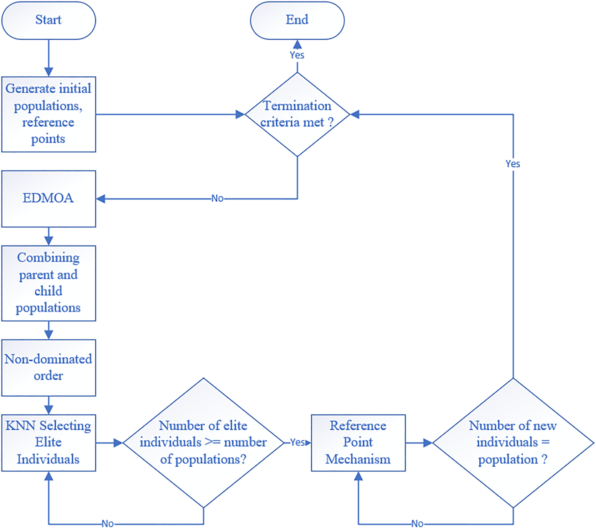
Figure 2: Flowchart of EMODMOA

5  Function Performance Testing

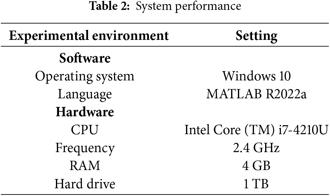
In this section, the performance of the proposed EMODMOA is examined using the CEC2020 multi-objective multi-modal optimization benchmark function. This benchmark function contains 24 different types of test functions for convex and concave, linear and nonlinear. Each function corresponds to objective space and decision space with optimal Pareto front (PF) and multiple local or global optimal PS sets. The performance metrics we use in the objective space are the hypervolume inverse (rHV) [47] and the Inverted Generational Distance (IGDF) [48]; in the decision space we use the inverse of the Pareto Strength Pareto (rPSP) [49] and the Inverted Generational Distance (IGDX) [48] as performance metrics. The system configuration of this experimental platform is shown in Table 2.

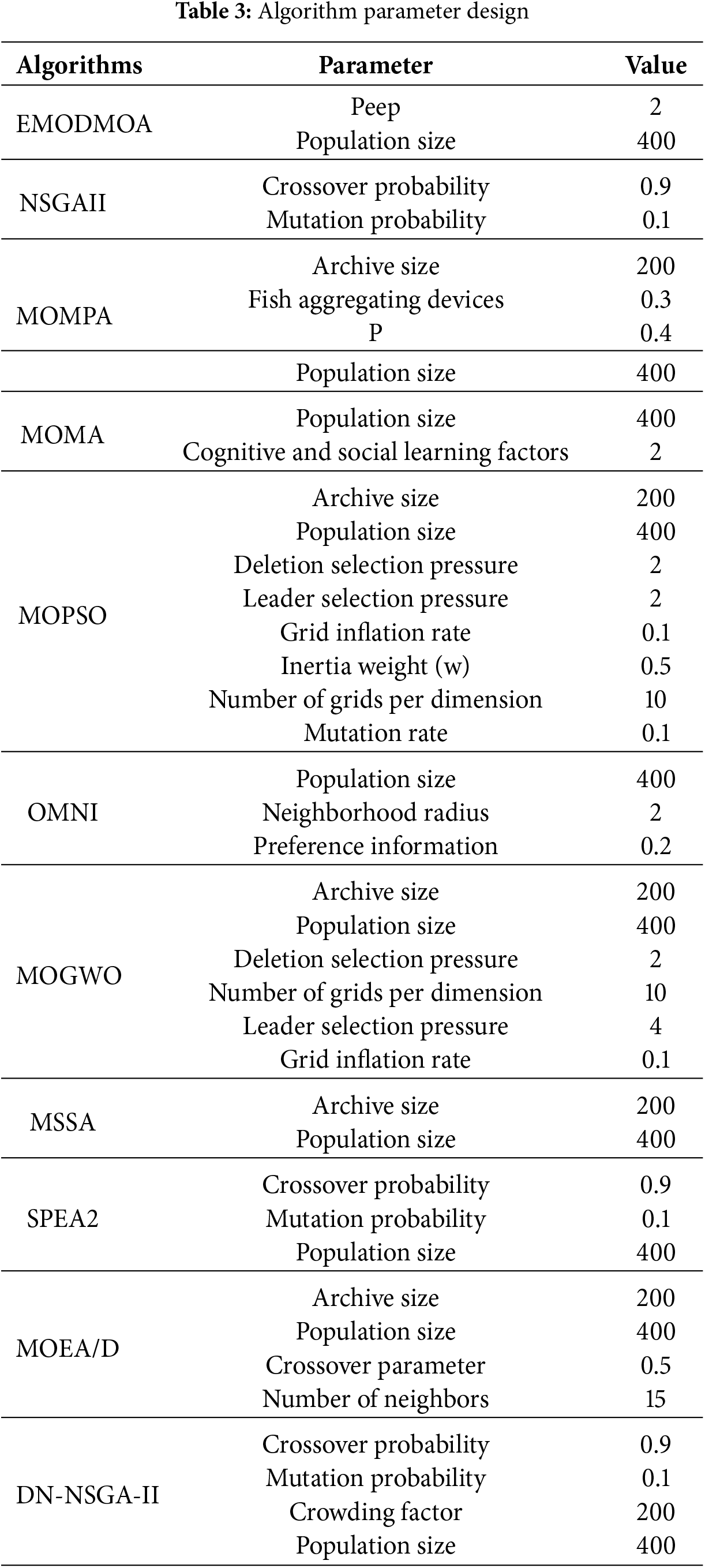
The proposed algorithms are compared with 10 mainstream multi-objective algorithms including Multiple Objective Particle Swarm Optimization (MOPSO), Multi-objective Marine Predators Algorithm (MOMPA), Multi-Objective Evolutionary Algorithm based on Decomposition (MOEA/D), Non-dominated Sorting Genetic Algorithm II (NSGAII), Strength Pareto Evolutionary Algorithm 2 (SPEA2), Nominal Diameter Non-dominated Sorting Genetic Algorithm II (DN-NSGA-II), Multi-Strategy Salp Swarm Algorithm (MSSA), Multi-Objective Grey Wolf Optimizer (MOGWO), Multi-Objective Mayfly Algorithm (MOMA) and optimal mini niche Non-dominated Sorting Genetic Algorithm (OMNI). The parameters of each algorithm are set in Table 3. Each algorithm was run independently 21 times with 100 iterations and the mean and variance values obtained from each function test were recorded. “+”, “=” and “−” indicate that EMODMOA performs better than, equal to, and worse than the other algorithms, respectively.

Tables 4–7 show mean, and standard deviation results obtained by the algorithms on different performance metrics, with each row in black font indicating the optimal result for the corresponding test function. The last row of the table records the performance comparison between EMODMOA and the other algorithms on each test problem.

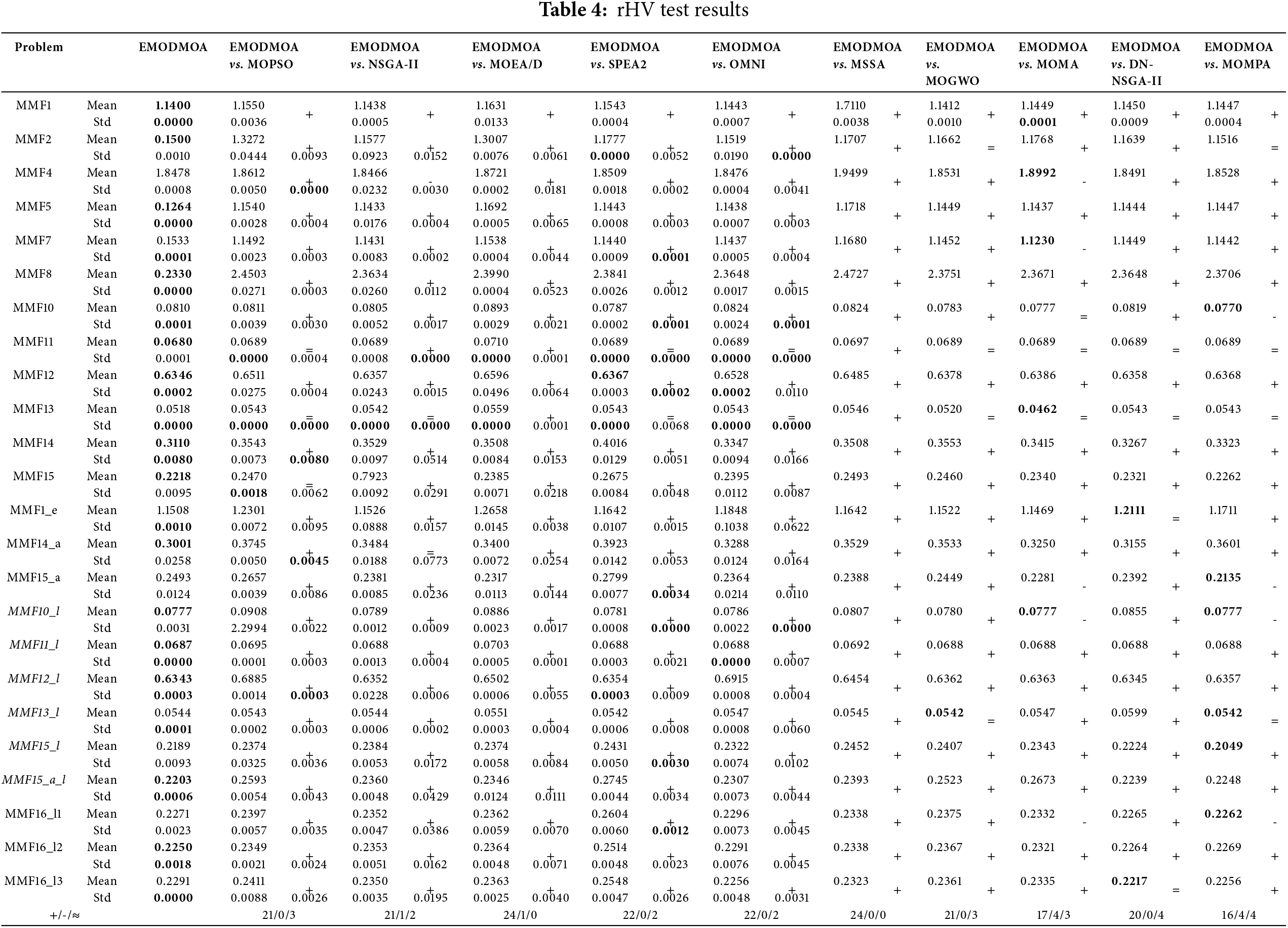
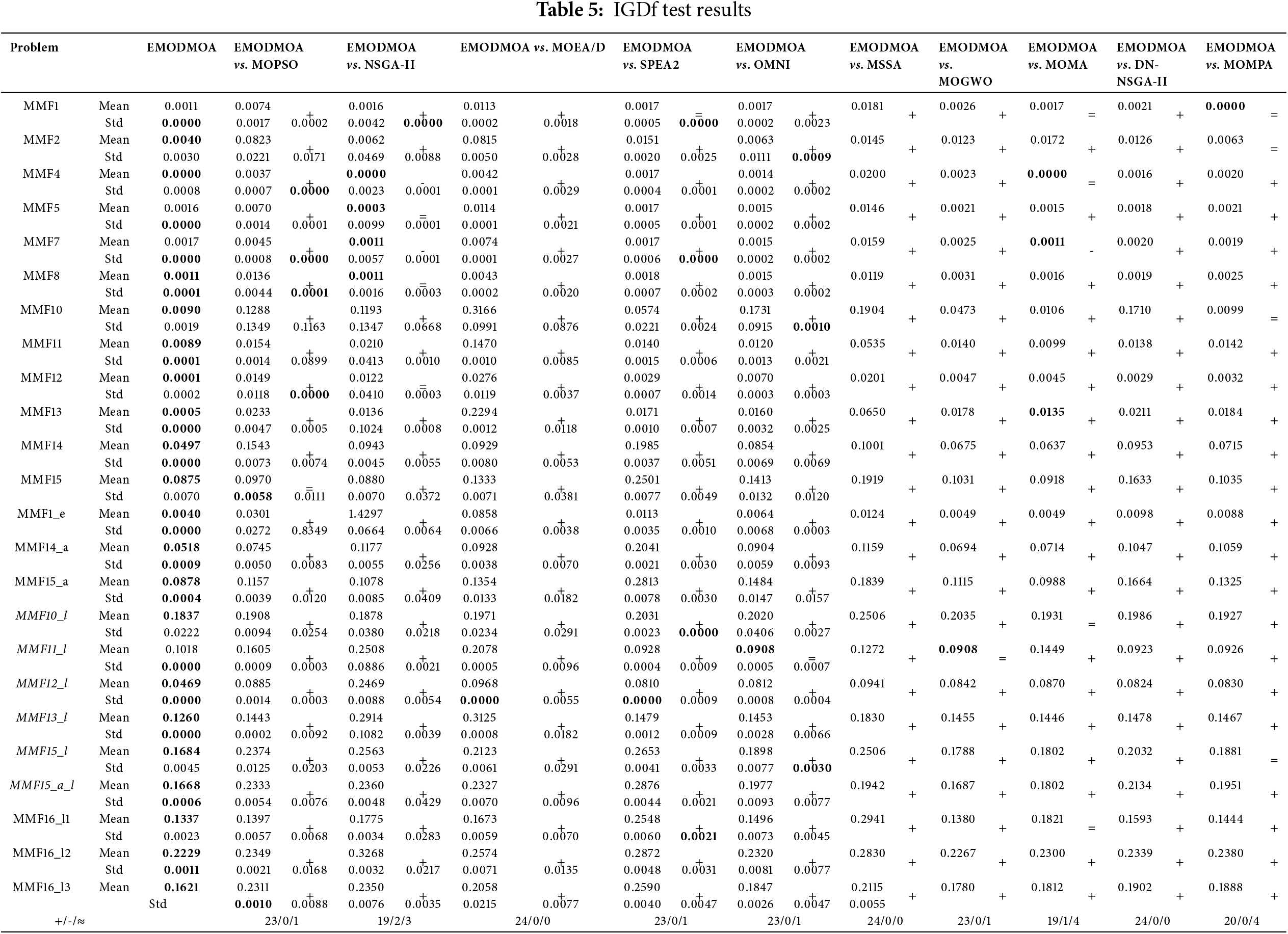
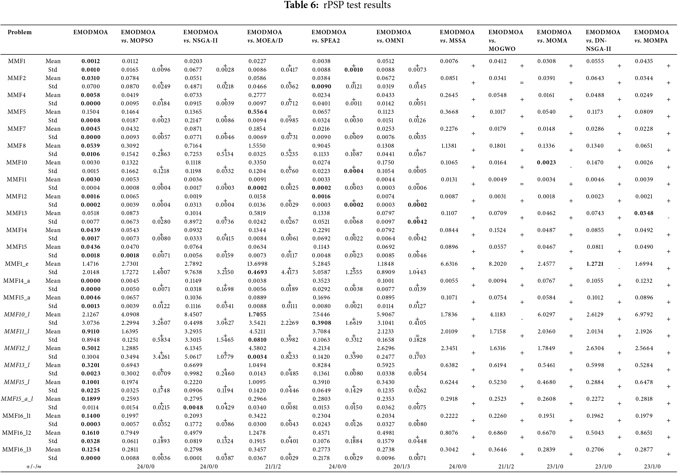
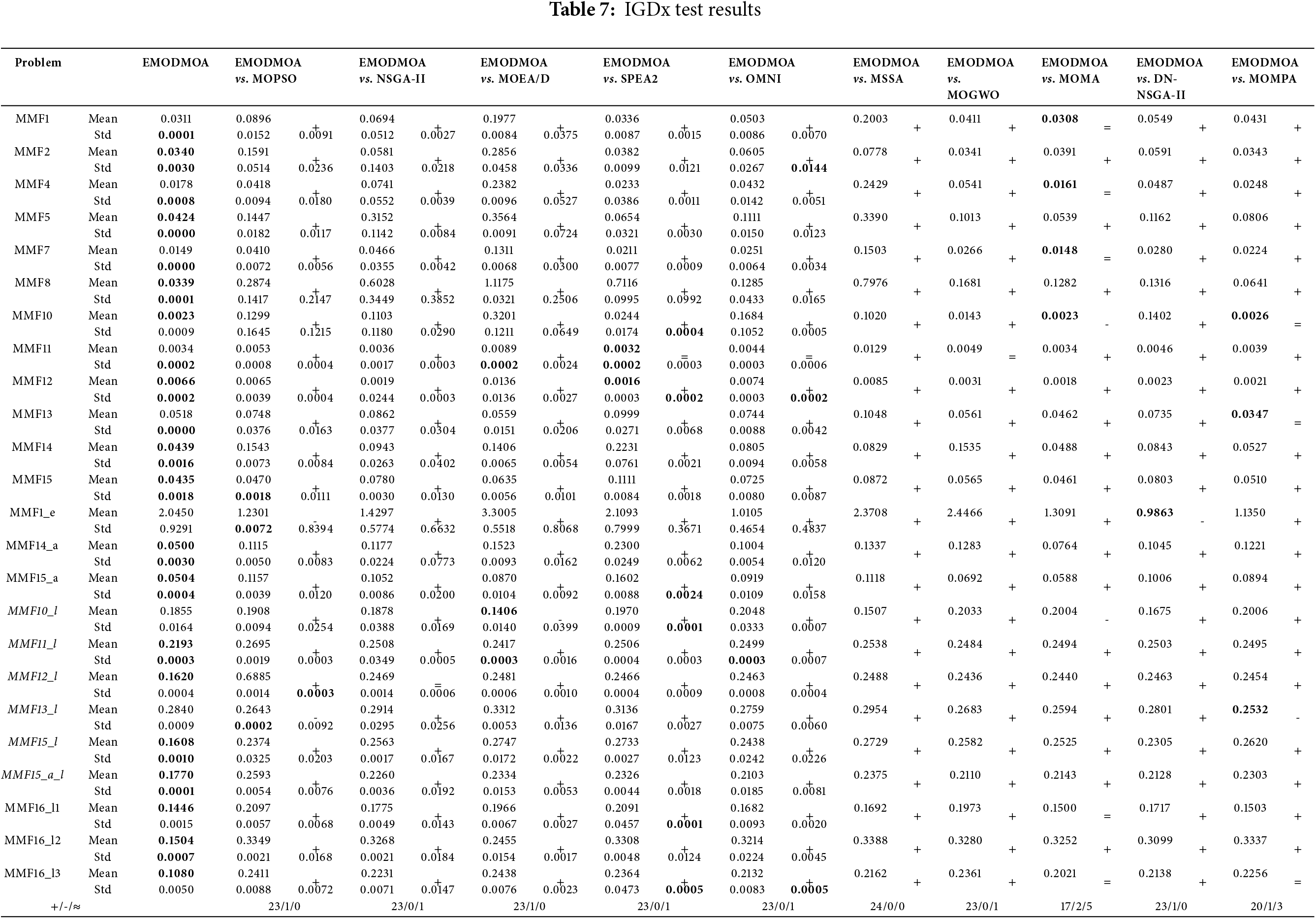
Table 4 provides statistics on the rHV obtained by different algorithms. The smaller the rHV, the wider the coverage of the multidimensional objective space of the resulting Pareto front. As can be seen from the table, EMODMOA obtained the minimum value among the 15 functions, which is much better than the other algorithms. Although EMODMOA failed to obtain the minimum value in 9 functions, the mean and standard deviation of the rHV index of these functions are still ranked first. This is because EDMOA very well simulates the biological characteristics of the dwarf mongoose, making the algorithm have strong global search capabilities, not disturbed by local optima, and can maximize the number of non-dominated solutions, thus greatly improving the convergence and diversity of the algorithm.

Table 5 shows the IGDf results obtained by each algorithm. On IGDf, EMODMOA achieves the minimum in 20 functions and its performance is far beyond the other algorithms. The results obtained in Multi-objective Multimodal test function1 (MMF1), MMF5, MMF7, and MMF11_l are also very competitive although no minimum is achieved. This proves once again that EMODMOA has strong search capability and convergence performance, which matches the rHV results shown in Table 4.

The rPSP is used to measure the uniformity and compactness of the solutions obtained by the measurement algorithm in the Pareto front. The rPSP values obtained by different algorithms are recorded in Table 6. As can be seen from the table, among the 19 test functions, EMODMOA has the smallest value and ranks first among all algorithms. In functions MMF5, MMF10, MMF13, and MMF1_e, EMODMOA did not obtain the smallest value, but the optimization results were also very competitive among all algorithms, and the number of minimum values obtained by other algorithms was far less than that of EMODMOA. The comparison of rPSP values shows that EMODMOA can obtain a Pareto front with a uniform distribution and compact arrangement, which proves that EMODMOA has a strong global search capability. This is due to the improvement of the original DMOA algorithm, which combines the obtained solution with the best solution of the previous generation and uses KNN to select reference points to retain the best solution. Therefore, EMODMOA can find multiple optimal solutions for multimodal problems, demonstrating excellent search capabilities.

Table 7 gives the statistics of the performance metric IGDx. In Table 7, EMODMOA’s results for IGDx are better than the other algorithms. Minimum values were obtained for 16 functions and good results were obtained although no minimum values were obtained for the remaining functions. It shows that EMODMOA is very good at searching the decision space and IGDx measures the convergence between the PS obtained by the algorithm and the true PS. Combined with the results of rPSP in Table 6, it proves that EMODMOA is better than other algorithms in its global search ability.

Overall, the overall performance of EMODMOA in CEC2020 is excellent. EMODMOA can get closer to the global optimal solution and more diverse Pareto frontiers. This fully reflects its superior search performance and convergence and proves that we can lead the EMODMOA algorithm to solve real multi-objective problems.

6  Experimental Results and Discussion

In this study, the EMODMOA algorithm is used to solve the SDFWSN deployment, which is deployed on a static node grid of 4000 m × 4000 m. The false alarm rate of each node is lower than 0.05, detection rate is higher than 0.95. The SDFWSN consists of 220 sensor nodes. The proposed EMODMOA algorithm is compared parametrically with the existing multi-objective algorithms NSGAII, MOPSO, MOEA_D, and MOGWO in terms of the network lifecycle, spatial coverage, temporal coverage, false alarm rate, and detection rate. And to better evaluate the performance of the proposed algorithms, this article adopts the widely used evaluation metrics in multi-objective optimization algorithms [50], hyper volume (HV), Delta and non-dominant solution (NDS) metrics are evaluated for the multi-objective algorithm. Table 8 lists the experimental settings and their values. Table 9 shows the parameter settings of the various multi-objective algorithms compared.

6.1 Basic Experiment

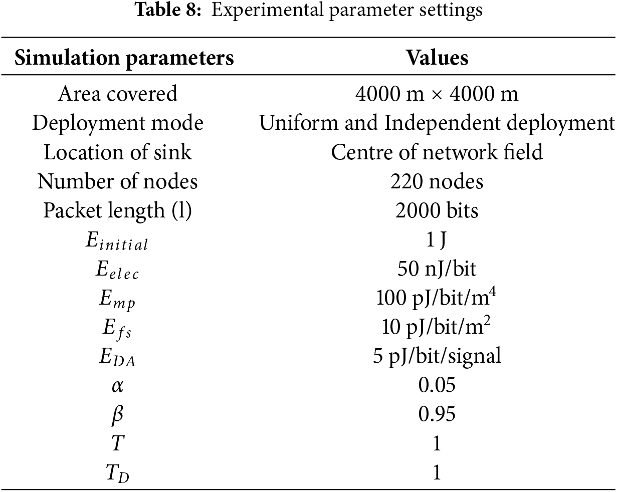
The HV index evaluates the convergence and diversity of the solution set by comparing the hypercube between the solution set and the reference point. The HV index is positive. In multi-objective optimization, the larger the hypercube occupied by the solution set, the better the performance of the solution set, indicating that the algorithm has found a better solution in the objective space. The Delta index is a commonly used evaluation index that can help determine the diversity and homogeneity of the solution set generated by the optimization algorithm. It measures the degree of dispersion of the solutions within the solution set and provides information about the structure of the solution set. The closer the Delta metric is to 1, the better the diversity and homogeneity of the solution set; the closer it is to 0, the worse the diversity and homogeneity of the solution set. NDS is the number of optimal solution sets obtained by the algorithm, which intuitively reflects the algorithm’s ability to find the best solution. In this paper, the HV, Delta, and NDS values of NSGAII, MOPSO, MOEA_D, and MOGWO are compared with those of the EMODMOA algorithm. The results are shown in Figs. 3–5. The results show that the super-volume values obtained by the EMODMOA algorithm are higher than those of the other algorithms under different parameter settings, which indicates that the EMODMOA algorithm has strong convergence. Moreover, the Delta and NDS values of EMODMOA are higher than those of the other algorithms, which indicates that EMODMOA can find a Pareto frontier with more diversity and richness, and thus provide decision-makers with more choices.

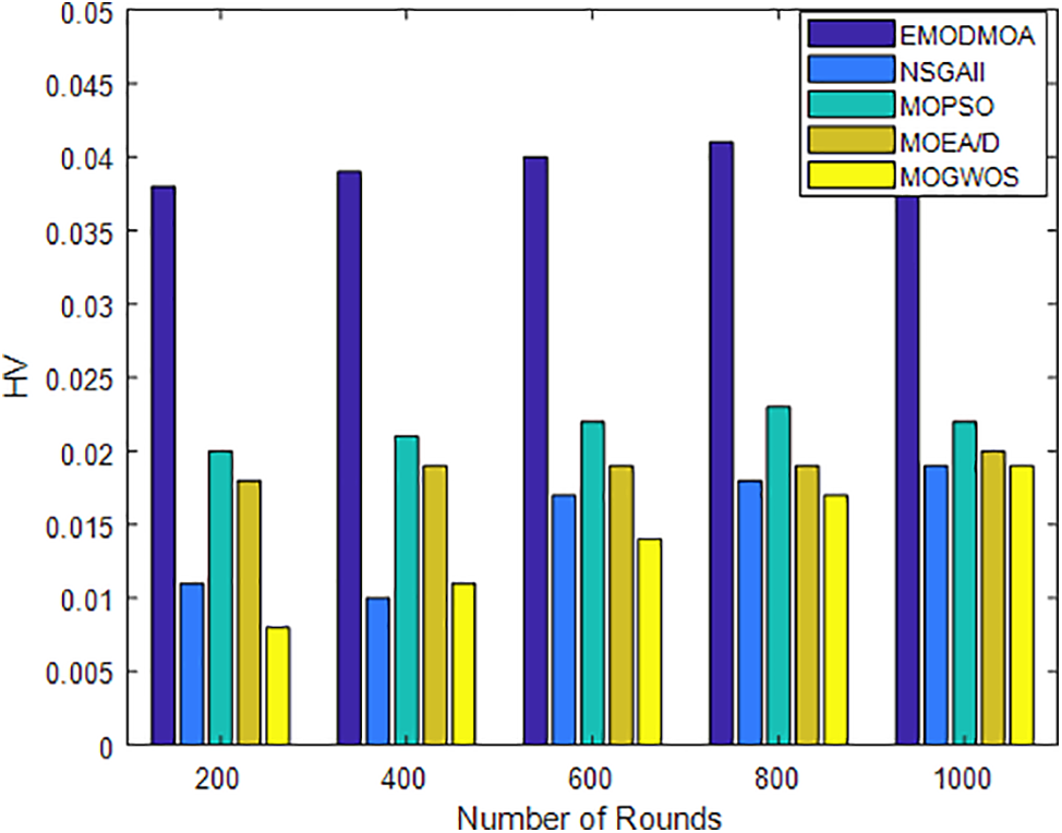
Figure 3: HV vs. Number of iterations

Figure 4: NDS vs. Number of iterations

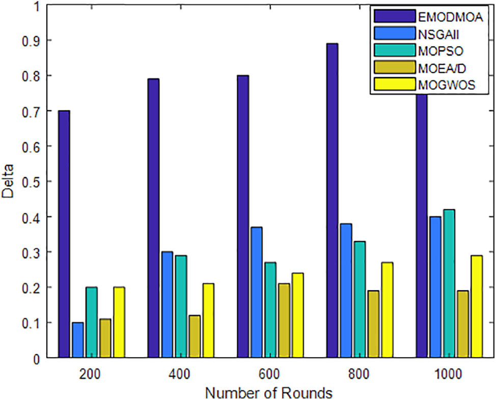
Figure 5: Delta vs. Number of iterations

Fig. 6 shows the network life cycle as the number of iterations increases. It can be seen from the figure that the network life cycle is extended with optimization. Comparing the EMODMOA algorithm with algorithms such as NSGAII, MOPSO, MOEA/D, and MOGWO, our proposed algorithm obtains the maximum network life cycle after 500 iterations. As can be seen from the direction of the broken line in the figure, EMODMOA can steadily improve the network life cycle, and it has the highest stability among all algorithms.

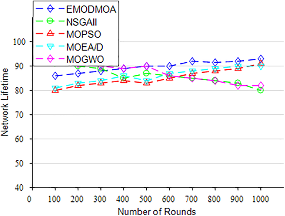
Figure 6: Network lifecycle vs. Number of iterations

The analysis of the spatial coverage of the network is given in Fig. 7, which improves with the number of iterations. A comparison of the EMODMOA algorithm with NSGAII, MOPSO, MOEA/D, and MOGWO reveals that our proposed algorithm gives the optimal spatial coverage of the network at the later stage of iteration. This is due to the scientific improvement of our algorithm and shows that our proposed algorithm is highly competitive among many multi-objective optimization algorithms.

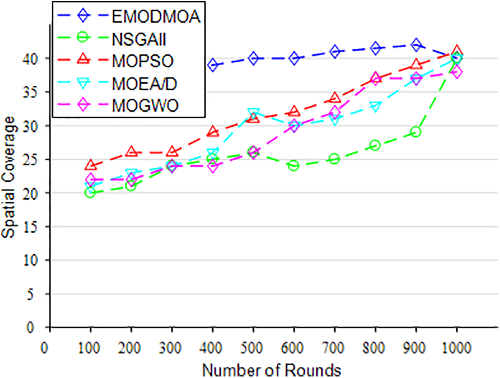
Figure 7: Spatial coverage vs. Number of iterations

Fig. 8 gives an analysis of the network time coverage, which is optimized with the increase of the number of iterations. Comparing EMODMOA with NSGAII, MOPSO, MOEA/D, and MOGWO, it is found that the final iteration result of our proposed algorithm has the best time coverage. Compared with the broken lines obtained by other algorithms, the optimized broken lines obtained by our algorithm tend to grow steadily, which indicates that our proposed algorithm has strong stability.

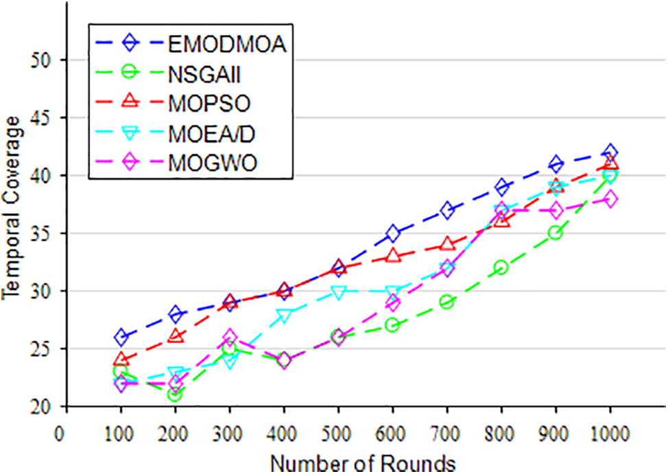
Figure 8: Temporal coverage vs. Number of iterations

Figs. 9 and 10 show the detection rate and false alarm rate of the network, respectively. The detection rate indicates the probability that the network correctly detects the target, while the false alarm rate indicates the probability that the network transmits information about the existence of a target when there is no target. Therefore, as the number of iterations increases, the algorithm should improve the detection rate of the network while reducing the false alarm rate. Observing Fig. 9, it can be found that all algorithms have optimized the detection rate, and the MOGWO algorithm has achieved the optimal detection rate. Although the algorithm proposed in this paper has not achieved the optimal detection rate, the detection rate obtained is not much different from the optimal detection rate. In addition, compared with Fig. 10, it can be found that although the MOGWO algorithm achieves the optimal detection rate, the optimization effect on the false alarm rate is not ideal. In contrast, EMODMOA, MOPSO, and MOEA/D improve the detection rate while reducing the false alarm rate. EMODMOA achieves a good detection rate and an optimal false alarm rate, thereby improving network performance.

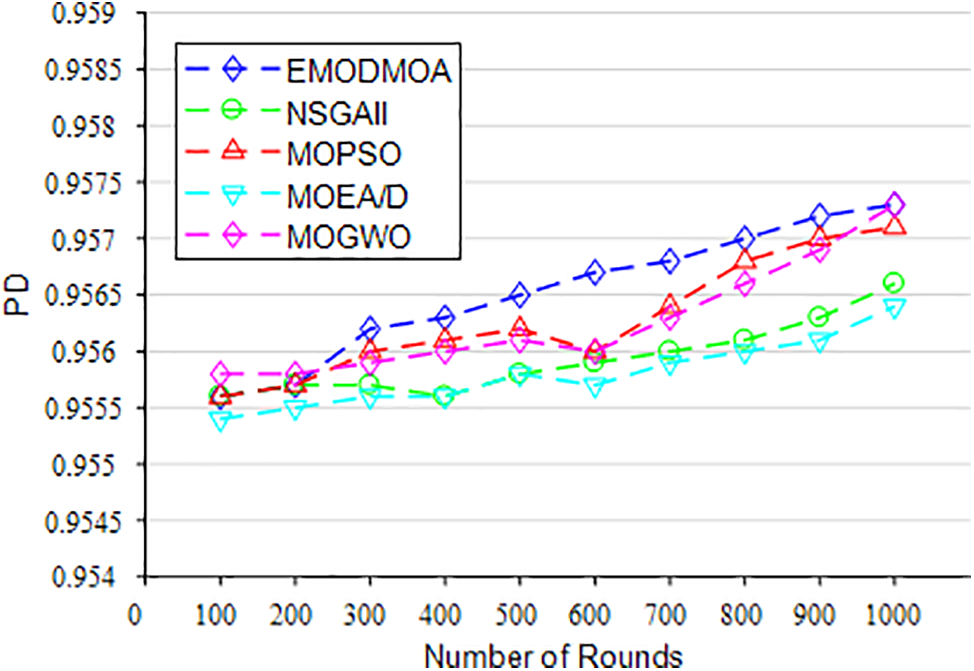
Figure 9: Detection rate vs. Number of iterations

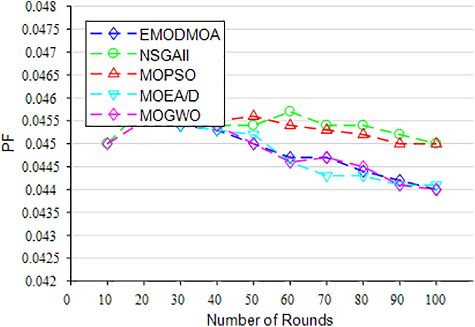
Figure 10: False alarm rate vs. Number of iterations

Fig. 11 shows the deployment of the sensors optimized by the EMODMOA algorithm, and after the optimized deployment, the sensor nodes can cover almost all the target areas. Our algorithm can optimize the deployment of wireless sensors very well. Improve the spatial coverage of the network.

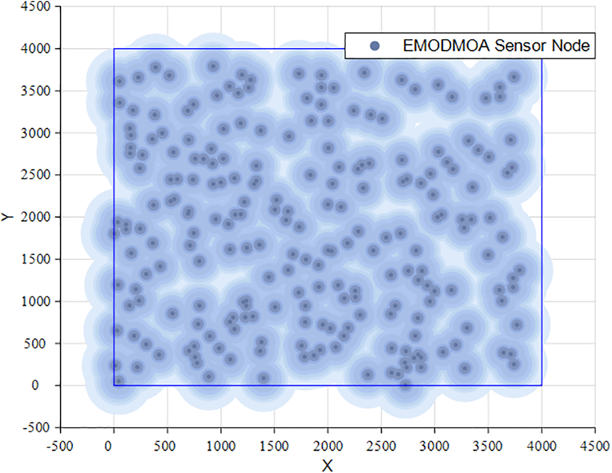
Figure 11: Optimization by EMODMOA

Fig. 12 shows the data fusion graph of SDFWSN, the red circle indicates the sensors that perform data fusion, and the optimized nodes are evenly distributed, and a certain number of sensors are distributed in each data fusion range, which ensures the quality of network transmission. Since the sensors use stochastic sensing, the quality of sensing decreases as the distance between the target node and the sensor increases, the shades of blue in the graph represent the quality of the target area covered by the sensors, i.e., the PD value of the target area, which represents the accuracy degree of the network in detecting the target, and it can be seen that most of the target areas are covered by a higher quality to ensure the accuracy of the network monitoring. This provides a good guarantee for network QoS.

Figure 12: Sensor data fusion of EMODMOA

Figs. 13–16 represent the data fusion maps after optimization with the MOEA/D, MOGWO, MOPSO, and NSGAII algorithms, comparing Figs. 13–16 with Fig. 12, the superiority of network nodes deployed using EMODMOA can be found. First, the nodes of the network optimized using other algorithms are unevenly distributed, and all of them have different degrees of coverage gaps, which will affect the quality of the network. Second, the uneven distribution of the number of sensors within the fusion range leads to poor detection accuracy, i.e., the network cannot provide accurate detection results, which directly affects the QoS of the network. In summary, it can be found that the deployment of the network optimized by EMODMOA is much better than the deployment of network nodes optimized using the other four algorithms, which can be seen in the algorithms of the superiority of the deployment of the network nodes.

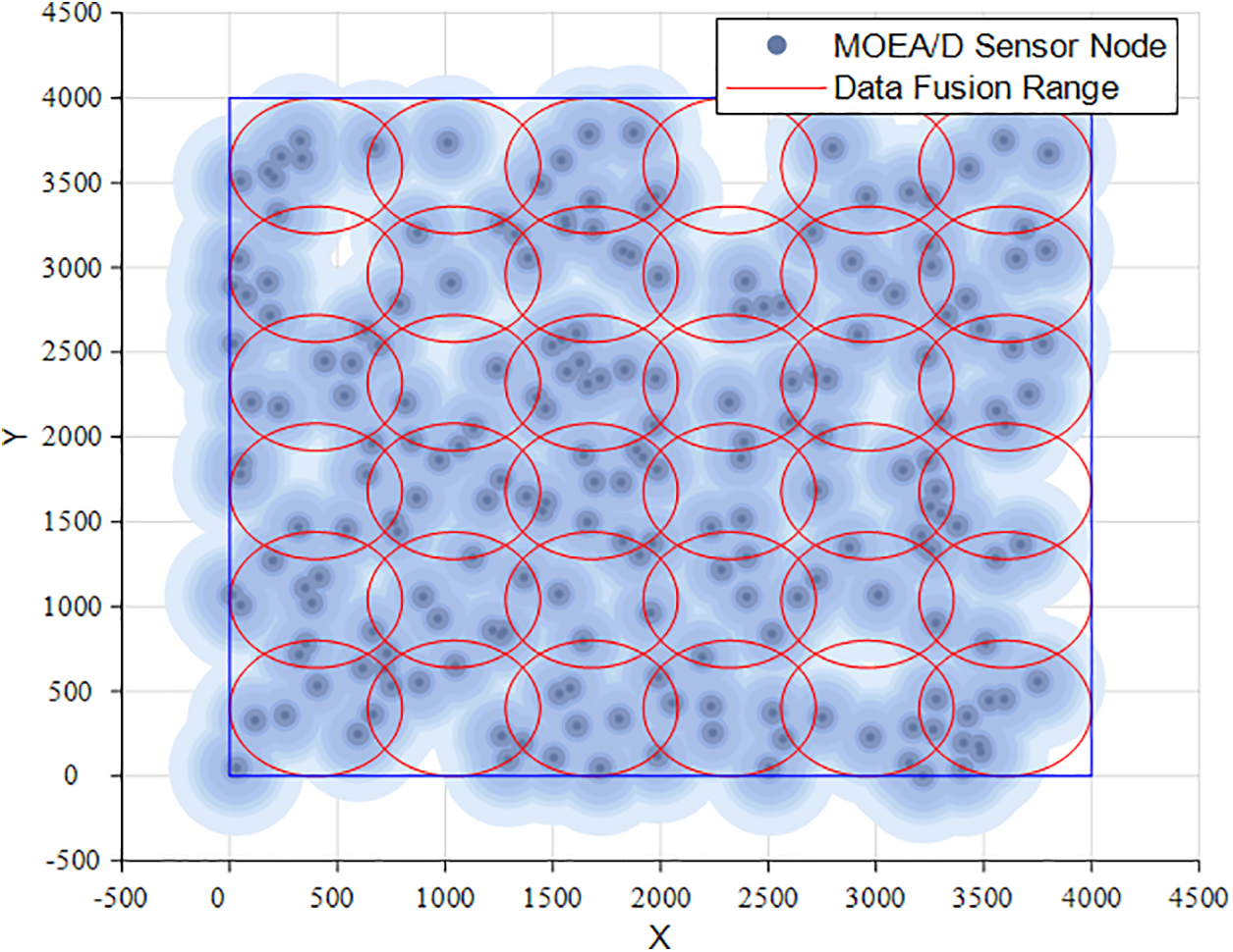
Figure 13: Sensor data fusion of MOEA/D

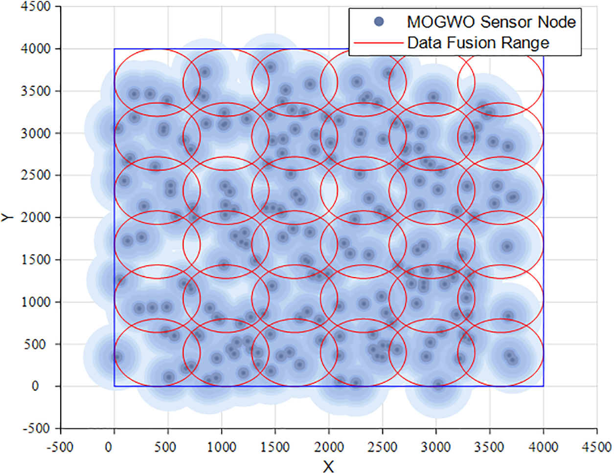
Figure 14: Sensor data fusion diagram of MOGWO

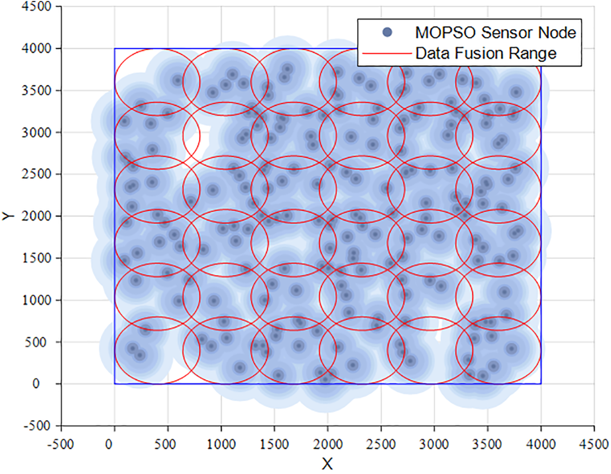
Figure 15: Sensor data fusion diagram of MOPSO

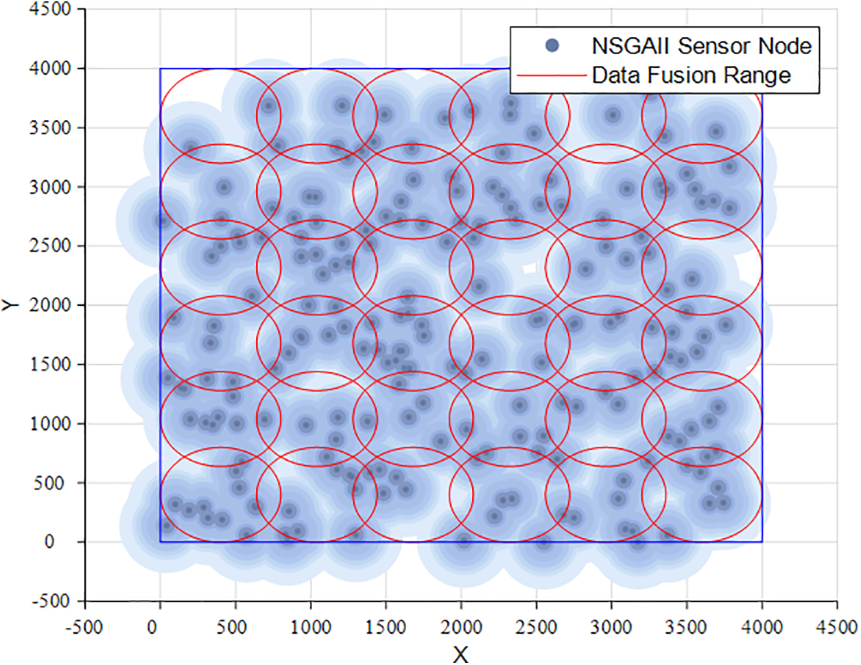
Figure 16: Sensor data fusion diagram of NSGAII

In the simulation experiment, 220 wireless sensors are required to cover an area of 16 × 106 m2. After the experimental deployment, it is calculated that the coverage areas of EMODMOA, MOPSO, MOGWO, MOEA/D, and NSGAII are 15.1 × 106 m2, 13.1 × 106 m2, 12.2 × 106 m2, MOEA/D covers an area of 12.9 × 106 m2, and NSGAII covers an area of 12.4 × 106 m2. The calculation time for each algorithm is shown in Fig. 17 below. Within the allowable time frame, EMODMOA achieved the optimal coverage.

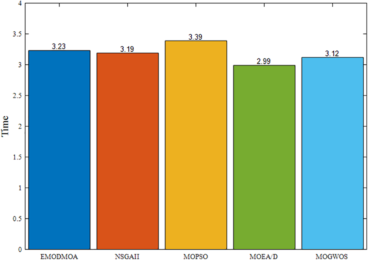
Figure 17: Algorithm running time

6.2 Use Case

To enhance the credibility of the algorithm, four different use cases are designed for verification. The deployment of many nodes and a small number of nodes in a small area, i.e., 1000 m × 1000 m, is discussed, as is the deployment of many nodes and a small number of nodes in a large area, i.e., 5000 × 5000.

Case 1: 300 nodes are deployed within a 1000 m × 1000 m range, and the network coverage is as Fig. 18.

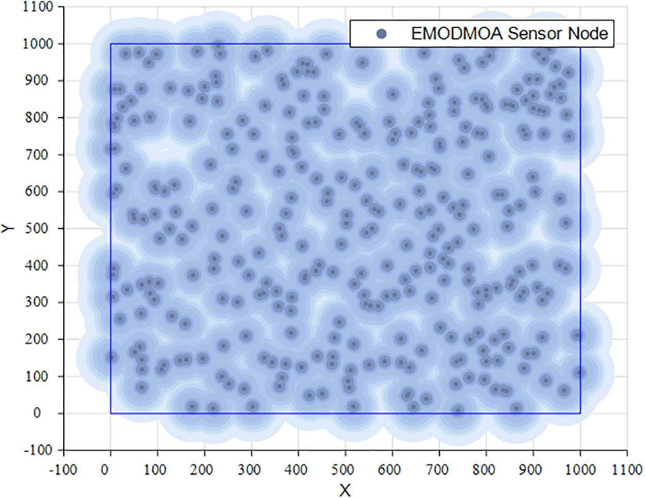
Figure 18: 1000 m × 1000 m range and 300 nodes

Case 2: 100 nodes are deployed within a 1000 m × 1000 m range, and the network coverage is as Fig. 19.

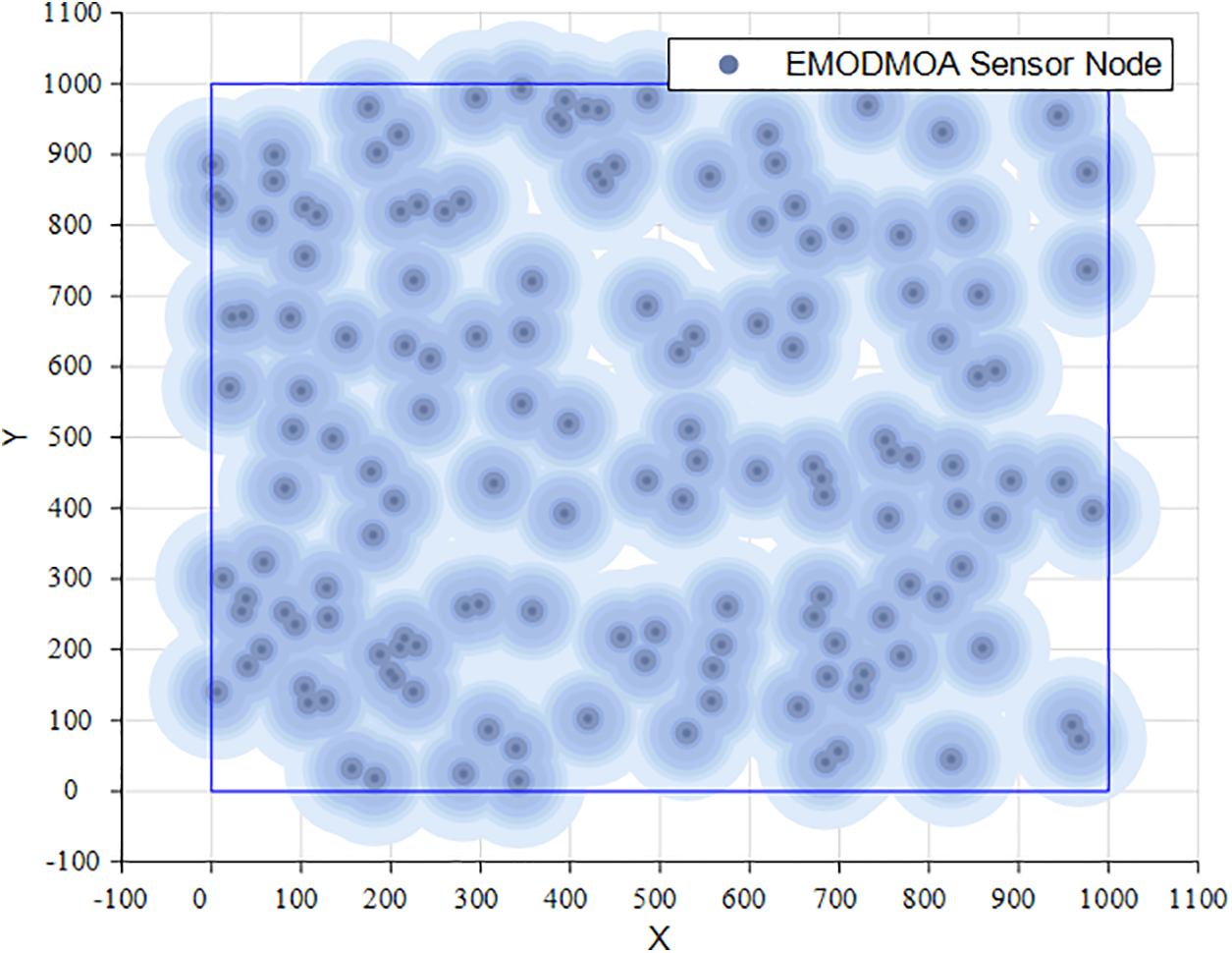
Figure 19: 1000 m × 1000 m range and 100 nodes

Case 3: 300 nodes are deployed within an area of 5000 m × 5000 m, and the network coverage is as Fig. 20.

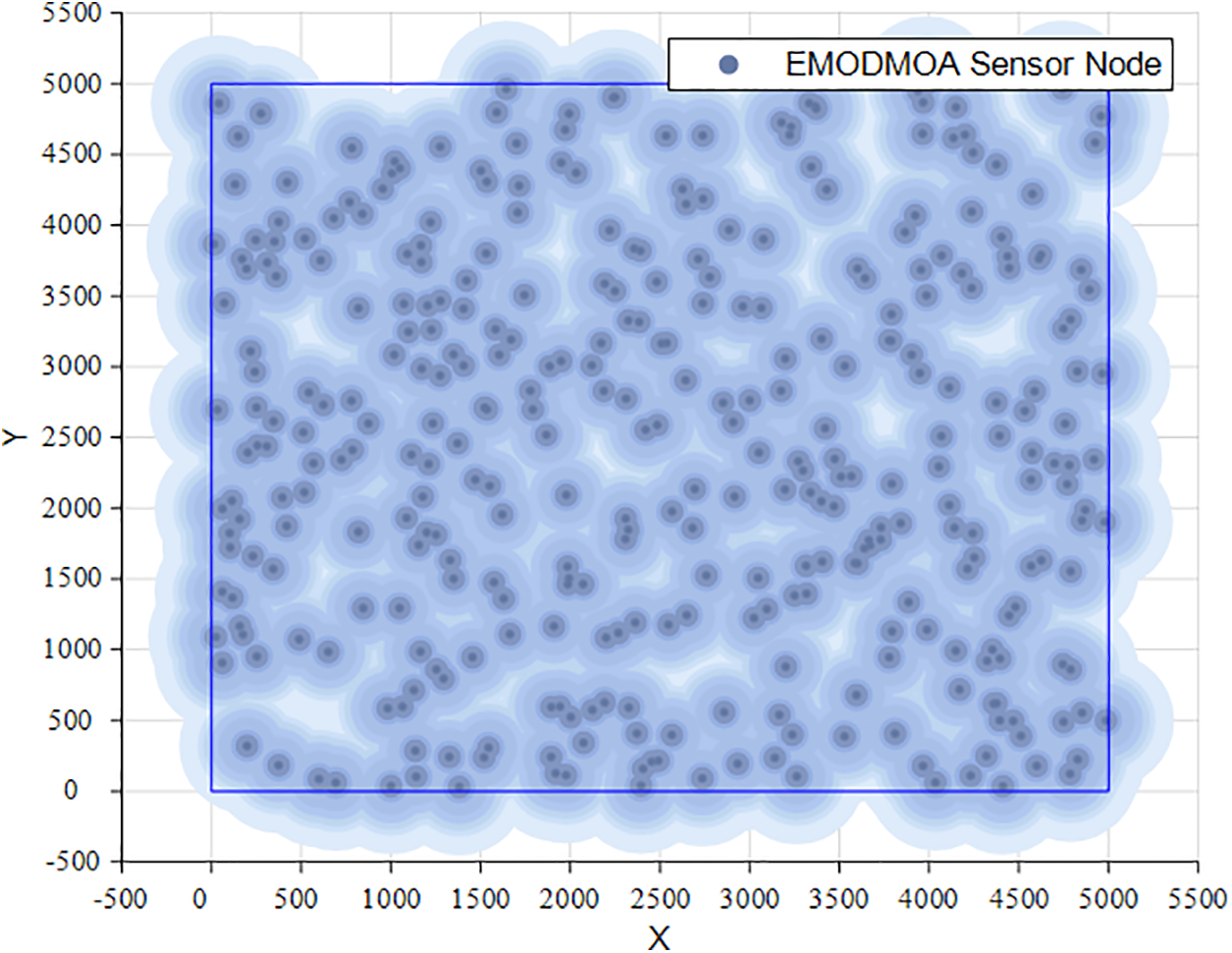
Figure 20: 5000 m × 5000 m range and 300 nodes

Case 4: 100 nodes are deployed within a 5000 m × 5000 m range, and the network coverage is as Fig. 21.

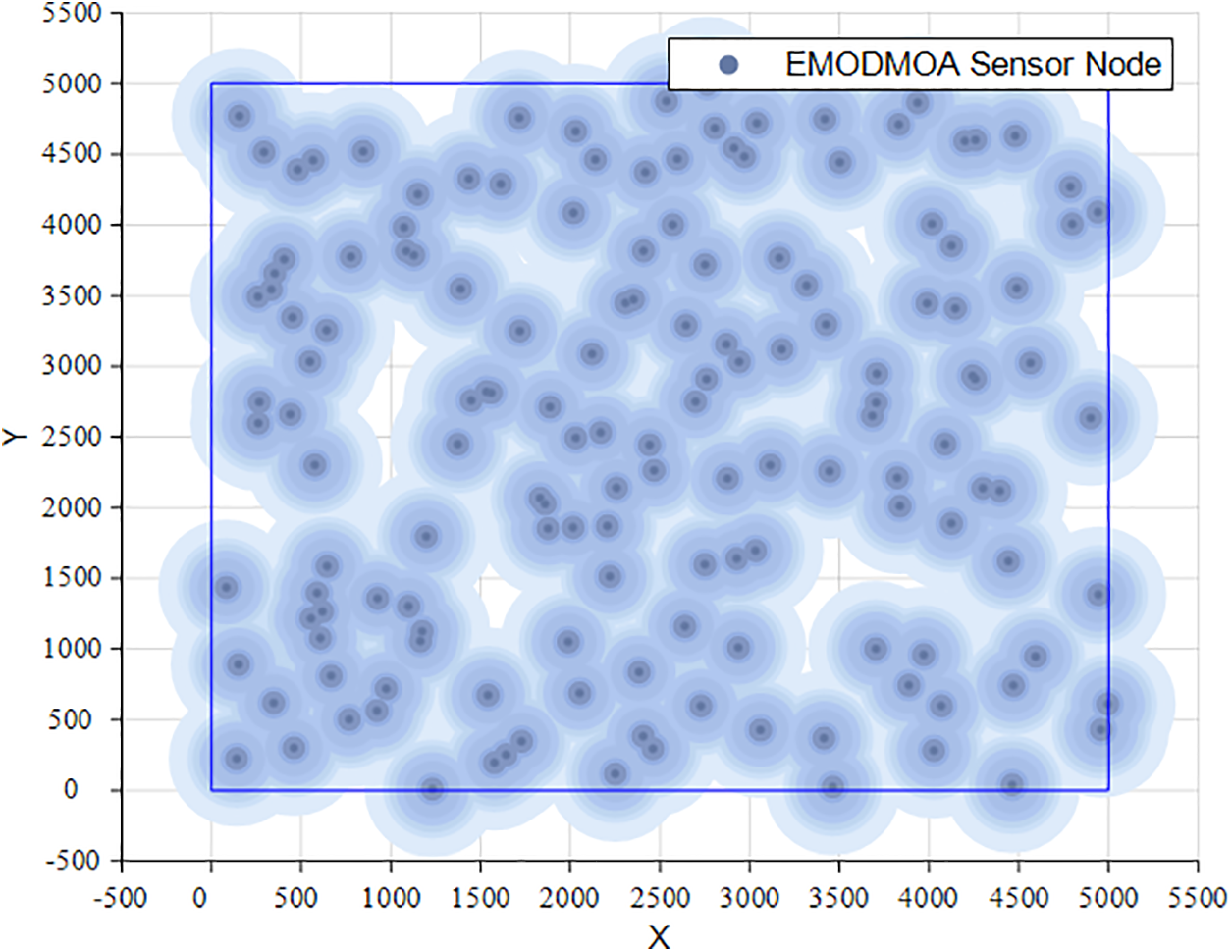
Figure 21: 5000 m × 5000 m range and 100 nodes

As can be seen from the coverage map of the wireless sensor network, the EMODMOA algorithm can optimize multi-node networks well and can ensure the uniform distribution of wireless sensor nodes, thus covering the target area well. For networks with a small number of wireless sensors, it is better than the limited number of sensors themselves, so full coverage of the target area cannot be guaranteed, but the sensors optimized by EMODMOA can also be distributed more evenly in the target area. As can be seen from the figure, both the large target area and the small target area can be well covered after optimization by the wireless sensor network.

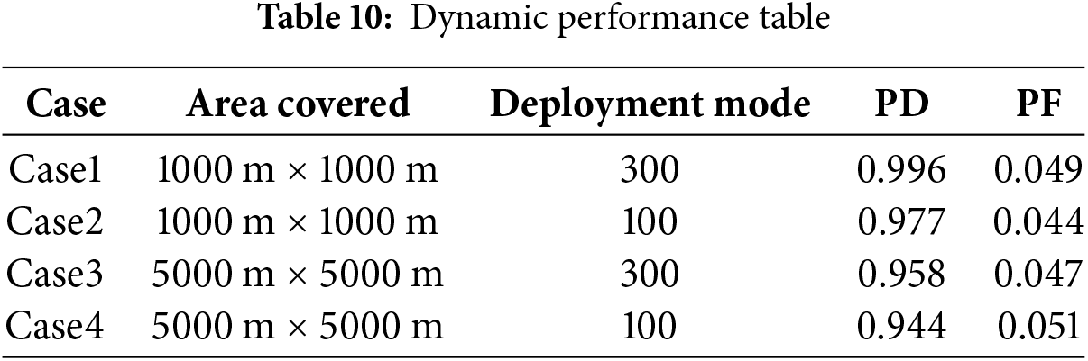
Table 10 shows the false alarm rate and detection rate after EMODMOA optimization in different cases. For the same target range, the more sensors there are, the lower the false alarm rate and the higher the detection rate. This shows that EMODMOA is suitable for optimizing multi-node networks. When the number of nodes is the same, the false alarm rate is low, and the detection rate is high for a small target area. In summary, EMODMOA is suitable for optimizing multi-wireless sensor node networks, and there is no limit on the range of the target area.

6.3 Large-Scale Deployment

To verify the performance of the algorithm in large-scale wireless sensor networks, we will add an experiment to deploy a large-scale wireless sensor network for verification.

The experimental parameters are set as shown in Table 11, with 400 wireless sensor network nodes deployed within a 5000 m × 5000 m area.

Figs. 22–26 show the optimization of the network life cycle, spatial coverage, temporal coverage, false alarm rate, and detection rate of large-scale networks. Fig. 22 shows that EMODMOA has extended the network cycle from 70 to 87. Fig. 23 shows that EMODMOA has improved spatial coverage by 17%. Fig. 24 shows that EMODMOA has improved spatial coverage by 3%. Figs. 25–26 show that after EMODMOA optimization, the network false alarm rate has been greatly reduced and the network detection rate has been greatly improved. The EMODMOA algorithm has greatly extended the network life cycle, improved the spatial coverage and temporal coverage, greatly reduced the false alarm rate, and improved the detection rate of the network. Fig. 27 shows that EMODMOA can be used for large-scale deployment.

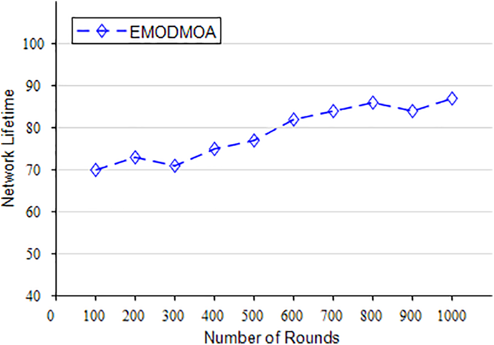
Figure 22: The network lifetime of large-scale deployment

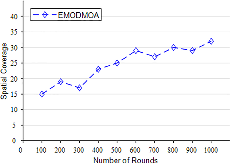
Figure 23: The spatial coverage of large-scale deployment

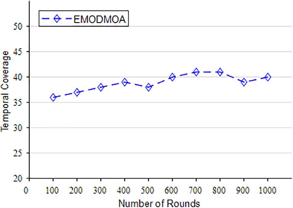
Figure 24: The temporal coverage of large-scale deployment

Figure 25: The PF of large-scale deployment

Figure 26: The PD of large-scale deployment

Figure 27: Large-scale deployment

7  Conclusion and Future Work

In this paper, an EMODMOA algorithm is proposed, which solves the problem of deploying a five-target SDFWSN. The algorithm improves the original DMOA algorithm by balancing the exploration and exploitation phases of the algorithm, thereby improving the convergence speed of the algorithm and preventing the algorithm from getting stuck in a local optimum. Using the KNN algorithm to select reference points can obtain various feasible solutions. The CEC2020 multi-objective multimodal optimization benchmark function was tested on the proposed algorithm, and the results showed that the algorithm was superior to other multi-objective algorithms used for comparison. Experiments on the deployment of SDFWSN were conducted in this paper. When the algorithm is applied to SDFWSN, it outperforms NSGAII, MOPSO, MOEA/D, and MOGWO in terms of HV, Delta, and NDS metrics. To verify the feasibility of the algorithm, cross-case deployment, and large-scale deployment are carried out. In the experiment, the algorithm can improve the spatial coverage and network survival rate, while improving the detection rate and reducing the false alarm rate. The algorithm proposed in this paper effectively solves the deployment problem of two-dimensional planar SDFWSN.

However, the algorithm proposed in this study cannot well optimize the deployment of a network with few sensors in a large target area, and the model applied in the experiment can also be further optimized to make it more in line with practical applications. Therefore, in future work, we will focus on optimizing the model of a network with few sensors in a large target area, solve practical problems that affect the deployment of wireless sensors, and consider more realistic factors in the construction of the model, to achieve a model that is more in line with practical applications. We will deploy this network and verify the randomness of wireless sensor perception based on data fusion.

Acknowledgment: The authors thank the National Natural Science Foundation of China and Innovation Project of Guangxi Graduate Education for supporting this work.

Funding Statement: This work was supported by the National Natural Science Foundation of China under Grant Nos. U21A20464, 62066005 and Innovation Project of Guangxi Graduate Education under Grant No. YCSW2024313.

Author Contributions: The authors confirm contribution to the paper as follows: draft manuscript preparation: Shumin Li; analysis and interpretation of results, supervision; Qifang Luo; algorithm design, writing—review: Yongquan Zhou. All authors reviewed the results and approved the final version of the manuscript.

Availability of Data and Materials: The original contributions presented in the study are included in the article, further inquiries can be directed to the corresponding authors.

Ethics Approval: Not applicable.

Conflicts of Interest: The authors declare no conflicts of interest to report regarding the present study.

References

1. Elhabyan R, Shi W, St-Hilaire M. Coverage protocols for wireless sensor networks: review and future directions. J Commun Netw. 2019;21(1):45–60. [Google Scholar]

2. Wang SC, Hsiao HC, Lin CC, Chin H. Multi-objective wireless sensor network deployment problem with cooperative distance-based sensing coverage. Mob Netw Appl. 2022;27(1):1–12. [Google Scholar]

3. Sharma J, Bhutani A. Review on deployment, coverage and connectivity in wireless sensor networks. In: 2022 IEEE World Conference on Applied Intelligence and Computing (AIC); 2022; Sonbhadra, India. p. 802–7. [Google Scholar]

4. Abdollahzadeh S, Navimipour NJ. Deployment strategies in the wireless sensor network: a comprehensive review. Comput Commun. 2016;91–92:1–16. [Google Scholar]

5. Tan R, Xing G. Spatiotemporal coverage in fusion-based sensor networks. In: Ammari H, editor. The art of wireless sensor networks. Berlin, Heidelberg: Signals and Communication Technology Springer; 2013. p. 117–65. [Google Scholar]

6. Mohamed SM, Hamza HS, Saroit IA. Coverage in mobile wireless sensor networks (M-WSNa survey. Comput Commun. 2017;110:133–50. [Google Scholar]

7. Chaudhary DK, Dua RL. Application of multi objective particle swarm optimization to maximize coverage and lifetime of wireless sensor network. Int J Comput Eng Res. 2012;2:1628–33. [Google Scholar]

8. More A, Raisinghani V. A survey on energy efficient coverage protocols in wireless sensor networks. J King Saud Univ-Comput Inf Sci. 2017;29(4):428–48. doi:10.1016/j.jksuci.2016.08.001. [Google Scholar] [CrossRef]

9. Khalil EA, Ozdemir S. Reliable and energy efficient topology control in probabilistic wireless sensor networks via multi-objective optimization. J Supercomput. 2017;73(6):2632–56. doi:10.1007/s11227-016-1946-x. [Google Scholar] [CrossRef]

10. Chelbi S, Dhahri H, Bouaziz R. Node placement optimization using particle swarm optimization and iterated local search algorithm in wireless sensor networks. Int J Commun Syst. 2021;34(9):e4813. doi:10.1002/dac.4813. [Google Scholar] [CrossRef]

11. Jaiswal K, Anand V. A QoS aware optimal node deployment in wireless sensor network using Grey wolf optimization approach for IoT applications. Telecommun Syst. 2021;78(4):559–76. doi:10.1007/s11235-021-00831-9. [Google Scholar] [CrossRef]

12. Moustafa G, El-Rifaie AM, Smaili IH, Ginidi A, Shaheen AM, Youssef AF, et al. An enhanced dwarf mongoose optimization algorithm for solving engineering problems. Mathematics. 2023;11(15):3297. doi:10.3390/math11153297. [Google Scholar] [CrossRef]

13. Agushaka JO, Ezugwu AE, Abualigah L. Dwarf mongoose optimization algorithm. Comput Methods Appl Mech Eng. 2022;391:11457. [Google Scholar]

14. Elaziz MA, Ewees AA, Al-Qaness MAA, Alshathri S, Ibrahim RA. Feature selection for high dimensional datasets based on quantum-based dwarf mongoose optimization. Mathematics. 2022;10(23):4565. [Google Scholar]

15. Tahmasebi S, Rasouli N, Kashefi AH, Rezabeyk E, Faragardi HR. SYNCOP: an evolutionary multi-objective placement of SDN controllers for optimizing cost and network performance in WSNs. Comput Netw. 2021;185:107727. [Google Scholar]

16. Hajjej F, Hamdi M, Ejbali R, Zaied M. A new optimal deployment model of internet of things based on wireless sensor networks. In: 2019 15th International Wireless Communications & Mobile Computing Conference (IWCMC); 2019; Tangier, Morocco. p. 2092–7. [Google Scholar]

17. Wang P, Xiong Y, She J. A new closed-barrier covering optimization method for heterogeneous nodes in hybrid wireless sensor networks. In: IECON 2021-47th Annual Conference of the IEEE Industrial Electronics Society; 2021; Toronto, ON, Canada. p. 1–6. [Google Scholar]

18. Metiaf A, Wu Q. Wireless sensor network deployment optimization using reference-point-based non-dominated sorting approach (NSGA-Ⅲ) Asia Pacific Institute of Science and Engineering. In: Proceedings of 2019 3rd International Conference on Data Mining, Communications and Information Technology (DMCIT 2019); 2019; Beijing, China: IOP Publishing. [Google Scholar]

19. Dahmane WM, Dollinger JF, Ouchani S. A BIM-based framework for an optimal WSN deployment in smart building. In: 2020 11th International Conference on Network of the Future (NoF). Bordeaux, France; 2020. p. 110–4. [Google Scholar]

20. Saad A, Senouci MR, Benyattou O. Toward a realistic approach for the deployment of 3D Wireless Sensor Networks. IEEE Trans Mob Comput. 2020;21(4):1508–19. [Google Scholar]

21. Zaimen K, Brahmia MEA, Dollinger JF, Moalic L, Abouaissa A, Idoumghar L. A overview on WSN deployment and a novel conceptual BIM-based approach in smart buildings. In: 2020 7th International Conference on Internet of Things: Systems, Management and Security (IOTSMS); 2020; Paris, France. p. 1–6. [Google Scholar]

22. Mazloomi N, Gholipour M, Zaretalab A. Efficient configuration for multi-objective QoS optimization in wireless sensor network. Ad Hoc Netw. 2022;125:102730. [Google Scholar]

23. Chen L, Xu Y, Xu F, Hu Q, Tang Z. Balancing the trade-off between cost and reliability for wireless sensor networks: a multi-objective optimized deployment method. Appl Intell. 2023;53(8):9148–73. doi:10.1007/s10489-022-03875-9. [Google Scholar] [CrossRef]

24. Tang Y, Huang D, Li R, Huang Z. A non-dominated sorting genetic algorithm based on voronoi diagram for deployment of wireless sensor networks on 3-D terrains. Electronics. 2022;11(19):3024–4. doi:10.3390/electronics11193024. [Google Scholar] [CrossRef]

25. Zhang L, Liu T, Ding X. Large-scale WSNs resource scheduling algorithm in smart transportation monitoring based on differential ion coevolution and multi-objective decomposition. IEEE Trans Intell Transp Syst. 2024 Jan;25(1):829–38. doi:10.1109/TITS.2022.3208699. [Google Scholar] [CrossRef]

26. Mikitiuk A, Trojanowski K. Maximization of the sensor network lifetime by activity schedule heuristic optimization. Ad Hoc Netw. 2020;96:101994. doi:10.1016/j.adhoc.2019.101994. [Google Scholar] [CrossRef]

27. Zhao X, Cui Y, Guo Z, Hao Z. An energy-efficient coverage enhancement strategy for wireless sensor networks based on a dynamic partition algorithm for cellular grids and an improved vampire bat optimizer. Sensors. 2020;20(3):619. doi:10.3390/s20030619. [Google Scholar] [PubMed] [CrossRef]

28. Sadoun AM, Najjar IR, Alsoruji GS, Wagih A, Abd Elaziz M. Utilizing a long short-term memory algorithm modified by dwarf mongoose optimization to predict thermal expansion of Cu-Al2O3 nanocomposites. Mathematics. 2022;10(7):1050. doi:10.3390/math10071050. [Google Scholar] [CrossRef]

29. Akinola Olatunji A, Ezugwu Absalom E, Oyelade Olaide N, Agushaka Jeffrey O. A hybrid binary dwarf mongoose optimization algorithm with simulated annealing for feature selection on high dimensional multi-class datasets. Sci Rep. 2022;12(1):14945. doi:10.1038/s41598-022-18993-0. [Google Scholar] [PubMed] [CrossRef]

30. Agushaka JO, Akinola O, Ezugwu AE, Oyelade ON, Saha AK. Advanced dwarf mongoose optimization for solving CEC, 2011 and CEC, 2017 benchmark problems. PLoS One. 2022;17(11):e0275346. doi:10.1371/journal.pone.0275346. [Google Scholar] [PubMed] [CrossRef]

31. Mehmood K, Chaudhary NI, Khan ZA, Cheema KM, Raja MA, Milyani AH, et al. Dwarf mongoose optimization metaheuristics for autoregressive exogenous model identification. Mathematics. 2022;10(20):3821. doi:10.3390/math10203821. [Google Scholar] [CrossRef]

32. Agushaka JO, Ezugwu AE, Olaide ON, Akinola O, Zitar RA, Abualigah L. Improved dwarf mongoose optimization for constrained engineering design problems. J Bionic Eng. 2023;20(3):1263–95. doi:10.1007/s42235-022-00316-8. [Google Scholar] [PubMed] [CrossRef]

33. Akinola OA, Agushaka JO, Ezugwu AE. Binary dwarf mongoose optimizer for solving high-dimensional feature selection problems. PLoS One. 2022;17(10):e0274850. doi:10.1371/journal.pone.0274850. [Google Scholar] [PubMed] [CrossRef]

34. Alissa KA, Elkamchouchi H, Tarmissi D, Yafoz K, Alsini A, Alghushairy R, et al. Dwarf mongoose optimization with machine-learning-driven ransomware detection in internet of things environment. Appl Sci. 2022;12(19):9513. doi:10.3390/app12199513. [Google Scholar] [CrossRef]

35. Alrayes FS, Alzahrani JS, Alissa KA, Alharbi A, Alshahrani H, Elfaki MA, et al. Dwarf mongoose optimization-based secure clustering with routing technique in internet of drones. Drones. 2022;6(9):247. doi:10.3390/drones6090247. [Google Scholar] [CrossRef]

36. Balasubramaniam S, Satheesh Kumar K, Kavitha V, Prasanth A, Sivakumar TA. Feature selection and dwarf mongoose optimization enabled deep learning for heart disease detection. Comput Intell Neurosci. 2022;2022:2819378. doi:10.1155/2022/2819378. [Google Scholar] [PubMed] [CrossRef]

37. Zare P, Davoudkhani IF, Zare R, Ghadimi H, Sabery B, Abad AB. Optimum operation of grid-independent microgrid considering load effect on lifetime characteristic of battery energy storage system using dwarf mongoose optimization algorithm. In: 2023 8th International Conference on Technology and Energy Management (ICTEM); 2023; Babol, Iran. p. 1–7. [Google Scholar]

38. Dora BK, Bhat S, Halder S, Sahoo M. Solution of reactive power dispatch problems using enhanced dwarf mongoose optimization algorithm. In: 2023 International Conference for Advancement in Technology (ICONAT); 2023; Goa, India. p. 1–6. [Google Scholar]

39. Fu S, Huang H, Ma C, Wei J, Li Y, Fu Y. Improved dwarf mongoose optimization algorithm using novel nonlinear control and exploration strategies. Expert Syst Appl. 2023;233:120904. doi:10.1016/j.eswa.2023.120904. [Google Scholar] [CrossRef]

40. Abirami A, Kavitha R. An efficient early detection of diabetic retinopathy using dwarf mongoose optimization based deep belief network. Concurr Comput-Pract Exp. 2022;34(28). doi:10.1002/cpe.v34.28. [Google Scholar] [CrossRef]

41. Almutairi L, Daniel R, Khasimbee S, Lydia EL, Acharya S, Kim HI. Quantum dwarf mongoose optimization with ensemble deep learning based intrusion detection in cyber-physical systems. IEEE Access. 2023;11:66828–37. doi:10.1109/ACCESS.2023.3287896. [Google Scholar] [CrossRef]

42. Rizk-Allah RM, El-Fergany AA, Gouda EA, Kotb MF. Characterization of electrical 1-phase transformer parameters with guaranteed hotspot temperature and aging using an improved dwarf mongoose optimizer. Neural Comput Appl. 2023;35(19):13983–98. doi:10.1007/s00521-023-08449-5. [Google Scholar] [CrossRef]

43. Li D, Hu YH. Energy-based collaborative source localization using acoustic microsensor array. EURASIP J Adv Signal Process. 2003;2003(4):1–17. doi:10.1155/S1110865703212075. [Google Scholar] [CrossRef]

44. Randhawa S, Jain S. An intelligent PSO-based energy efficient load balancing multipath technique in wireless sensor networks. Turkish J Electr Eng Comput Sci. 2017;25(4):3113–31. doi:10.3906/elk-1606-206. [Google Scholar] [CrossRef]

45. Wang J, Yang X, Ma T, Wu M, Kim JU. An energy-efficient competitive clustering algorithm for wireless sensor networks using mobile sink. Int J Grid Distrib Comput. 2012;5(4):79–92. [Google Scholar]

46. Zhang Y, Yu W, Chen X, Jiang J. Parallel genetic algorithm to extend the lifespan of internet of things in 5G networks. IEEE Access. 2020;8:149630–42. [Google Scholar]

47. Zitzler E, Thiele L, Laumanns M, Fonseca CM, Da Fonseca VG. Performance assessment of multiobjective optimizers: an analysis and review. IEEE Trans Evol Comput. 2003;7(2):117–32. [Google Scholar]

48. Zhou A, Zhang Q, Jin Y. Approximating the set of Pareto-optimal solutions in both the decision and objective spaces by an estimation of distribution algorithm. IEEE Trans Evol Comput. 2009;13(5):1167–89. [Google Scholar]

49. Yue C, Qu B, Liang J. A multiobjective particle swarm optimizer using ring topology for solving multimodal multiobjective problems. IEEE Trans Evol Comput. 2017;22(5):805–17. [Google Scholar]

50. Guo J, Jafarkhani H. Sensor deployment with limited communication range in homogeneous and heterogeneous wireless sensor networks. IEEE Trans Wirel Commun. 2016;15(10):6771–84. doi:10.1109/TWC.2016.2590541. [Google Scholar] [CrossRef]