An Improved Local RBF Collocation Method for 3D Excavation Deformation Based on Direct Method and Mapping Technique

1  Introduction

The excavation is a kind of retaining structure, which is usually performed in congested urban areas to ensure the safety of the underground space [1,2]. The deformation is a key indicator used to assess the stability of excavation. Investigators have carried out a lot of numerical methods to calculate and predict excavation deformation [3,4], but some difficulties still exist in the numerical simulation of excavation. One of the difficulties comes from the elastic-plasticity of soil. The Drucker-Prager (D-P) model [5,6], which is modified from the Mises yield model and takes into account the influence of the first stress invariant, is usually used to describe the plasticity in the soil. In order to deal with the elastic-plastic deformation, the incremental theory is applied to reflect the influence of the stress path. However, the incremental theory is based on the accurate and stable calculation in each incremental step, otherwise the error would continuously accumulate. Additionally, the size effect caused by various excavation shapes is often present in excavation engineering, such as the circular excavation [7,8]. The circular excavation shape can reduce the lateral deformation due to the circumferential hoop force. Therefore, a three-dimensional (3D) geotechnical model with a relatively complex shape is necessary for excavation simulation. A typical excavation is mainly composed of the soil and support structure which must be considered separately. In this structure, the support part typically has a large length-width ratio. It is not efficient to use the same node arrays or elements in different axis directions for this kind of 3D problem.

The finite element method (FEM) is commonly used to simulate the practical problems of excavation [7,9,10]. Although the FEM has the advantages such as a simple principle and strong adaptability, some meshless methods show advantages over the FEM in computational efficiency, accuracy, solving high-dimensional problems, and handling complex geometries [11]. In the last decade, some meshless methods were applied to solve boundary value problems, such as the method of the fundamental solution [12] and the boundary knot method [13]. In order to avoid dense matrices, various localized techniques have been employed, leading to the development of many different localized methods, such as the localized boundary knot method [14] and the localized method of fundamental solutions [15]. The local radial basis function collocation method (LRBFCM), which is modified from the global radial basis function collocation method, and the interpolation calculation is applied in a local domain, is one of the famous localized meshless methods [16–18]. By using LRBFCM, some elastic-plasticity problems and other nonlinear problems could be solved [19–21]. Our tests have shown that the traditional LRBFCM is difficult to directly combine with the incremental method for solving elastic-plastic excavation problems, as its accuracy and stability need improvement. The traditional LRBFCM exhibits poor accuracy in solving first-order derivatives, as analyzed in reference [11]. These first-order derivatives are prevalent in the excavation problems, as they arise not only from the stress boundary conditions but also from the governing equations themselves. Additionally, the accuracy of the RBF collocation method is greatly influenced by the value of the shape parameter. Although there is no universal and simple method to obtain the optimal shape parameters so far, scholars have realized that the shape parameters are mainly influenced by the Euclidean distances between collocation nodes [22–24]. Zheng et al. [11] proposed the direct method, where the nodes on a straight line are used to construct the first-order derivative matrix to address the instability problem in dealing with Neumann boundary conditions. This method can also significantly improve the accuracy of the computation of first-order partial derivatives. Through further research, the direct method can be extended to the partial derivative computation for interior nodes to improve the computational accuracy and reduce the influence of shape parameters [25]. Furthermore, we find the direct method could also improve calculation efficiency in the simulation of the large length-width ratio shape problems, such as the excavation’s support structure in this work.

In actual excavation engineering, excavations often have irregular shapes, which are difficult to describe in simulations. There are many numerical methods available for solving problems with complex boundary shapes, including the localized boundary knot method [14], the radial basis function collocation method (RBFCM) [26], and the method of approximate particular solutions (MAPS) [27]. Zheng et al. [11] applied the fictitious nodes method to optimized the LRBFCM to solve the arbitrary shape problems, but the efficiency of describing irregular boundary shapes with this method is still not high enough for the excavation problems. Wen et al. [28,29] proposed the mapping technique in the finite block method (FBM) for the shape problems. By using the mapping technique, a quadratic-type domain was transformed from physical coordinates to normalized coordinates. The partial differential operators in the irregular physical domain were addressed by differential operators in the transformed normalized domain. The collocation nodes in this normalized domain can be distributed uniformly [30,31]. In this paper, the mapping technique is applied to LRBFCM to solve excavation problems. The irregular shape of the 3D excavation is described using several quadratic-type blocks.

In this paper, the optimized LRBFCM is applied in 3D excavation deformation calculation. The direct method and the mapping technique is employed to improve the traditional LRBFCM, making it possible to apply the LRBFCM to excavation problems and harnessing the algorithm’s advantages in accuracy and efficiency.

2  LRBFCM and the Numerical Technique

2.1 Indroduction of the LRBFCM

In the formulation of LRBFCM, the field variable u can be approximated by

u(x)=∑k=1nsϕ(‖x−xk‖)αk,(1)

where ns is the number of local nodes, αk is the undetermined coefficient, ϕ is radial basis function (RBF). In this work, the following multi-quadratic (MQ) RBF is employed:

ϕ(rk)=rk2+c2,

where c is the shape parameter and rk=‖x−xk‖ denotes the Euclidean distance between points x and xk. For traditional LRBFCM, the nearest neighboring nodes of the observation node are usually employed as the local nodes {xk},1≤k≤ns. Fig. 1 shows the condition of the local nodes as ns=5.

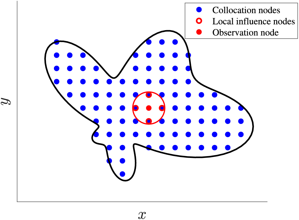
Figure 1: Sketch of the local nodes as ns=5

In the local influence domain, x∈{xj},1≤j≤ns, and the solution is approximated by

u¯=ϕ¯α,(2)

where

u¯=[u(x1),u(x2),⋯,u(xns)]T,ϕ¯=[ϕ(‖xj−xk‖)]1≤j,k≤ns,α=[α1,α2,⋯,αns]T.

The Eq. (2) can be rewritten as

α=ϕ¯−1u¯.(3)

Substituting Eq. (3) into Eq. (1), the field quantity and its differential form can be expressed as

u(x)=ϕ′ϕ¯−1u¯,(4)

ℒu(x)=ℒϕ′ϕ¯−1u¯,(5)

where ℒ is the differential operator, ϕ′=[ϕ(‖x−x1‖),ϕ(‖x−x2‖),⋯,ϕ(‖x−xns‖)] and ℒϕ′=[ℒϕ(‖x−x1‖),ℒϕ(‖x−x2‖),⋯,ℒϕ(‖x−xns‖)] are vectors with the size of 1×ns. Let Φ¯=ϕ′ϕ¯−1 and ℒΦ¯=ℒϕ′ϕ¯−1. By strategically adding zero elements in appropriate positions, Φ¯ and ℒΦ¯ can be converted into the global sparse vectors Φ~ and ℒΦ~ with the size of 1×n, where n is the total number of global collocation nodes:

local Φ¯⇒global Φ~,(6)

local ℒΦ¯⇒global ℒΦ~,(7)

local u¯⇒global u~,(8)

where u~=[u(x1),u(x2),⋯,u(xn)] is the vector of field variable in the global domain. Then Eqs. (4) and (5) can be expressed as

u(x)=Φ¯u¯=Φ~u~,(9)

ℒu(x)=ℒΦ¯u¯=ℒΦ~u~.(10)

The unknown field variable vector u~ can be derived from governing partial differential equations and boundary conditions by considering Eqs. (9) and (10).

2.2 The Direct Method and Optimization of the Local Nodes

The direct method is adopted to optimize the local nodes. Instead of using the nearest neighboring nodes, the direct method selects only the nearest nodes in the n direction as the local influence nodes to calculate the first order partial derivative ∂u∂n. Fig. 2 shows a condition of local points in 2D. As shown in the figure, we use three points along the x-axis to express ∂u∂x and another three points along the y-axis to calculate ∂u∂y. This method can be fully extended to 3D conditions.

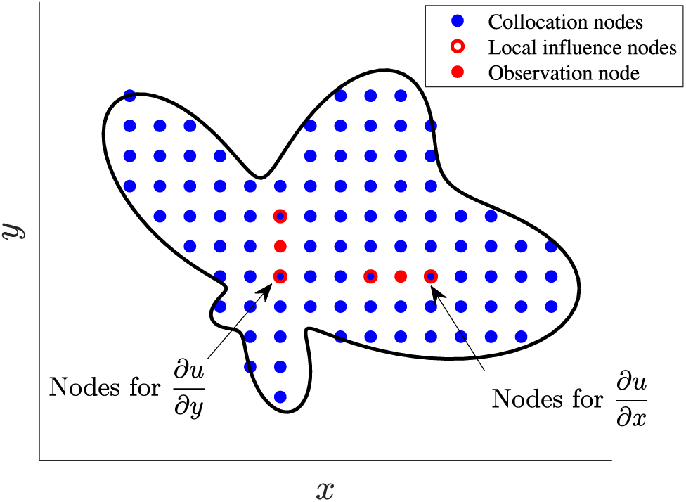
Figure 2: A condition of local points for the direct method

The local influence points of direct method is on a one-dimensional line, rather than in a circular configuration for two-dimension (or a spherical configuration for three-dimension). By introducing this method, the accuracy, efficiency, and stability of excavation problems would improve obviously: Firstly, a 2D or 3D problem is transformed into a 1D problem, as the local nodes are collocated along a straight line. This reduces the complexity of the calculation and improves the accuracy of the partial derivatives. Secondly, the direct method employs much fewer local points, leading to improved calculation efficiency. The direct method uses different nodes to address the partial derivatives in each coordinate direction, allowing for different point spacings to be considered in different directions. This feature is crucial for large length-width ratio shape problems, such as the support structure of excavation. Fig. 3 shows two different kinds of collocation node arrangements for a 2×0.1 bar in 2D. For the traditional LRBFCM, nodes should be uniformly distributed, as shown in Fig. 3a, to yield acceptable results. However, this arrangement results in too little node spacing in the x-axis direction limited by the size in the y-axis direction. The sparser nodes in x-axis, contrasting with y-axis, as shown in Fig. 3b, can be employed for the direct method and yield almost the same result. The much fewer collocation nodes in the direct method lead to a significant improvement in computational efficiency. Lastly, the influence of the shape parameters is greatly reduced by using the direct method to optimize the traditional LRBFCM. Thus, the simulation results will have greater stability. As we know, the optimal shape parameter of RBFs collocation method is primarily determined by the Euclidean distances between the local nodes [22]. For the direct method, the positional relationship of the three local points is stationary. The shape parameter c would have a sufficiently wide acceptable value range, which would be further proposed in the examples in Section 5. In fact, we would use the value c/d instead of c in the cases where d is the Euclidean distance between the nearest local nodes to adapt the shape parameter for different d and further ensure the rationality of the shape parameter.

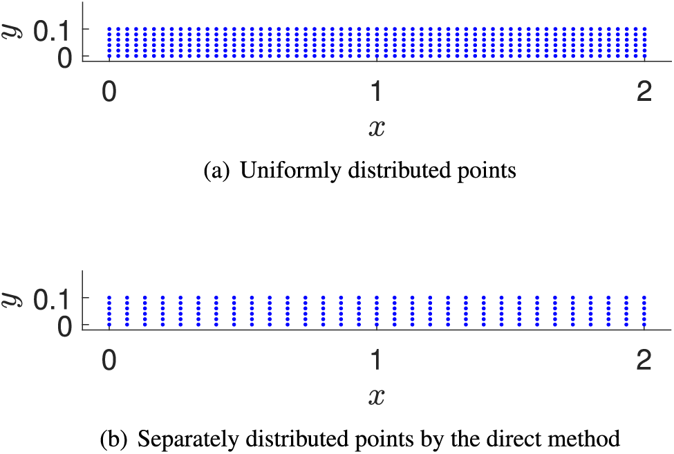
Figure 3: Collocation points for different methods

However, the direct method still requires the nodes to be neatly arranged in the direction of partial derivative n. This means that the direct method can only be applied to a rectangular domain in 2D (or a cuboid domain in 3D) directly. For the irregular-shaped domains, an additional technique needs to be employed.

3  Coordinate Transform and Mapping Technique in 3D

To solve the irregular shape domain problems, we use the mapping technique to transform physical coordinates (x,y,z) of a block of quadratic-type into normalized coordinates (κ,η,ν), where −1≤κ,η,ν≤1. For the 3D problem, a normalised block with 20 seeds {(κi,ηi,νi)},1≤i≤20 is shown in Fig. 4. The shape functions are given by

Ni=18(1+κiκ)(1+ηiη)(1+νiν)(κiκ+ηiη+νiν−2),i=1,2,3,4,5,6,7,8,(11)

Ni=14(1−κ2)(1+ηiη)(1+νiν),i=9,11,17,19,(12)

Ni=14(1−η2)(1+κiκ)(1+νiν),i=10,12,18,20,(13)

Ni=14(1−ν2)(1+κiκ)(1+ηiη),i=13,14,15,16.(14)

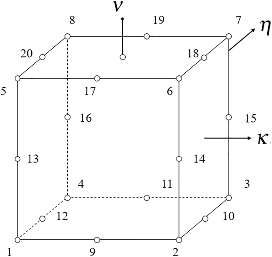
Figure 4: Normalised block and its mapping seeds

The partial differentials of shape functions are:

∂Ni∂κ=κi8(1+ηiη)(1+νiν)(2κiκ+ηiη+νiν−1),(15)

∂Ni∂η=ηi8(1+κiκ)(1+νiν)(κiκ+2ηiη+νiν−1),(16)

∂Ni∂ν=νi8(1+κiκ)(1+ηiη)(κiκ+ηiη+2νiν−1),i=1,2,3,4,5,6,7,8,(17)

∂Ni∂κ=−12κ(1+ηiη)(1+νiν),(18)

∂Ni∂η=14ηi(1−κ2)(1+νiν),(19)

∂Ni∂ν=14νi(1−κ2)(1+ηiη),i=9,11,17,19,(20)

∂Ni∂κ=14κi(1−η2)(1+νiν),(21)

∂Ni∂η=−12η(1+κiκ)(1+νiν),(22)

∂Ni∂ν=14νi(1−η2)(1+κiκ),i=10,12,18,20,(23)

∂Ni∂κ=14κi(1−ν2)(1+ηiη),(24)

∂Ni∂η=14ηi(1−ν2)(1+κiκ),(25)

∂Ni∂ν=−12ν(1+κiκ)(1+ηiη),i=13,14,15,16.(26)

Then the physical coordinate can be written as

x=∑i=120Ni(κ,η,ν)xi,y=∑i=120Ni(κ,η,ν)yi,z=∑i=120Ni(κ,η,ν)zi,(27)

where (xi,yi,zi) are the physical coordinates corresponding to the mapping seeds (κi,ηi,νi). Then the partial derivatives of field quantity are:

∂u∂x=1J(∂u∂κβ11+∂u∂ηβ12+∂u∂νβ13),∂u∂y=1J(∂u∂κβ21+∂u∂ηβ22+∂u∂νβ23),∂u∂z=1J(∂u∂κβ31+∂u∂ηβ32+∂u∂νβ33),(28)

J=|∂x∂κ∂x∂η∂x∂ν∂y∂κ∂y∂η∂y∂ν∂z∂κ∂z∂η∂z∂ν|,

β11=∂y∂η∂z∂ν−∂y∂ν∂z∂η,β12=−∂y∂κ∂z∂ν+∂y∂ν∂z∂κ,β13=∂y∂κ∂z∂η−∂y∂η∂z∂κ,β21=−∂x∂η∂z∂ν+∂x∂ν∂z∂η,β22=∂x∂κ∂z∂ν−∂x∂ν∂z∂κ,β23=−∂x∂κ∂z∂η+∂x∂η∂z∂κ,β31=∂x∂η∂y∂ν−∂x∂ν∂y∂η,β32=−∂x∂κ∂y∂ν+∂x∂ν∂y∂κ,β33=∂x∂κ∂y∂η−∂x∂η∂y∂κ.

By utilizing the mapping technique, the partial derivatives in the physical coordinate system of a quadratic-type block can be expressed in terms of partial differentials in the normalized coordinate system. In this normalized domain, the direct method, as described in Section 2.2, can be applied. For irregular shapes, such as circular excavation, the calculational domain should be subdivided into several quadratic-type blocks, and the interpolation is implemented in each block individually. Further details on the mapping technique can be found in references [28–31].

4  Governing Equations

In the excavation, the support structure is modeled as an elastic material, while the soil is simplified as an elastic-plastic body. This section provides a brief overview of elastic and elastic-plastic theories.

4.1 Elastic Theory

The equilibrium equations can be written as

∂σx∂x+∂τyx∂y+∂τzx∂z+fx=0,∂τxy∂x+∂σy∂y+∂τzy∂z+fy=0,∂τxz∂x+∂τyz∂y+∂σz∂z+fz=0,(29)

where σx, σy, σz are the normal stress components, and τyx=τxy,τzy=τyz,τxz=τzx are the shear stress components in the directions marked by the respective sub-indices, fx, fy, fz are the body force. For linear elasticity, the stress-strain relationship can be described as

σx=E(1−2ν)(1+ν)((1−ν)εx+νεy+νεz),τyx=τxy=E2(1+ν)γxy,σy=E(1−2ν)(1+ν)(νεx+(1−ν)εy+νεz),τzy=τyz=E2(1+ν)γyz,σz=E(1−2ν)(1+ν)(νεx+νεy+(1−ν)εz),τxz=τzx=E2(1+ν)γzx,(30)

where ν is the Poisson’s ratio, E denotes the Young’s modulus, {εx,εy,εz} are the normal strain, and {γxy, γyz, γzx} are shear strain components. The relations between strains and displacements are determined as follows:

εx=∂ux∂x,γxy=∂uy∂x+∂ux∂y,εy=∂uy∂y,γyz=∂uz∂y+∂uy∂z,εz=∂uz∂z,γzx=∂uz∂x+∂ux∂z,(31)

where {ux,uy,uz} are the displacement components. Aside from the partial differential governing equations, the displacement boundary can be described as

ux=u^x,uy=u^y,uz=u^z,(32)

where {ux^,uy^,uz^} represent the known displacement components. Then the stress boundary conditions can be written as

Tx=nxσx+nyτyx+nzτzx,Ty=nxτxy+nyσy+nzτzy,Tz=nxτxz+nyτyz+nzσz,(33)

where {Tx,Ty,Tz} represent the known force components. {nx,ny,nz} represent the cosine values of the angle between n and the axis {x,y,z}, where n is the boundary’s normal vector. For the elastic theory, the displacement components {ux,uy,uz} can be gained by solving the system of governing and boundary equations.

4.2 Elastic-Plastic Theory

For the classical elastic-plastic theory, the constitutive equations of an elastic-plastic body should be described in the incremental form [32,33]. Let dσ=[dσxdσydσzdτxydτyzdτzx]T and dε=[dεxdεydεzdγxydγyzdγzx]T represent the stress components and strain components in the respective directions marked by the sub-indices. Based on elastic-plastic theory, the strain increment can be divided into the elastic strain increment dεe and the plastic strain increment dεp:

dε=dεe+dεp.(34)

Then the stress-strain relation can be expressed as

dσ=Cedεe=Ce(dε−dεp),(35)

or

dσ=Cepdε,(36)

where Ce is elastic stiffness matrix and Cep is elastic-plastic stiffness matrix.

The plasticity of soil is described by the Drucker-Prager (D-P) model [5,6]. Its yield condition is defined as

g=αI1+J2−k(∫dεp¯)=0,(37)

where J2 stands for the second deviatoric stress invariant, and I1 stands for the first stress invariant. α and k denote the material parameters. In the initial yield condition, the parameters can be obtained by the friction angle φ and soil’s cohesion C as [2,32]

α=2sin⁡φ3(3−sin⁡φ),k=6Ccos⁡φ3(3−sin⁡φ).(38)

∫dεp¯ is the equivalent plastic strain. The flow law can be expressed as

dεp=Λ∂g∂σ,(39)

where Λ is a positive scalar called plastic multiplier, ∂g∂σ denotes the normal to the plastic potential. Let

Λ=1h[∂g∂σ]Tdσ,(40)

Cep=Ce−1HCe∂g∂σ[∂g∂σ]TCe,(41)

H=h+[∂g∂σ]TCe∂g∂σ.(42)

Due to the nonlinearity of elastic-plastic material, the stiffness matrix changes as the increase of equivalent plastic strain ∫dεp¯. The incremental theory is recommended to capture the evolution of stress along the loading path. Let f denote the total load applied during the loading process, and the stress path is artificially divided into s incremental steps. In each step, a load increment Δf=f/s is applied, and the stiffness matrix is updated based on the state at each collocation points. Consequently, the increments of displacement, strain, and stress are computed. Finally, all the increments are aggregated to field the total results.

5  Numerical Results and Discussion

In this section, we will present some numerical examples to show the effectiveness of the proposed numerical method. In these examples, the parameters are denoted in Table 1. In order to distinguish the LRBFCM optimized by the direct method from the traditional LRBFCM, we refer to the optimized version as D-LRBFCM. Considering that displacement is the key indicator to judge the safety of excavation, we mainly analyze the displacement fields of excavation. As we know, strain and stress can be obtained by the displacement fields. Since no analytical solution is available in these examples, we compare our numerical outcomes of the LRBFCM with FEM and the relative error (Rel) of maximum displacement is introduced to measure the errors:

Rel=||u~max|−|umax||umax||×100%,

where |u~max| and |umax| denote maximum displacements of the LRBFCM and FEM, respectively.

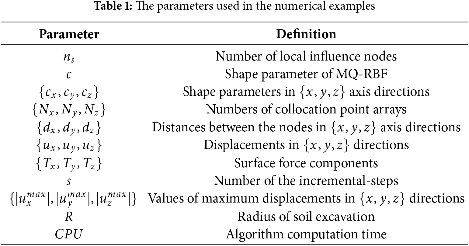
The mechanical parameters in these examples were determined with reference to literature [1–3] and in consideration of the local geotechnical conditions. In these numerical examples, the parameters of the support structure are Poisson’s ratio ν=0.2, Young’s modulus E=12,000MPa, and density ρ=2500kg/m3. The soil is assumed as homogeneous material for simplicity and the parameters are considered as Poisson’s ratio ν=0.35, elastic modulus E=8MPa, friction angle φ=17∘, cohesion C=6kPa, and unit weight γ=18kN/m3. The uniaxial compression test results of soil are shown in Fig. 5.

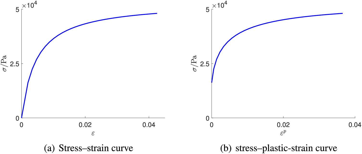
Figure 5: Uniaxial compression test results of soil

The numerical computations in this section were carried out using MATLAB© on a system equipped with an AMD EPYC Milan 7713 CPU (2.0 GHz), 64 GB of memory, and 16 cores, running CentOS Linux release 7.

5.1 Example 1

An elastic case is used to show the improvement of the D-LRBFCM. As shown in Fig. 6, there is a b×l×h pile, whose mechanical parameters are proposed as the support structure. The pile is fixed on z=0 side, bearing the gravity G and the load q=−104Pa on x=b side. The boundary conditions can be presented as follows:

Tx=0Pa,Ty=0Pa,Tz=0Pax=0m,Tx=q,Ty=0Pa,Tz=0Pax=b,Tx=0Pa,Ty=0Pa,Tz=0Pay=0m,Tx=0Pa,Ty=0Pa,Tz=0Pay=l,ux=0m,uy=0m,uz=0mz=0m,Tx=0Pa,Ty=0Pa,Tz=0Paz=h.

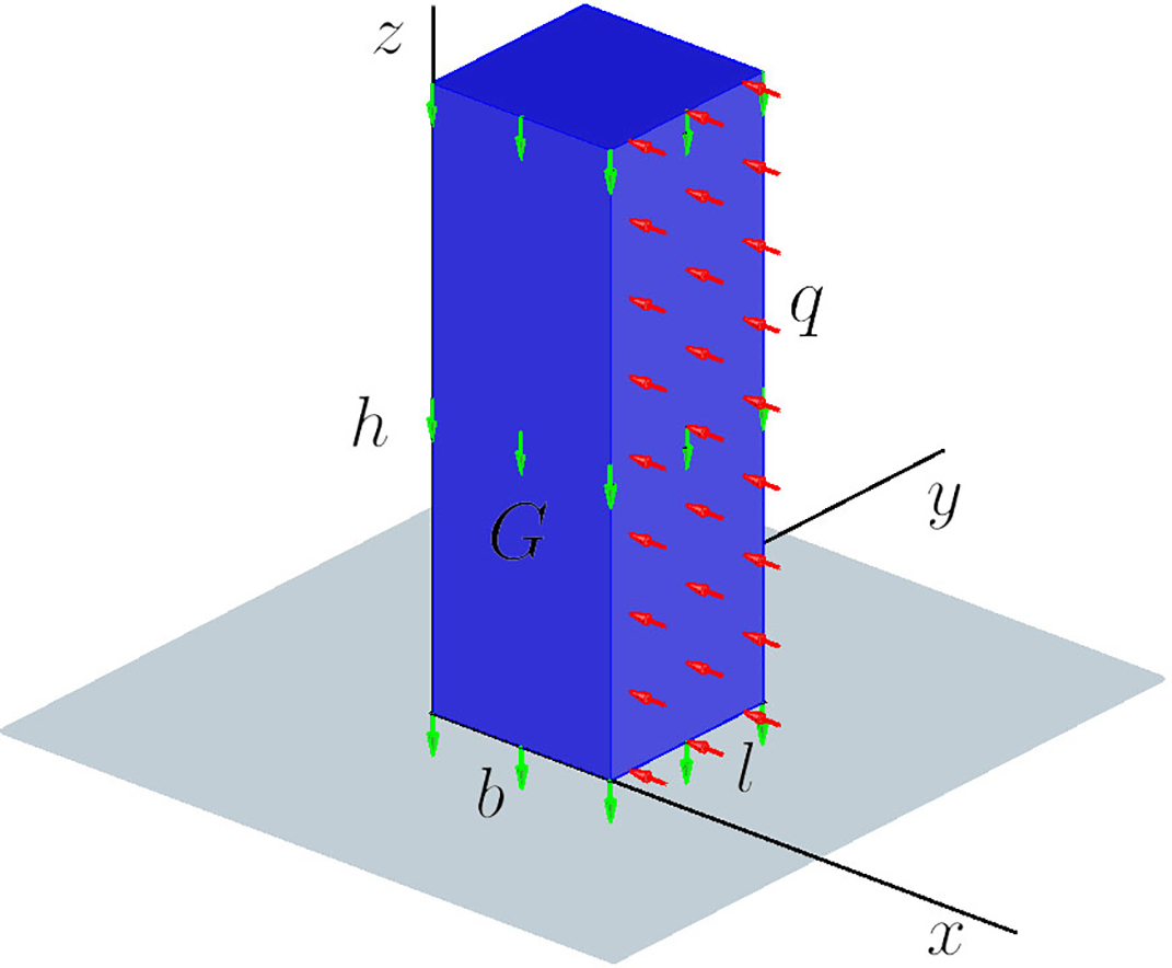
Figure 6: The mechanical state of Example 1

Firstly, we assume that b=l=1m, h=3m and the displacement results of FEM are shown in Fig. 7, where |uxmax| = 1.117e-4 m, |uymax| = 1.992e-6 m, and |uzmax| = 3.164e-5 m. {Nx,Ny,Nz}={21,21,61}, dx=dy=dz=0.05. ns=3 is used in the D-LRBFCM and ns=19 is used in the traditional LRBFCM, the numerical errors of the two methods under varying shape parameters are shown in Fig. 8. The results from the traditional LRBFCM are acceptable only when c=5, and they are sensitive to the shape parameter. In contrast, the numerical errors in the D-LRBFCM remain stable as the shape parameter varies from 0.5 to 700. Obviously, the stability of the D-LRBFCM is much better than that of the traditional LRBFCM. Combining with the analysis in the literature [22], we can infer a suitable range of shape parameters for the D-LRBFCM in 3D problems: 10<cx/dx,cy/dy,cz/dz<14,000. Since the accuracy of the D-LRBFCM is insensitive to the shape parameter, the parameter of D-LRBFCM cx/dx=cy/dy=cz/dz=100 is fixed for convenience through the rest of this section without further explanation.

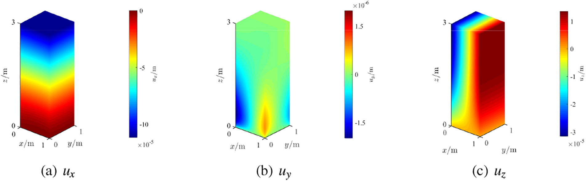
Figure 7: Displacement results of Example 1

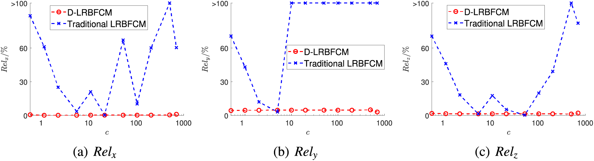
Figure 8: Numerical errors for different shape parameters c

Next, we consider the case where b=l=1m and h=3m. ns=3 is used in the D-LRBFCM, while c=5 and ns=19 are cosidered for the LRBFCM. Fig. 9 shows the accuracy under different node distributions, where CPU time represents the time used by the D-LRBFCM. We notice that the traditional LRBFCM only get relatively accurate results when the collocation points are evenly distributed in all the coordinate axis directions, which corresponds to the case where {Nx,Ny,Nz}={21,21,61}. Once the distribution of nodes becomes non-uniform, the calculation accuracy will decrease. By contrast, the change in node distributions has little effect on the calculation accuracy in D-LRBFCM, as the partial derivatives are calculated independently in different directions. Hence, by using the D-LRBFCM, we can employ a flexible and adaptable node array based on the deformation field of structure and the shape of the computational domain. In solving large length-width ratio problems, we can select fewer collocation nodes along the longer side, which leads to an improvement in computational efficiency. This can be reflected in the CPU time in Fig. 9.

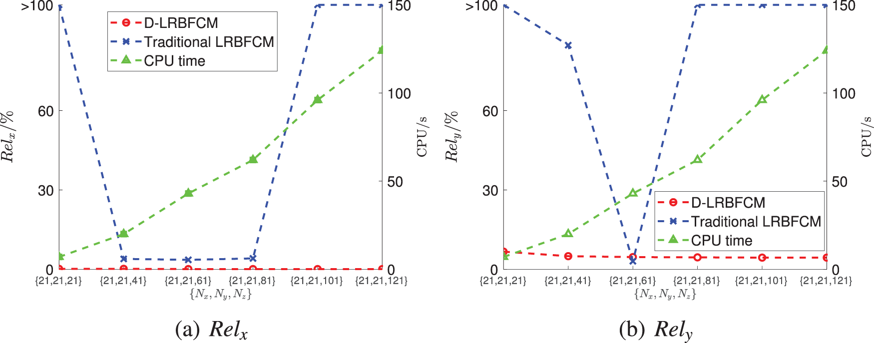
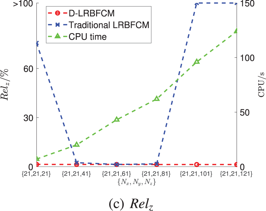
Figure 9: The accuracy under different node distributions

In order to assess the convergence of D-LRBFCM, the number of collocation nodes (Nx×Ny×Ny) is changed as shown in Fig. 10. For the analysis, b=l=1m, h=6m, and ns=3 is considered. As the points number increases, the results yielded by D-LRBFCM converge to FEM results.

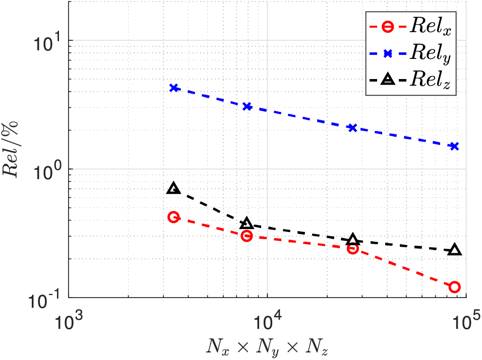
Figure 10: Displacement results for different node numbers

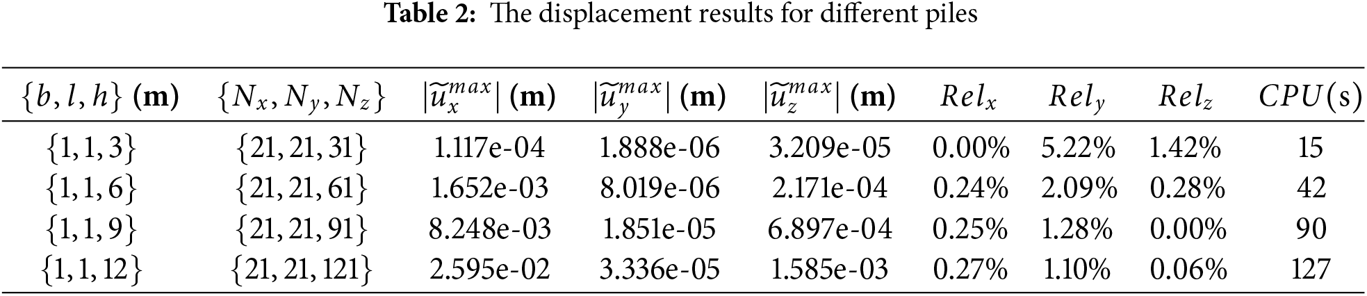
We further consider piles with different lengths, and the numerical results are shown in Table 2. The acceptable results for these four different sizes can be obtained by using the D-LRBFCM. We can infer that the D-LRBFCM could get acceptable outcomes if the parameters are chosen according to the above principles.

5.2 Example 2

An elastic-plastic problem is discussed to demonstrate the effectiveness of the mapping technique and incremental method. A 8 m × 4 m × 4 m soil slope is positioned on a rigid rock formation, and the soil deforms under gravity. The simplified mechanical state is shown in Fig. 11. The boundary conditions can be presented as follows:

Tx=0Pa,Ty=0Pa,Tz=0Pax=0m,ux=0m,Ty=0Pa,Tz=0Pax=8m,Tx=0Pa,uy=0m,Tz=0Pay=0m,Tx=0Pa,uy=0m,Tz=0Pay=4m,ux=0m,uy=0m,uz=0mz=0m,Tx=0Pa,Ty=0Pa,Tz=0Paz=4m.

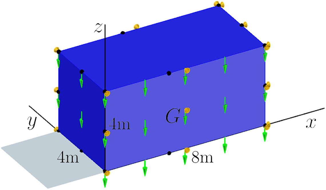
Figure 11: The mechanical state of Example 2

This example is essentially a plane strain problem, and uy is identically zero throughout the entire computational domain, so we only analyze numerical errors in ux and uz.

The displacement results of FEM are presented in Fig. 12 with |uxmax| = 1.128e-02 m and |uzmax| = 1.654e-02 m. The deformation primarily occurs at the inner side of the soil slope (side of x=0m); it is not economical or efficient to distribute the collocation nodes uniformly in the whole domain. By adjusting the locations of mapping seeds (the black ∙ in Fig. 11), most of the nodes can be concentrated on the inner side to better capture the displacement field variations, as shown in Fig. 13.

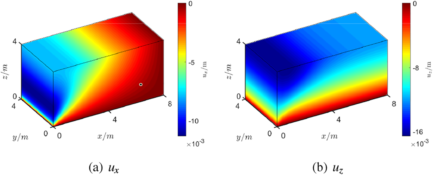
Figure 12: Displacement results of Example 2

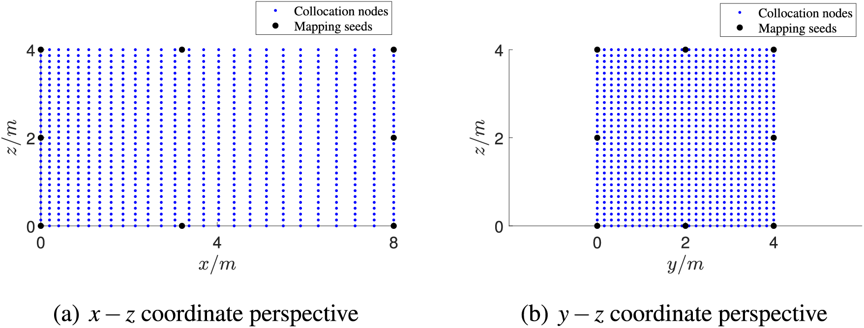
Figure 13: Node distribution in physical coordinate system

In the proposed method, we consider ns=3 and s=15. The results under different point arrays are shown in Fig. 14. We observe that we can obtain stable results for these different node arrays. As the number of points increases, the computation time increases continuously while the accuracy gradually improves and eventually stabilizes. The mapping technique can be effectively combined with D-LRBFCM for computation.

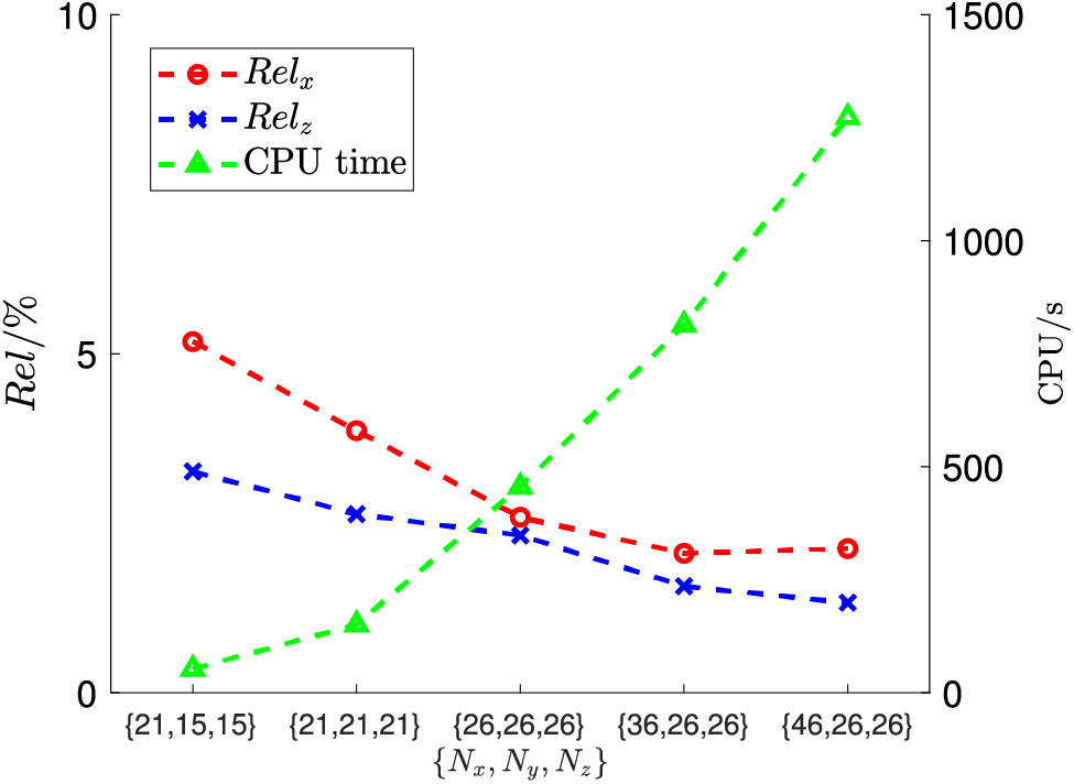
Figure 14: The accuracy of the D-LRBFCM under varying point arrays

Next, we use different incremental steps to calculate the elastic-plastic problem. The displacement solutions of the D-LRBFCM are shown in Fig. 15. As the number of steps s increases, the solutions of D-LRBFCM would converge and progressively align the FEM results. In this example, the results become relatively stable as the total steps exceed 15.

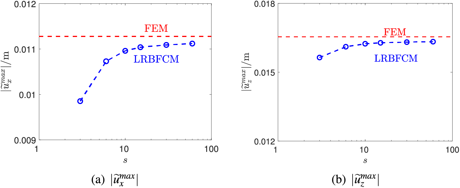
Figure 15: Displacement outcomes for various step numbers

5.3 Example 3

A rock-socketed excavation is analyzed in this example. The displacement of the rock formation under the soil layer is not considered, and the support structure is fixed in the rock. As shown in Fig. 16, there are 30 m × 15 m × 15 m soil layers located adjacent to the support structure on either side. The support structure is 1 m wide. The initial boundary conditions are defined as follows:

ux=0m,Ty=0Pa,Tz=0Pax=−31m,ux=0m,Ty=0Pa,Tz=0Pax=30m,Tx=0Pa,uy=0m,Tz=0Pay=0m,Tx=0Pa,uy=0m,Tz=0Pay=15m,ux=0m,uy=0m,uz=0mz=−15m,Tx=0Pa,Ty=0Pa,Tz=0Paz=0m.

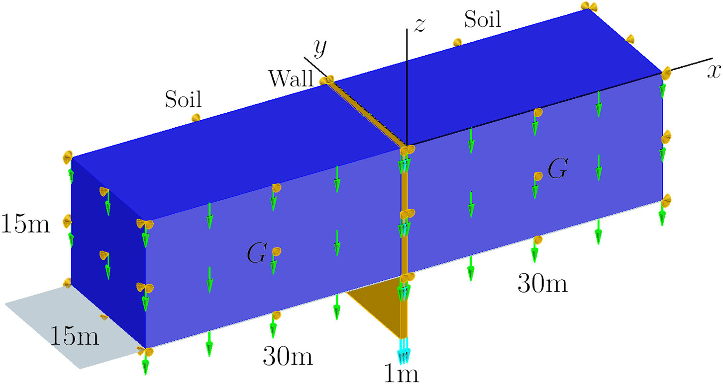
Figure 16: The prescribed mechanical state of Example 3

The excavation stress path can be categorized into three distinct stages, as illustrated in Fig. 17. The first stage is referred to as the geostatic equilibrium stage, which represents the soil deposition history. During this stage, the initial stresses of the structure reach equilibrate with the gravitational load of soil. However, the calculated deformations remain zero, since we are only concerned about the deformations after construction. The second stage is known as the support structure construction stage. The support wall is constructed and engages with the surrounding soil during this stage. The friction between the support structure and the soil is neglected, and the normal displacements of the contact surfaces are equal. The third stage, which is the one we are most concerned about, can be called the deformation stage. The passive soil located on the inner side of the excavation (x<−1 m) is removed, after which the active soil and the wall (x>0 m) start to deform together.

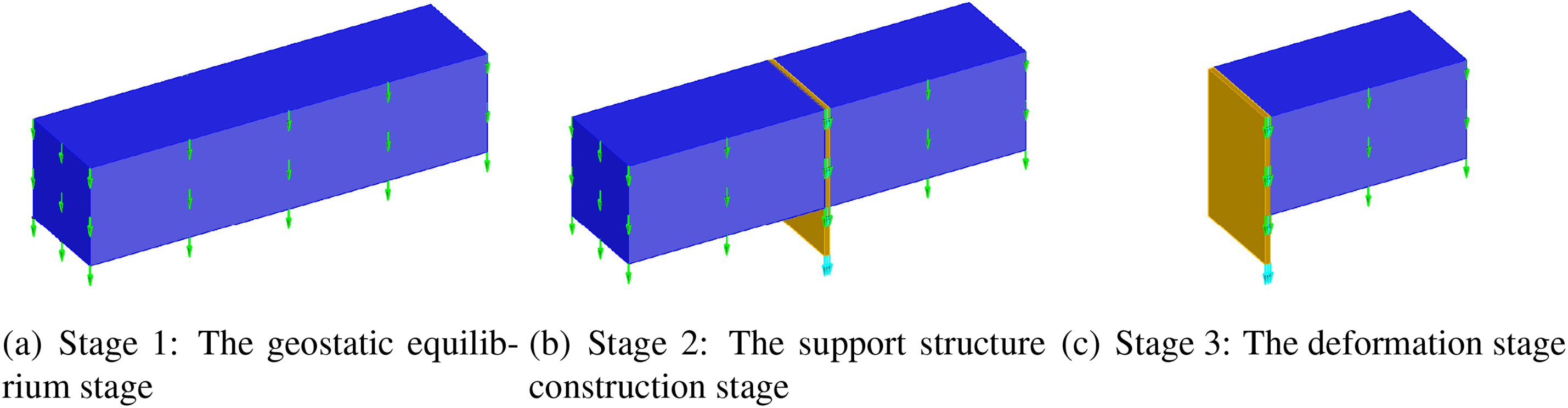
Figure 17: The stress path of excavation in Example 3

The final displacement solutions, as fielded through the FEM, are presented in Fig. 18 with |uxmax| = 9.960e-02 m and |uzmax| = 5.100e-02 m. For the proposed method, the mapping technique is used to optimize the node distribution. Fig. 19 shows the collocation node distribution in the physical coordinate system. s=15 is introduced. We employ three distinct node arrays to address the problem, and the results are summarized in Table 3. The results remain consistent across different node arrays, with the maximum value of relative error being 1.58%. The D-LRBFCM could get convincing solutions when we follow the principles outlined in the previous examples. In the FEM, we used the mesh with nodes arranged in the same distribution as the collocation points in D-LRBFCM and performed calculations with an equal number of incremental steps. The CPU times using the FEM software ABAQUS© are shown in Table 3. The results show that the D-LRBFCM is superior to FEM in terms of computational efficiency.

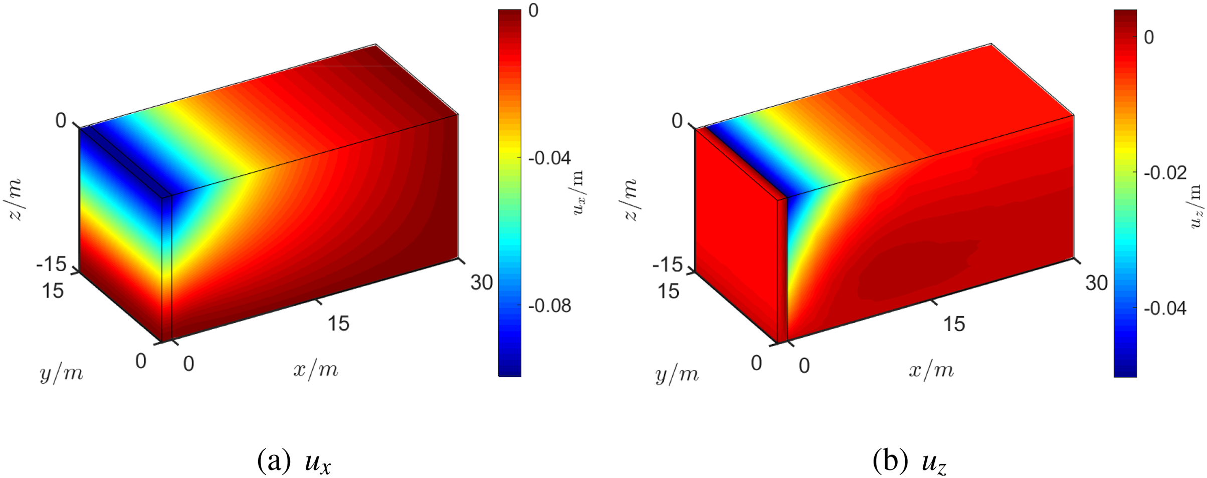
Figure 18: Displacement results of Example 3

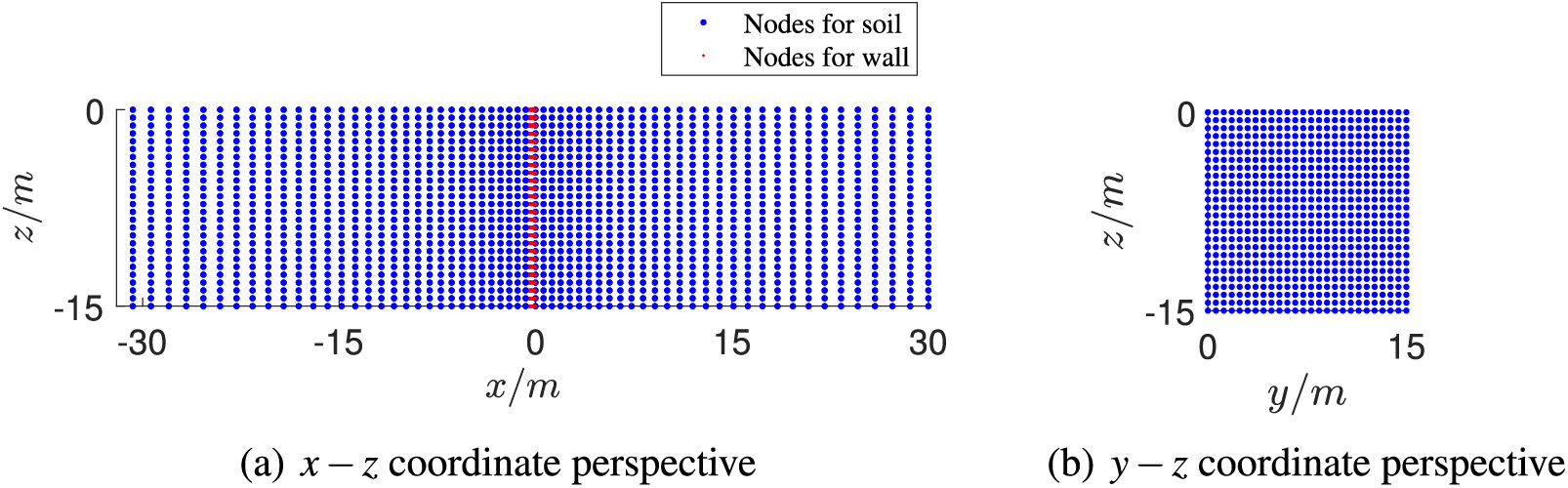
Figure 19: Node distribution for mapping technique

The work of applying the traditional LRBFCM in conjunction with the incremental method to solve similar excavation issues is also carried out. However, the results showed significant discretization. The reasons for this discretization are multifaceted: First, the large length-width ratio of the excavation support structure severely restricts the node distribution in the traditional LRBFCM, resulting in an unreasonable distribution of collocation points. Secondly, the presence of numerous first-order partial derivatives in the stress boundary conditions and governing equations makes it difficult to ensure accuracy. Furthermore, as verified in Example 1, the calculation accuracy of the traditional LRBFCM is quite sensitive to the shape parameter, which is difficult to determine. Therefore, Optimizing LRBFCM through the direct method is an essential step for simulating excavation deformation.

5.4 Example 4

In this example, we analyze a 3D rock-socketed circular excavation with a radius of 49 m. Considering the symmetry, we examine a quarter of the circle. As shown in Fig. 20, the excavation is 30 m deep, and the support wall is 1 m wide. The initial boundary conditions are:

ux=0m,Ty=0Pa,Tz=0Pax=0m,ux=0m,Ty=0Pa,Tz=0Pax=110m,Tx=0Pa,uy=0m,Tz=0Pay=0m,Tx=0Pa,uy=0m,Tz=0Pay=110m,ux=0m,uy=0m,uz=0mz=−30m,Tx=0Pa,Ty=0Pa,Tz=0Paz=0m.

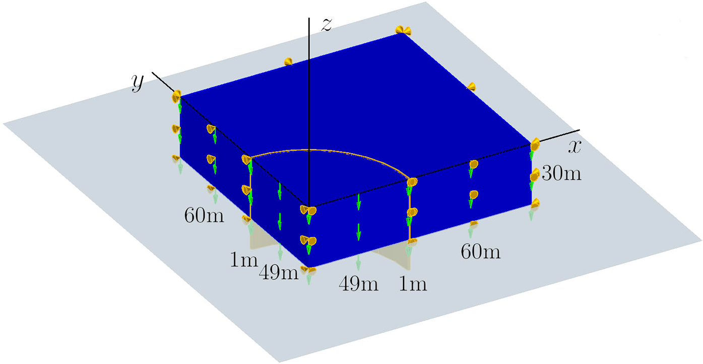
Figure 20: The prescribed mechanical state of Example 4

The friction between the soil and the support wall is ignored. Similarly to the previous example, the stress path consists of three stages (see Fig. 21). In the deformation stage, the passive soil within a radius of less than 49 m is excavated.

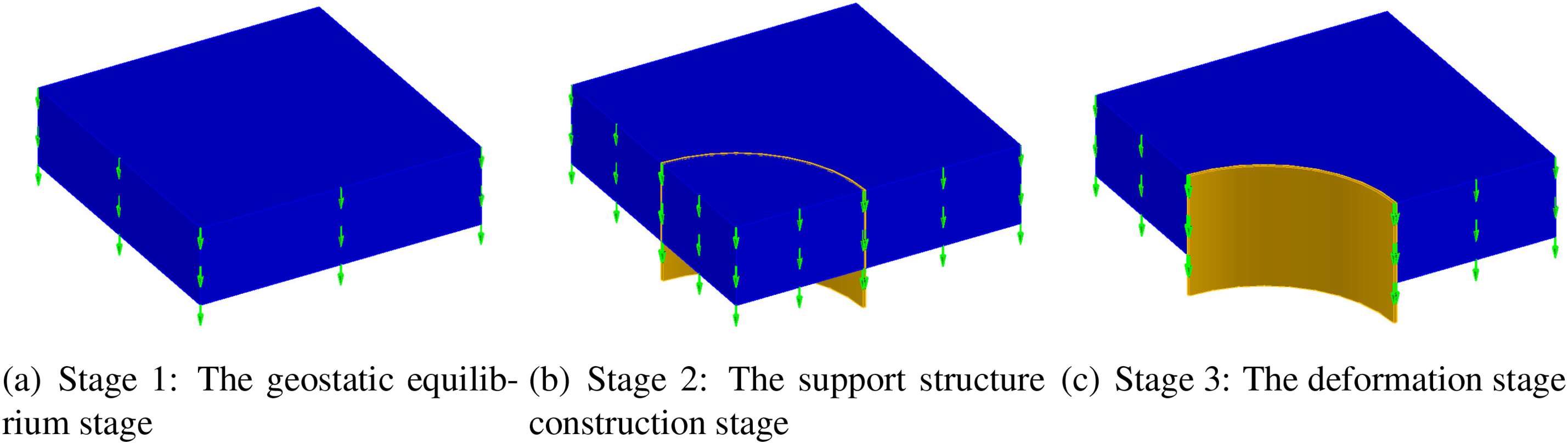
Figure 21: The stress path of excavation in Example 4

Considering the shape of the excavation, it needs to be divided into five blocks artificially, as shown in Fig. 22, for the mapping technique. The numbers in Fig. 22a represent the indices of the Blocks. In each block, an individual normalized coordinate system is constructed, and the collocation nodes are transformed to normalized nodes using the mapping seeds (the black ∙ in Fig. 22). The D-LRBFCM is applied in each block, respectively.

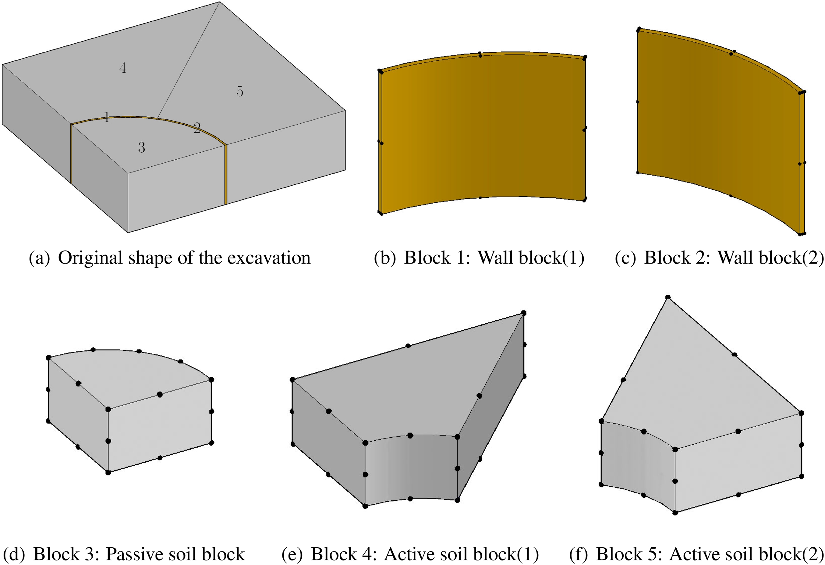
Figure 22: Dividing the excavation and collocating the mapping seeds

The final displacement solutions of FEM are shown in Fig. 23 with |uxmax| = 3.222e-02 m, |uymax| = 3.222e-02 m, and |uzmax| = 7.600e-03 m. The displacement fields of the 3D circular excavation differ from those of the strip excavation in Example 3. Firstly, the circular excavation can bear heavier soil weight and produce smaller deformation because of the circumferential hoop forces. At the same time, the plastic deformation of soil is significantly reduced. Secondly, the position of maximum lateral deformation of the support wall is changed. In Example 3, the top of the supporting wall has the largest deformation, whereas in the circular excavation, the maximum lateral displacement is located at the lower part of the wall. Lastly, the support wall in the circular excavation experiences a few positive displacements in the z-axis direction caused by the shell deflection (see Fig. 23c).

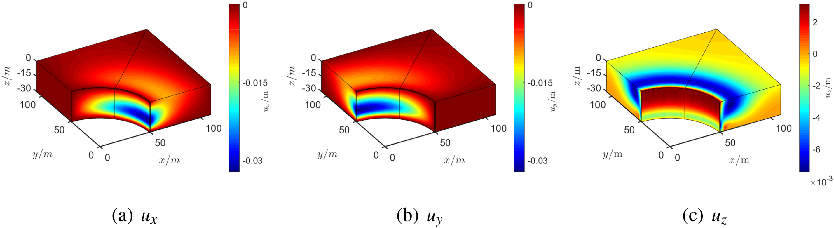
Figure 23: Displacement results of Example 4

For the proposed method, we consider s=15 and three different collocation node arrays, as shown in Table 4. The deformation results are presented in Table 5. The relative error values remain stable across the different node arrays, with the maximum error being 5.97%. A denser node array yields slightly better outcomes but also leads to lower computational efficiency.

5.5 Example 5

In the last example, a general circular excavation with a radius of 49 m is discussed. This model features an excavation within a 40 m deep soil region (see Fig. 24). The support wall has a thickness of 1 m, and the initial boundary conditions are as follows:

ux=0m,Ty=0Pa,Tz=0Pax=0m,ux=0m,Ty=0Pa,Tz=0Pax=110m,Tx=0Pa,uy=0m,Tz=0Pay=0m,Tx=0Pa,uy=0m,Tz=0Pay=110m,ux=0m,uy=0m,uz=0mz=−40m,Tx=0Pa,Ty=0Pa,Tz=0Paz=0m.

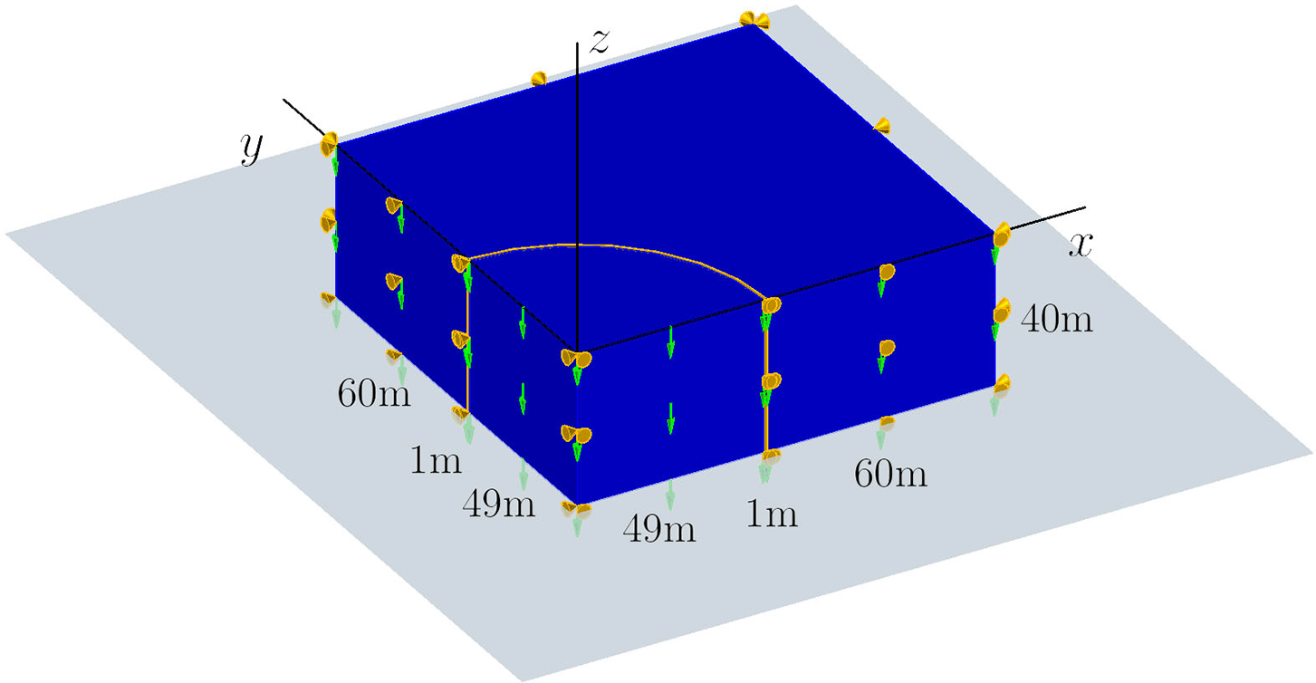
Figure 24: The prescribed initial boundary conditions for Example 5

We ignore the friction between the soil and the support wall. The stress path is also divided into three stages as shown in Fig. 25. During the deformation stage, the passive soil within R<49m, −20 m <z< 0 m is excavated. It means that there are three parts of the structure—the passive soil, the active soil and the support wall—working together, making the stress path more complex. This example is expected to be more difficult than the previous ones. Fig. 26 shows the final displacement solutions of FEM (|uxmax| = 3.544e-02 m, |uymax| = 3.544e-02 m and |uzmax| = 8.840e-03 m). It is important to note that there is a considerable upward movement in the passive soil, as the upper soil is excavated and its self-gravity is released. However, this deformation is generally not of concern in geotechnical engineering, and it is ignored in uz as shown in Fig. 26c.

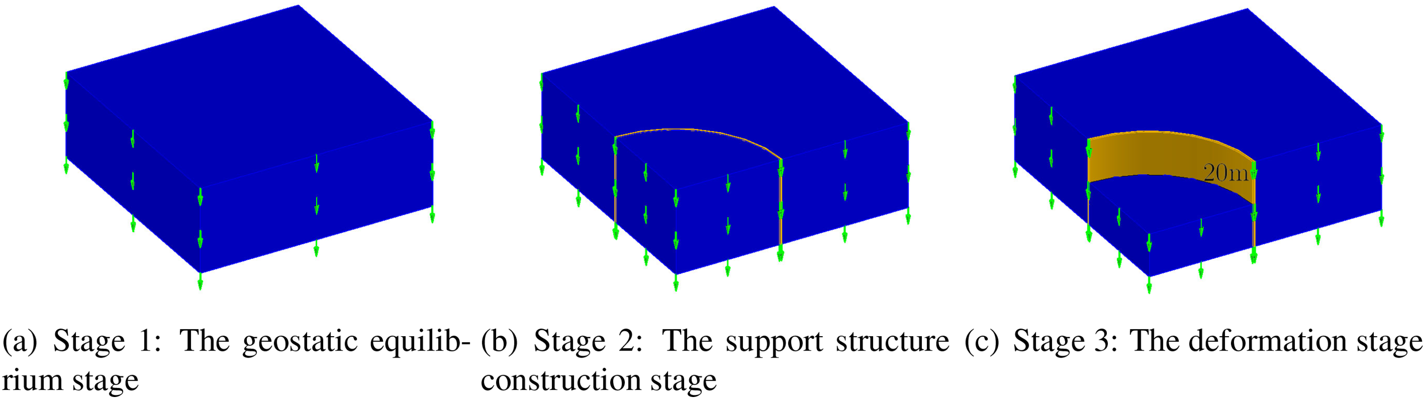
Figure 25: The stress path of excavation in Example 5

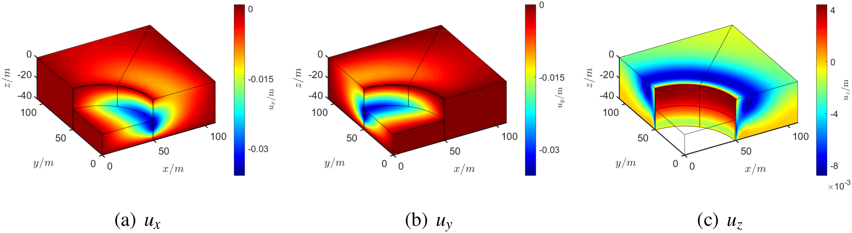
Figure 26: Displacement results of Example 5

Similarly to Example 4, the excavation shape is divided into five blocks artificially for the mapping technique, as shown in Fig. 27, where the indices of blocks are presented. We build an individual normalized coordinate system for each block. Tables 6 and 7 show the results of three different node arrays. Compared with the other examples, this problem is more complex, and the accuracy is slightly inferior but still acceptable. The results also show that a denser node array yields slightly better accuracy.

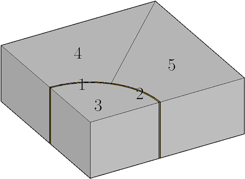
Figure 27: Dividing the excavation and the indices of blocks of Example 5

6  Conclusions

This paper extends the LRBFCM to the deformation analysis of deep excavation in 3D. The direct method, where the influence nodes are collocated on a straight line, is introduced to optimize the local nodes. The mapping technique is used to describe the irregular shape of excavation in 3D. The plasticity of soil in excavation is described by the D-P model, and the LRBFCM, using the incremental method, is applied to analyze the plasticity. The efficiency of modified LRBFCM is demonstrated through five examples. By using the proposed optimization methods, LRBFCM can effectively solve deep excavation problems. The following conclusions can be made:

1.    The application of the direct method is crucial for simulating excavation deformation. By using the direct method, the accuracy of computing first-order partial derivatives is significantly improved. Additionally, the collocation node distribution can be adjusted flexibly, greatly enhancing the computational efficiency when solving significant length-width ratio problems. Moreover, the direct method is insensitive to the shape parameter, making the calculation more stable.

2.    The shape of circular excavation can be described with several quadratic-type blocks, and the deformation results remain stable since the physical coordinates are transformed into a normalized coordinate system.

3.    A suitable range of 10<cx/dx,cy/dy,cz/dz<14,000 is recommended for the D-LRBFCM when solving 3D deep excavation problems.

4.    Compared to the strip excavation, the plastic deformation of soil in a circular excavation is significantly reduced, and the position of maximum lateral deformation shifts from the top to the lower part of the wall.

Our current study exclusively addresses the problem of single-layer soil, and our future work will focus on multi-layer soils and inhomogeneous materials. Additionally, large deformation problems in geotechnical engineering may also be considered in future studies.

Acknowledgment: The authors would like to acknowledge China Scholarship Council (CSC) for its support on this study.

Funding Statement: The work was supported by grants from the National Natural Science Foundation of China (Nos. 12172159 and 12362019).

Author Contributions: The authors confirm contribution to the paper as follows: study conception and design: Cheng Deng, Liangyong Gong; data collection: Rongping Zhang, Mengqi Wang; analysis and interpretation of results: Cheng Deng, Hui Zheng, Liangyong Gong, Rongping Zhang; draft manuscript preparation: Cheng Deng, Hui Zheng, Mengqi Wang. All authors reviewed the results and approved the final version of the manuscript.

Availability of Data and Materials: The data presented in this study are available on request from the corresponding author.

Ethics Approval: Not applicable.

Conflicts of Interest: The authors declare no conflicts of interest to report regarding the present study.

References

1. Zhang J, Li M, Ke L, Yi J. Distributions of lateral earth pressure behind rock-socketed circular diaphragm walls considering radial deflection. Comput Geotech. 2022;143(4):104604. doi:10.1016/j.compgeo.2021.104604. [Google Scholar] [CrossRef]

2. Zhou X, Yuan Y, Leng Z, Gao X, Zeng C. Numerical study on the thermal-induced mechanical behavior in deep energy diaphragm wall (EDWthe long-term soil elastoplastic effects. Tunn Undergr Sp Tech. 2023;132:104860. doi:10.1016/j.tust.2022.104860. [Google Scholar] [CrossRef]

3. Lai VQ, Kounlavong K, Keawsawasvong S, Banyong R, Wipulanusat W, Jamsawang P. Undrained basal stability of braced circular excavations in anisotropic and non-homogeneous clays. Transp Geotech. 2023;39(2):100945. doi:10.1016/j.trgeo.2023.100945. [Google Scholar] [CrossRef]

4. Kumar J, Rahaman O. Lower bound limit analysis of unsupported vertical circular excavations in rocks using Hoek-Brown failure criterion. Int J Numer Anal Met. 2020;44(7):1093–106. doi:10.1002/nag.3051. [Google Scholar] [CrossRef]

5. Drucker DC, Prager W. Soil mechanics and plastic analysis or limit design. Q Appl Math. 1952;10(2):157–65. doi:10.1090/qam/48291. [Google Scholar] [CrossRef]

6. Zhu XH, Jia YJ. 3D mechanical modeling of soil orthogonal cutting under a single reamer cutter based on Drucker-Prager criterion. Tunn Undergr Sp Tech. 2014;41:255–62. doi:10.1016/j.tust.2013.12.008. [Google Scholar] [CrossRef]

7. He W, Luo C, Cui J, Zhang J. An axisymmetric BNEF method of circular excavations taking into account soil-structure interactions. Comput Geotech. 2017;90(11):155–63. doi:10.1016/j.compgeo.2017.06.001. [Google Scholar] [CrossRef]

8. Keawsawasvong S, Ukritchon B. Undrained basal stability of braced circular excavations in non-homogeneous clays with linear increase of strength with depth. Comput Geotech. 2019;115(2):103180. doi:10.1016/j.compgeo.2019.103180. [Google Scholar] [CrossRef]

9. Arai Y, Kusakabe O, Murata O, Konishi S. A numerical study on ground displacement and stress during and after the installation of deep circular diaphragm walls and soil excavation. Comput Geotech. 2008;35(5):791–807. doi:10.1016/j.compgeo.2007.11.001. [Google Scholar] [CrossRef]

10. Wang D, Bienen B, Nazem M, Tian Y, Zheng J, Pucker T, et al. Large deformation finite element analyses in geotechnical engineering. Comput Geotech. 2015;65(13):104–14. doi:10.1016/j.compgeo.2014.12.005. [Google Scholar] [CrossRef]

11. Zheng H, Yang Z, Zhang C, Tyrer M. A local radial basis function collocation method for band structure computation of phononic crystals with scatterers of arbitrary geometry. Appl Math Model. 2018;60(13):447–59. doi:10.1016/j.apm.2018.03.023. [Google Scholar] [CrossRef]

12. Cheng AHD, Hong Y. An overview of the method of fundamental solutions—Solvability, uniqueness, convergence, and stability. Eng Anal Bound Elem. 2020;120(5):118–52. doi:10.1016/j.enganabound.2020.08.013. [Google Scholar] [CrossRef]

13. Chen W, Tanaka M. A meshless, integration-free, and boundary-only RBF technique. Comput Math Appl. 2002;43(3):379–91. doi:10.1016/S0898-1221(01)00293-0. [Google Scholar] [CrossRef]

14. Wang F, Gu Y, Qu W, Zhang C. Localized boundary knot method and its application to large-scale acoustic problems. Comput Method Appl M. 2020;361:112729. doi:10.1016/j.cma.2019.112729. [Google Scholar] [CrossRef]

15. Gu Y, Lin J, Fan CM. Electroelastic analysis of two-dimensional piezoelectric structures by the localized method of fundamental solutions. Adv Appl Math Mech. 2023;15(4):880–900. doi:10.4208/aamm.OA-2021-0223. [Google Scholar] [CrossRef]

16. Sarler B, Vertnik R. Meshfree explicit local radial basis function collocation method for diffusion problems. Comput Math Appl. 2006;51(8):1269–82. doi:10.1016/j.camwa.2006.04.013. [Google Scholar] [CrossRef]

17. Vertnik R, Sarler B. Meshless local radial basis function collocation method for convective-diffusive solid-liquid phase change problems. Int J Numer Method Heat Fluid Flow. 2006;16(5):617–40. doi:10.1108/09615530610669148. [Google Scholar] [CrossRef]

18. Jiang P, Zheng H, Xiong J, Zhang C. A stabilized local RBF collocation method for incompressible Navier-Stokes equations. Comput Fluids. 2023;265(3):105988. doi:10.1016/j.compfluid.2023.105988. [Google Scholar] [CrossRef]

19. Tu W, Gu YT, Wen PH. Effective shear modulus approach for two dimensional solids and plate bending problems by meshless node collocation method. Eng Anal Bound Elem. 2012;36(5):675–84. doi:10.1016/j.enganabound.2011.11.016. [Google Scholar] [CrossRef]

20. Zhang S. Meshless symplectic and multi-symplectic local RBF collocation methods for nonlinear Schrodinger equation. J Comput Phys. 2022;450(2):110820. doi:10.1016/j.jcp.2021.110820. [Google Scholar] [CrossRef]

21. Xue Z, Wang L, Ren X, Wahab MA. Weighted radial basis collocation method for large deformation analysis of rubber-like materials. Eng Anal Boundary Elem. 2023;159:95–110. doi:10.1016/j.enganabound.2023.11.016. [Google Scholar] [CrossRef]

22. Chen C, Noorizadegan A, Young DL, Chen CS. On the selection of a better radial basis function and its shape parameter in interpolation problems. Appl Math Comput. 2023;442(1):127713. doi:10.1016/j.amc.2022.127713. [Google Scholar] [CrossRef]

23. Rippa S. An algorithm for selecting a good value for the parameter c in radial basis function interpolation. Adv Comput Math. 1999;11(2–3):193–210. doi:10.1023/A:1018975909870. [Google Scholar] [CrossRef]

24. Franke R. Scattered data interpolation: tests of some methods. Math Comput. 1982;38(157):181–200. doi:10.2307/2007474. [Google Scholar] [CrossRef]

25. Shi CS, Zheng H, Wen PH, Hon YC. The local radial basis function collocation method for elastic wave propagation analysis in 2D composite plate. Eng Anal Bound Elem. 2023;150(1–2):571–82. doi:10.1016/j.enganabound.2023.02.021. [Google Scholar] [CrossRef]

26. Xu Y, Li J, Chen X, Pang G. Solving fractional Laplacian Visco-acoustic wave equations on complex-geometry domains using Grunwald-formula based radial basis collocation method. Comput Math Appl. 2020;79(8):2153–67. doi:10.1016/j.camwa.2019.10.013. [Google Scholar] [CrossRef]

27. Wang D, Chen CS, Fan CM. The MAPS based on trigonometric basis functions for solving elliptic partial differential equations with variable coefficients and Cauchy-Navier equations. Math Comput Simulat. 2019;159(8/9):119–35. doi:10.1016/j.matcom.2018.11.001. [Google Scholar] [CrossRef]

28. Li M, Wen PH. Finite block method for transient heat conduction analysis in functionally graded media. Int J Numer Meth Eng. 2014;99(5):372–90. doi:10.1002/nme.4693. [Google Scholar] [CrossRef]

29. Wen PH, Cao P, Korakianitis T. Finite block method in elasticity. Eng Anal Bound Elem. 2014;46(4):116–25. doi:10.1016/j.enganabound.2014.05.006. [Google Scholar] [CrossRef]

30. Wen JC, Zhou YR, Zhang CG, Wen PH. Meshless variational method applied to fracture mechanics with functionally graded materials. Eng Anal Bound Elem. 2023;157(2):44–58. doi:10.1016/j.enganabound.2023.08.043. [Google Scholar] [CrossRef]

31. Wen JC, Zhou YR, Sladek J, Sladek V, Wen PH. Galerkin finite block method in solid mechanics. Comput Math Appl. 2024;155(2):66–79. doi:10.1016/j.camwa.2023.11.028. [Google Scholar] [CrossRef]

32. Owen DRJ, Hinton E. Finite elements in plasticity: theory and practice. Swansea, UK: Pineridge Press Limited; 1980. [Google Scholar]

33. Abbo AJ, Sloan SW. A smooth hyperbolic approximation to the Mohr-Coulomb yield criterion. Comput Struct. 1995;54(3):427–41. doi:10.1016/0045-7949(94)00339-5. [Google Scholar] [CrossRef]