
 Submit a Paper
 Propose a Special lssue
 Open Access
ARTICLE

A Study of the 1 + 2 Partitioning Scheme of Fibrous Unitcell under Reduced-Order Homogenization Method with Analytical Influence Functions
1 HEDPS, Center for Applied Physics and Technology (CAPT), Department of Mechanics and Engineering Science, College of Engineering, Peking University, Beijing, 100871, China
2 State Key Laboratory for Turbulence and Complex Systems, Peking University, Beijing, 100871, China
* Corresponding Author: Zifeng Yuan. Email:
Computer Modeling in Engineering & Sciences 2025, 142(3), 2893-2924. https://doi.org/10.32604/cmes.2025.059948
Received 21 October 2024; Accepted 21 January 2025; Issue published 03 March 2025
 View Full Text
 Download PDF
Abstract
The multiscale computational method with asymptotic analysis and reduced-order homogenization (ROH) gives a practical numerical solution for engineering problems, especially composite materials. Under the ROH framework, a partition-based unitcell structure at the mesoscale is utilized to give a mechanical state at the macro-scale quadrature point with pre-evaluated influence functions. In the past, the “1-phase, 1-partition” rule was usually adopted in numerical analysis, where one constituent phase at the mesoscale formed one partition. The numerical cost then is significantly reduced by introducing an assumption that the mechanical responses are the same all the time at the same constituent, while it also introduces numerical inaccuracy. This study proposes a new partitioning method for fibrous unitcells under a reduced-order homogenization methodology. In this method, the fiber phase remains 1 partition, but the matrix phase is divided into 2 partitions, which refers to the “1 + 2” partitioning scheme. Analytical elastic influence functions are derived by introducing the elastic strain energy equivalence (Hill-Mandel condition). This research also obtains the analytical eigenstrain influence functions by alleviating the so-called “inclusion-locking” phenomenon. In addition, a numerical approach to minimize the error of strain energy density is introduced to determine the partitioning of the matrix phase. Several numerical examples are presented to compare the differences among direct numerical simulation (DNS), “1 + 1”, and “1 + 2” partitioning schemes. The numerical simulations show improved numerical accuracy by the “1 + 2” partitioning scheme.Keywords
Fibrous composite materials with the advantages of high specific strength, specific stiffness, and corrosion resistance are widely used in many advanced manufacturing sectors, and that leads to the demand for high-fidelity evaluation of mechanical properties of the composite structures [1–3]. However, the overall mechanical response of composite materials is complicated because of the large gap between the mechanical properties of each constituent, especially when the nonlinearities are considered. The various mesoscale geometric structures of fibrous composite materials and loading patterns also lead to different types of material failure, such as breakage of fibers, debonding of fiber/matrix interface, or delamination of plies. Therefore, developing an efficient framework for the constitutive model of composite materials with comprehensive consideration of various nonlinear material behaviors is important, and a series of research has been conducted in this area. Firstly, various homogenized anisotropic damage models of the composite material were proposed [4–6] and applied in engineering. Meanwhile, based on the high-resolution modeling, many investigations were conducted to capture the failure mechanism on the mesoscale [7–9]. In these homogenized damage models, the loss of microscale information usually leads to a loss of accuracy and generalizability; the increasing complexity of the homogenized model also requires extensive calibration. On the other hand, the orders of magnitude gap between the characteristic length of the mesoscale model and composite structure gives rise to unacceptable computation costs. Therefore, the so-called multiscale method based on continuum mechanics, also labeled as an upscaling method, has been developed rapidly to balance fidelity and computation efficiency. A series of works on direct multiscale methods, such as the multilevel finite element (
Transformation field analysis (TFA) is a typical reduced model proposed by Dvorak for the analysis of elastic composite [13] and then extended for the inelastic cases [14]. The scale transitions of strain and stress in heterogeneous structures were expressed explicitly by this approach, where plastic strain and thermal expansion were treated as eigenstrain. In TFA, the transformation influence functions and concentration factors are precomputed based on the mechanical parameters of different phases and the geometric structure of the composite. The number of variables was reduced significantly due to the assumption of piecewise uniform fields. Therefore, this approach was utilized and developed for the analyses of composite structures by many scholars over the past three decades [15–17]. However, some deficiencies of classical TFA were recognized in practice. First, the prediction of macroscopic stress is usually too stiff due to the assumption of piecewise uniform plastic strain [18,19]. In addition, expectedly, the accuracy of the two-phase system in inelastic analysis is unsatisfactory when following the principle of so-called “1-phase-1-partition”. That leads to the finer division of each individual phase, in other words, a larger number of internal variables in overall constitutive relations [20]. Instead of finer division in the space domain of each phase, decomposing the plastic strain into a finite combination set of plastic modes, the so-called nonuniform transformation field analysis (NTFA) [21,22], is another option for reaching higher precision. However, the extra work for calibrating empirical laws and extensive exploration of the deformation space under plastic deformation can counteract the advantage of NTFA on computational efficiency.
Liu et al. proposed the self-consistent clustering analysis (SCA) method [23] to overcome the limitations of TFA and its derivatives. In the SCA method, the constituents of composites are divided into a specific number of subdomains by
Other machine learning-based multiscale techniques have also been developed as an important direction of model reduction. Zhang et al. [37] developed a reduced-order model of the hierarchical deep-learning neural networks (HiDeNN) based on a tensor decomposition (TD). A reduced-order machine learning finite element method based on proper generalized decomposition (PGD) reduced HiDeNN presents a good performance in the multiscale analysis of composite materials, topology optimization, and additive manufacturing [38]. Fish et al. [39,40] proposed a data-physics-driven reduced-order homogenization (dpROH) approach, which significantly improves the accuracy of physics-based reduced-order homogenization (pROH) by combining data generated from high-fidelity models with Bayesian inference. The artificial neural network (ANN) and deep material network (DMN) were also applied to homogenize the nonlinear mechanical properties of heterogeneous materials [41,42]. Masrouri et al. [43] utilized generative AI to predict the stress distribution of bicontinuous composites with complex irregular distribution.
The motivation of the present work is to develop a reduced-order homogenization (ROH) multiscale method [44–47] for fibrous composite material, in which the overestimation of strength due to “1-phase-1-partition” is improved while no extra internal variables of the constitutive model of each phase are introduced; in addition, simple and explicit partitioning of the subdomains of constituents is preferred over to the complicated and implicit partitioning of cluster-discretization methods. Therefore, a framework of constitutive model based on the ROH method is proposed, in which an adaptive method for partitioning the matrix phase is involved. This model can capture the stress concentration on the mesoscale and predict the overall response of fibrous composite with better precision since the matrix phase is divided into inner and outer matrix partitions with an independent nonlinear evolution process. The volume fraction of the inner matrix partition is predicted by a numerical calculation method, whose object function targets the minimization of error in strain energy density compared to the results from a modified Eshelby method [48–51]. In addition, the influence functions of elastic strain and eigenstrain are calculated analytically so that the offline computation is simplified drastically. In this manuscript, the framework of reduced-order homogenization is briefly introduced in Section 2; the mathematical manipulation of the analytical solution of influence functions for 1 + 2 partitions is presented in Section 3, along with the numerical calculation method for partitioning of the matrix phase; the numerical results for the verification of new model under different volume fractions of fiber are exhibited in Section 4; finally, the discussion of the numerical results and the corresponding conclusions are provided in Sections 5 and 6, respectively.
2 Reduced-Order Homogenization
The multiscale computational homogenization method based on the unitcell discretized by finite elements is usually computationally prohibitive for general macroscopic structures. It requires averaging and homogenization procedures over a converged unitcell problem at every macroscopic integration point during each Newton-Raphson iteration. In addition, the unitcell problem involving material nonlinearities needs to be solved using a Newton-Raphson iterative method. Model reduction technique is necessary to reduce the degrees of freedom by applying a specific distribution of mechanical response over phases at the mesoscale. The reduced-order homogenization (ROH) approach is a typical multiscale method with low computational cost, adopting a piecewise constant approximation of mechanical quantities over each partition.
In addition, the concept of eigenstrain is introduced to consider the material nonlinear response that
where
where
The elastic strain influence functions satisfy the following two constraints:
A two-partition unitcell model can be used for a general inclusion-matrix heterogeneous material under the assumption that each phase material always keeps the same response. Thus, it significantly reduces computational costs compared to the so-called direct-homogenization.
3 Fibrous Unitcell with 1 + 2 Partitions
The “1-phase-1-partition” reduced-order homogenization (ROH) method significantly decreases computational cost. However, under general multi-axial deformation, the distribution of material status within one phase is not uniform, which can give a stiffer material response than the direct-homogenization method due to the over-constraint of the material points. This study takes a fibrous unitcell as an example, as depicted in Fig. 1, and the matrix phase is partitioned into the inner and outer partitions. It visualizes the stress distribution under different loading modes, including uniaxial tension in longitudinal (Fig. 2a,b) and transverse (Fig. 2e,f) directions, shear in the longitudinal-transverse plane (Fig. 2c,d) and transverse plane (Fig. 2g,h). These numerical results show different stress magnitudes between the inner and outer partitions at the matrix phase.
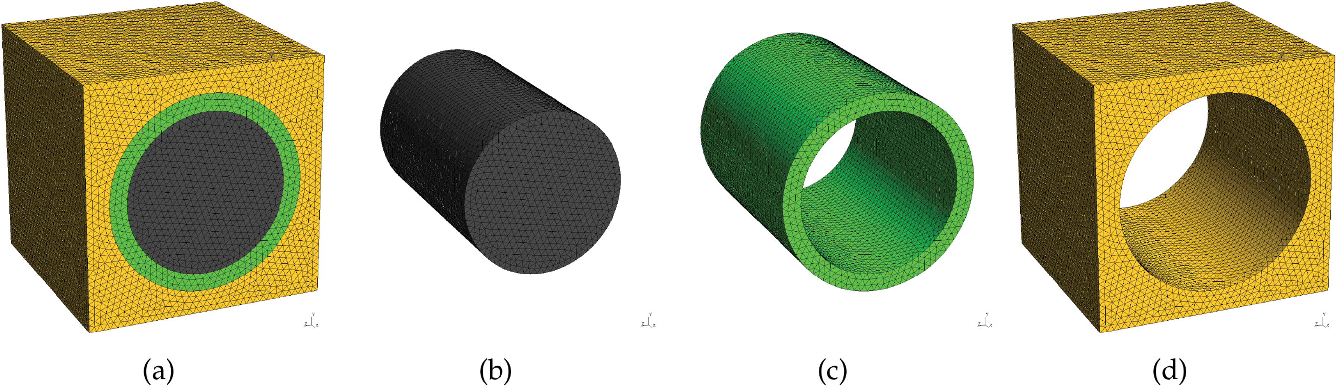
Figure 1: A sketch of a three-partition fibrous unitcell with finite element discretization: (a) fibrous unitcell; (b) fiber phase; (c) inner matrix partition; and (d) outer matrix partition
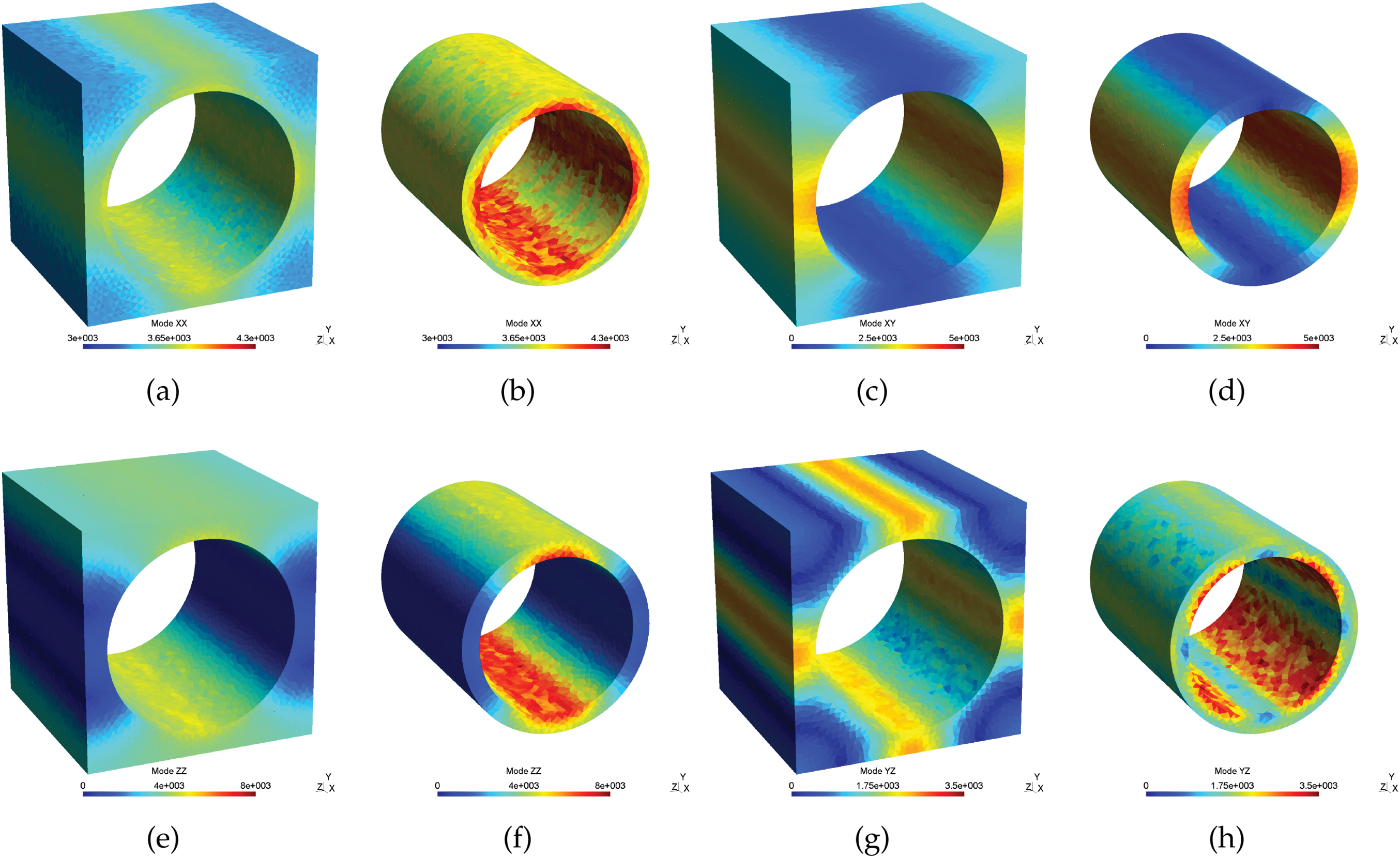
Figure 2: A sketch of von Mises stress of 1st and 2nd matrix partition under different loading modes: (a and b) uniaxial tension along the longitudinal direction; (c and d) simple shear at the longitudinal-transverse plane; (e and f) uniaxial tension along the transverse direction; and (g and h) simple shear at the transverse plane
This study uses the ROH method for the fibrous unitcell with two partitions at the matrix phase. We define this partition as a “1 + 2” partition. Due to the transverse isotropy symmetry of fibrous composite material, this study divided the matrix phase into the inner and outer partitions, as depicted in Fig. 1c,d, respectively. In the rest of the paper, the properties and status associated with the fiber phase, matrix phase, inner matrix partition, outer matrix partition, unitcell (mesoscale), and coarse (macroscopic) scale are denoted as
3.1 Elastic Strain Influence Functions
From the point of view of macroscopic elastic strain energy density, the following can be obtained:
On the other hand, the mesoscale partitions give the elastic strain energy density that
Under elastic response, the averaged strains at partitions are given as follows:
Substituting (9) into (8) yields
Comparing (7) and (10) and asking for
In addition, recall the equations for the elastic strain influence functions (3) and (4) for the fibrous unitcell that
In addition, define
so that
Rearranging (18) yields
Similarly, substituting (17) into (16) and eliminating
The right-hand-side term in (19) and (20) can be proved as semi-positive-definite. The proof is given in Appendix A. Suppose
where
For any macroscopic strain
Due to the positive definiteness of
where
where
3.2 Eigenstrain Influence Functions
For the fibrous unitcell with 1 + 2 partitions, the reduced-order system of equations is derived from (2) that
The eigenstrain influence tensors satisfy the following constraints (Chapter 4 of the textbook [52]):
This constructs two special cases with perfect plastic yielding at selected partition(s) to solve the eigenstrain influence functions. For Case I, it asks that the outer partition of the matrix gets perfect plastic yielding while the inner partition of the matrix and the fiber phase remain elastic. For Case II, it assumes that the whole matrix phase gets perfect plastic yield while the fiber is still elastic. A sketch of two cases is depicted in Fig. 3.
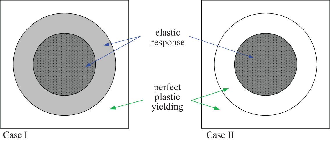
Figure 3: Sketch of two cases with perfect plastic yielding at selected partition(s)
In the first case, under macroscopic strain
The derivation of the vector components can be seen in Appendix C.
Thus, it can define the so-called perfect plastic influence function for the fiber phase and the inner partition of the matrix phase that
and
For the fiber-dominated mode, i.e., the longitudinal direction,
with
The sub-matrix
with the arbitrariness of
Once the perfect plastic influence functions for all partitions are determined, the eigenstrain influence functions
From (45), it can find
Through (43) and (44), it can obtain
and
respectively.
Case II is studied, where the whole matrix phase gets perfect plastic yield while the fiber is still elastic. Similarly, under macroscopic strain
Thus, it can define the perfect plastic influence function for the fiber phase and the inner partition of the matrix phase that
and
The strain influence function for the outer partition of the matrix phase is first written as follows:
For the fiber-dominated mode, i.e., the longitudinal direction,
with
The sub-matrix
with the arbitrariness of
3.3 Volume Fraction of Inner and Outer Matrix Partitions
The purpose of searching for the optimum volume fraction of inner matrix partition
where
Then (64) yields
The average
Therefore, the optimum inner matrix partition volume fraction can be calculated by solving the following equation numerically to obtain the extreme point of
This study investigates the nonlinear behaviors of the fibrous composite due to transverse loadings and chooses the following macroscopic strain loading space to search the optimum
where
and
The average strain energy densities of inner and outer matrix partitions under a given global strain loading
Since the integrals of
where
Then (66) can be written as follows:
while
After solving (66) numerically, the optimum
This section predicts the optimum volume fractions of inner matrix partition
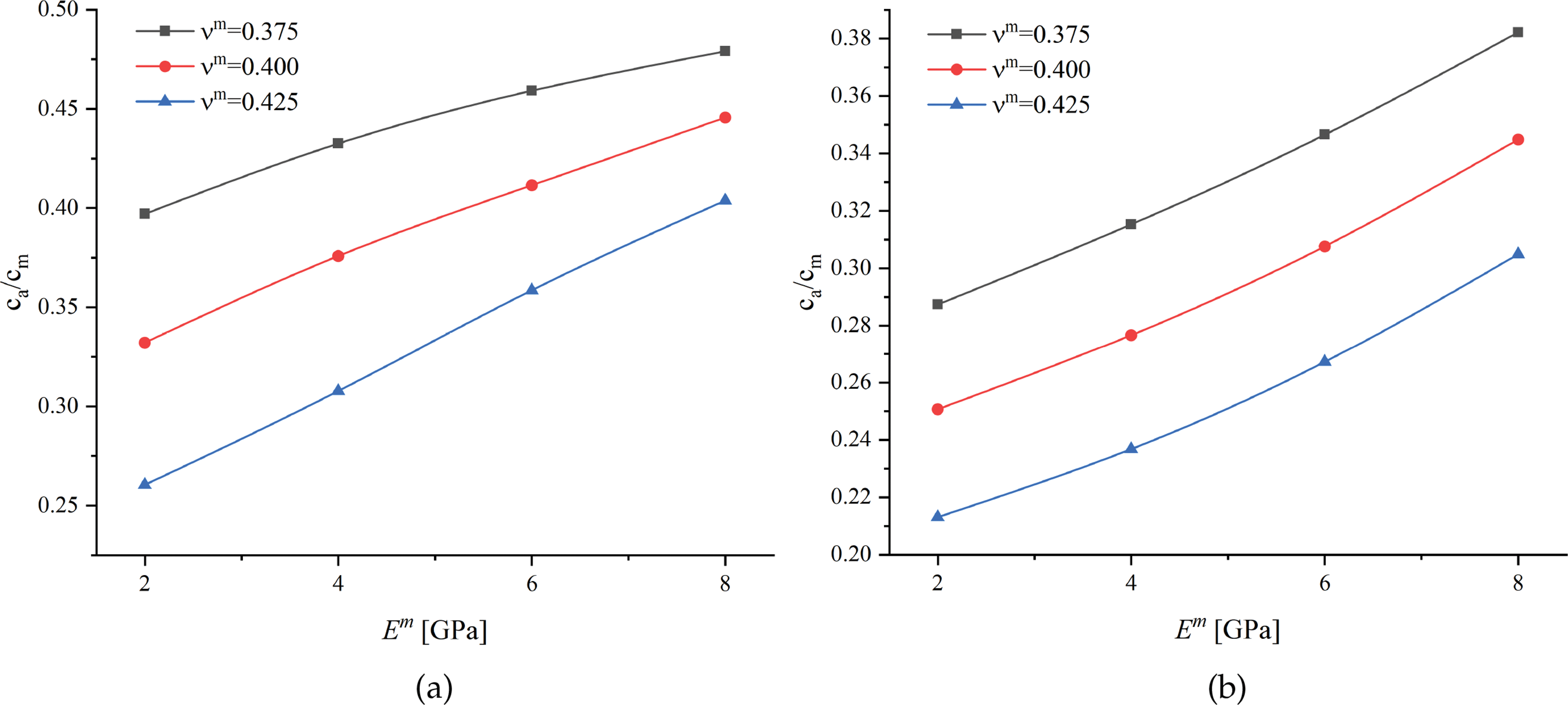
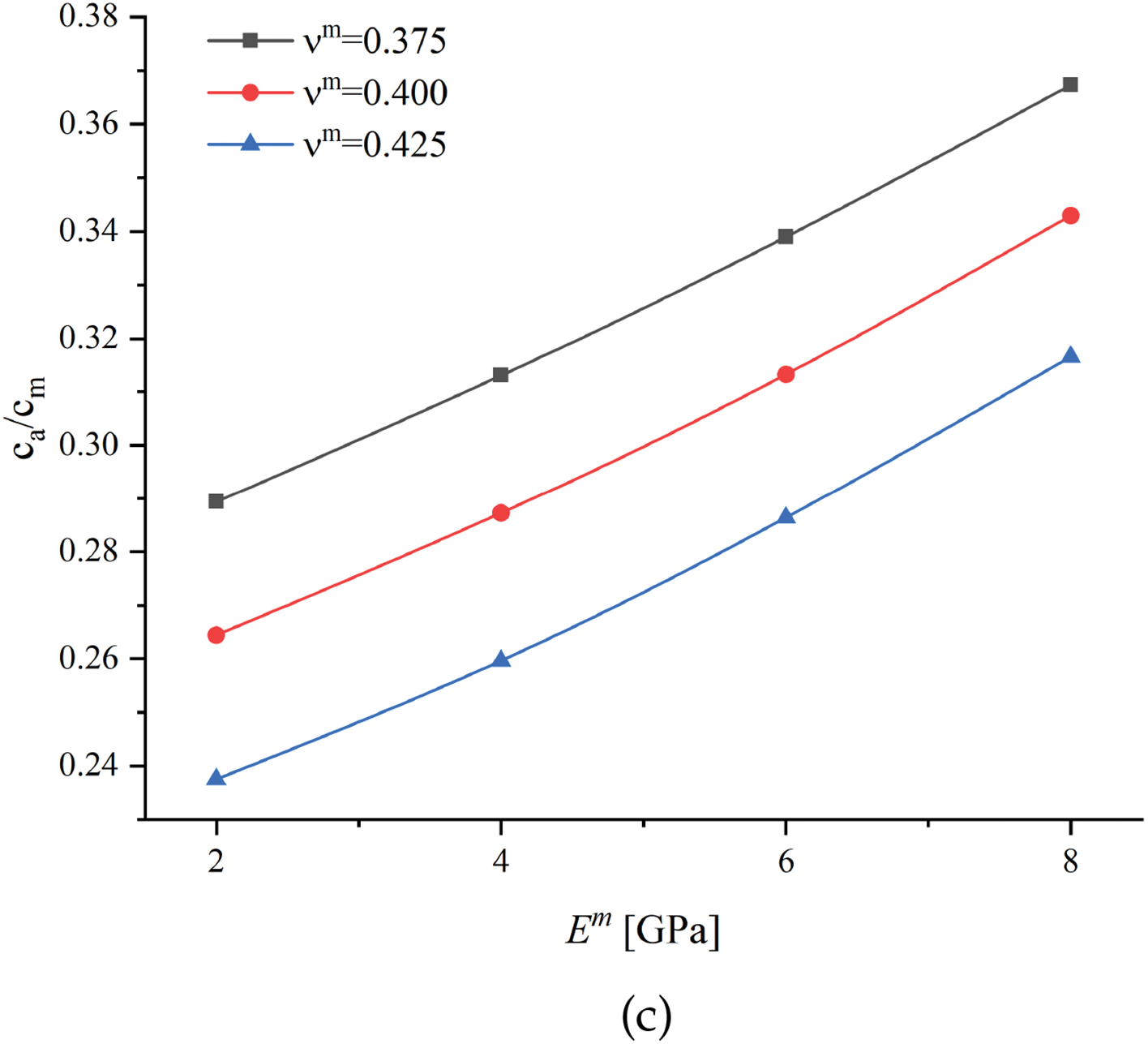
Figure 4: Numerical relative volume fraction
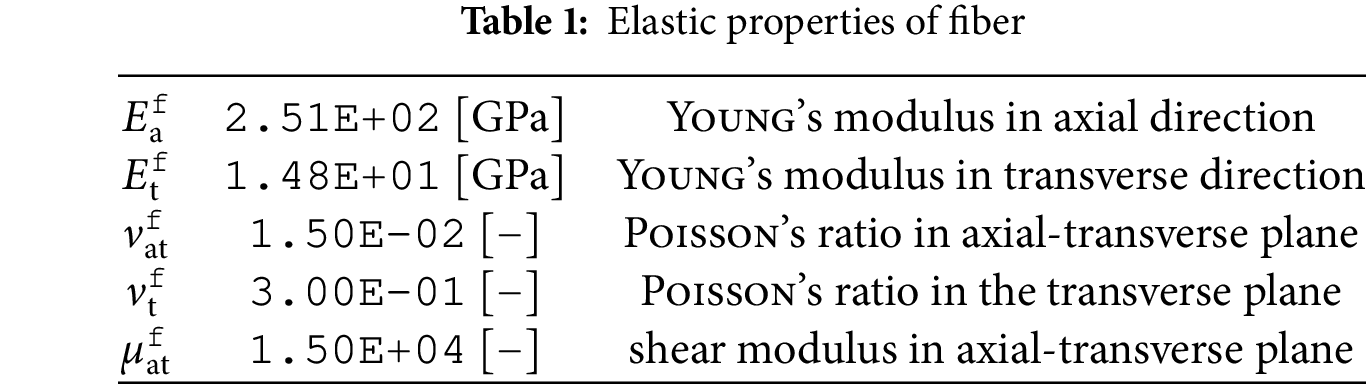
The mechanical fiber properties are given in Table 1. In this section, the yielding and ultimate strength of the matrix phase is
4.1 Verification under Transverse Uniaxial Tension Loading
Fig. 5 exhibits that the global response of 1 + 2-partition ROH under transverse uniaxial tension matches well with DNS and perfect plastic yielding can also be reproduced accurately. Figs. 6 and 7 indicate that the matrix phase starts yielding at the inner partition while the outer matrix partition remains elastic; after the outer matrix partition starts yielding, the equivalent plastic strain of the matrix only increases with
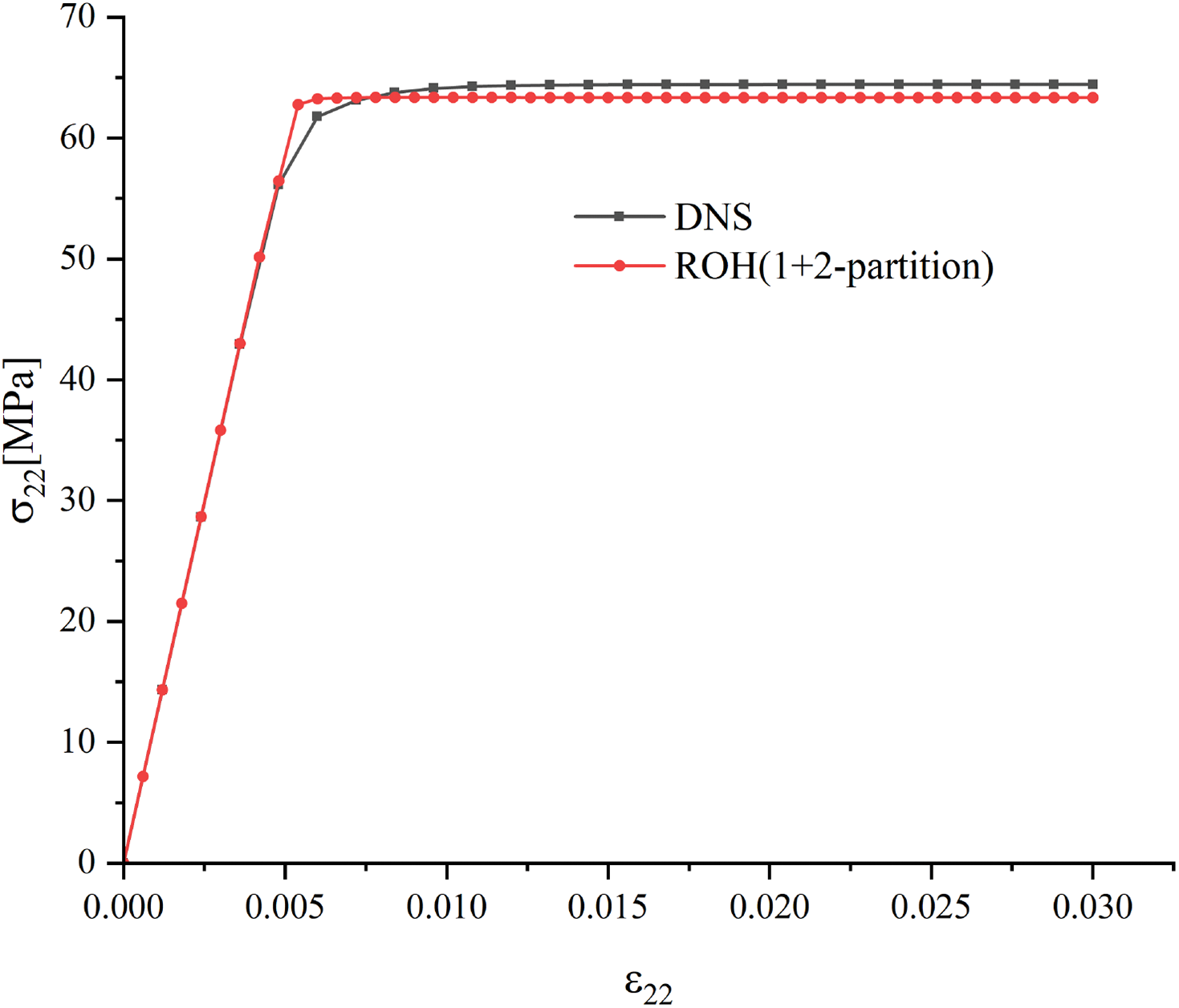
Figure 5: Stress
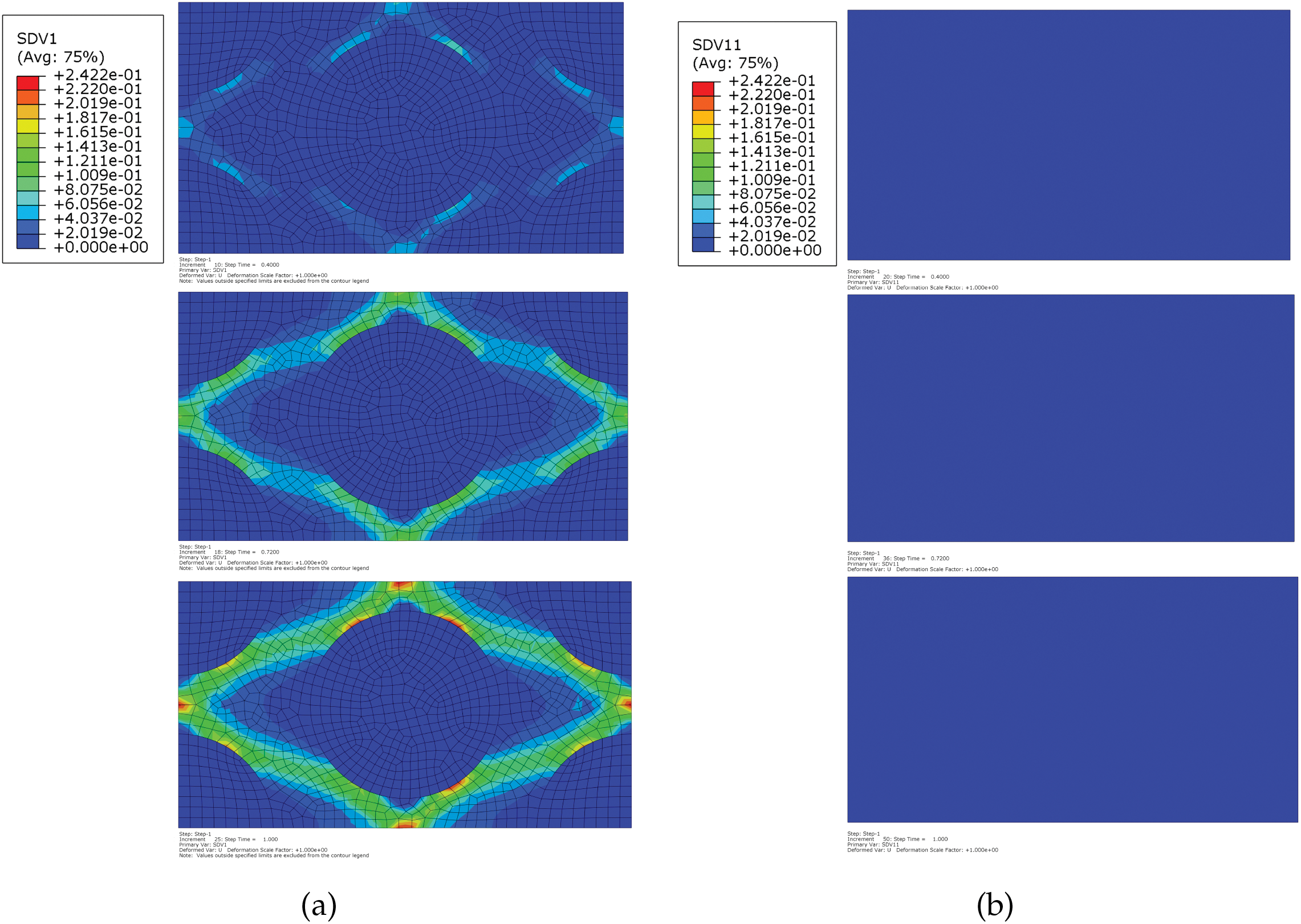
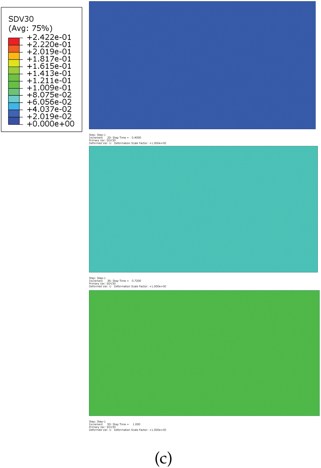
Figure 6: Comparison of the evolution of equivalent plastic strain in matrix phase under transverse uniaxial tension when the loading is
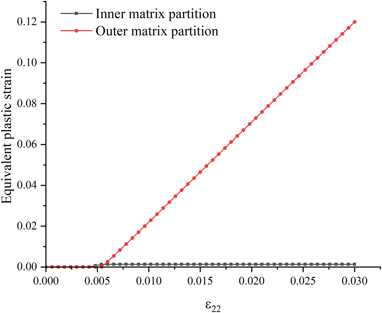
Figure 7: Evolution of equivalent plastic strains at inner and outer matrix partitions under transverse uniaxial tension:
The results of the ultimate strength of the fibrous unitcell under transverse uniaxial tension obtained through DNS, 1 + 2-partition ROH, and 1 + 1-partition ROH are presented in Figs. 8–10. The 1 + 2-partitioning scheme exhibits accuracy superiority compared to the 1 + 1-partition scheme in almost all calculation examples, especially for the cases with high fiber volume fractions. The relative errors of the 1 + 2-partition ROH method are all less than 7.3% and less than 5% in most calculation examples. On the other hand, the strength of the 1 + 1-partition ROH method always tends to be overestimated, which is a typical deficiency of the “1-phase-1-partition” method. The accuracy of 1 + 1-partition ROH is only satisfactory when
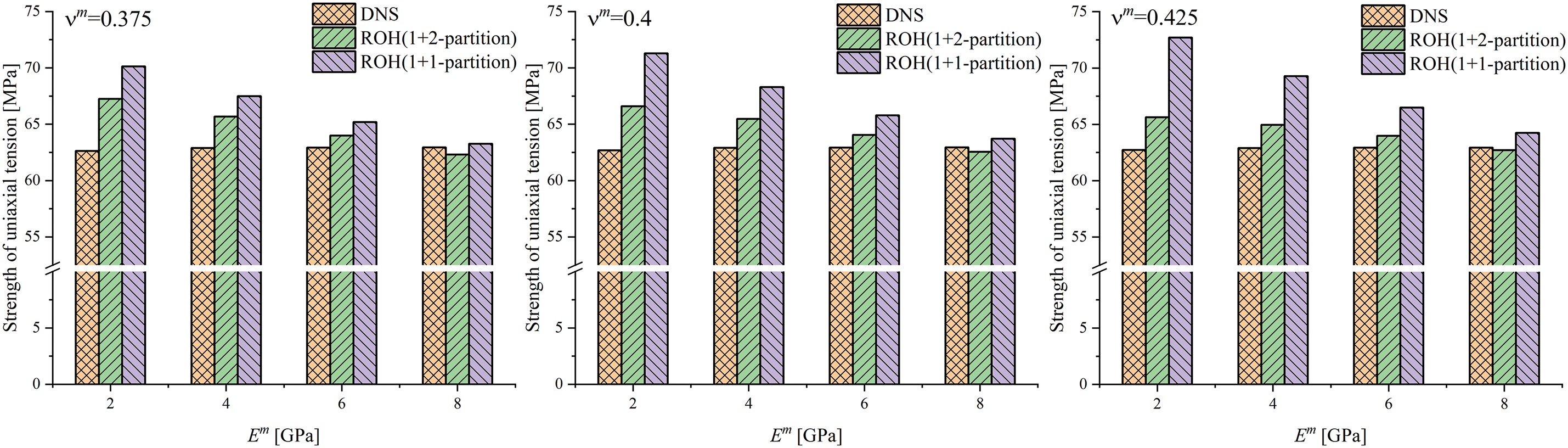
Figure 8: The comparison of ultimate strength of fibrous unitcell under transverse uniaxial tension:
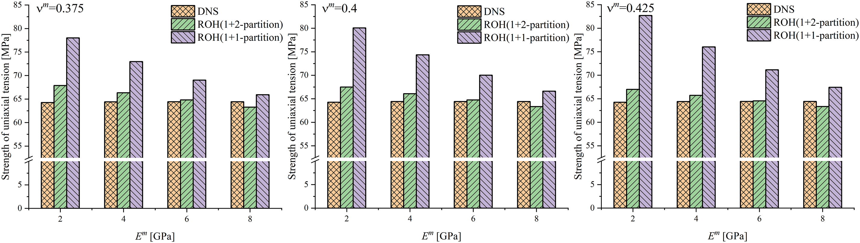
Figure 9: The comparison of ultimate strength of fibrous unitcell under transverse uniaxial tension:
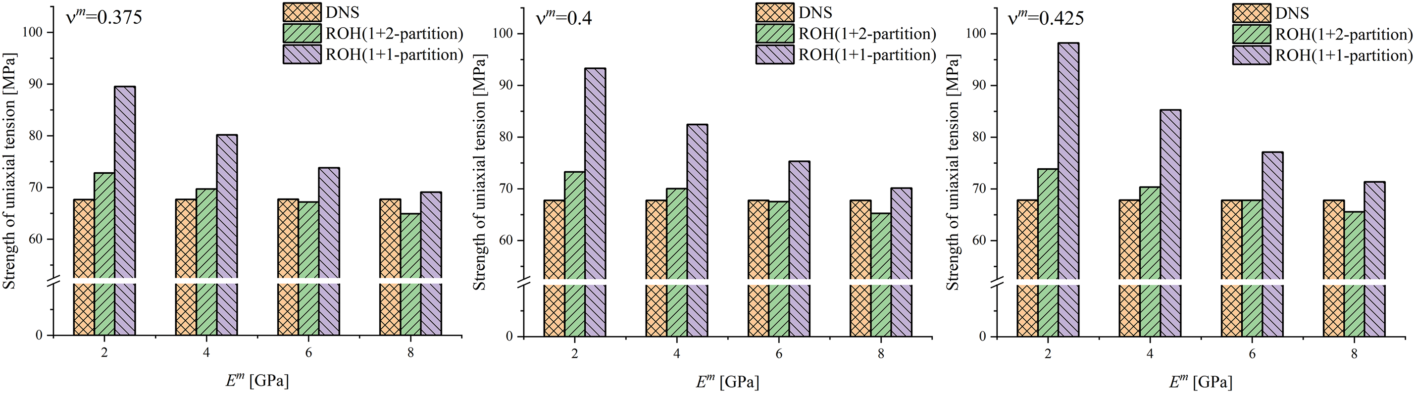
Figure 10: The comparison of ultimate strength of fibrous unitcell under transverse uniaxial tension:
4.2 Verification under Transverse Shear Loading
Fig. 11 presents the global responses of DNS and 1 + 2-partition ROH under transverse shear. The corresponding evolutions of equivalent plastic strain are given in Figs. 12 and 13. The matrix starts yielding at the interface, and then the yield area expands and grows together. Similarly, the equivalent plastic strain of the inner partition stops increasing soon after the outer partition starts yielding.
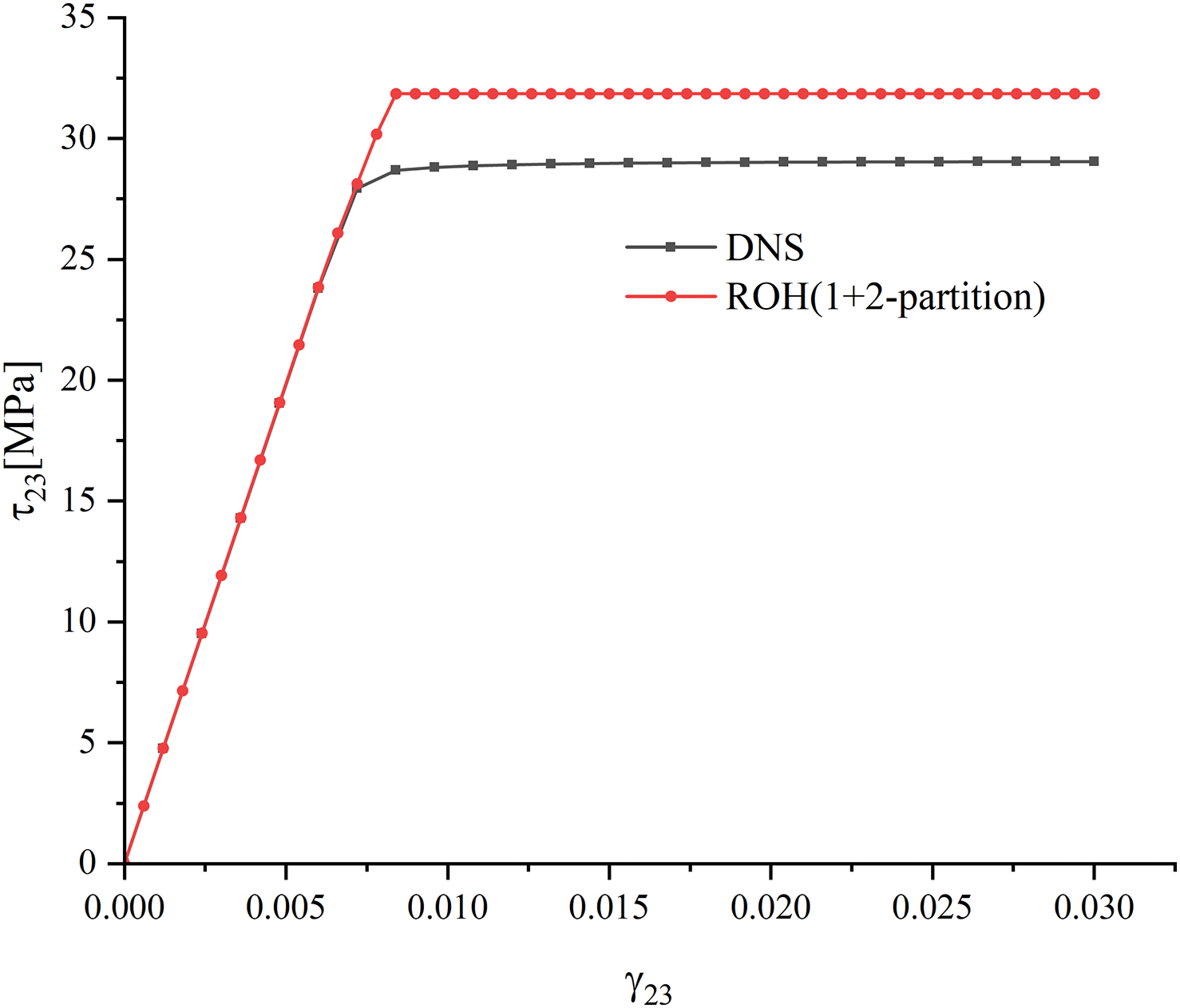
Figure 11: Stress

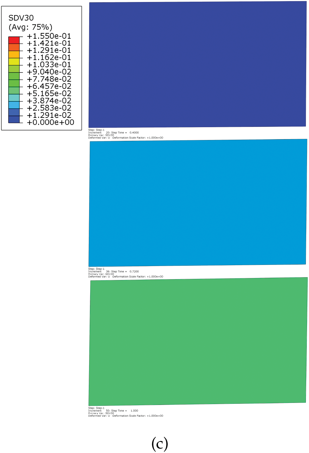
Figure 12: Comparison of the evolution of equivalent plastic strain in matrix phase under transverse shear when the loading is
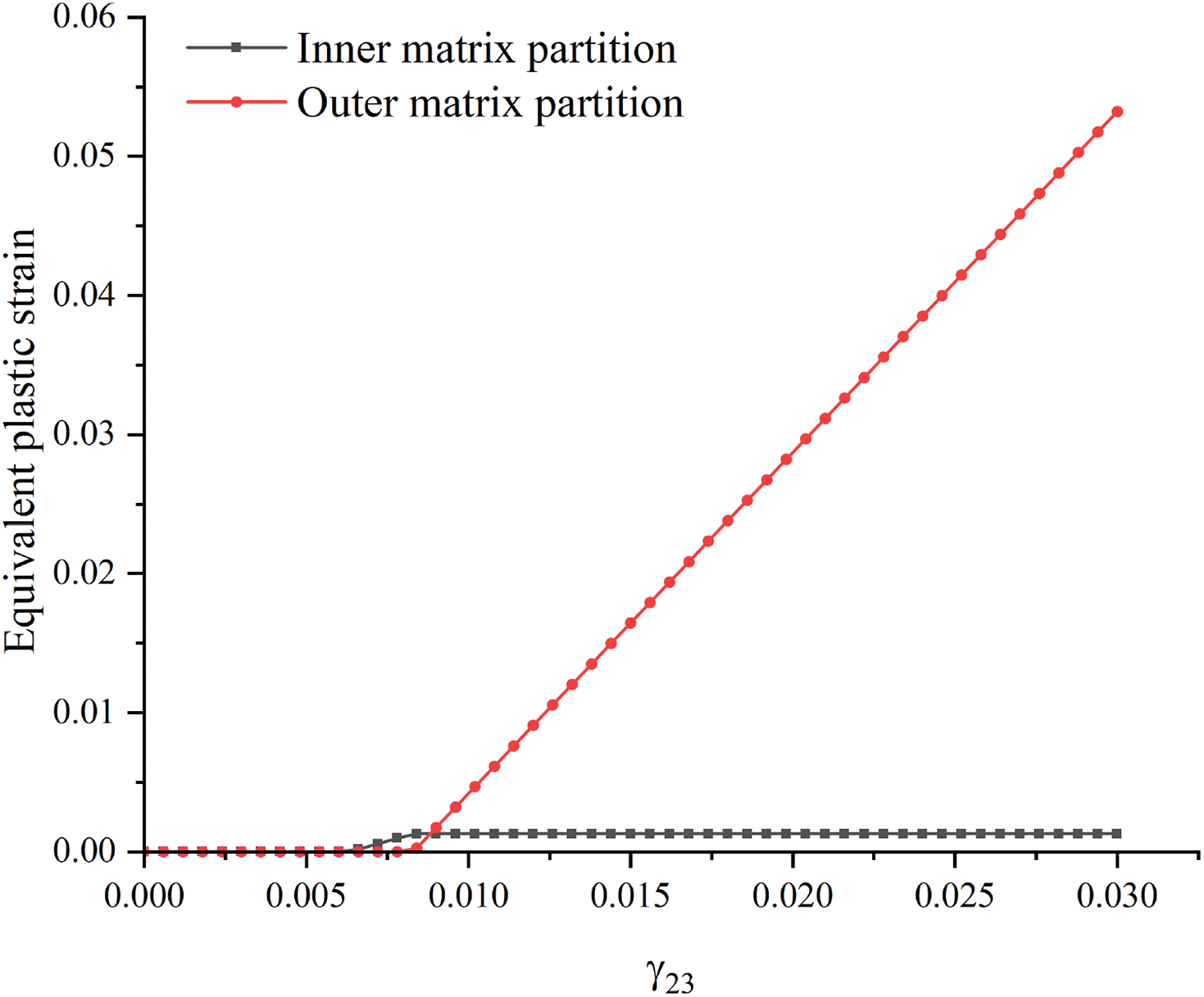
Figure 13: Evolution of equivalent plastic strains at inner and outer matrix partitions under transverse shear:
The results of ultimate strength are presented in Figs. 14–16. In the transverse shear loading problem, 1 + 2-partition ROH still presents an overall advantage over 1 + 1-partition ROH on calculation accuracy. However, the relative errors are larger than transverse uniaxial tension cases. The largest error is about 20%; in most cases, the error varies within the range of 10%–20%. On the other hand, the accuracy of 1 + 1-partition ROH is unsatisfactory in most cases. Similarly, the strengths of 1 + 1-partition ROH are all overestimated.
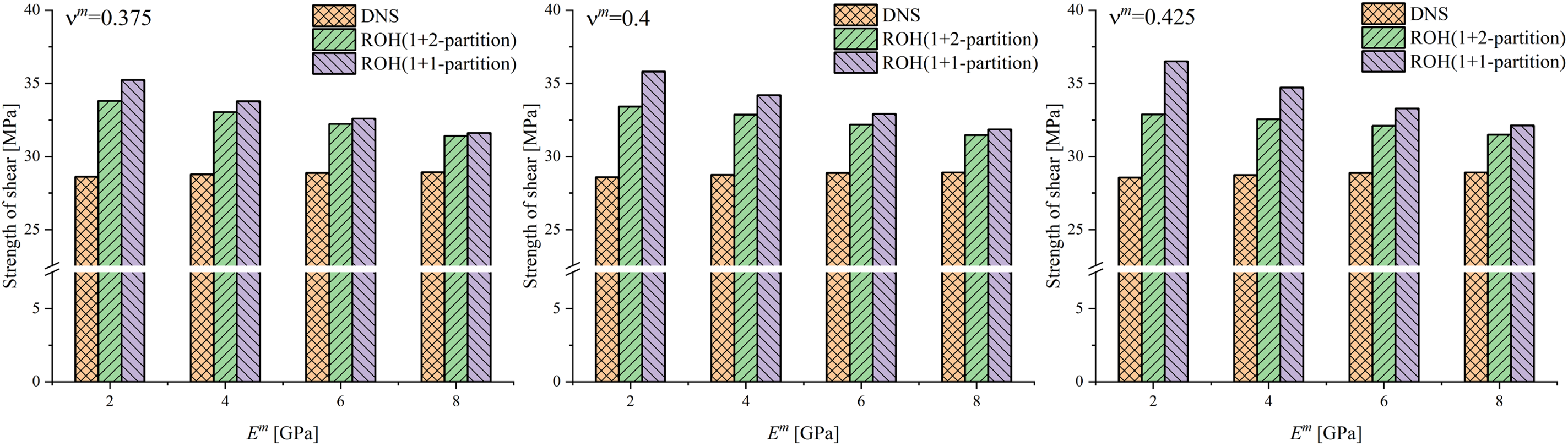
Figure 14: The comparison of ultimate strength of fibrous unitcell under transverse shear:
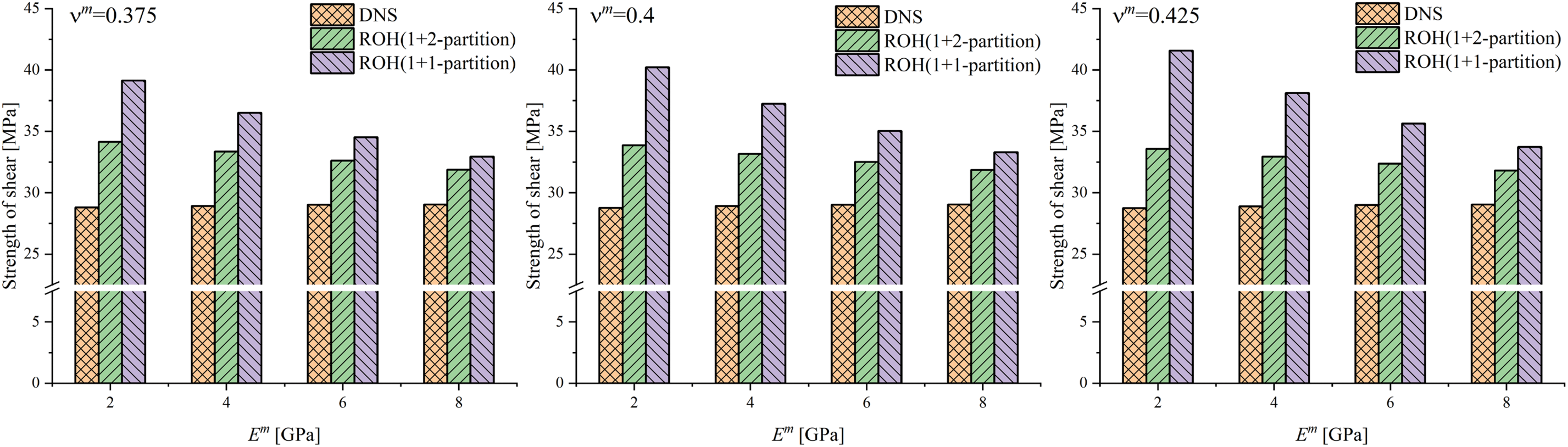
Figure 15: The comparison of ultimate strength of fibrous unitcell under transverse shear:
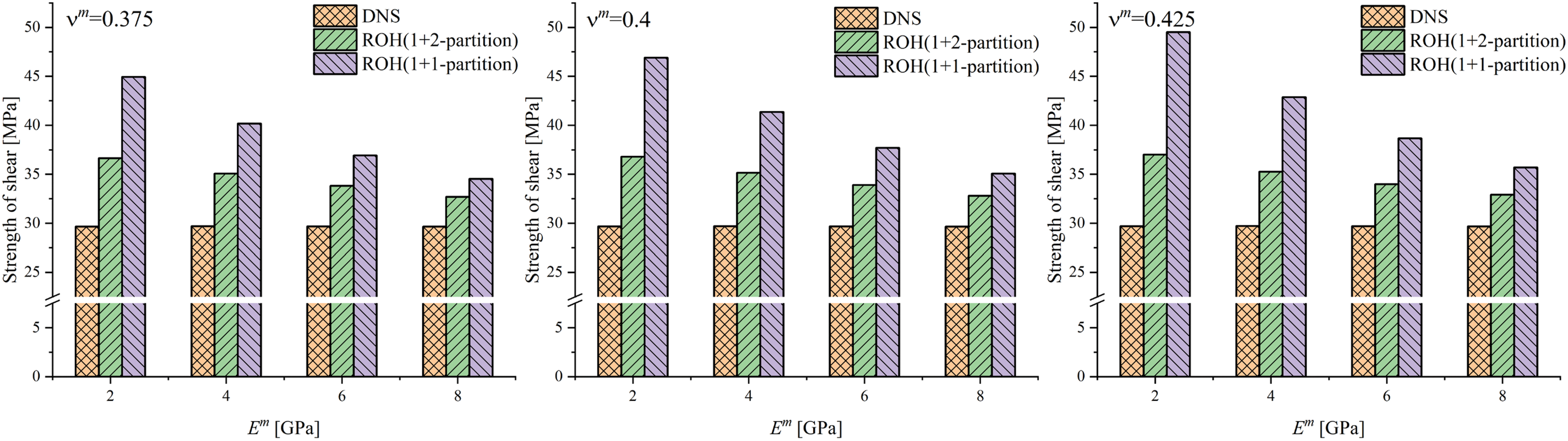
Figure 16: The comparison of ultimate strength of fibrous unitcell under transverse shear:
In this study, the 1 + 2-partitioning scheme ROH method shares the same constitutive models of fiber and matrix with the 1 + 1-partition ROH method and DNS. At the expense of an acceptable increase in the internal variables of the overall constitutive model and computation cost, the accuracy of the transverse loading problems of fibrous unitcells improves significantly compared to the typical 1 + 1-partition ROH method [44,47]. In most cases, the relative errors of the 1 + 2 partitioning method are less than 5% under transverse uniaxial tension and less than 20% under transverse shear loading, demonstrating overall improvement in accuracy compared to the 1 + 1-partition ROH method. Compared to DNS, the computation time of the 1 + 2-partition ROH method is still three orders of magnitude lower. More internal variables or partitions for the ROH method lead to higher fidelity. The 1 + 2-partition ROH method can exhibit more information on the nonlinear evolution process in a single element, as presented in Figs. 6 and 12. The benefit of the switch from 1 + 1-partition to 1 + 2-partition is considerable.
In the ROH method, the number of influence functions to be solved is
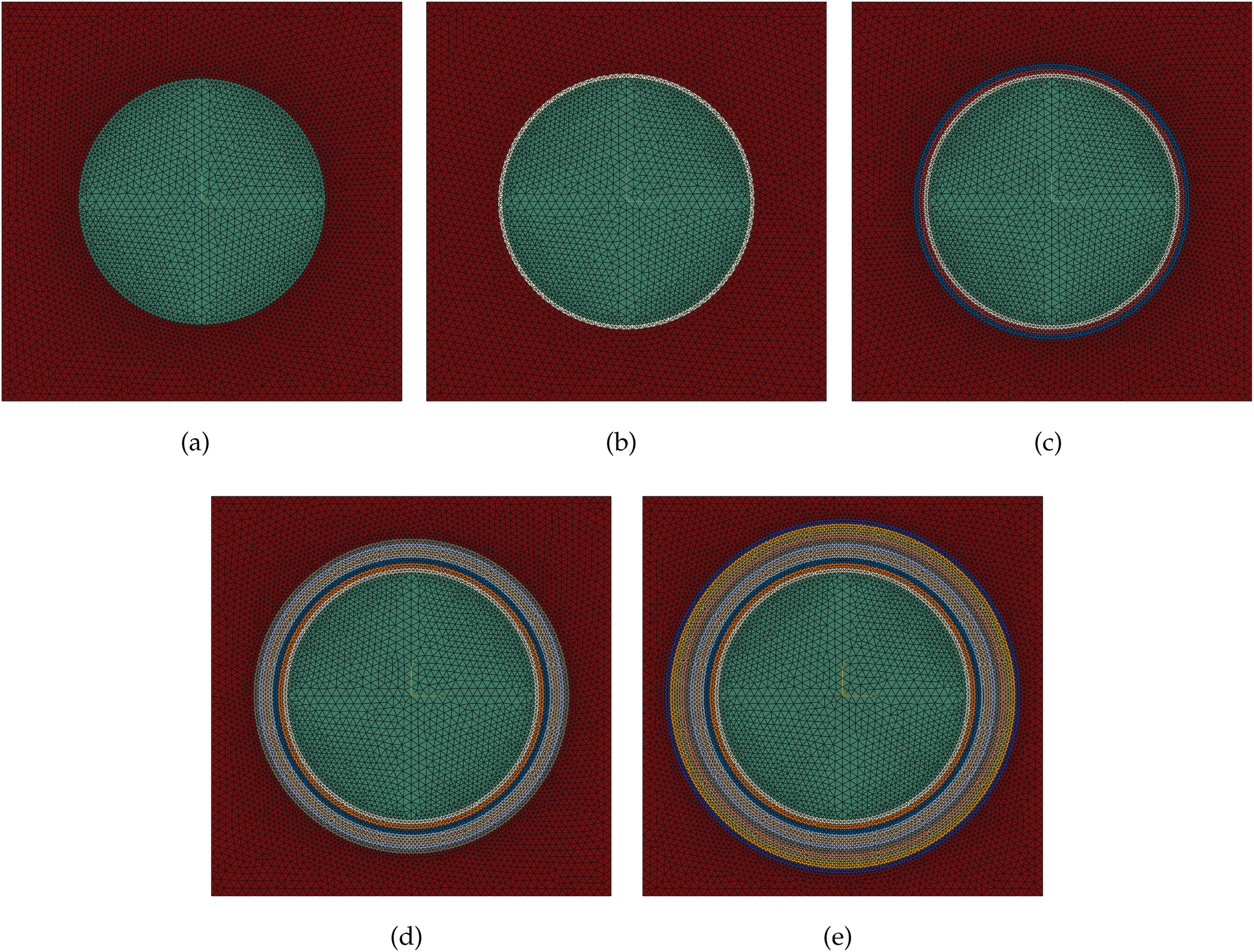
Figure 17: A sketch of fibrous unitcell finite element models with different partitionings (
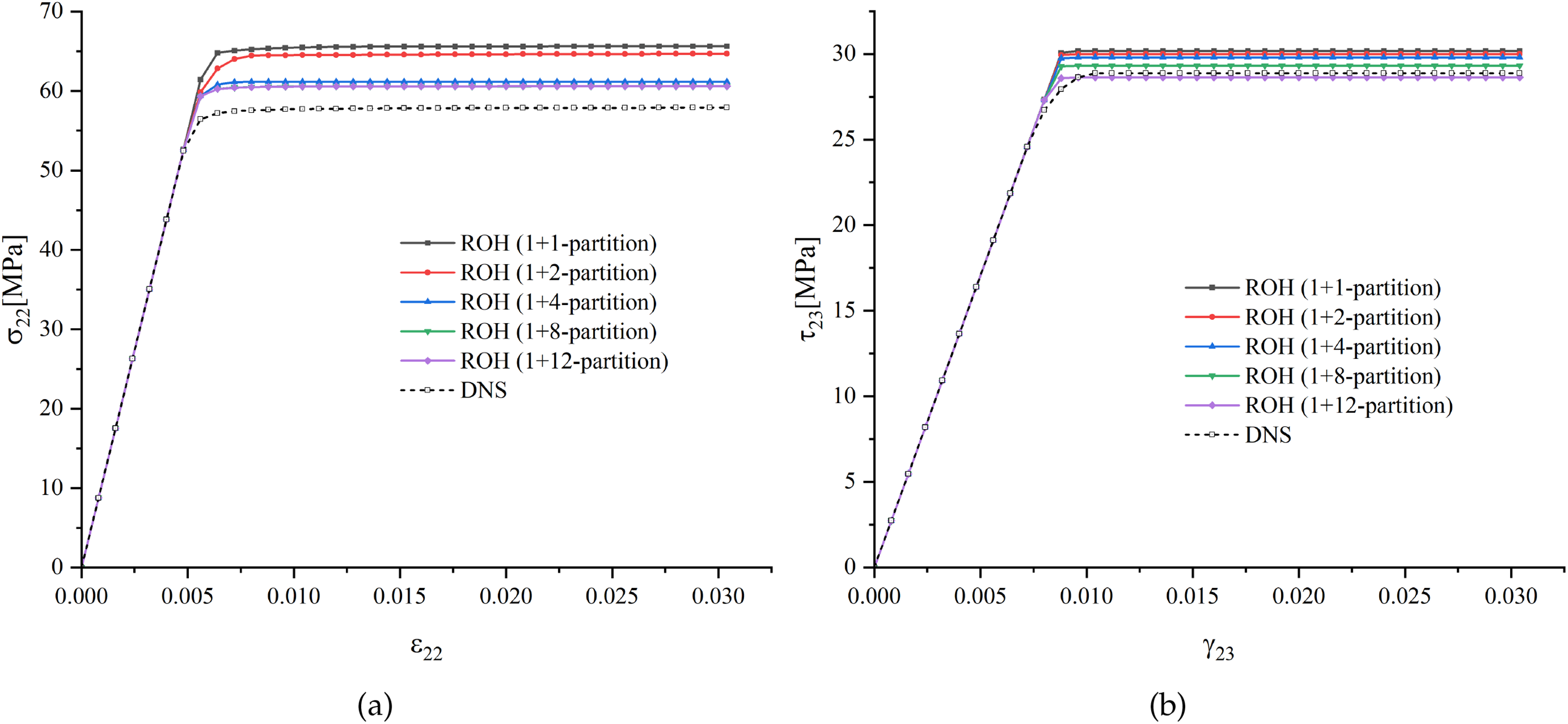
Figure 18: Global responses of fibrous unitcell under transverse loadings of different partitionings with
In addition, the influence of partitioning on computational time should also be considered. A beam model with 1000 elements is established and presented in Fig. 19, whose ROH constitutive models are obtained from the unitcells in Fig. 17 to make the impact of the number of partitions more apparent. When the beam is under uniaxial tension along the
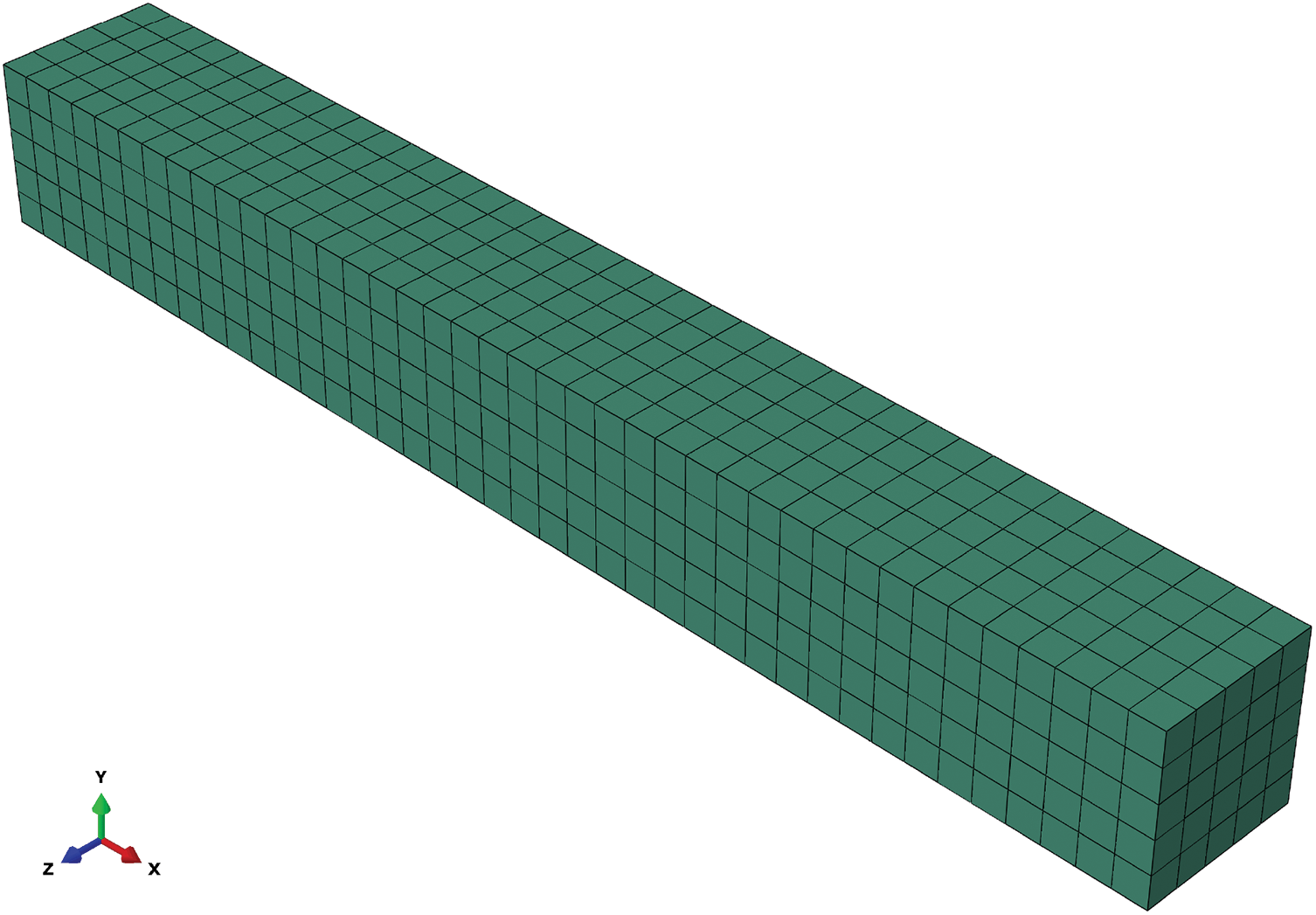
Figure 19: Beam model with multiple elements
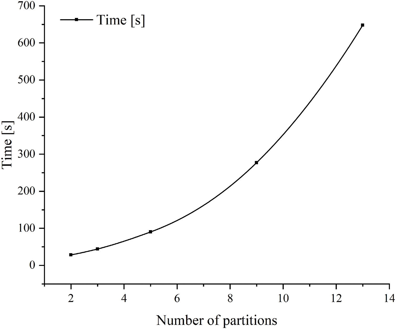
Figure 20: The variation of computation time as the number of partitions increases
The numerical method for determining the inner matrix partition volume fraction is based on a modified Eshelby method for the finite matrix domain. The
This study proposes a new overall constitutive model of the fibrous composite material to provide better accuracy for the simulation of the nonlinear responses. The matrix phase is partitioned into inner and outer partitions to capture the stress concentration within the domain of the matrix phase under transverse loadings, whose optimum volume fraction is decided by a numerical method for minimizing the error of strain energy density compared to an Eshelby method based on finite matrix domain assumption. The nonlinear evolution of the inner and outer matrix partitions are also separated so that the failure mechanism on the mesoscale is exhibited more clearly. In this model, the influence functions of three partitions are calculated by a newly proposed analytical method, which significantly reduces the computation cost of the so-called offline stage compared to the classic numerical method. For example, a rate-independent plasticity model is employed to describe the nonlinear process of the matrix phase, and a series of calculations are conducted to verify the accuracy of the proposed model when simulating the problems under transverse loadings. The accuracy of the results calculated by the new model is satisfactory and superior to that of the 1 + 1-partition ROH method within the value range in the typical application scenario of fibrous composite materials, while the increase of computation cost is limited. As the modified Eshelby method for quantifying the error of strain energy density is limited to transverse load cases, longitudinal shear loading is not involved in the optimization of inner partition volume fractions. This is the primary limitation of the present model and an area to be addressed in future improvement.
Acknowledgement: Financial support by the National Key R&D Program of China and the National Natural Science Foundation of China is gratefully acknowledged. The research is also supported by “The Fundamental Research Funds for the Central Universities, Peking University”.
Funding Statement: This work is funded by the National Key R&D Program of China (Grant No. 2023YFA1008901), the National Natural Science Foundation of China (Grant Nos. 11988102, 12172009) and “The Fundamental Research Funds for the Central Universities, Peking University”.
Author Contributions: Shanqiao Huang and Zifeng Yuan contributed to the study conceptualization, methodology, data analysis, writing, reviewing and editing. Data collection was performed by Shanqiao Huang. All authors reviewed the results and approved the final version of the manuscript.
Availability of Data and Materials: The data generated through the numerical examples included in this study are available from the corresponding author on request.
Ethics Approval: Not applicable.
Conflicts of Interest: The authors declare no conflicts of interest to report regarding the present study.
Appendix A Proof of the Semi-Positive-Definite Property of
This section studies
and prove that
Through the classic linear homogenization process based on asymptotic expansion and perturbation method, the linear homogenized elastic stiffness tensor is given as follows:
where
With Voigt notation, (A2) can be rewritten into
By Cauchy-Schwarz inequality, for arbitrary second-order tensor
Then
Repeating the same process for the matrix phase yields
Appendix B Solution of
As the first row and column of
As the first row and column of
where
As
Then the solutions of
The solutions of
Considering the distribution of non-zeros components in
After substituting (A16) and (A17) into (A14) and substituting obtained
Appendix C Solution of the Axisymmetric Elastic Problem with Bi-Material
Consider that the fiber phase and the inner partition of the matrix phase remain elastic while the second partition loses stiffness. In this case, the fibrous unitcell only has stiffness in the longitudinal direction. This section derives the displacement and strains at the fiber phase and the inner partition of the matrix phase under macroscopic strain
Due to the axisymmetric of the geometry and boundary condition, it only must solve the displacement along the radius direction
with continuity condition for the displacement
The radii
with the area of the transverse cross-section of the unitcell is
A piecewise function of
with
Accordingly, within the fiber phase, the normal strain along the radius direction gives
and for the matrix phase,
The averaged normal strain along the radius direction for the inner partition of the matrix phase gives
Appendix D Expression of Eshelby Tensors for Cylindrical Inclusion within Finite Matrix Domain
Based on the work by Ma et al. [48], the expressions of non-zero components of Eshelby tensors for a cylindrical inclusion in a finite elastic matrix are given in the following part. In these expressions,
References
1. Fish J, Wagner GJ, Keten S. Mesoscopic and multiscale modelling in materials. Nat Mat. 2021;20(6):774–86. doi:10.1038/s41563-020-00913-0. [Google Scholar] [PubMed] [CrossRef]
2. Guo Z, Hou Z, Tian X, Zhu W, Wang C, Luo M, et al. 3D printing of curvilinear fiber reinforced variable stiffness composite structures: a review. Compos Part B: Eng. 2025;291(1):112039. doi:10.1016/j.compositesb.2024.112039. [Google Scholar] [CrossRef]
3. Li Z, Wang B, Hao P, Du K, Mao Z, Li T. Multi-scale numerical calculations for the interphase mechanical properties of carbon fiber reinforced thermoplastic composites. Compos Sci Technol. 2025;260:110982. doi:10.1016/j.compscitech.2024.110982. [Google Scholar] [CrossRef]
4. Hashin Z. Failure criteria for unidirectional fiber composites. J Appl Mech. 1980 Jun;47(2):329–34. doi:10.1115/1.3153664. [Google Scholar] [CrossRef]
5. Chow CL, Wang J. An anisotropic theory of elasticity for continuum damage mechanics. Int J Fract. 1987;33(1):3–16. doi:10.1007/BF00034895. [Google Scholar] [CrossRef]
6. Camanho P, Bessa M, Catalanotti G, Vogler M, Rolfes R. Modeling the inelastic deformation and fracture of polymer composites-Part II: smeared crack model. Mech Mat. 2013;59:36–49. doi:10.1016/j.mechmat.2012.12.001. [Google Scholar] [CrossRef]
7. Canal LP, Segurado J, Llorca J. Failure surface of epoxy-modified fiber-reinforced composites under transverse tension and out-of-plane shear. Int J Sol Struct. 2009;46(11):2265–74. doi:10.1016/j.ijsolstr.2009.01.014. [Google Scholar] [CrossRef]
8. Ha SK, Jin KK, Huang Y. Micro-mechanics of Failure (MMF) for continuous fiber reinforced composites. J Compos Mat. 2008;42(18):1873–95. doi:10.1177/0021998308093911. [Google Scholar] [CrossRef]
9. Lomov SV, Ivanov DS, Verpoest I, Zako M, Kurashiki T, Nakai H, et al. Meso-FE modelling of textile composites: road map, data flow and algorithms. Compos Sci Technol. 2007;67(9):1870–91. doi:10.1016/j.compscitech.2006.10.017. [Google Scholar] [CrossRef]
10. Zhi J, Poh LH, Tay TE, Tan VBC. Direct FE2 modeling of heterogeneous materials with a micromorphic computational homogenization framework. Comput Methods Appl Mech Eng. 2022;393(1):114837. doi:10.1016/j.cma.2022.114837. [Google Scholar] [CrossRef]
11. Yuan Z, Fish J. Toward realization of computational homogenization in practice. Int J Num Meth Eng. 2008;73(3):361–80. doi:10.1002/nme.2074. [Google Scholar] [CrossRef]
12. Kouznetsova V, Geers MG, Brekelmans WM. Multi-scale constitutive modelling of heterogeneous materials with a gradient-enhanced computational homogenization scheme. Int J Num Meth Eng. 2002;54(8):1235–60. doi:10.1002/nme.541. [Google Scholar] [CrossRef]
13. Dvorak GJ. Transformation field analysis of inelastic composite materials. Proc Royal Soc London Ser A: Mathem Phys Sci. 1992;437(1900):311–27. [Google Scholar]
14. Dvorak GJ, Benveniste Y. On transformation strains and uniform fields in multiphase elastic media. Proc Royal Soc London Ser A: Mathem Phys Sci. 1992;437(1900):291–310. [Google Scholar]
15. Ng ET, Suleman A. Implicit stress integration in elastoplasticity of n-phase fiber-reinforced composites. Mech Adv Mat Struct. 2007;14(8):633–41. doi:10.1080/15376490701672302. [Google Scholar] [CrossRef]
16. Khattab IA, Sinapius M. Multiscale modelling and simulation of polymer nanocomposites using transformation field analysis (TFA). Compos Struct. 2019;209:981–91. doi:10.1016/j.compstruct.2018.10.100. [Google Scholar] [CrossRef]
17. Castrogiovanni A, Marfia S, Auricchio F, Sacco E. TFA and HS based homogenization techniques for nonlinear composites. Int J Solids Struct. 2021;225(3):111050. doi:10.1016/j.ijsolstr.2021.111050. [Google Scholar] [CrossRef]
18. Kanouté P, Boso D, Chaboche JL, Schrefler B. Multiscale methods for composites: a review. Arch Computat Meth Eng. 2009;16(1):31–75. doi:10.1007/s11831-008-9028-8. [Google Scholar] [CrossRef]
19. Wang Y, Huang Z. Analytical micromechanics models for elastoplastic behavior of long fibrous composites: a critical review and comparative study. Materials. 2018;11(10):1919. doi:10.3390/ma11101919. [Google Scholar] [PubMed] [CrossRef]
20. Spilker K, Nguyen VD, Adam L, Wu L, Noels L. Piecewise-uniform homogenization of heterogeneous composites using a spatial decomposition based on inelastic micromechanics. Compos Struct. 2022;295(3):115836. doi:10.1016/j.compstruct.2022.115836. [Google Scholar] [CrossRef]
21. Michel JC, Suquet P. Computational analysis of nonlinear composite structures using the nonuniform transformation field analysis. Comput Methods Appl Mech Eng. 2004;193(48–51):5477–502. doi:10.1016/j.cma.2003.12.071. [Google Scholar] [CrossRef]
22. Ju X, Mahnken R, Xu Y, Liang L. NTFA-enabled goal-oriented adaptive space-time finite elements for micro-heterogeneous elastoplasticity problems. Comput Methods Appl Mech Eng. 2022;398(11):115199. doi:10.1016/j.cma.2022.115199. [Google Scholar] [CrossRef]
23. Liu Z, Bessa M, Liu WK. Self-consistent clustering analysis: an efficient multi-scale scheme for inelastic heterogeneous materials. Comput Meth Appl Mech Eng. 2016;306(1):319–41. doi:10.1016/j.cma.2016.04.004. [Google Scholar] [CrossRef]
24. Kafka OL, Yu C, Shakoor M, Liu Z, Wagner GJ, Liu WK. Data-driven mechanistic modeling of influence of microstructure on high-cycle fatigue life of nickel titanium. JOM. 2018;70(7):1154–8. doi:10.1007/s11837-018-2868-2. [Google Scholar] [CrossRef]
25. Liu Z, Fleming M, Liu WK. Microstructural material database for self-consistent clustering analysis of elastoplastic strain softening materials. Comput Meth Appl Mech Eng. 2018;330(41):547–77. doi:10.1016/j.cma.2017.11.005. [Google Scholar] [CrossRef]
26. Liu Z, Kafka OL, Yu C, Liu WK. Data-driven self-consistent clustering analysis of heterogeneous materials with crystal plasticity. In: Computational methods in applied sciences. Cham: Springer International Publishing; 2018. Vol. 46, p. 221–42. [Google Scholar]
27. Yu C, Kafka OL, Liu WK. Self-consistent clustering analysis for multiscale modeling at finite strains. Comput Meth Appl Mech Eng. 2019;349(5330):339–59. doi:10.1016/j.cma.2019.02.027. [Google Scholar] [CrossRef]
28. Zhang L, Tang S. Displacement reconstruction and strain refinement of clustering-based homogenization. Theor Appl Mech Lett. 2021;11(6):100285. doi:10.1016/j.taml.2021.100285. [Google Scholar] [CrossRef]
29. Tang S, Zhu X. Clustering solver for displacement-based numerical homogenization. Theor Appl Mech Lett. 2022;12(3):100306. doi:10.1016/j.taml.2021.100306. [Google Scholar] [CrossRef]
30. Ri JH, Hong HS, Ri SG. Cluster based nonuniform transformation field analysis: an efficient homogenization for inelastic heterogeneous materials. Int J Num Meth Eng. 2021;122(17):4458–85. doi:10.1002/nme.6696. [Google Scholar] [CrossRef]
31. Ri JH, Ri UI, Hong HS. Multiscale analysis of elastic-viscoplastic composite using a cluster-based reduced-order model. Compos Struct. 2021;272:114209. doi:10.1016/j.compstruct.2021.114209. [Google Scholar] [CrossRef]
32. Tang S, Zhang L, Liu WK. From virtual clustering analysis to self-consistent clustering analysis: a mathematical study. Computat Mech. 2018;62(6):1443–60. doi:10.1007/s00466-018-1573-x. [Google Scholar] [CrossRef]
33. Cheng G, Li X, Nie Y, Li H. FEM-Cluster based reduction method for efficient numerical prediction of effective properties of heterogeneous material in nonlinear range. Comput Meth Appl Mech Eng. 2019;348:157–84. doi:10.1016/j.cma.2019.01.019. [Google Scholar] [CrossRef]
34. Bessa MA, Bostanabad R, Liu Z, Hu A, Apley DW, Brinson C, et al. A framework for data-driven analysis of materials under uncertainty: countering the curse of dimensionality. Comput Meth Appl Mech Eng. 2017;320(1):633–67. doi:10.1016/j.cma.2017.03.037. [Google Scholar] [CrossRef]
35. Han X, Xu C, Xie W, Meng S. Multiscale computational homogenization of woven composites from microscale to mesoscale using data-driven self-consistent clustering analysis. Compos Struct. 2019;220:760–8. doi:10.1016/j.compstruct.2019.03.053. [Google Scholar] [CrossRef]
36. Li H, Kafka OL, Gao J, Yu C, Nie Y, Zhang L, et al. Clustering discretization methods for generation of material performance databases in machine learning and design optimization. Comput Mech. 2019;64(2):281–305. doi:10.1007/s00466-019-01716-0. [Google Scholar] [CrossRef]
37. Zhang L, Lu Y, Tang S, Liu WK. HiDeNN-TD: reduced-order hierarchical deep learning neural networks. Comput Methods Appl Mech Eng. 2022;389(39–41):114414. doi:10.1016/j.cma.2021.114414. [Google Scholar] [CrossRef]
38. Lu Y, Li H, Saha S, Mojumder S, Al Amin A, Suarez D, et al. Reduced order machine learning finite element methods: concept, implementation, and future applications. Comput Model Eng Sci. 2021;129(3):1351–71. doi:10.32604/cmes.2021.017719. [Google Scholar] [CrossRef]
39. Fish J, Yu Y. Data-physics driven reduced order homogenization. Int J Numer Meth Eng. 2023;124(7):1620–45. doi:10.1002/nme.7178. [Google Scholar] [CrossRef]
40. Yu Y, Fish J. Data-physics driven reduced order homogenization for continuum damage mechanics at multiple scales. Int J Multiscale Computat Eng. 2024;22(1):1–14. doi:10.1615/IntJMultCompEng.2023049164. [Google Scholar] [CrossRef]
41. Lefik M, Boso DP, Schrefler BA. Artificial Neural Networks in numerical modelling of composites. Comput Methods Appl Mech Eng. 2009;198(21–26):1785–804. doi:10.1016/j.cma.2008.12.036. [Google Scholar] [CrossRef]
42. Liu Z, Wu CT, Koishi M. A deep material network for multiscale topology learning and accelerated nonlinear modeling of heterogeneous materials. Comput Meth Appl Mech Eng. 2019;345(4):1138–68. doi:10.1016/j.cma.2018.09.020. [Google Scholar] [CrossRef]
43. Masrouri M, Qin Z. Towards data-efficient mechanical design of bicontinuous composites using generative AI. Theor Appl Mech Lett. 2024;14(1):100492. doi:10.1016/j.taml.2024.100492. [Google Scholar] [CrossRef]
44. Oskay C, Fish J. Eigendeformation-based reduced order homogenization for failure analysis of heterogeneous materials. Comput Meth Appl Mech Eng. 2007;196(7):1216–43. doi:10.1016/j.cma.2006.08.015. [Google Scholar] [CrossRef]
45. Yue J, Yuan Z. A study on equivalence of nonlinear energy dissipation between first-order computational homogenization (FOCH) and reduced-order homogenization (ROH) methods. Theor Appl Mech Lett. 2021;11(1):100225. doi:10.1016/j.taml.2021.100225. [Google Scholar] [CrossRef]
46. Huang S, Yue J, Liu X, Ren P, Zu L, Yuan Z. A framework of defining constitutive model for fibrous composite material through reduced-order-homogenization method with analytical influence functions. Compos Struct. 2023;314(2):116968. doi:10.1016/j.compstruct.2023.116968. [Google Scholar] [CrossRef]
47. Fish J, Filonova V, Yuan Z. Hybrid impotent-incompatible eigenstrain based homogenization. Int J Num Meth Eng. 2013;95(1):1–32. doi:10.1002/nme.4473. [Google Scholar] [CrossRef]
48. Ma H, Gao XL. Strain gradient solution for a finite-domain Eshelby-type plane strain inclusion problem and Eshelby’s tensor for a cylindrical inclusion in a finite elastic matrix. Int J Sol Struct. 2011;48(1):44–55. doi:10.1016/j.ijsolstr.2010.09.004. [Google Scholar] [CrossRef]
49. Li S, Wang G, Sauer RA. The eshelby tensors in a finite spherical domain—part II: applications to homogenization. J Appl Mech, Transact ASME. 2007;74(4):784–97. doi:10.1115/1.2711228. [Google Scholar] [CrossRef]
50. Li S, Sauer RA, Wang G. The eshelby tensors in a finite spherical domain—part I: theoretical formulations. J Appl Mech. 2007;74(4):770–83. doi:10.1115/1.2711227. [Google Scholar] [CrossRef]
51. Li S, Wang G. Introduction to micromechanics and nanomechanics. 2nd ed. Singapore: World Scientific; 2017. [Google Scholar]
52. Fish J. Practical multiscaling. Hoboken, NJ, USA: John Wiley & Sons; 2013. [Google Scholar]
Cite This Article
 Copyright © 2025 The Author(s). Published by Tech Science Press.
This work is licensed under a Creative Commons Attribution 4.0 International License , which permits unrestricted use, distribution, and reproduction in any medium, provided the original work is properly cited.
 Downloads
 Citation Tools