Optical Solitons with Parabolic and Weakly Nonlocal Law of Self-Phase Modulation by Laplace–Adomian Decomposition Method

1  Introduction

Over six decades ago, N. J. Zabusky and M. D. Kruskal introduced the concept of a soliton to describe a stable solitary wave propagating through a nonlinear medium [1]. However, they were not the first to recognize the remarkable properties of solitary waves; this notion can be traced back to the 18th-century observations of John Scott Russell, who described such waves as “a massive solitary elevation, a rounded, smooth, and well-defined mound of water” in a canal near Edinburgh. A. Hasegawa and F. Tappert made significant contributions to the field in 1973 by writing two important papers on nonlinear pulse transmission. These papers set the stage for the study of optical solitons and nonlinear fiber optics [2,3]. Since the publication of Hasegawa and Tappert’s work, the theoretical and experimental inquiry into solitary waves has proliferated across multiple scientific disciplines, encompassing applied mathematics, physics, chemistry, and biology. We mainly classify solitons into two types: bright solitons and dark solitons. The bright ones appear as localized peaks or pulses of intensity above a zero or low background, while the dark ones appear as localized dips or holes in the intensity of a continuous wave background.

A wide variety of significant equations, in both canonical and extended formats, have arisen as universal models for describing soliton propagation. The Nonlinear Schrödinger Equation (NLSE) serves as the principal model for describing soliton propagation dynamics in optical fibers. Various models elucidate soliton dynamics depending on distinct physical conditions. Among the several mathematical models employed to characterize soliton dynamics, there exists a relatively novel NLSE in the literature that demonstrates a unique form of nonlinearity, despite its recent observations. This NLSE, which is the primary focus of our article, results from the connection between the nonlinearity of a nonlocal medium and parabolic law nonlinearity [4].

Optical solitons are unique light pulses that retain their shape and velocity as they traverse a medium, even over extended distances. This distinctive characteristic is the result of a delicate equilibrium between two effects: dispersion and nonlinearity. The actual importance of optical solitons can be observed in their numerous applications, particularly in [5]:

Long-distance optical communication: Solitons facilitate the transmission of high-speed data over extensive distances with minimal signal degradation. This is essential for the operation of transoceanic and continental communication networks.

High-capacity optical networks: Solitons offer a greater bandwidth and higher data rates in optical communication systems by maintaining pulse integrity.

On the other hand, in the mid-1980s, G. Adomian and R. Rach merged the Adomian method with the renowned Laplace transform [6,7], resulting in what is currently referred to as the Laplace-Adomian decomposition method (LADM). The LADM technique can be implemented without linearizing the problem being solved. This method provides a solution represented as a convergent series with readily calculable components; often, the series converges rapidly, requiring just a limited number of terms to understand the behavior of the solutions. One of the compelling features in the study of optical solitons is the ability to address them numerically. This is in addition to the analytical results that has flooded the journals. There are several analytical approaches that have been successfully implemented to recover these soliton solutions analytically. Incidentally, numerical simulations are also visible across several papers. However, the results from numerics are very few and far between. The Adomian decomposition, the variational iteration approach, the enhanced Adomian decomposition scheme, and the Laplace-Adomian decomposition method (LADM) are some of the numerical algorithms that have been utilized [8].

The current paper will be address in the nonlinear Schrödinger’s equation by this LADM scheme that would furnish results that are visually captivating. Both bright and dark soliton solutions would be addressed. The LADM scheme would first yield the Adomian polynomials, and the scheme would display a few surface plots of such solitons. In addition, the density plots of the solitons are shown. Finally, the error plots are exhibited along with the tables for the error measure. This error is remarkably small with regard to bright and dark soliton solutions. The paper first introduces the model, and the known analytical results are recapitulated. This is followed by the corresponding Adomian polynomials, and the transparent numerical results are finally there. Details continue in the subsequent section.

2  Solitons and Dynamic Model Formulation Equation

The propagation dynamics of soliton molecules in an optical fiber, characterized by parabolic law nonlinearity and also a weakly nonlocal nonlinearity component, are articulated by the dimensionless form of the model equation, expressed as [9,10]:

iqt+aqxx+(b1|q|2|+b2|q|4|)q+b3(|q|2)xxq=0.(1)

In this equation, the first component on the left side represents the evolution over time, the group-velocity dispersion (GVD) is represented by a, and the complex imaginary unit is written as i. The coefficients of b1 and b2, which are taken from cubic and quintic nonlinear forms, respectively, and constitute the two nonlinear parameters. The binding of these two components causes these two actions to have a cumulative nonlinear effects. The coefficient of b3, which is a result of weak non-local nonlinearity, is accounted for by the third nonlinear effect [11–13]. In [13], the authors used various versions of the solitary wave ansatz to identify a wide variety of solitons for Eq. (1). Some of the most recent and important works that address the study of highly dispersive solitons for the NLSE through Ansatz are [14–16] and [17].

2.1 Bright Solitons

The bright soliton solution to (1) has just been found by the authors in [13] using ansatz techniques, which is expressed as

q(x,t)=A1(sech⁡[B1(x−νt)])ei(−κx+ωt+Θ).(2)

In Eq. (2), the wave’s speed is denoted by ν, its wave number is denoted by κ, the soliton frequency is represented by ω, and the phase center constant is denoted by Θ.

It is possible to define the amplitude A1 of the bright soliton as well as the inverse width B1 in the following manner:

A1=ab2−3b1b32b2b3,(3)

B1=ab2−3b1b312b32.(4)

We also have the following relation between the model parameters

ν=−2aκ,ω=a(B2−κ2).(5)

The following conditions must be satisfied in order for bright solitons to exist:

{b2b3>0,ab2−3b1b3>0,(6)

or,

{b2b3<0,ab2−3b1b3<0.(7)

2.2 Dark Solitons

The dark soliton solution to (1) has just been found by the authors in [13] using ansatz techniques, which is expressed as

q(x,t)=A2(tanh⁡[B2(x−νt)])ei(−κx+ωt+Θ).(8)

In Eq. (8), the wave’s speed is denoted by ν, its wave number is denoted by κ, the soliton frequency is represented by ω, and the phase center constant is denoted by Θ.

It is possible to define the amplitude A2 of the dark soliton as well as the inverse width B2 in the following manner:

A2=ab2−3b1b34b2b3,(9)

B2=3b1b3−ab224b32.(10)

We also have the following relation between the model parameters

ν=−2aκ,ω=−2aB2+2b3A2B2−aκ2.(11)

The following conditions must be satisfied in order for dark solitons to exist:

{b2b3<0,3b1b3−ab2>0,(12)

or,

{b2b3<0,ab2−3b1b3<0.(13)

3  The Laplace-Adomian Decomposition Method

This section will present an overview of the Adomian decomposition technique, which is well-known, as well as its enhancement, which is the consequence of its integration with the Laplace transform [6,18,19]. The main objective of the development process is to accomplish the evolution of both bright and dark solitons for the model that correspond to by the nonlinear Schrödinger Eq. (1).

Usually, we may express Eq. (1) using operators as

(Dt+R+N)q(x,t)=0(14)

subject to the initial condition

q(x,0)=f(x),(15)

Nq(x,t)=(b1|q|2+b2|q|4+b3(|q|2)xx)q,(16)

Nq(x,t)=b1q2q∗+b2q3q∗2+b3q2qxx∗+2b3qqxqx∗+b3qqxxq∗.(17)

An unknown function q may be split through an unlimited number of summands described by the decomposition series using the conventional Adomian decomposition approach:

q(x,t)=∑n=0∞qn(x,t),(18)

where each of the components qn(x,y) need to be calculated iteratively. The goal of the decomposition approach is to locate each component q1, q2, q3,⋯ independently, with q0 being the starting condition. The nonlinear component is further decomposed using the Adomian approach in the following way:

Nq(x,t)=∑n=0∞Qn(q0,…,qn),(19)

where Qn denotes all Adomian polynomials [20,21].

According to Eq. (17), the nonlinear operatorN may be broken down into the following components:

Nq(x,t)=(N1+N2+N3+N4+N5)q(x,t),(20)

where

N1(q)=b1q2q∗,N2(q)=b2q3q∗2,N3(q)=b3q2qxx∗,N4(q)=2b3qqxqx∗,N5(q)=b3qqxxq∗.(21)

There is a decomposition into an infinite number of Adomian polynomials that may be applied to any nonlinear term N1,…,N5. The decomposition has the following structure:

Nj(q)=∑n=0∞𝒬nj(q0,q1,…,qn),j=1,2,…,5.(22)

For each j=1,2,…,5, the Adomian polynomials are represented by Qnj in (22), and they are to be created using the equations given in [21]:

Qnj(q0,q1,…,qn)={Nj(q0),n=01n∑k=0n−1(k+1)qk+1∂∂q0Qn−k−1j,n=1,2,3,…(23)

In [22–24], the series convergence (22) is explored further.

From this point forward, we shall denote the Laplace transform as ℒ and the inverse operator as ℒ−1. The result is obtained by applying ℒ to both sides of the functional Eq. (14) results in

ℒ{Dtq(x,t)}=−ℒ{Rq(x,t)+Nq(x,t)}.(24)

When we take into account the initial condition, which will be established by the first profiles of the solitons, we get the expression f(x)=q(x,0), we obtain

ℒ{q(x,t)}=1s[q(x,0)−(ℒ{Rq(x,t)+Nq(x,t)})].(25)

By substituting Eqs. (18) and (22) into Eq. (25), the result is

ℒ{∑n=0∞qn(x,t)}=1s[q(x,0)−(ℒ{R(∑n=0∞qn(x,t))+∑j=15∑n=0∞Qnj(q0,…,qn)}].(26)

The Laplace transform of each component of the solution qm may be obtained by equating the two sides of Eq. (26), which resulted in the following:

sℒ{q0(x,t)}=q(x,0)(27)

Furthermore, the recursive relations are shown as follows for every m≥1:

sℒ{qm(x,t)}=−(ℒ{Rqm−1(x,t)}+ℒ{∑j=15∑n=0∞Qm−1j(q0,…,qn)}).(28)

In order to calculate a significant number of Adomian polynomials, we will use the q-variable nonlinear operators Nj found in Eq. (21). The following is produced by using Eq. (23):

Q01=b1q02q0∗,Q11=b1(q1∗q02+2q0∗q1q0),Q21=b1(q2∗q02+q0∗q12+2q0∗q2q0+2q1∗q1q0),Q31=b1(q3∗q02+q1∗q12+2q2∗q1q0+2q1∗q2q0+2q0∗q3q0+2q0∗q1q2),Q41=b1(q4∗q02+q2∗q12+q0∗q22+2q3∗q1q0+2q2∗q2q0+2q1∗q3q0+2q0∗q4q0+2q1∗q1q2+2q0∗q1q3),

⋮

Q02=b2q0∗2q03,Q12=b2(2q0∗q1∗q03+3q0∗2q1q02),Q22=b2(q1∗2q03+2q0∗q2∗q03+6q0∗q1∗q1q02+3q0∗2q2q02+3q0∗2q12q0),Q32=b2(2q1∗q2∗q03+2q0∗q3∗q03+3q1∗2q1q02+6q0∗q2∗q1q02+6q0∗q1∗q2q02+3q0∗2q3q02+6q0∗q1∗q12q0+6q0∗2q1q2q0+q0∗2q13),Q42=b2(q2∗2q03+2q1∗q3∗q03+2q0∗q4∗q03+6q1∗q2∗q1q02+6q0∗q3∗q1q02+3q1∗2q2q02+6q0∗q2∗q2q02+6q0∗q1∗q3q02+3q0∗2q4q02+3q1∗2q12q0+6q0∗q2∗q12q0+3q0∗2q22q0+12q0∗q1∗q1q2q0+6q0∗2q1q3q0+2q0∗q1∗q13+3q0∗2q12q2),

⋮

Q03=b3q02q0xx∗,Q13=b3(q02q1xx∗+2q0q1q0xx∗),Q23=b3(q12q0xx∗+2q0q2q0xx∗+2q0q1q1xx∗+q02q2xx∗),Q33=b3(q12q1xx∗+2q1q2q0xx∗+2q0q3q0xx∗+2q0q2q1xx∗+2q0q1q2xx∗+q02q3xx∗),Q43=b3(q12q2xx∗+2q1q2q1xx∗+q22q0xx∗+2q1q3q0xx∗+2q0q4q0xx∗+2q0q3q1xx∗+2q0q2q2xx∗+2q0q1q3xx∗+q02q4xx∗),

⋮

Q04=2b3q0q0x∗q0x,Q14=2b3(q0q0x∗q1x+q0q1x∗q0x+q1q0x∗q0x),Q24=2b3(q0q0x∗q2x+q0q1x∗q1x+q0q2x∗q0x+q1q0x∗q1x+q1q1x∗q0x+q2q0x∗q0x),Q33=2b3(q0q0x∗q3x+q0q1x∗q2x+q0q2x∗q1x+q0q3x∗q0x+q1q0x∗q2x+q1q1x∗q1x+q1q2x∗q0x+q2q0x∗q1x+q2q1x∗q0x+q3q0x∗q0x),Q44=2b3(q0q0x∗q4x+q0q1x∗q3x+q0q2x∗q2x+q0q3x∗q1x+q0q4x∗q0x+q1q0x∗q3x+q1q1x∗q2x+q1q2x∗q1x+q1q3x∗q0x+q2q0x∗q2x+q2q1x∗q1x+q2q2x∗q0x+q3q0x∗q1x+q3q1x∗q0x+q4q0x∗q0x),

⋮

Q05=b3q0∗q0q0xx,Q15=b3(q1∗q0q0xx+q0∗q1q0xx+q0∗q0q1xx),Q25=b3(q2∗q0q0xx+q1∗q1q0xx+q0∗q2q0xx+q1∗q0q1xx+q0∗q1q1xx+q0∗q0q2xx),Q35=b3(q3∗q0q0xx+q2∗q1q0xx+q1∗q2q0xx+q0∗q3q0xx+q2∗q0q1xx+q1∗q1q1xx+q0∗q2q1xx+q1∗q0q2xx+q0∗q1q2xx+q0∗q0q3xx),Q45=b3(q4∗q0q0xx+q3∗q1q0xx+q2∗q2q0xx+q1∗q3q0xx+q0∗q4q0xx+q3∗q0q1xx+q2∗q1q1xx+q1∗q2q1xx+q0∗q3q1xx+q2∗q0q2xx+q1∗q1q2xx+q0∗q2q2xx+q1∗q0q3xx+q0∗q1q3xx+q0∗q0q4xx),

for further Adomian polynomials, etc.

Lastly, the components q0, q1, q2,… are found by calculating in the inverse Laplace transform ℒ−1:

{q0(x,t)=q(x,0),q1(x,t)=−ℒ−1(1sℒ{Rq0(x,t)}+1s[ℒ{∑j=15Q0j(q0,…,qn)}]),q2(x,t)=−ℒ−1(1sℒ{Rq1(x,t)}+1s[ℒ{∑j=15Q1j(q0,…,qn)}]),⋮qm(x,t)=−ℒ−1(1sℒ{Rqm−1(x,t)}+1s[ℒ{∑j=15Qm−1j(q0,…,qn)}]),m≥1.(29)

with q(x,0) selected as the initial condition or the zero-th component.

The flow chart in Fig. 1 gives an easy-to-understand graphic representation of the process derived by integrating the Adomian approach and the Laplace transform to solve Eq. (1).

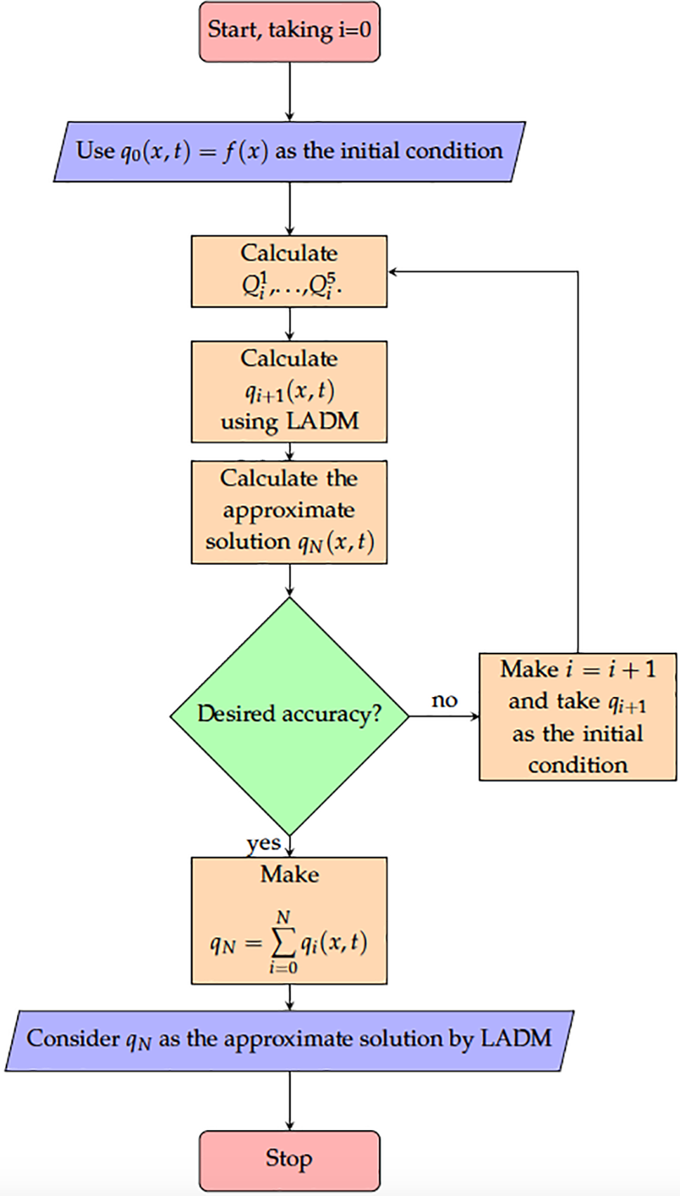
Figure 1: Numerical flow chart

In reference to the application of Eq. (29), the differential equation that was being investigated was subsequently changed into a remarkable identification of elements that could be computed. Following the identification of these parts, we proceed to incorporate them into the Eq. (18) in order to get the final result in form of a series.

A great number of studies have shown that if a problem has a solution that is explicit, then the series that corresponds to that problem will quickly converge at the solution. A number of the authors conducted an in-depth investigation of the idea of convergence in decomposition series in order to provide evidence that the series that was produced converged rather quickly indeed. Cherruault examined the convergence of Adomian’s method in [22]. In addition to that, Cherruault and Adomian [23] gave an original demonstration of convergence for the mentioned approach. For further information about the proofs demonstrating rapid convergence, the reader is directed to the aforementioned sources and the references included therein. Refer to [25] for further details about the approach and its specific relevance to solitary waves. An enhancement of Adomian’s method has been employed to successfully replicate highly dispersive solitons, which include both dark, bright, and singular varieties, as recently reported in [26].

4  Method Application

4.1 Simulation of Bright Solitons and Graphical Representations

This part presents the numerical evaluation of the solution for Eq. (1) concerning bright solitons, using LADM with the starting condition at t=0 derived from Eq. (2).

q(x,0)=A1(sech⁡[B1(x)])ei(−κx+Θ).(30)

We now conduct the simulation of the three scenarios outlined in Table 1, with the results and corresponding absolute errors shown in the Figs. 2–4.

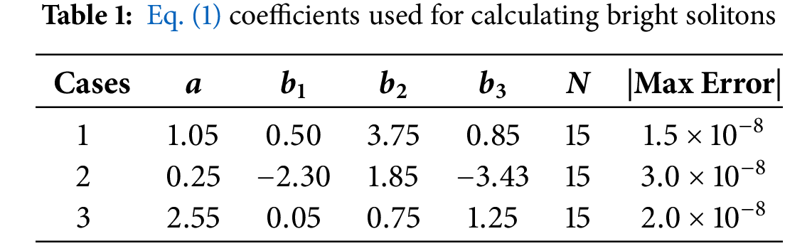
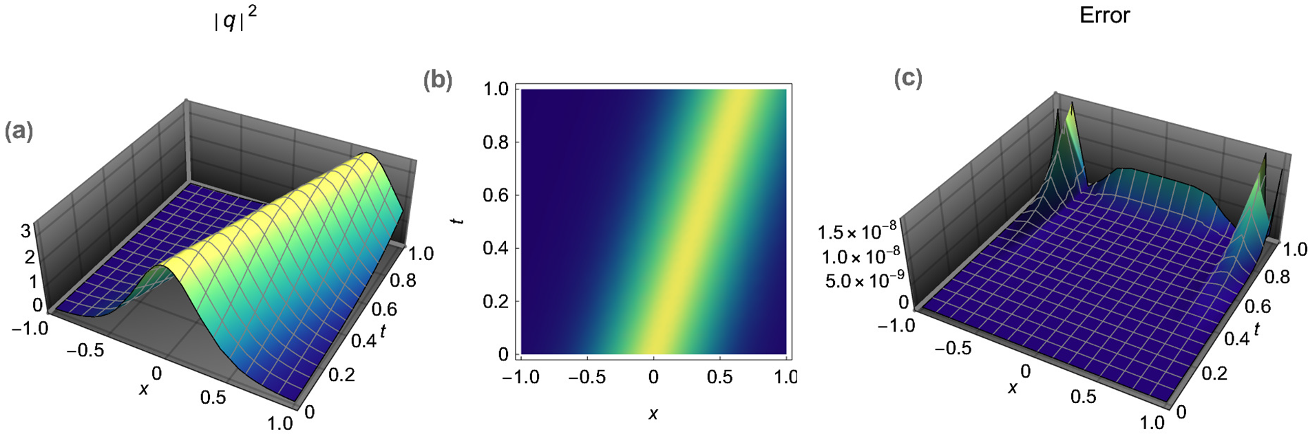
Figure 2: (a) Numerically estimated three-dimensional bright soliton, (b) related two-dimensional density plot, (c) visualize the absolute error as a space-time graph for the 15th iteration related to Case 1 with LADM

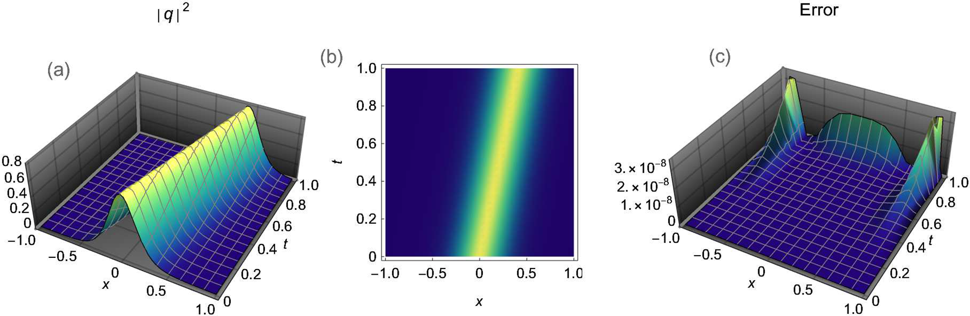
Figure 3: (a) Numerically estimated three-dimensional bright soliton, (b) related two-dimensional density plot, (c) visualize the absolute error as a space-time graph for the 15th iteration related to Case 2 with LADM

Figure 4: (a) Numerically estimated three-dimensional bright soliton, (b) related two-dimensional density plot, (c) visualize the absolute error as a space-time graph for the 15th iteration related to Case 3 with LADM

4.2 Simulation of Dark Solitons and Graphical Representations

This part presents the numerical evaluation of the solution for Eq. (1) concerning dark solitons, using LADM with the starting condition at t=0 derived from Eq. (8).

q(x,0)=A2(tanh⁡[B2(x)])ei(−κx+Θ).(31)

The simulation of the three cases enumerated in Table 2 is now conducted, and the results and their respective absolute errors are illustrated in Figs. 5–7.

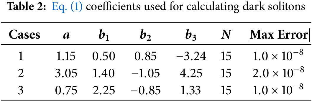
Figure 5: (a) Numerically estimated three-dimensional dark soliton, (b) related two-dimensional density plot, (c) visualize the absolute error as a space-time graph for the 15th iteration related to Case 4 with LADM

Figure 6: (a) Numerically estimated three-dimensional dark soliton, (b) related two-dimensional density plot, (c) visualize the absolute error as a space-time graph for the 15th iteration related to Case 5 with LADM

Figure 7: (a) Numerically estimated three-dimensional dark soliton, (b) related two-dimensional density plot, (c) visualize the absolute error as a space-time graph for the 15th iteration related to Case 6 with LADM

5  Conclusions

This work presents a competitive method compared to other decomposition techniques, utilizing the Laplace transform instead of the integration of increasingly higher-order polynomials. This approach results in an elegant and straightforward method that significantly reduces the computational effort required. In conclusion, it is important to note that the current method exhibits certain deficiencies. Specifically, it yields a series solution that often requires truncation when an analytic solution cannot be identified. Additionally, the region where the ADM solution converges to the exact solution (and consequently where the LADM also converges) is restricted, typically characterized by rapid convergence. To achieve convergence of the solution in a sufficiently large region, it is necessary to incorporate additional terms in the ADM series solution or to employ decomposition methods defined by segments of the interval of interest.

The study recovered bright and dark optical soliton solution to the nonlinear Schrödinger’s equation that came with parabolic and nonlocal nonlinearity forms of self-phase modulation structure. The surface plots, contour plots as well as the error plots that came up after the application of the LADM scheme are displayed. These results from computational quantum optics will be a profound contribution to this field. The displayed results thus stand on a strong footing for further future research with these preliminary foundation. The model will be later addressed with polarization mode dispersion as well as with differential group delay. Those results are currently awaited and will be disseminated across various journals once available.

Acknowledgement: The authors express their gratitude to the anonymous reviewer for their insightful revision suggestions. The corresponding author (AB) is thankful to Grambling State University for the financial support he received as the Endowed Chair of Mathematics.

Funding Statement: The authors received no specific funding for this study.

Author Contributions: Oswaldo González-Gaxiola: Conceptualization, Methodology, Formal analysis, Writing—original draft; Anjan Biswas: Conceptualization, Supervision, Project administration, Funding acquisition, Writing—review; Ahmed H. Arnous: Investigation, Data curation, Validation; Yakup Yildirim: Investigation, Software, Supervision, Visualization, Writing—original draft, Writing—review & editing. All authors reviewed the results and approved the final version of the manuscript.

Availability of Data and Materials: Not applicable.

Ethics Approval: Not applicable.

Conflicts of Interest: The authors declare no conflicts of interest to report regarding the present study.

References

1. Zabusky NJ, Kruskal MD. Interaction of “solitons” in a collisionless plasma and the recurrence of initial states. Phys Rev Lett. 1965;15(6):240–3. doi:10.1103/PhysRevLett.15.240. [Google Scholar] [CrossRef]

2. Hasegawa A, Tappert F. Transmission of stationary nonlinear optical pulses in dispersive dielectric fibers I. Anomalous Dispersion Appl Phys Lett. 1973;23(3):142–4. doi:10.1063/1.1654836. [Google Scholar] [CrossRef]

3. Hasegawa A, Tappert F. Transmission of stationary nonlinear optical pulses in dispersive dielectric fibers II. Normal Dispersion Appl Phys Lett. 1973;23(4):171–2. doi:10.1063/1.1654847. [Google Scholar] [CrossRef]

4. Cohen O, Buljan H, Schwartz T, Fleischer JW, Segev M. Incoherent solitons in instantaneous nonlocal nonlinear media. Phys Rev E. 2006;73(1):015601. doi:10.1103/PhysRevE.73.015601. [Google Scholar] [PubMed] [CrossRef]

5. Zitelli M. Optical solitons in multimode fibers: recent advances. J Opt Soc Am B. 2024;41(8):1655. doi:10.1364/JOSAB.528242. [Google Scholar] [CrossRef]

6. Adomian G, Rach R. On the solution of nonlinear differential equations with convolution product nonlinearities. J Math Anal Appl. 1986;114(1):171–5. doi:10.1016/0022-247X(86)90074-0. [Google Scholar] [CrossRef]

7. Ngartera L, Moussa Y. Advancements and applications of the Adomian decomposition method in solving nonlinear differential equations. J Math Res. 2024;16(4):1–38. doi:10.5539/jmr.v16n4p1. [Google Scholar] [CrossRef]

8. Saddique G, Zeb S, Ali A. Solitary wave solution of Korteweg-De Vries equation by double Laplace transform with decomposition method. Int J Appl Comput Math. 2025;11(1):8. doi:10.1007/s40819-024-01813-6. [Google Scholar] [CrossRef]

9. Biswas A, Rezazadeh H, Mirzazadeh M, Eslami M, Zhou Q, Moshokoa SP, et al. Optical solitons having weak non-local nonlinearity by two integration schemes. Optik. 2018;164(5):380–4. doi:10.1016/j.ijleo.2018.03.026. [Google Scholar] [CrossRef]

10. Mirzazadeh M, Hosseini K, Dehingia K, Salahshour S. A second-order nonlinear Schrödinger equation with weakly nonlocal and parabolic laws and its optical solitons. Optik. 2021;242:166911. doi:10.1016/j.ijleo.2021.166911. [Google Scholar] [CrossRef]

11. Zhou Q, Yao DZ, Chen F. Analytical study of optical solitons in media with Kerr and parabolic-law nonlinearities. J Mod Opt. 2013;60(19):1652–7. doi:10.1080/09500340.2013.852695. [Google Scholar] [CrossRef]

12. Hosseini K, Salahshour S, Mirzazadeh M. Bright and dark solitons of a weakly nonlocal Schrödinger equation involving the parabolic law nonlinearity. Optik. 2021;227:166042. doi:10.1016/j.ijleo.2020.166042. [Google Scholar] [CrossRef]

13. Akinyemi L, Şenol M, Mirzazadeh M, Eslami M. Optical solitons for weakly nonlocal Schrödinger equation with parabolic law nonlinearity and external potential. Optik. 2021;230(1-2):166281. doi:10.1016/j.ijleo.2021.166281. [Google Scholar] [CrossRef]

14. Alngar ME, Mostafa AM, AlQahtani SA, Shohib RM, Pathak P. Highly dispersive eighth-order embedded solitons with cubic-quartic χ(2) and χ(3) nonlinear susceptibilities under the influence of multiplicative white noise using Itô calculus. Modern Physics Letters B. 2024;2450474. doi:10.1142/S0217984924504748. [Google Scholar] [CrossRef]

15. Alngar ME, Alamri AM, AlQahtani SA, Shohib RM, Pathak P. Exploring optical soliton solutions in highly dispersive couplers with parabolic law nonlinear refractive index using the extended auxiliary equation method. Mod Phys Lett B. 2024;38(34):2450350. doi:10.1142/S0217984924503500. [Google Scholar] [CrossRef]

16. Kai Y, Yin Z. Linear structure and soliton molecules of Sharma-Tasso-Olver-Burgers equation. Phys Lett A. 2022;452(15):128430. doi:10.1016/j.physleta.2022.128430. [Google Scholar] [CrossRef]

17. He Y, Kai Y. Wave structures, modulation instability analysis and chaotic behaviors to Kudryashov’s equation with third-order dispersion. Nonlinear Dyn. 2024;112(12):10355–71. doi:10.1007/s11071-024-09635-3. [Google Scholar] [CrossRef]

18. Adomian G. Solving frontier problems of physics: the decomposition method. Boston, MA, USA: Kluwer Academic Publishers; 1994. [Google Scholar]

19. Chen W, Lu Z. An algorithm for Adomian decomposition method. Appl Math Comput. 2004;158(1):221–35. doi:10.1016/j.amc.2003.10.037. [Google Scholar] [CrossRef]

20. Mohammed ASHF, Bakodah HO. Numerical investigation of the Adomian-based methods with w-shaped optical solitons of Chen-Lee-Liu equation. Phys Scr. 2021;96(3):035206. doi:10.1088/1402-4896/abd0bb. [Google Scholar] [CrossRef]

21. Duan JS. Convenient analytic recurrence algorithms for the Adomian polynomials. Appl Math Comput. 2011;217(13):6337–48. doi:10.1016/j.amc.2011.01.007. [Google Scholar] [CrossRef]

22. Cherruault Y. Convergence of Adomian’s method. Kybernetes. 1989;18(2):31–8. doi:10.1108/eb005812. [Google Scholar] [CrossRef]

23. Cherruault Y, Adomian G. Decomposition methods: a new proof of convergence. Math Comput Modelling. 1993;18(2):103–6. doi:10.1016/0895-7177(93)90233-O. [Google Scholar] [CrossRef]

24. Duan JS, Rach R, Wazwaz AM. A new modified Adomian decomposition method for higher-order nonlinear dynamical systems. Comput Model Eng Sci. 2013;94(1):77–118. doi:10.3970/cmes.2013.094.077. [Google Scholar] [CrossRef]

25. Wazwaz AM. Partial differential equations and solitary waves theory. Berlin/Heidelberg: Springer-Verlag; 2009. [Google Scholar]

26. Qarni AAA, Bodaqah AM, Mohammed ASHF, Alshaery AA, Bakodah HO, Biswas A. Dark and singular cubic-quartic optical solitons with Lakshmanan-Porsezian-Daniel equation by the improved Adomian decomposition scheme. Ukr J Phys Opt. 2023;24(1):46–61. doi:10.3116/16091833/24/1/46/2023. [Google Scholar] [CrossRef]