
 Submit a Paper
 Propose a Special lssue
 Open Access
ARTICLE
Computational Modeling of Streptococcus Suis Dynamics via Stochastic Delay Differential Equations
1 Department of Mathematics, National College of Business Administration and Economics, Lahore, 54000, Pakistan
2 Center for Research in Mathematics and Applications (CIMA), Institute for Advanced Studies and Research (IIFA), University of Évora, Rua Romão Ramalho, 59, Évora, 7000-671, Portugal
3 Department of Computer Science and Mathematics, Lebanese American University, Beirut, 1102-2081, Lebanon
4 Department of Zoology, University of Sialkot, Sialkot, 51040, Pakistan
5 Department of Mathematics, Air University, Islamabad, 44000, Pakistan
6 Department of Mathematics and Statistics, College of Science, King Faisal University, Al Ahsa, 31982, Saudi Arabia
7 Department of Physical Sciences, The University of Chenab, Gujrat, 50700, Pakistan
* Corresponding Authors: Ali Raza. Email: ,
; Emad Fadhal. Email:
(This article belongs to the Special Issue: Advances in Mathematical Modeling: Numerical Approaches and Simulation for Computational Biology)
Computer Modeling in Engineering & Sciences 2025, 143(1), 449-476. https://doi.org/10.32604/cmes.2025.061635
Received 29 November 2024; Accepted 05 February 2025; Issue published 11 April 2025
 View Full Text
 Download PDF
Abstract
Streptococcus suis (S. suis) is a major disease impacting pig farming globally. It can also be transferred to humans by eating raw pork. A comprehensive study was recently carried out to determine the indices through multiple geographic regions in China. Methods: The well-posed theorems were employed to conduct a thorough analysis of the model’s feasible features, including positivity, boundedness equilibria, reproduction number, and parameter sensitivity. Stochastic Euler, Runge Kutta, and Euler Maruyama are some of the numerical techniques used to replicate the behavior of the streptococcus suis infection in the pig population. However, the dynamic qualities of the suggested model cannot be restored using these techniques. Results: For the stochastic delay differential equations of the model, the non-standard finite difference approach in the sense of stochasticity is developed to avoid several problems such as negativity, unboundedness, inconsistency, and instability of the findings. Results from traditional stochastic methods either converge conditionally or diverge over time. The stochastic non-negative step size convergence nonstandard finite difference (NSFD) method unconditionally converges to the model’s true states. Conclusions: This study improves our understanding of the dynamics of streptococcus suis infection using versions of stochastic with delay approaches and opens up new avenues for the study of cognitive processes and neuronal analysis. The plotted interaction behaviour and new solution comparison profiles.Keywords
In [1], the authors provide a mathematical model for streptococcus suis infection in the pig population. The technique used to evaluate the model is beneficial for overcoming the disease. In [2], the authors constructed a factual model to regulate model specifications in several antibiotic ramifications various perceptions, and instructions of infection to resist streptococcus suis. In [3], the authors studied separately from recently discovered streptococcus suis species. In [4], the author’s presence of streptococcus suis illness in seedling pigs was linked to pigs that performed averagely and had a sow effect rather than any notable disease traits. In [5], the authors’ enhanced infection was only seen in the upper respiratory tract in this investigation. We used two separate models to assess the variations in streptococcus suis disease. In [6], the authors provide more convincing evidence for the beneficial effects of the drug vs. streptococcus suis disease by elucidating the underlying molecular process. In [7], the authors evaluate the effect of implementing an autogenous vaccination program on the emergence of illnesses linked to streptococcus suis in natural environments as a challenging undertaking. In [8], the authors illustrate that the survival of other streptococcus suis pathotypes in porcine blood is also restricted by antibody-mediated, as evidenced by the fact that the bacterial surface was usually substantially greater following development in standard piglets’ plasma than following incubation in serum obtained before any colostrum adoption. In [9], the authors are shown to be the most effective solvent for a substance called separation by ultrasound-assisted extraction (UAE), and the response surface methodology (RSM) framework accurately represented the anticipated optimization of Emirati. In [10], the authors discovered during the streptococcus suis-2 disease, vimentin increased lung damage, neutrophil counts, and the production of proinflammatory cytokines and chemokines in the lungs of pigs and swine tracheal epithelial cells (STEC). In [11], the authors illustrate how the host-defense peptide cathelicidins are avoided by the Streptococcus suis pepo protease, which affects the pathophysiology of Streptococcus suis. It was discovered that Pepo cleaves the anti-Streptococcus suis cathelicidins, mouse cathelicidin mouse and human cathelicidin. In [12], the authors present the mathematical framework of climate influence on Streptococcus suis infection in pig-human populations generally. In [13], the authors developed a fractional-order mathematical framework relying on fractional derivative concepts. In [14], the authors’ investigation is based on the hypotheses of further studies in this domain, especially utilizing both experimental and real-world data. The model suggested that batch-level isolation might cause a likelihood of Streptococcus suis incidence in the facility. In [15], the authors studied that Streptococcus suis is a human pathogen that is frequently responsible for meningitis in Asian nations that consume pork. In [16], the authors provide an exclusive preventative option accessible to pig breeders as a possibility to medicines for controlling the Streptococcus suis infection. In [17], the authors determine that Streptococcus suis strain extracted from an appropriate pig tonsil is aggressive and possesses multiple mechanisms that encourage niche conflict in pig tonsil. In [18], the authors create a computational model of Streptococcus suis infection in a pig community. The approach employed to analyze the model is useful in conquering the illness. In [19], the authors examine blood cortisol levels as a distress readout metric and buprenorphine therapy as a refining measure in a novel pig Streptococcus suis disease model. In [20], the authors created a scientific simulation to control model parameters in several antibiotic implications, different perspectives on infection, and guidelines for resisting Streptococcus suis. In [21], the author explores the use of Stochastic Differential Equations (SDEs) in applications of sciences and many more. In [22], the authors studied the existence and approximate controllability of the Hilfer fractional neutral stochastic hemivariational inequality with the Rosenblatt process. Stochastic or probabilistic components are included in a mathematical model of Streptococcus suis infection dissemination by numerical simulation and analysis, with an emphasis on accounting for uncertainty in disease transmission. Public health efforts for disease control and prevention are informed by this kind of modeling, which provides insights into how the illness could spread under various circumstances.
The main key point to study is the structure-preserving and dynamical analysis of the Streptococcus suis disease model. The fundamental properties of the model like positivity, boundedness, and local and global stabilities are studied rigorously. The authors used well-known methods like Euler Maruyama, stochastic Euler, and stochastic Runge Kutta for the computational analysis and made a comparison analysis with the proposed method like nonstandard finite difference in the sense of stochastic. The Nonstandard Finite Difference (NSFD) method gives a guarantee of Structure-preserving properties of the model like positivity, boundedness, and dynamical consistency of the solution instead of other standard methods.
The paper is organized as follows: An overview of Streptococcus suis infection-like conditions and a thorough assessment of the literature is provided in Section 1. Building the delayed model and the ensuing mathematical analysis are the focus of Section 2. In Section 3, the local and global levels of the model’s stability, reproduction number, and equilibria are examined. The sensitivity analysis of the model’s parameters is covered in Section 4. The stochastic conceptualization phase is presented in Section 5. The numerical approach of the NSFD technique and numerical simulations and the presentation of the results are the explicit focus of Section 6. Final opinions provide a conclusive overview of the work under Section 7.
This section presents the delay model formulation of infection spread by pigs and humans. Four classifications were used to categorize the pig population: susceptible class
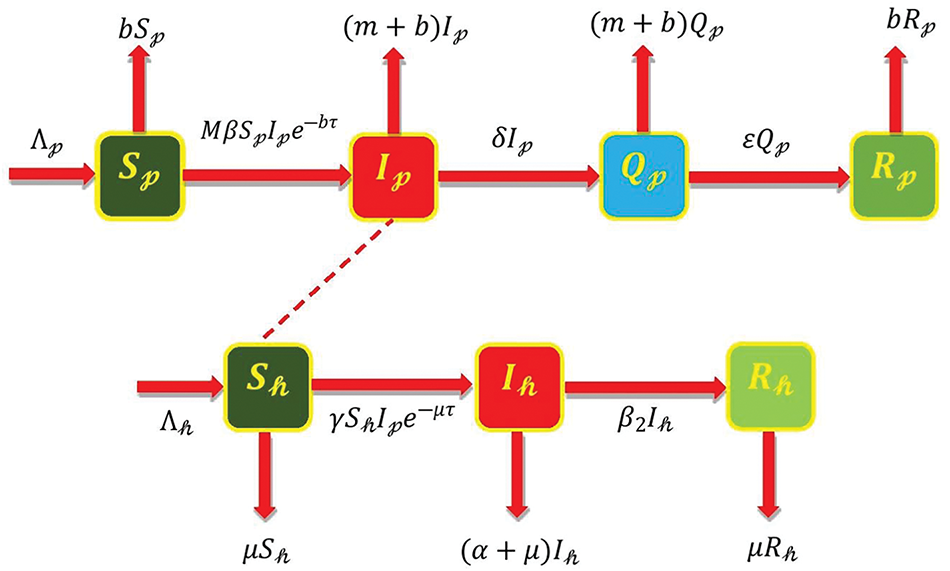
Figure 1: SIQR-SIR model diagram for people and pigs [13]
By
The pig model attribute can be expressed as follows:
This section examines the delay model feasible region, which carries biological significance as the suggested model takes into account. Consider every parameter and variable in the delay model is non-negative. Next, the model’s equilibria and the fundamental reproduction number are determined. Furthermore, we investigate each equilibrium at locally and globally stable.
The feasible region of the system (1)–(7) is shown
Theorem 1: The solution of the system (1)–(7) is positive in the feasible region.
Proof: Consider the system (1)–(7), we have
Hence, system (1)–(7) has a positive solution with the initial condition in the feasible region. □
Theorem 2: The solution of the model (1)–(7) is bounded in the feasible region.
Proof: The total number of people and pigs may be written as
Which is a linear differential equation
Using Grown’s inequality
3.2 Model Equilibria and Reproduction Number
This section includes two types of model equilibria for Streptococcus Suis Equilibrium.
Streptococcus Suis Endemic Equilibrium
The reproduction number is vastly essential in epidemiology. This determines the probability that the illness exists in the community or not. If the reproduction is less than one, disease can be prevented in the community; if the reproduction number is larger than one, disease exists in the community. Use the next-generation approach to calculate the reproduction number. Thus,
The largest eigenvalue of the matrix called the spectral radius or reproduction number at Streptococcus suis free equilibrium, follows as
We will demonstrate the following well-known result about local and global stability in both model equilibrium points. Consider the function as follows:
The Jacobian matrix has the following elements:
Theorem 3: The Streptococcus Suis Free Equilibrium
Proof: For stability at
Hence the streptococcus Suis free equilibrium of the given system (1)–(7) is stable in the sense of local if
Theorem 4: The Streptococcus Suis Endemic Equilibrium
Proof: Letting from (8), we get
For eigenvalue, consider
So, by the Routh-Hurwitz Criterion for a 2nd-degree polynomial, the coefficient of the characteristic equation is positive with the constraint
The stability of the Streptococcus Suis infection model is demonstrated by well-known outcomes in following global sense.
Theorem 5: The Streptococcus Suis Free Equilibrium
Proof: Define the Volterra Lyapunov function
This implies that
Theorem 6: The Streptococcus suis Endemic Equilibrium
Proof: Define the Volterra Lyapunov function
Given positive constants
If we choose
Theorem 7. The Streptococcus suis Free Equilibrium
Proof: Define the Volterra Lyapunov function
Thus, the system (1)–(7) is globally asymptotically stable at Streptococcus Suis Free Equilibrium. □
Theorem 8. The Streptococcus Suis Endemic Equilibrium
Proof: Define the Volterra Lyapunov function
For simplification, we choose
It can see that
This section examined the streptococcus suis model’s sensitivity. Sensity analysis is a study of how various factors related to input uncertainty may be attributed to the inconsistency of a mathematical model’s output outcomes. We calculate the sensitivity of the reproduction number concerning the model’s parameter. This technique provided the most sensitive measure for the reproduction number, which helped the infection spread. The basic format for sensitivity is as follows:
where
The values of sensitivity and signs of the model’s parameters are presented in Table 1.

The most significant contributing aspect to the viral transmission phenomenon is human morality (
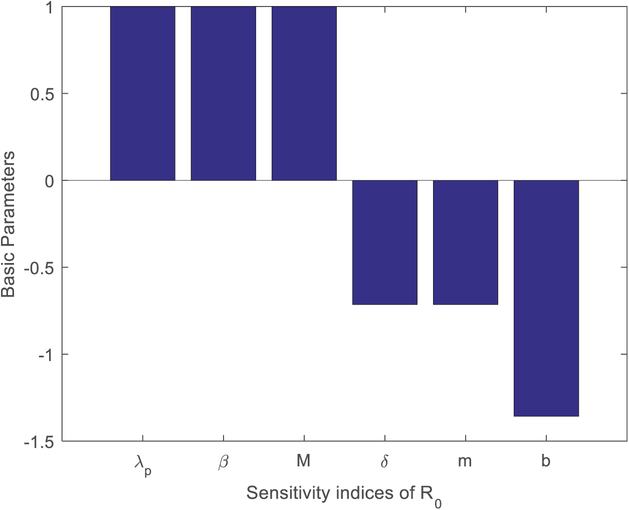
Figure 2: Analysis of the sensitive indices of reproduction number
5 Stochastic Formulation Phase 1
The Stochastic delayed differential equations (SDDEs) of the streptococcus suis model (1)–(7) may be represented by the vector
Therefore,
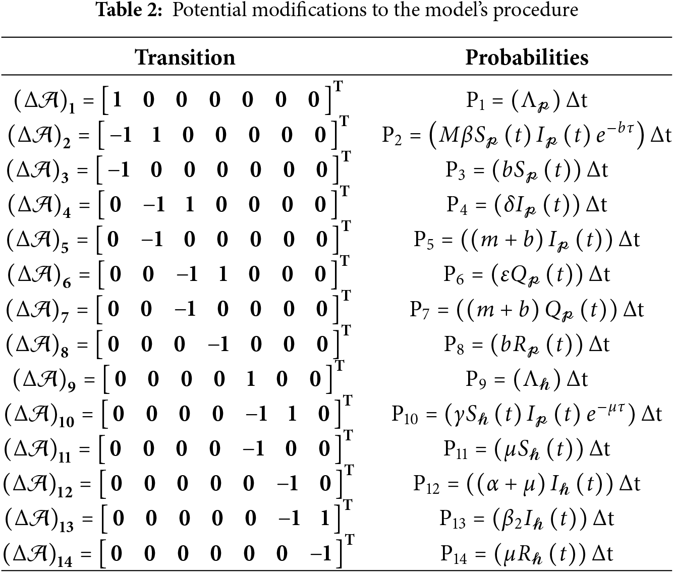
By studying the relevant academic literature, the Euler Maruyama approach is employed to simulate the results of Eq. (10). Following is an outline of the data that is shown in Table 2.
where the discretization parameter is denoted by
5.1 Stochastic Formulation Phase 2
Create an uncertainty parameter for the dynamical system (1)–(7) by including Brownian motion.
where
5.2 Fundamental Properties of the Stochastic Model
This part covers the analysis of the positivity and boundedness properties of the system (11)–(17).
Let us consider the vector as follows:
and norm
And
Furthermore, let
As
And
If
where T is Transportation.
Theorem 9 Shows that for the system (11)–(17) and any given initial conditions
Proof. Given that all model parameters satisfy the local Lipschitz limitations. Thus, according to Ito’s formula, the provided model has a positive solution locally on the interval
Let
where we set
The inequality states that
If this condition fails to be satisfied, then there exist values T > 0 and
Define a
Define a
By using Ito’s formula (25), we calculate
For simplify, we assume
where
where
Set
For each element
Next, we obtain
The indicator function is denoted as
As desired.
Again, by using Ito’s formula (26), we calculate
For simplify, we assume
where
where
Hence,
Next, we obtain
The indicator function is denoted as
As desired. □
Theorem 10. If the spectral radius v and the variance
Proof: Let’s examine the initial data
Applying Ito’s lemma to the function f(
Notice that,
If
If
6 Stochastic Nonstandard Finite Difference Scheme
The NSFD method is used in this analysis to address the stochastic delay differential equations regulating Streptococcus suis dynamics. The discrete approximations are very carefully selected to keep stability and be able to precisely model the turbulent behavior of the system. This ensures that the theoretical analysis is kept consistent and that the numerical solutions stay physically significant. For (11)–(17), the stochastic non-standard finite difference scheme has the following equation:
where
Assuming
The Jacobian matrix consists of the following elements:
Theorem 11. For all values of
Proof. The Jacobian matrix at the streptococcus suis-free equilibrium, denoted as
Therefore,
Using the definition of
Theorem 12. For all values of
Proof. The Jacobian matrix at the streptococcus suis- endemic equilibrium, denoted as
So, the eigenvalues of the Jacobian at
Lemma. For the quadratic equation
(i)
(ii)
(iii)
This section examines the characteristics of the graphs representing the number of infected pig population using the Euler Maruyama, stochastic Euler, and stochastic Runge Kutta schemes, in comparison to the NSFD scheme, across various step sizes and parameters values (See Table 3).
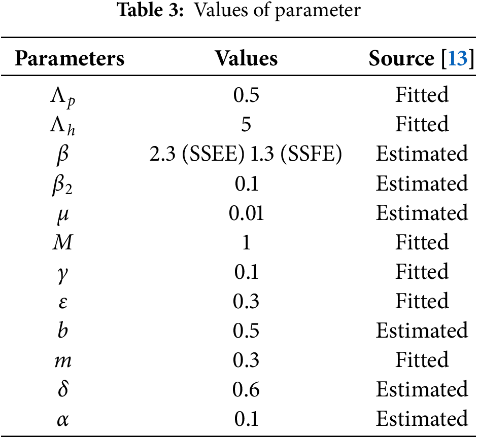
Fig. 3a,b provides a comparison between the infected class of the Stochastic NSFD and the Euler Maryama Method. Fig. 3a shows convergence for both approaches at ℎ = 0.01. When the step size was raised to ℎ = 1.0, the Euler Maryama Method diverged whereas the Stochastic NSFD Method remained convergent, as shown in Fig. 3b. Similarly, Fig. 3c,d compares the infected class of the Stochastic NSFD and the Stochastic Euler Method. At ℎ = 0.01, both techniques converged in Fig. 3c. However, when the step size was increased to ℎ = 1.0, the Stochastic Euler Method diverged, while the Stochastic NSFD method-maintained convergence, as shown in Fig. 3d. Similarly, Fig. 3e,f compares the infected class of the Stochastic NSFD and Stochastic RK Method. At ℎ = 0.01, both methods converged, as shown in Fig. 3e. However, when the step size increased to ℎ = 2.0, the Stochastic RK Method diverged, while the Stochastic NSFD method continued to converge, as shown in Fig. 3f. Fig. 4a shows how delay affects the model’s susceptible class at different ???? values (0.1, 0.2, 0.3, 0.4, 0.5). Fig. 4b shows the effect of delay on the infected class of the model at various values ???? = 0.1, 0.2, 0.3, 0.4, and 0.5, indicating a gradual decline in disease from the infected class over time. Finally, Fig. 5 shows the behavior of delay on the reproduction number of the model.

Figure 3: Comparison graph of computational methods at the Streptococcus Suis endemic equilibrium of the model (a) The comparison behavior of the infected pig population through Euler Maruyama and stochastic NSFD methods at

Figure 4: Time-Plot with the time delay on susceptible and infected population. (a) The effect of different values of delay on susceptible pig population (b) The effect of different values of delay on infected pig population
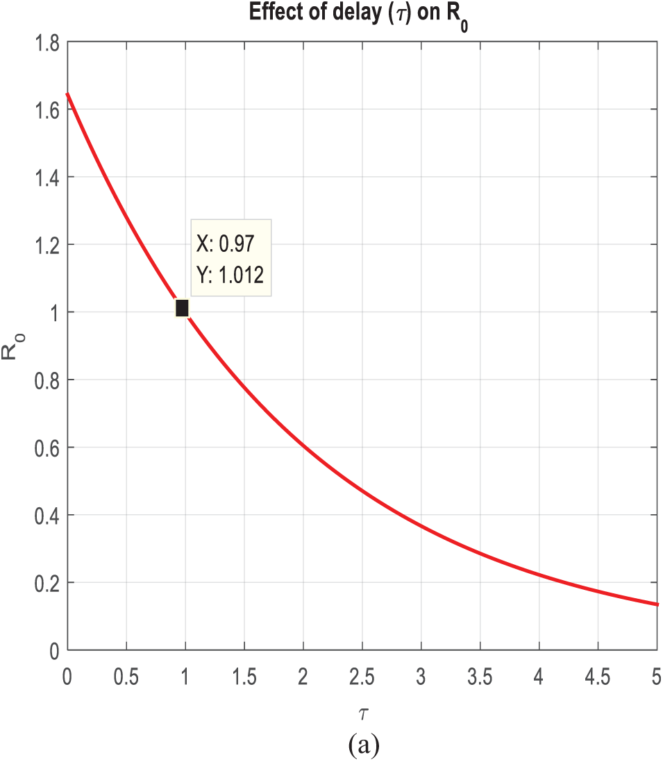
Figure 5: Time plot of the effect of time delay
This paper provides a comprehensive assessment of the mathematical analysis, including trustworthy delay techniques, of the delayed model for streptococcus suis infection. Subpopulations are classified by the model into four categories: susceptible class
To fully capture the real-world complexities, there is a need to develop a model without the assumption of disease transmissibility and parameter estimation. Moreover, validation based on data is needed to enhance the reliability of the model.
Acknowledgement: Not applicable.
Funding Statement: This work was supported by the Deanship of Scientific Research, Vice Presidency for Graduate Studies and Scientific Research, King Faisal University, Saudi Arabia [KFU250259].
Author Contributions: Umar Shafique, Ali Raza, Dumitru Baleanu, Khadija Nasir, Muhammad Naveed, Abu Bakar Siddique and Emad Fadhal reviewed the results and approved the final version of the manuscript. All authors reviewed the results and approved the final version of the manuscript.
Availability of Data and Materials: All the data used and analyzed is available in the manuscript.
Ethics Approval: Not applicable.
Conflicts of Interest: The authors declare no conflicts of interest to report regarding the present study.
References
1. Alqahtani AM, Mishra MN. Mathematical analysis of Streptococcus suis infection in pig-human population by Riemann-Liouville fractional operator. Progr Fract Diff Appl. 2024;10(1):119–35. doi:10.18576/pfda/100112.
2. Mi K, Sun L, Zhang L, Tang A, Tian X, Hou Y, et al. A physiologically based pharmacokinetic/pharmacodynamic model to determine dosage regimens and withdrawal intervals of aditoprim against Streptococcus suis. Front Pharmacol. 2024;15:1378034. doi:10.3389/fphar.2024.1378034.
3. Wu CF, Chen SH, Chou CC, Wang CM, Huang SW, Kuo HC. Serotype and multilocus sequence typing of Streptococcus suis from diseased pigs in Taiwan. Sci Rep. 2023;13(1):8263. doi:10.1038/s41598-023-33778-9.
4. Fabà L, Aragon V, Litjens R, Galofré-Milà N, Segura M, Gottschalk M, et al. Metabolic insights and background from naturally affected pigs during Streptococcus suis outbreaks. Transl Anim Sci. 2023;7(1):txad126. doi:10.1093/tas/txad126.
5. Hau SJ, Nielsen DW, Brockmeier SL. Prior infection with Bordetella bronchiseptica enhanced colonization but not disease with Streptococcus suis. Vet Microbiol. 2023;284(4):109841. doi:10.1016/j.vetmic.2023.109841.
6. Lou F, Huang H, Li Y, Yang S, Shi Y. Investigation of the inhibitory effect and mechanism of epigallocatechin-3-gallate against Streptococcus suis sortase A. J Appl Microbiol. 2023;134(9):lxad191. doi:10.1093/jambio/lxad191.
7. Jeffery A, Gilbert M, Corsaut L, Gaudreau A, Obradovic MR, Cloutier S, et al. Immune response induced by a Streptococcus suis multi-serotype autogenous vaccine used in sows to protect post-weaned piglets. Vet Res. 2024;55(1):1–21. doi:10.1186/s13567-024-01313-x.
8. Zhu H, Müller U, Baums CG, Öhlmann S. Comparative analysis of the interactions of different Streptococcus suis strains with monocytes, granulocytes and the complement system in porcine blood. Vet Res. 2024;55(1):14. doi:10.1186/s13567-024-01268-z.
9. Bai J, Xie Y, Li M, Huang X, Guo Y, Sun J, et al. Ultrasound-assisted extraction of emodin from Rheum officinale Baill and its antibacterial mechanism against Streptococcus suis based on CcpA. Ultrason Sonochem. 2024;102:106733. doi:10.1016/j.ultsonch.2023.106733.
10. Meng Y, Lin S, Niu K, Ma Z, Lin H, Fan H. Vimentin affects inflammation and neutrophil recruitment in airway epithelium during Streptococcus suis serotype 2 infection. Vet Res. 2023;54(1):7. doi:10.1186/s13567-023-01135-3.
11. Jin M, Liang S, Wang J, Zhang H, Zhang Y, Zhang W, et al. Endopeptidase O promotes Streptococcus suis immune evasion by cleaving the host-defence peptide cathelicidins. Virulence. 2023;14(1):2283896. doi:10.1080/21505594.2023.2283896.
12. Chaiya I, Trachoo K, Nonlaopon K, Prathumwan D. The mathematical model for streptococcus suis infection in pig-human population with humidity effect. Comput Mater Contin. 2022;71(2):2981–98. doi:10.32604/cmc.2022.021856.
13. Prathumwan D, Chaiya I, Trachoo K. Study of transmission dynamics of Streptococcus suis infection mathematical model between pig and human under ABC fractional-order derivative. Symmetry. 2022;14(10):2112. doi:10.3390/sym14102112.
14. Giang E, Hetman BM, Sargeant JM, Poljak Z, Greer AL. Examining the effect of host recruitment rates on the transmission of Streptococcus suis in nursery swine populations. Pathogens. 2020;9(3):174. doi:10.3390/pathogens9030174.
15. Arenas Jús, Zomer A, Harders-Westerveen J, Bootsma HJ, De Jonge MI, Stockhofe-Zurwieden N, et al. Identification of conditionally essential genes for Streptococcus suis infection in pigs. Virulence. 2020;11(1):446–64. doi:10.1080/21505594.2020.1764173.
16. Corsaut L, Misener M, Canning P, Beauchamp G, Gottschalk M, Segura M. Field study on the immunological response and protective effect of a licensed autogenous vaccine to control Streptococcus suis infections in post-weaned piglets. Vaccines. 2020;8(3):384. doi:10.3390/vaccines8030384.
17. Liang Z, Wu H, Bian C, Chen H, Shen Y, Gao X, et al. The antimicrobial systems of Streptococcus suis promote niche competition in pig tonsils. Virulence. 2022;13(1):781–93. doi:10.1080/21505594.2022.2069390.
18. Huan H, Jiang L, Tang L, Wang Y, Guo S. Isolation and characterization of Streptococcus suis strains from swine in Jiangsu province. China J Appl Microbiol. 2020;128(6):1606–12. doi:10.1111/jam.14591.
19. Liedel C, Mayer L, Einspanier A, Völker I, Ulrich R, Rieckmann K, et al. A new S. suis serotype 3 infection model in pigs: lack of effect of buprenorphine treatment to reduce distress. BMC Vet Res. 2022;18(1):435. doi:10.1186/s12917-022-03532-w.
20. Tan M‐F, Zou G, Wei Y, Liu W‐Q, Li H‐Q, Hu Q, et al. Protein-protein interaction network and potential drug target candidates of Streptococcus suis. J Appl Microbiol. 2021;131(2):658–70. doi:10.1111/jam.14950.
21. Oksendal B. Stochastic differential equations: an introduction with applications. Springer Science & Business Media; 2013. [cited 2025 Jan 15]. https://link.springer.com/book/10.1007/978-3-642-14394-6.
22. Gokul G, Udhayakumar R. Existence and approximate controllability for the Hilfer fractional neutral stochastic hemivariational inequality with Rosenblatt process. J Contr Decis. 2024;4(50):1–14. doi:10.1080/23307706.2024.2403492.
Cite This Article
 Copyright © 2025 The Author(s). Published by Tech Science Press.
This work is licensed under a Creative Commons Attribution 4.0 International License , which permits unrestricted use, distribution, and reproduction in any medium, provided the original work is properly cited.
 Downloads
 Citation Tools