Heat Transfer Area Optimization for Heat Exchanger System

1  Introduction

Using tolerance optimization to design systems susceptible to parameter variations is very important in parameter design optimization. Traditional parameter design often assumes that parameters can be precisely realized and remain constant during operation. However, this ignores the fluctuations and uncertainties that may exist in real-world environments. In this case, even minor deviations can lead to significant degradation of system performance. Therefore, the purpose of tolerance-optimized design is to consider these variations and ensure the system remains robust within the permitted range.

Two types of tolerance design methods are commonly used to deal with changes in operating parameters and parameter specifications: robust parameter design and optimization design methods. Robust parameter design minimizes external factors’ effects on product quality so that the product remains of high quality even under less-than-ideal environmental conditions [1]. The Taguchi method is a method to obtain robust parameters in heat exchanger systems [2–4]. However, this method only considers tolerance design. Although robust parameter values can be obtained, it may not be possible to ensure that the system’s overall performance is optimal. Optimization design methods use optimization algorithms to find the best parameter values to improve the system performance [5]. However, they usually ignore the robustness of these parameters to external variations or errors, resulting in a lack of robustness of the best parameters in a fluctuating environment.

A heat exchanger system is used to transfer heat between fluids of different temperatures. This system is commonly used in petroleum, chemical, metallurgy, power, light, food, and other industries [6]. The most common criteria for heat exchanger optimization are minimum initial cost, minimum operating cost, maximum efficiency, minimum pressure drop, minimum heat transfer area, and minimum weight or material [7]. Venkatesh et al. used a multi-objective genetic algorithm to solve the complex decision problem of cost, thermal resistance, and ultimate utility of heat exchanger systems [8]. Bianco et al. used a multi-objective genetic algorithm to minimize the heat transfer area of heat exchanger systems [9]. Yang et al. used an improved stochastic ranking evolutionary strategy algorithm to minimize the heat transfer area of heat exchanger systems [10]. Rani et al. used multi-objective optimization of opposition learning with beetle swarm algorithm to design a heat exchanger system to reduce five objective functions: total heat transfer rate, total weight, total mass flow rate, number of entropy generating units, and whole annual cost [11]. Gawai et al. used a modified, amended differential evolution algorithm to minimize the heat transfer area of the heat exchanger system [12]. Bakr et al. applied a genetic algorithm to optimize the design of a shell-and-tube heat exchanger to improve its thermal performance by maximizing heat transfer efficiency while minimizing pressure drop [13]. Zhang et al. enhanced the performance of a central heating system by optimizing the distribution of heat transfer area and the mass flow rates of working fluids, aiming to maximize the temperature of the cold fluid as the optimization objective [14]. Kharaji used constrained optimization algorithms to minimize heat transfer areas in shell-and-tube heat exchangers [7]. Shafiey Dehaj et al. applied a genetic algorithm to reduce heat transfer areas and improve the effectiveness of fin and tube heat exchangers [15]. Wu et al. used a genetic algorithm to design the spiral-wound heat exchanger and minimize its heat transfer areas [16]. From the survey of existing literature, many scholars have presented the heat exchanger system for minimizing heat transfer area. However, they assumed no uncertainty in the system’s operating temperature parameters. Therefore, many scholars have assumed a constant value for the system’s operating temperature during the optimization process. In industry, it is difficult to fix a system’s operating temperature at a constant state, and the optimal parameters obtained by assuming a constant value for the system’s operating temperature parameters are bound to have uncertain errors in practical applications [17]. Temperature cannot be accurately measured or controlled at every critical design point. However, this uncontrollable factor can be considered as a disturbance factor and integrated into the overall system design process. Although group search optimization (GSO) has demonstrated numerous successful applications, it suffers from poor search performance—its low accuracy and tendency to become trapped in local optima result in poor robustness. Therefore, Yang et al. used the experimental design approach to solve this problem and verified its performance [10]. However, it lacks tolerance capabilities. Thus, this paper focuses on the optimal design of the uncertainty system operating temperature parameters of the heat exchanger system through an allowable-tolerance-based group search optimization algorithm (AT-GSO) to achieve the minimum heat transfer area. The method proposed in this paper can consider the existence of uncertainty in the system operating temperature during the parameter optimization process, so that it can be applied in practice to reduce the impact caused by the error in the system operating temperature.

2  Problem Statement and Application Methods

2.1 Problem Statement

The heat exchanger is a kind of energy-saving equipment used to achieve heat transfer between materials, but also in the development and utilization of secondary energy, heat recovery, and energy saving of the main equipment. The chemical plant utilizes waste heat from the plant, which uses three heat exchangers to heat the material temperature from 100°C to 500°C. Conventional design methods focus on the optimization of individual heat exchangers, ignoring the interaction between heat exchangers in the heat exchanger network. The superstructure of the heat exchanger system is shown in Fig. 1. This paper investigates how to optimize the system operating temperatures T1 and T2 to minimize the total heat transfer area of the heat exchanger system, where there are uncertainties △T1 and △T2 in the system operating temperature parameters.

Figure 1: The heat exchanger system structure

Neglecting the change of specific heat of each material with temperature, according to the law of conservation of heat for the three heat exchangers, can be calculated as follows [18]:

mcp(T1−100)=mcp(300−T3),(1)

mcp(T2−T1)=mcp(400−T4),(2)

mcp(500−T2)=mcp(600−T5).(3)

Assuming arithmetic mean temperature difference for each heat exchanger yields:

Δtm1=(300−T1) + (T3−100)2=300−T1,(4)

Δtm2=(400−T2) + (T4−T1)2=400−T2,(5)

Δtm3=(600−500) + (T5−T2)2=100.(6)

The heat transfer area can be calculated according to the heat equation as follows:

Ai=QiKiΔtmi=mcpΔTiKiΔtmi,(7)

where i is the number of the heat exchanger, A is the heat transfer area of the heat exchanger, Q is the amount of heat exchanged by the heat exchanger, K is the heat transfer coefficient of the heat exchanger, and △tm is the average value of temperature difference of the heat exchanger.

Thus, the single-objective optimization problem of the total heat transfer area of the heat exchanger system is described as follows [18]:

Minimize A=A1+A2+A3=100000(T1−100)120(300−T1)+100000(T2−T1)80(400−T2)+100000(500−T2)40×100,(8)

where 100 ≤ T1 ≤ 300 and T1 ≤ T2 ≤ 400. The uncertainties △T1 and △T2 in the system operating temperature parameters is between 0% and 40%.

2.2 Allowable-Tolerance Based GSO Algorithm

The Group Search Optimization (GSO) algorithm relies on random searchers (Rangers) to conduct exploitation search operations. A single best-fit producer (Producer) is typically selected to perform exploration searches in a conventional GSO algorithm. Other group members are guided to the position with the highest fitness value through the producer-scrounger (PS) mechanism. However, selecting just one producer often causes the algorithm to get stuck in local optima, limiting its ability to explore more broadly. This paper utilizes the robust GSO (R-GSO) [10], which selects a fixed number of multiple producers combined with the Taguchi method to determine the optimal producer in each iteration to avoid trapping in local optima. The Taguchi method is a design of experiments approach rooted in statistical theory, which ensures robustness by organizing the minimal number of experiments across selected factors using an orthogonal array while accounting for uncontrollable factors in the system’s environment that could affect quality characteristics [1]. The Taguchi method is used to enhance the global search capabilities of the GSO algorithm. This approach not only enhances the exploration search process but also significantly improves the robustness of solutions, expanding the search range and enhancing the algorithm’s global optimization capacity. Additionally, for tolerance design optimization problems, this paper introduces the GSO algorithm with tolerance design capabilities, named AT-GSO, which merges the Taguchi method for external quality design planning with R-GSO to consider both robustness and optimal parameter design. Fig. 2 illustrates the flowchart of the AT-GSO algorithm.

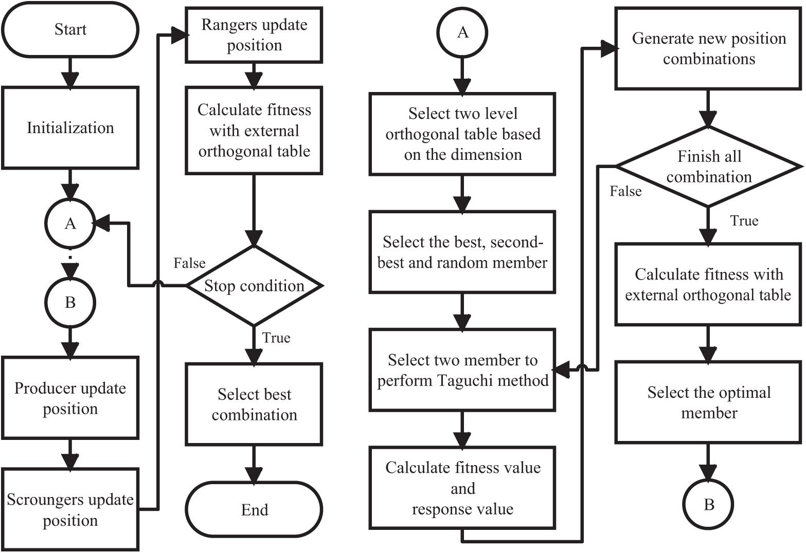
Figure 2: The flowchart of AT-GSO algorithm

Here is the process description of the AT-GSO algorithm. A parameter Xp is introduced to denote the number of producers, with a recommended range of Xp ∈ [1, 10] in the initial setup of the AT-GSO algorithm. The AT-GSO algorithm selects the individuals with the highest two fitness scores as producers in each iteration, known as Xp1 and Xp2, respectively. The remaining group members select a third producer, Xp3, to ensure diversity. The factor levels in the orthogonal experimental design are set by these three producers. As a result, three crossover types are chosen. Xp1 and Xp2 are assigned as the first and second levels in each iteration, along with combinations of Xp1, Xp2, and Xp3. An orthogonal table Lm(2m−1) is selected, and three experiments are conducted for different level combinations of Xp. Where m denotes the number of rows of the orthogonal experiment; m – 1 denotes the number of columns of configurable decision parameters. Three new producers are generated after completing the Taguchi Method, Xnp1, Xnp2 and Xnp3, respectively. These new producers identify the optimal producer Xop for each iteration, enhancing both the robustness of the search process and the efficiency in locating global optima.

The tolerance design optimization problem is described as follows:

Minimize{f(x)|x∈[l,u]},subject to the design constraints and the tolerance Δx of x,(9)

where f(x) is the object function, x=(x1,x2,…,xn)∈Rn is a set of vectors with n variables in the nominal value of the design, Δx is the tolerance of x, l, and u is the solution space of x.

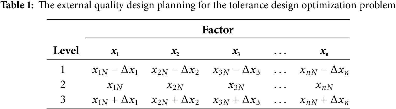
The orthogonal table of three levels Lm(3(m−1)/2) is used to build the external quality design planning to solve the tolerance design optimization problem, as shown in Table 1.

The design nominal and tolerance values should be considered in practical design scenarios. This means that while achieving the optimal target value, the tolerances resulting from parameter variations can also be reduced. Thus, Eq. (9) is re-described as follows:

Minimize {μ(f(x±Δx))andσ(f(x±Δx))}, subject to the design constraints(10)

where μ(f(x±Δx)) is the average value of f(x±Δx) in the tolerance experiment and σ(f(x±Δx)) is the standard deviation of f(x±Δx) in the tolerance experiment.

The evolutionary algorithms assess and solve the problem based on fitness values rather than objective function values due to variations in component specifications in the optimization problems. The objective function method solely accounts for system performance f(x) but neglects the effect of allowable error △x of the design parameter x on system performance. However, the influence of the allowable error △x in the design parameter x on system performance can be considered alongside the system’s performance by applying the fitness function approach. Thus, choosing and designing system parameters using an adaptive function minimizes the sensitivity of the desired target value to changes in the specifications of specific uncontrollable components. For the optimization problem where smaller values are preferred, Eq. (10) can be expressed using the fitness function as follows:

F=μ(f(x±Δx))+wσ(f(x±Δx)),(11)

where w is the weight factor to balance between μ(f(x±Δx)) and σ(f(x±Δx)).

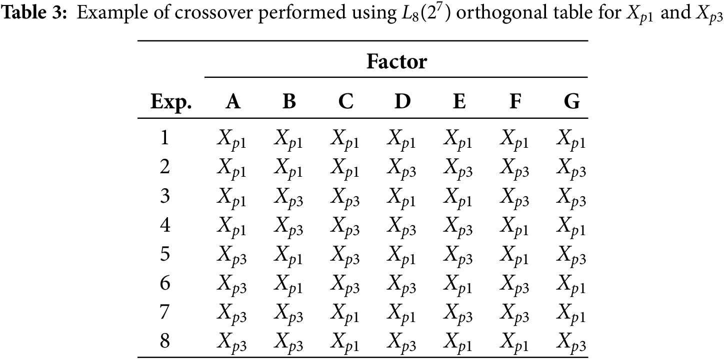
For example, suppose each producer has seven dimensions and two levels. The orthogonal table L8(27) is employed, as shown in Tables 2–4. The experiment is repeated three times for each row combination of the orthogonal experiment. After the orthogonal experiment is completed, three results are obtained for each row combination. Eq. (12) identifies which level had a more significant influence on each factor and ensures robustness in the search for the optimal value.

Efj=−10⋅log((Ji(avg)2/JMax,avg2)+(Ji(std)2/JMax,std2)), j=1,2,(12)

where Ji(avg) is the average of the three results; Ji(std) is the standard deviation of the three results; JMax,avg is the maximum average in the orthogonal experiment; JMax,std is the maximum standard deviation in the orthogonal experiment.

After selecting the optimal level for all factors, a new producer vector Xnpi (i = 1, 2, 3) is generated. In the end, six producer vectors Xp1, Xp2, Xp3, Xnp1, Xnp2 and Xnp3 are acquired, and their fitness values are calculated with external orthogonal table separately. The producer with the highest fitness is selected as the optimal producer Xop for the current iteration. Next, the original GSO algorithm update position process is executed.

2.3 Tolerance Design of Heat Exchanger System

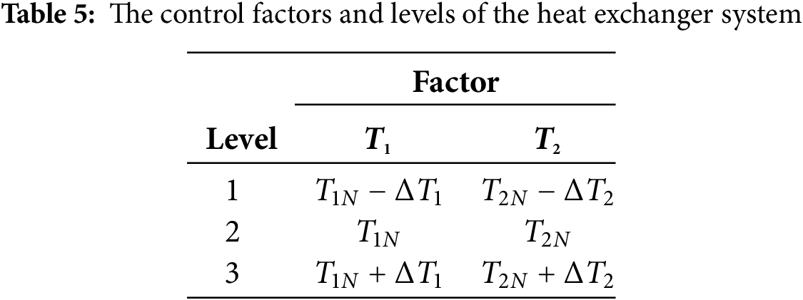
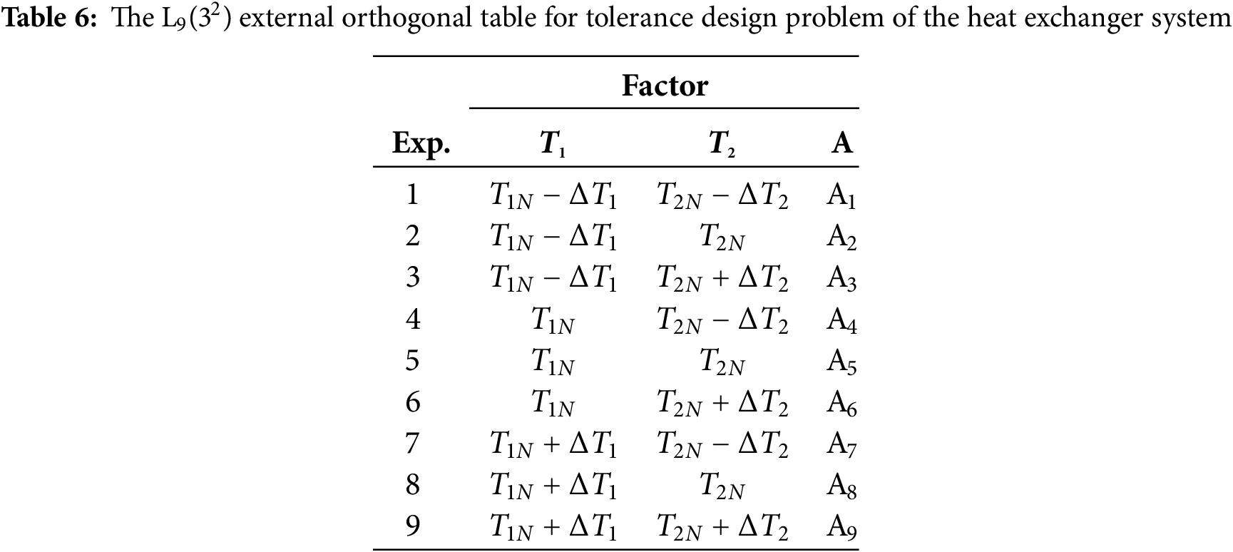
Fixing a system’s operating temperature at a constant state is difficult, and there is bound to be an uncertainty error in industry applications [17]. It is straightforward to find the optimal parameters without tolerance in a robust heat exchanger system, but considering tolerance tends to reduce the robustness of the system. This paper uses three tolerance values: ±10%, ±20% and ±40%. Since the heat exchanger system has two operator temperature parameters, the L9(32) external orthogonal table simulates the tolerance design problem. The two parameters of the heat exchanger system are defined as follows:

T=[T1,T2].(13)

The two parameters and tolerance levels of the heat exchanger system are shown in Table 5; the external orthogonal table is shown in Table 6. All two parameters must satisfy the following equation:

T={100≤T1≤300 and  T1≤T2≤400}.(14)

3  Results and Discussions

This paper uses Eq. (2) to evaluate the performance of the heat exchanger system by the AT-GSO algorithm. Two types of experiments: heat exchanger system without tolerance and heat exchanger system with tolerance. Five independent experiments will be conducted on the hyperparameters of the AT-GSO algorithm. Since the heat exchanger system has two parameters, the dimension of the AT-GSO algorithm is 2, the search range of each dimension is [100, 400], the population size is 10, and the maximum iteration is 50. This paper evaluates the proposed algorithm’s performance by comparing it with the fractional-order particle swarm optimization (FPSO) [19].

3.1 Experimental Results of AT-GSO for Designing of Heat Exchanger System

The AT-GSO hyperparameters are set as follows: the number of producers is 3, the percentage of rangers is 60%, the maximum search angle (θmax) of producer is π/α2 × 1.8, the maximum turning angle (αmax) of producer is θmax/4, the longest search distance of producer is 8, and the initial angle is π/2. Five independent experiments without tolerance will be conducted using this combination of AT-GSO hyperparameters and the results are shown in Table 7. The average A-value (the total heat transfer area) is 7049.2502; the standard deviation A-value is 1.71 × 10−3. The results of the five FPSO independent experiments without tolerance are presented in Table 8. Fig. 3 shows the mean fitness value curves for the AT-GSO and FPSO algorithms, each averaged over five experiments. Both the AT-GSO and FPSO algorithms can find the optimal value without tolerance. However, as shown in Fig. 3, FPSO exhibits significant instability during the search process. Furthermore, Tables 7 and 8 demonstrate that AT-GSO outperforms FPSO and exhibits greater robustness.

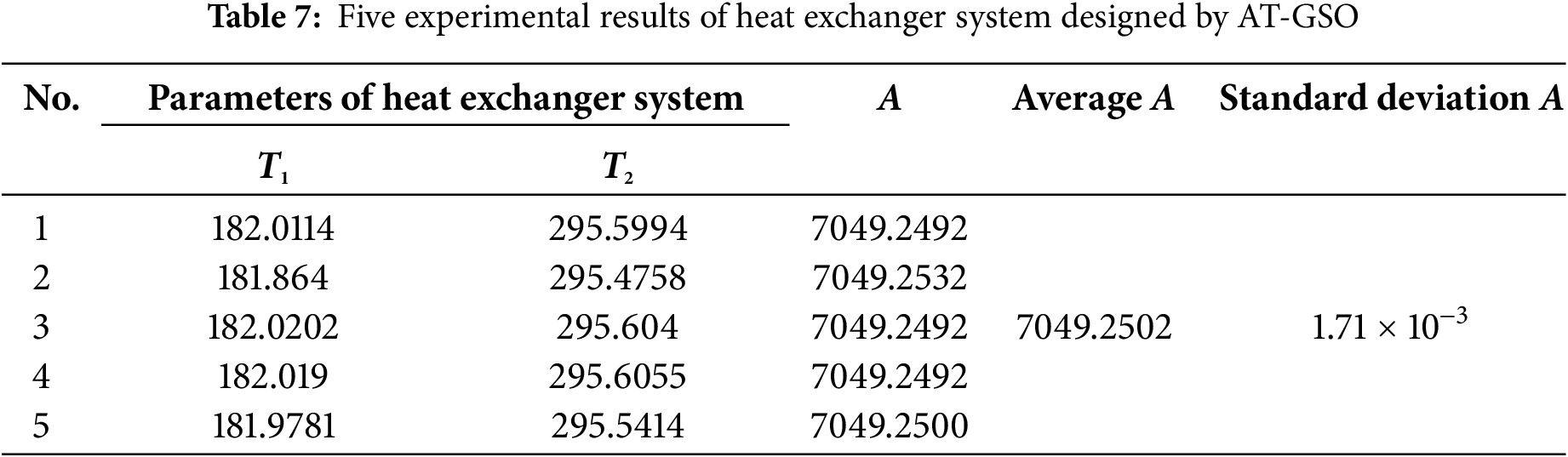
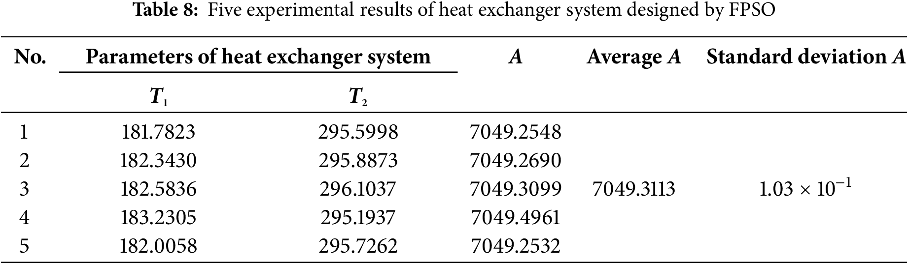
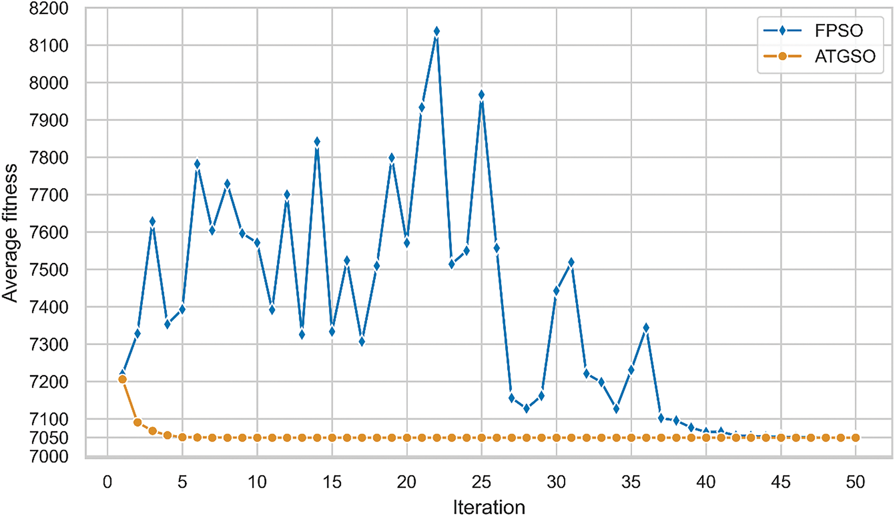
Figure 3: The fitness curve of five experiments of heat exchanger system without tolerance designed by AT-GSO

3.2 Experimental Results of AT-GSO for Tolerance Design of Heat Exchanger System

This paper uses three tolerance values: ±10%, ±20% and ±40%. The AT-GSO hyperparameters with ±10% tolerance are set as follows: the number of producers is 3, the percentage of rangers is 60%, the maximum search angle (θmax) of producer is π/α2 × 1.8, the maximum turning angle (αmax) of producer is θmax/4, the longest search distance of producer is 8, and the initial angle is π/2. Five independent experiments with ±10% tolerance will be conducted using this combination of AT-GSO hyperparameters and the results are shown in Table 9. The average A-value (the total heat transfer area) is 7049.2502; the standard deviation A-value is 1.71 × 10−3. The results of the five FPSO independent experiments are presented in Table 10. Fig. 4 shows the mean fitness value curves for the AT-GSO and FPSO algorithms, each averaged over five experiments. Both the AT-GSO and FPSO algorithms can find the optimal value with ±10% tolerance. However, as shown in Fig. 4, FPSO exhibits instability during the search process. Furthermore, Tables 9 and 10 demonstrate that AT-GSO outperforms FPSO and exhibits greater robustness.

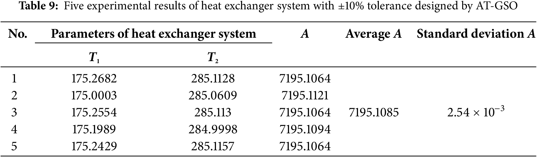
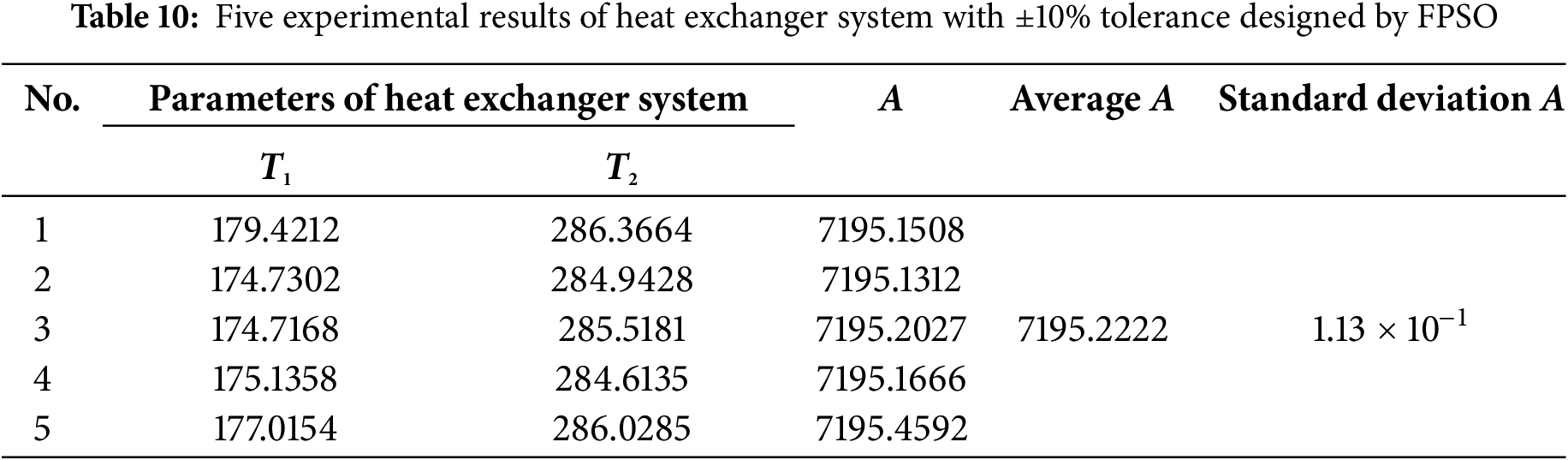
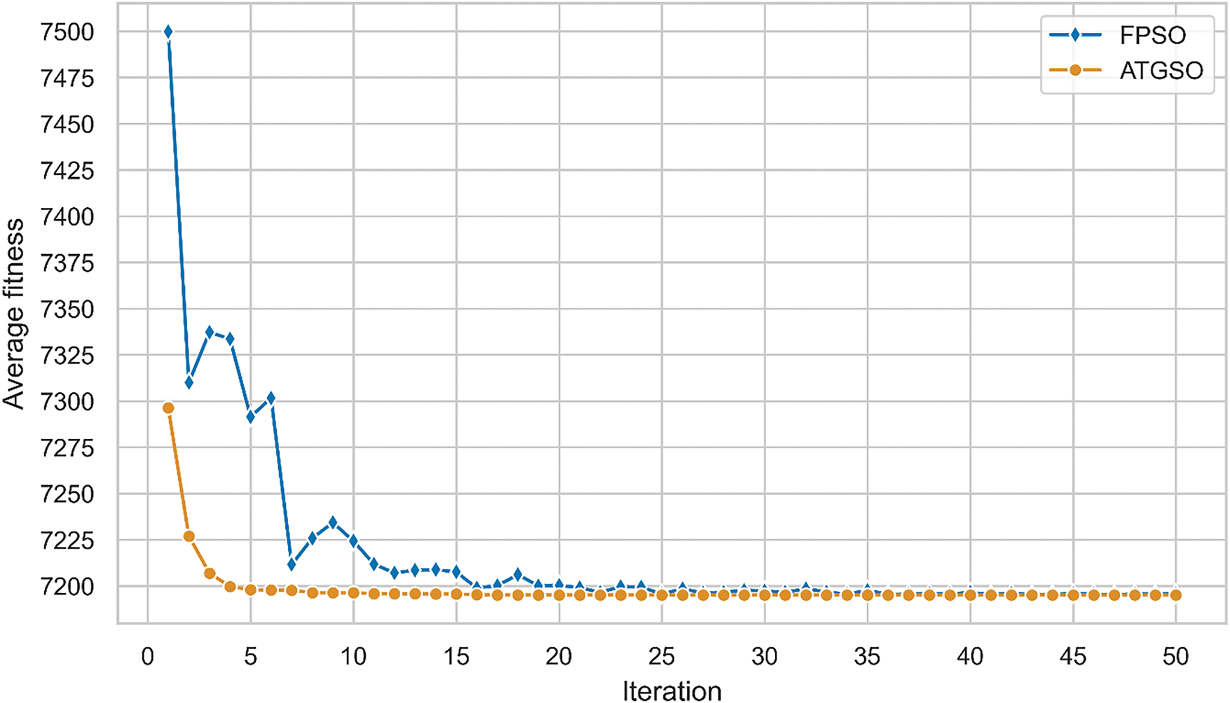
Figure 4: The fitness curve of five experiments of heat exchanger system with ±10% tolerance designed by AT-GSO

The AT-GSO hyperparameters with ±20% tolerance are set as follows: the number of producers is 10, the percentage of rangers is 90%, the maximum search angle (θmax) of producer is π/α2 × 1.6, the maximum turning angle (αmax) of producer is θmax/6, the longest search distance of producer is 2, and the initial angle is π/3. Five independent experiments with ±20% tolerance will be conducted using this combination of AT-GSO hyperparameters and the results are shown in Table 11. From Table 11, it is learnt that AT-GSO did not search for the best parameter in one out of five experiments. The average A-value (the total heat transfer area) is 7380.1461; the standard deviation A-value is 7.69 × 10−1. The results of the five FPSO independent experiments are presented in Table 12. Fig. 5 shows the mean fitness value curves for the AT-GSO and FPSO algorithms, each averaged over five experiments. Table 12 shows that the FPSO algorithms fail to find the optimal value with ±20% tolerance, falling into a local optimum solution. As shown in Fig. 4, FPSO exhibits instability during the search process. Furthermore, Tables 11 and 12 demonstrate that AT-GSO outperforms FPSO.

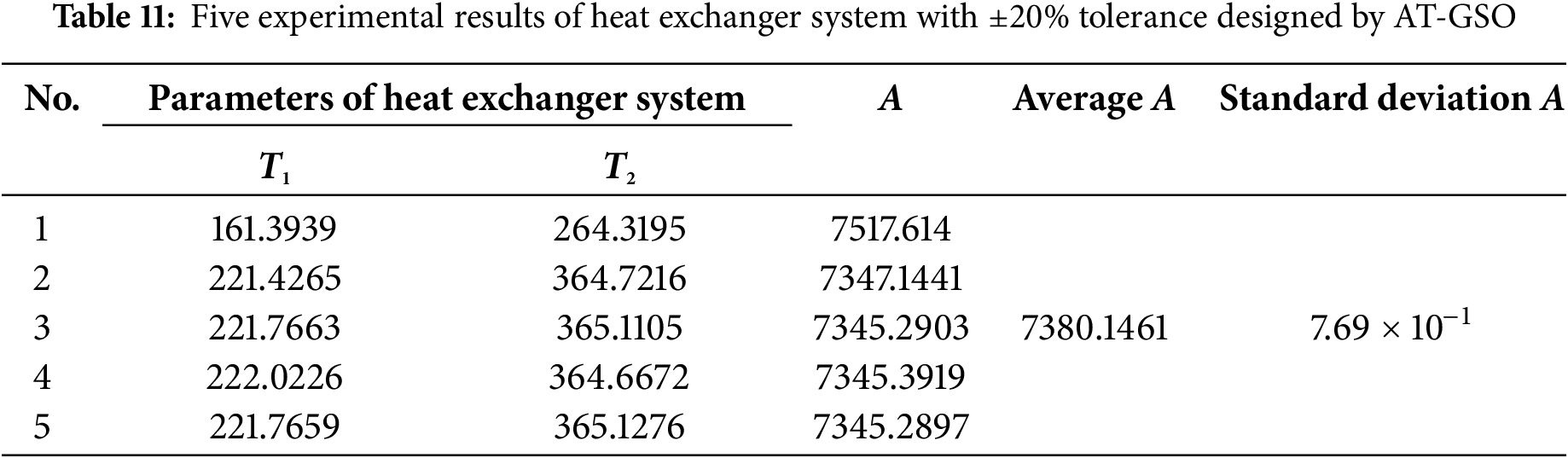
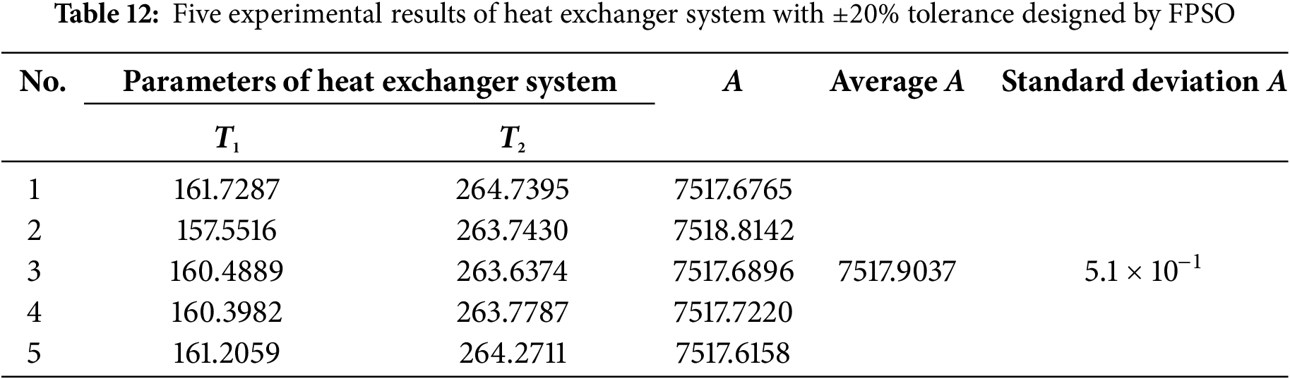
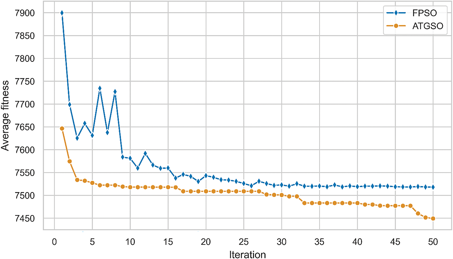
Figure 5: The fitness curve of five experiments of heat exchanger system with ±20% tolerance designed by AT-GSO

The AT-GSO hyperparameters with ±40% tolerance are set as follows: the number of producers is 3, the percentage of rangers is 60%, the maximum search angle (θmax) of producer is π/α2 × 1.8, the maximum turning angle (αmax) of producer is θmax/4, the longest search distance of producer is 8, and the initial angle is π/2. Five independent experiments with ±40% tolerance will be conducted using this combination of AT-GSO hyperparameters and the results are shown in Table 13. The average A-value (the total heat transfer area) is 7049.2502; the standard deviation A-value is 1.71 × 10−3. The results of the five FPSO independent experiments with ±40% tolerance are presented in Table 14. Fig. 3 shows the mean fitness value curves for the AT-GSO and FPSO algorithms, each averaged over five experiments. Both the AT-GSO and FPSO algorithms can find the optimal value without tolerance. However, as shown in Fig. 6, FPSO exhibits significant instability during the search process. Furthermore, Tables 13 and 14 demonstrate that AT-GSO outperforms FPSO and exhibits greater robustness.

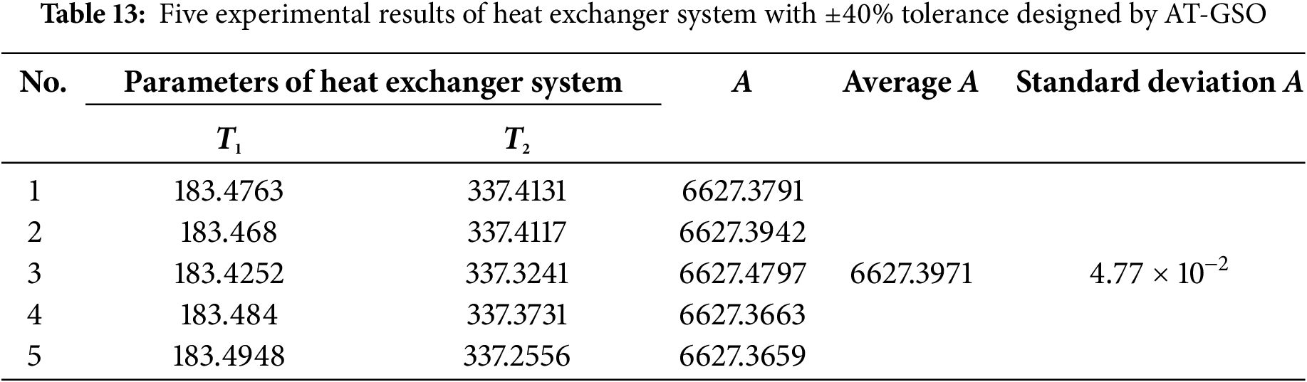
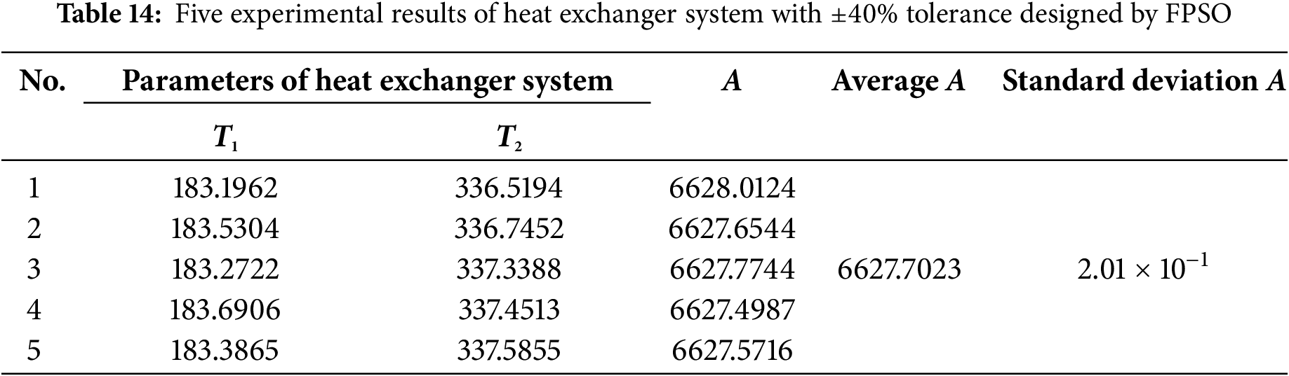
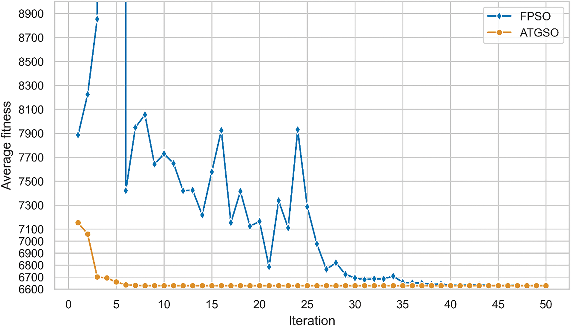
Figure 6: The fitness curve of five experiments of heat exchanger system with ±40% tolerance designed by AT-GSO

4  Conclusions

This paper proposed the AT-GSO algorithm, which combines the R-GSO algorithm and external quality design planning of the Taguchi method to optimize the heat exchanger system to minimize the total heat transfer area. The AT-GSO algorithm has a tolerance design capability. In the industry, keeping the operating temperature of a heat exchanger system in a constant state is not easy. This paper allows three tolerance values for operating temperature: ±10%, ±20% and ±40%. Experimental outcomes indicate that the AT-GSO algorithm proficiently optimizes the heat exchanger system and finds the optimum operating temperature without and with all three tolerances. The method proposed in this paper can take into account the existence of uncertainties in the parameters during the parameter optimization process so that it can reduce the impact caused by the errors in the parameters in practical applications. In future work, the method proposed in this paper can be applied to different algorithms and different applications. While tolerances were introduced for operating temperatures, other potential uncertainties (e.g., flow rate variations, fluid properties, or fouling factors) were not considered. In addition, this paper currently minimizes only the total heat transfer area, while other objectives are not included in the optimization process.

Acknowledgement: The authors thank the National Science and Technology Council, Taiwan for supporting this work.

Funding Statement: Publication costs are funded by the National Science and Technology Council, Taiwan, under Grant Number MOST110-2221-E035-092-MY3.

Author Contributions: The authors confirm contribution to the paper as follows: study conception and design: Yu-Cheng Liao and Jyh-Horng Chou; data collection and programming: Yu-Cheng Liao; analysis and interpretation of results: Yu-Cheng Liao and Fu-I Chou; draft manuscript preparation: Yu-Cheng Liao, Fu-I Chou and Po-Yuan Yang. All authors reviewed the results and approved the final version of the manuscript.

Availability of Data and Materials: All data generated or analyzed during this study are included in this published article.

Ethics Approval: Not applicable.

Conflicts of Interest: The authors declare no conflicts of interest to report regarding the present study.

References

1. Roy R. Taguchi method. New York, NY, USA: Van Nostran Reinhold; 1990. [Google Scholar]

2. Celik N, Pusat G, Turgut E. Application of Taguchi method and grey relational analysis on a turbulated heat exchanger. Int J Therm Sci. 2018;124(1):85–97. doi:10.1016/j.ijthermalsci.2017.10.007. [Google Scholar] [CrossRef]

3. Raei B. Statistical analysis of nanofluid heat transfer in a heat exchanger using Taguchi method. J Heat Mass Transf Res. 2021;8(1):29–38. doi:10.22075/jhmtr.2020.20678.1287. [Google Scholar] [CrossRef]

4. Xie X, Tang S, Zhou J, Zhang D, An J, Wu X. Parametric study and optimization of H-type finned tube heat exchangers with honeycomb arrangement using Taguchi method. Appl Therm Eng. 2024;256(10):124116. doi:10.1016/j.applthermaleng.2024.124116. [Google Scholar] [CrossRef]

5. Zhang T, Chen L, Wang J. Multi-objective optimization of elliptical tube fin heat exchangers based on neural networks and genetic algorithm. Energy. 2023;269(1):126729. doi:10.1016/j.energy.2023.126729. [Google Scholar] [CrossRef]

6. Balaji C, Srinivasan B, Gedupudi S. Heat transfer engineering: fundamentals and techniques. Cambridge, MA, USA: Academic Press; 2020. [Google Scholar]

7. Shahin K. Heat exchanger design and optimization. In: Laura Castro G, Víctor Manuel Velázquez F, Miriam Navarrete P, editors. Heat exchangers. Rijeka, Croatia: IntechOpen; 2021. [Google Scholar]

8. Venkatesh B, Kiran A, Khan M, Rahmani MKI, Upadhyay L, Babu JC, et al. Performance optimization for an optimal operating condition for a shell and heat exchanger using a multi-objective genetic algorithm approach. PLoS One. 2024;19(6):e0304097. doi:10.1371/journal.pone.0304097. [Google Scholar] [PubMed] [CrossRef]

9. Bianco N, Fragnito A, Iasiello M, Mauro GM, Mongibello L. Multi-objective optimization of a phase change material-based shell-and-tube heat exchanger for cold thermal energy storage: experiments and numerical modeling. Appl Therm Eng. 2022;215(11):119047. doi:10.1016/j.applthermaleng.2022.119047. [Google Scholar] [CrossRef]

10. Yang X, Zhao W, Cheng X, Dong W, Luo W, Zhao Q. Experimental and numerical optimization study on an airfoil-shaped heat exchanger. Proc Inst Mech Eng Part A J Power Energy. 2023;237(7):1526–38. doi:10.1177/09576509231169545. [Google Scholar] [CrossRef]

11. Rani P, Barmavatu P. Numerical investigations and design optimization of cryogenic plate-fin heat exchanger in Electric Arc Furnace using radiative heat transfer model. Numer Heat Transf Part B Fundam. 2024;2024:1–22. doi:10.1080/10407790.2024.2331804. [Google Scholar] [CrossRef]

12. Gawai IR, Lalwani DI. Optimization of three-stage heat exchanger design using modified differential evolution algorithm. In: Scientific and technological advances in materials for energy storage and conversions. Singapore: Springer Nature Singapore; 2024. p. 1–13. doi:10.1007/978-981-97-2481-9_1. [Google Scholar] [CrossRef]

13. Bakr M, Hegazi AA, Haikal AY, Elhosseini MA. Genetic algorithm for the design and optimization of a shell and tube heat exchanger from a performance point of view. Int J Electr Comput Eng Syst. 2022;13(7):601–10. doi:10.32985/ijeces.13.7.12. [Google Scholar] [CrossRef]

14. Zhang Y, Wei Z, Zhang Y, Wang X. Inverse problem and variation method to optimize cascade heat exchange network in central heating system. J Therm Sci. 2017;26(6):545–51. doi:10.1007/s11630-017-0972-1. [Google Scholar] [CrossRef]

15. Shafiey Dehaj M, Hajabdollahi H. Fin and tube heat exchanger: constructal thermo-economic optimization. Int J Heat Mass Transf. 2021;173(4):121257. doi:10.1016/j.ijheatmasstransfer.2021.121257. [Google Scholar] [CrossRef]

16. Wu J, Liu S, Wang M. Process calculation method and optimization of the spiral-wound heat exchanger with bilateral phase change. Appl Therm Eng. 2018;134(1):360–8. doi:10.1016/j.applthermaleng.2018.01.128. [Google Scholar] [CrossRef]

17. Xue Y, Yang H. A numerical method to estimate temperature intervals for transient convection-diffusion heat transfer problems. Int Commun Heat Mass Transf. 2013;47(6):56–61. doi:10.1016/j.icheatmasstransfer.2013.07.005. [Google Scholar] [CrossRef]

18. Deng ZL. Optimization methods in the chemical industry. Beijing, China: Chemical Industry Press; 1992. [Google Scholar]

19. Cheng Y-C. Optimal Design of H2/H∞ PIMD controller by using fractional-order particle swarm optimizer [master’s thesis]. Kaohsiung, Taiwan: National Kaohsiung University of Science and Technology; 2020. [Google Scholar]