Improving Shallow Foundation Settlement Prediction through Intelligent Optimization Techniques

1  Introduction

The interface where the structure connects with the ground is referred to as the foundation. Shallow foundations are critical in transferring the load of the pavement to the underlying soil. After construction, the foundation is subjected to both gravity and live loads originating from the pavement [1,2]. Many situations involve shallow foundations experiencing cyclic loads along with static loads, including those caused by earthquake forces, traffic, and machinery-induced vibrations [3,4]. These loads generally induce secondary stresses in shallow foundations, resulting in increased settlement (Sm) and, in some cases, the potential for foundation failure [5–7]. The anticipation and assessment of Sm stands as a paramount and complex quandary that confronts geotechnical engineers. The quantum of foundation subsidence is contingent upon a myriad of variables, encompassing factors such as foundation dimensions, soil composition, applied load magnitude, load type, foundation, and pavement solidity. Extensive research endeavors have been undertaken to investigate foundation settlement utilizing conventional methodologies and established correlations. For instance, Kusakabe [8] investigated the effect of footing size on the shape factor Sγ using centrifuge experiments and analytical predictions. They revealed that as the footing size increased from several centimeters to 3 m, the shape factor Sγ decreased by 33%. This demonstrates the significant impact of footing size on foundation behavior. Khing et al. [9], employing a tangible model within a laboratory setting, explored the load-bearing capacity and settlement magnitude of rigid strip foundations embedded in sandy soil. Their findings revealed that the zenith of foundation subsidence typically materializes at approximately 10% of the strip foundation’s width. Shahir et al. [10] ventured to predict foundation settlement by harnessing numerical techniques. They conducted a centrifuge experiment and then subjected it to a comparison against empirical measurements to validate their numerical framework. Foye et al. [11] adeptly deployed finite element methods to gauge Sm in the context of square, rectangular, and strip foundations on clayey terrains. Eid [12] employed numerical analysis to explore the behavior of shallow foundations on sandy substrates. They conducted a miniature-scale physical model test to substantiate and enhance the precision of their numerical analysis. They ultimately utilized the insights gleaned from their analysis-driven graphs and equations to derive Sm estimates. Kim et al. [13] conducted a comprehensive exploration of the impact of rainfall on foundation settlement through numerical analysis. Then, they juxtaposed these numerical findings against field measurements, revealing a substantial alignment between the load-settlement relationships obtained from numerical and field methods. These outcomes highlighted the influence of rainfall intensity on Sm within unsaturated soils. In a similar vein, Cong et al. [14] investigated the differential seismic Sm under varying load conditions using finite element software. Their deductions revealed that higher load magnitudes lead to excessive settlement, with the ratio of length to width emerging as a significant factor influencing the extent of differential seismic Sm. Utilizing numerical modeling, Hakro et al. [15] determined the applied loadings on foundations and gauged saturation levels. Their findings illuminated that the degree of saturation holds greater sensitivity to foundation settlement than the degree of loading. Tabaroei et al. [16] in a laboratory setting, delved into the behavior of circular footings in sandy soil. They elucidated their results through load-settlement diagrams and the spatial distribution of pressure across specific foundation points. Their research divulged that an increase in distance from the foundation center correlates with a reduction in both vertical pressure and settlement magnitude. In a different context, Tasiopoulou et al. [17] created a model to predict foundation settlement in sandy substrates using FLAC 2D and 3D software. Their model’s outputs were benchmarked against experimental methods, leading to the conclusion that the extent of foundation settlement closely aligns across the two cases. Zhu et al. [18] conducted a detailed study on the scale effect of strip and circular footings on bearing capacity by employing both numerical simulations and experimental analysis. Their results revealed an exponential increase in bearing capacity as the footing dimensions grow larger. Therefore, this leads to a decrease in the bearing capacity factor Nγ with increasing footing size. In their research, they also explored the bearing capacity and settlement behavior of shallow circular foundations, utilizing a nonlinear constitutive relationship and performing simulations using Abaqus software [19]. This approach allowed them to more accurately model the complex interactions between soil and foundation, providing deeper insights into the effect of footing size on performance.

Although the studies conducted provide substantial value, it becomes evident that traditional approaches in the mentioned research fail to account for uncertainties and variations in geological parameter values, thus compromising their accuracy. In addition, specific techniques, such as regression methods, are limited in addressing nonlinearity and complex equations. Laboratory and field-based methods can also introduce errors due to testing frequency at specific points, leading to time and cost inefficiencies as well as potential inaccuracies from fatigue. These limitations highlight the need for methodologies capable of handling uncertainties in geotechnical parameters, efficiently generating nonlinear and complex equations, and encompassing the full range of parameters influencing model outcomes in a cost-effective and timely manner [20]. As a result, an increasing number of researchers and engineers are turning to soft computing methods and algorithms for predicting and estimating Sm, recognizing their ability to accommodate input parameter variability, complex geotechnical considerations, nonlinear modeling, and the dynamic interaction between soil and foundations. Thus, modern intelligent methodologies have emerged as powerful tools for accurate Sm estimation, providing a closer alignment with real-world scenarios.

Several studies have addressed this topic. For example, Shahin et al. [21] predicted the settlement of shallow foundations on cohesionless soils using artificial neural networks (ANN). Samui [22] applied support vector machines (SVM), a novel learning algorithm based on statistical theory, to predict shallow foundation settlement on cohesionless soil. Soleimanbeigi et al. [23] used a feedforward backpropagation neural network (BPNN) to predict the settlement of reinforced foundations. The model performed well, demonstrating its potential as an accurate tool for predicting shallow reinforced foundation settlements on cohesionless soils. Shahin et al. [24] employed backpropagation neural networks to predict settlement in shallow foundations on cohesionless soils. Gnananandarao et al. [25] employed feedforward neural networks with backpropagation algorithms to predict shallow foundation settlement on granular soils, revealing that foundation width had the greatest impact on settlement predictions. Luat et al. [26] proposed a hybrid artificial intelligence model, Genetic Algorithm Integrated with Multivariate Adaptive Regression Splines (GA-MARS), to predict settlement in shallow foundations on sandy soils. They showed that the GA-MARS model outperformed existing methods. Shahin et al. [27] utilized B-spline networks, a type of neural network, to predict shallow foundation settlement. These networks were trained using the Adaptive Spline Modeling of Observational Data (ASMOD) algorithm, which improved model accuracy and interpretability by incorporating existing engineering knowledge. Mohammed et al. [28] emphasized the use of the Adaptive Neuro-Fuzzy Inference System (ANFIS) combined with Particle Swarm Optimization (PSO), Differential Evolution (DE), Ant Colony Optimization (ACO), and Genetic Algorithm (GA) for analyzing shallow foundation settlements. Their results showed that the ANFIS-PSO model provided the most accurate and reliable predictions. Shahin et al. [29] successfully utilized artificial neural networks (ANN) to solve the complex problem of estimating settlement in shallow foundations on granular soils, which had previously been addressed with low accuracy by traditional methods. Wan [30] explored the use of machine learning methods, such as hybrid support vector regression (SVR) combined with sine-cosine algorithms (SCA) and bat-inspired algorithms (BAT), to identify shallow foundation settlements. The SCA-SVR method outperformed BAT-SVR and ANFIS-PSO in terms of classification accuracy. Krishna Pradeep et al. [31] employed a combined PSO-ANN technique to predict settlement in shallow foundations on cohesionless soils. Tsai et al. [32] proposed a genetic programming system (GPS), including genetic programming (GP), weighted genetic programming (WGP), and soft computational polynomials (SCP), to determine the ultimate bearing capacity of shallow foundations. Their results demonstrated that all GPS models outperformed other methods in terms of prediction accuracy. Finally, Ray et al. [33] investigated the use of three soft computing techniques, minimum likelihood machine regression (MLMR), ANN based on PSO, and adaptive neuro-fuzzy inference system based on PSO (ANFIS-PSO), for shallow foundation prediction. Their analysis showed that the MLMR model performed better than the other methods.

In light of the explanations and research provided, methods capable of accurately accounting for uncertainties in input parameters should be employed. This study aims to explore algorithms that have not been previously addressed to demonstrate the efficiency of these methods. Specifically, two intelligent algorithms, Teaching-Learning-Based Optimization (TLBO) and Harmony Search (HS), are utilized to establish a relationship and model for the Sm. Given their fine-tuning parameters and ease of implementation, these algorithms are expected to exhibit superior accuracy compared to other intelligent methods discussed in the previous studies. The validation and evaluation of the developed model are conducted using statistical criteria, including the mean square error (MSE), coefficient of determination (R2), and root mean square error (RMSE). The results conclusively show that the use of HS and TLBO algorithms represents a robust and effective approach for estimating Sm.

2  Data Collection

It is imperative to examine soil characteristics meticulously to achieve a highly accurate and dependable assessment of soil compressibility at foundation depth. Therefore, the Standard Penetration Test (SPT) emerges as a frequently employed technique to deduce and quantify compressibility in non-cohesive soils. Despite being associated with expenses, time consumption, and some level of imprecision, SPT examinations continue to find widespread use on a global scale. An integral aspect of the SPT test involves the computation of the standard penetration number, a parameter of significant importance [34–37]. The standard penetration number is influenced by various factors, often necessitating adjustments through the relationship depicted below:

N70′=N×CN×η1×η2×η3×η4...(1)

where N70′ is the standardized penetration value adjusted to encompass 70% of the hammer’s impact energy, N represents the computed standard penetration number, CN is the ratio of the overburden pressure, η1 is the impact energy coefficient on average, η2 is the coefficient linked to the length of the drilling rod, η3 pertains to the coefficient related to sample conditions, and η4 is the coefficient associated with borehole diameter. Although Burland et al. [38] proposed that neither overburden pressure nor submergence corrections are necessary for N, Terzaghi et al. [39] suggested modifying the N value if it is recorded underwater or in the presence of water within muddy or fine sands.

N′=15+0.5(N−15)(2)

In the case of gravel or sand, the penetration number N is adjusted as indicated below:

N′=1.25N(3)

Although the SPT test and the number of blows provide useful insights into soil characteristics and permeability, they alone are insufficient for providing a complete or highly accurate estimate of foundation settlement. It is critical to identify and understand the various factors that significantly influence this parameter to achieve more precise predictions of Sm (settlement in millimeters). The key contributors to the model’s output include the width of the footing (B), the pressure exerted on the footing (q0), the count of SPT blows (N), the ratio of footing embedment (Df/B), and the geometry of the footing (L/B). These parameters all play a significant role in determining the settlement behavior, with each having a varying degree of impact on the model’s outcome. Fig. 1 provides a schematic representation of how these parameters collectively influence Sm. In addition, based on the illustration in Fig. 1, it can be more accurate to refer to q0, as this more specifically characterizes the parameter within the context of the study. More reliable and accurate models for predicting foundation settlement can be developed by understanding how these variables interact and contribute to the final result.

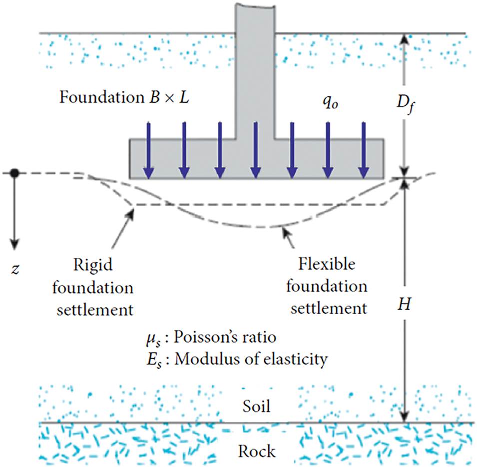
Figure 1: Illustration of Parameters Affecting Shallow Foundations, where q0 represents the pressure exerted on the footing [28]

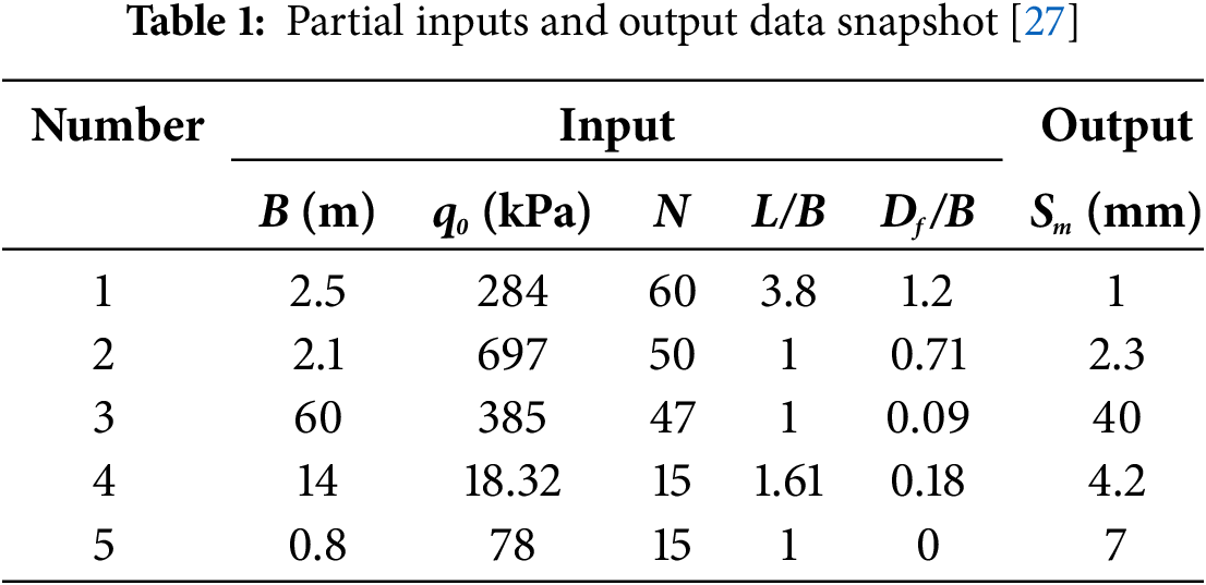
Considering the inherent variability in both input and output parameters (attributed to uncertainty), this study harnessed a dataset comprising 189 data points. Hence, Table 1 lists a subset of the measured input and output data values essential for model construction [40].

It is essential in data mining analysis to examine statistical information such as data dispersion, outlier data, data distribution, central tendency, and the overall data pattern to ensure a more accurate model analysis. The box plot is a standard method for displaying data using statistical indicators: “minimum value”, “first quartile-Q1”, “median”, “third quartile-Q3”, and “maximum value”, as presented in Table 2 and Fig. 2. Based on Fig. 2 and Table 2, greater distances between the maximum and minimum values and the length of the box indicate higher data dispersion. Therefore, Fig. 2 indicates a greater data dispersion in the upper part of the data range. In addition, statistical information helps identify outliers. It reveals that the absence of data points above or below the box plot indicates no outliers in the data. Outliers, if present, can lead to low-accuracy modeling and should be excluded. Hence, in the current modeling, no data points were removed, and all data were utilized.

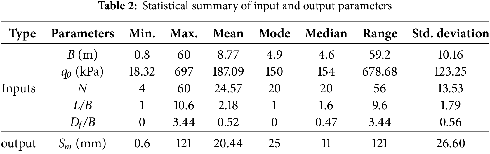
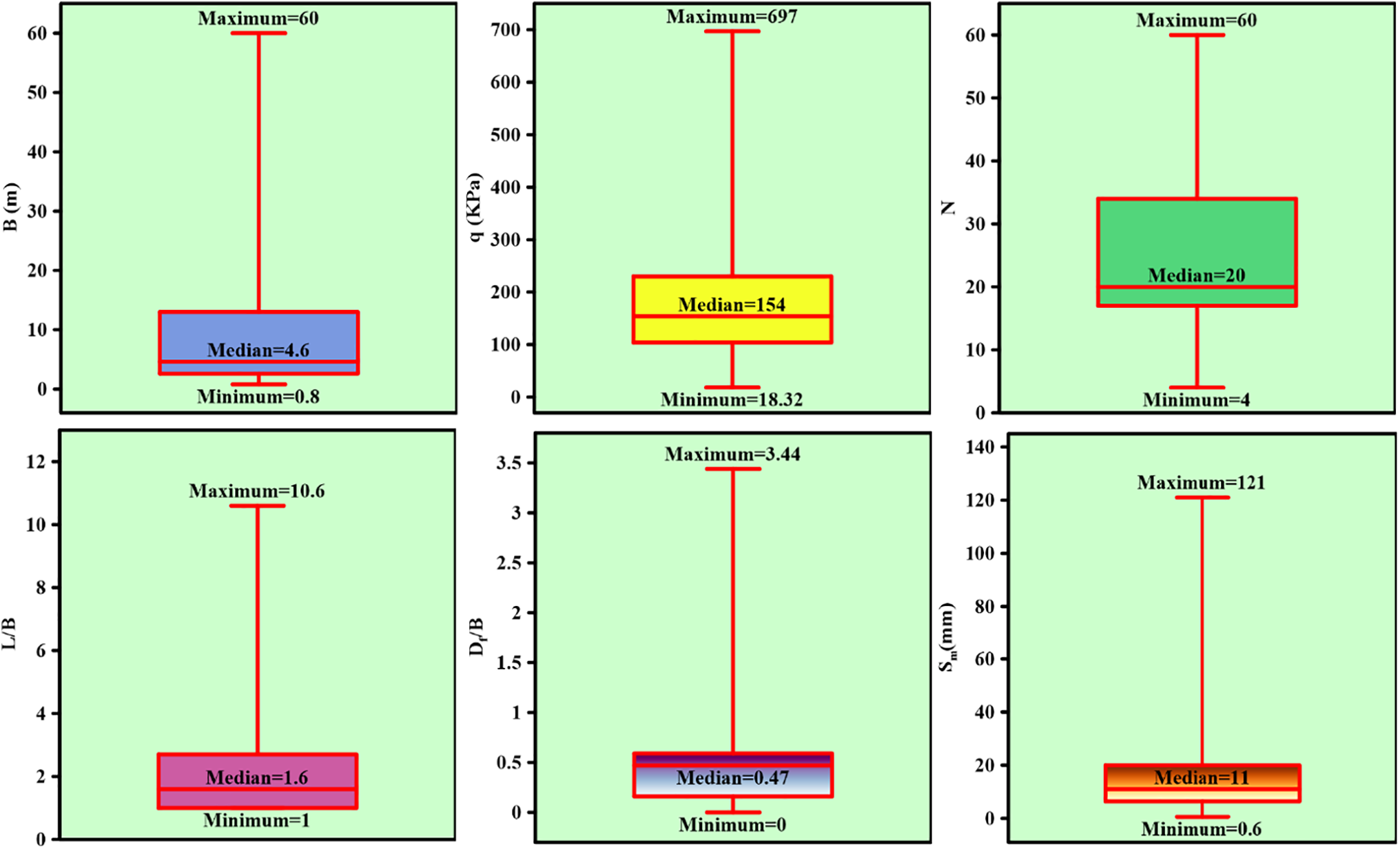
Figure 2: Box plot representing input and output parameters

In addition, the median of the parameters q0 (kPa) and L/B lies approximately in the middle of the box length, indicating a normal distribution, while the other parameters exhibit right or left skewness. Table 2 also shows that the parameters Df/B and L/B are clustered around the mean and are not significantly deviated from it.

3  Overview of Methodologies

Over the past forty years, numerous algorithms have emerged for the resolution of engineering optimization challenges. These approaches present a significantly improved alternative to conventional methods, showing the capability to accurately depict complex and nonlinear issues. This research explores the utilization of two distinct algorithmic frameworks to forecast Sm, both of which are elaborated upon in the subsequent sections.

3.1 Harmony Search Algorithm (HS)

The HS algorithm, introduced by Geem et al. in 2001, is inspired by the harmonious interplay in music creation. It mimics musicians crafting harmonious compositions to find optimal solutions to optimization problems [41,42]. Fig. 3 illustrates the HS algorithm’s operation, depicting its pursuit of harmonious and melodious outcomes.

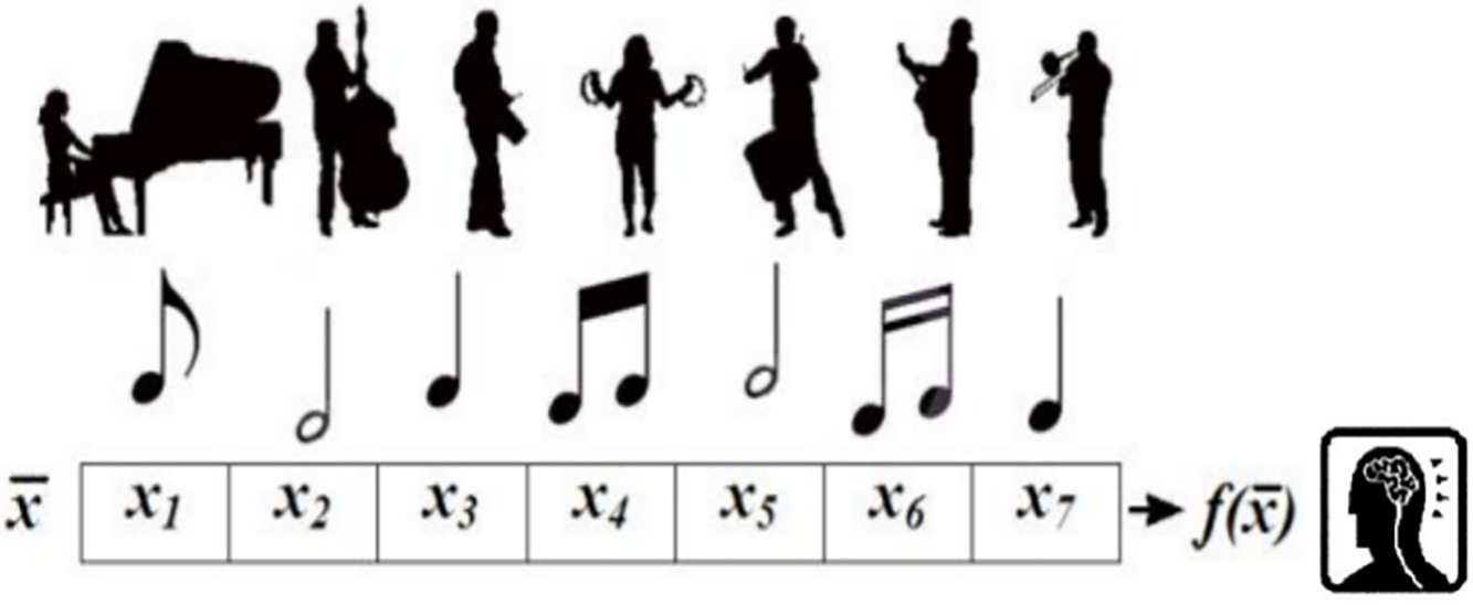
Figure 3: The mechanism of achieving harmonious and melodious music using the HS algorithm [41]

The HS algorithm has gained popularity due to its computational efficiency, simple implementation, limited parameters, and adaptability to both discrete and continuous optimization issues. It is widely applied in engineering, such as rock engineering structure design [43–45]. Compared to other meta-heuristic methods, the HS algorithm requires fewer mathematical demands, making it advantageous for diverse engineering problems.

The core steps of the HS algorithm to attain the best solution are outlined below:

Step 1: Define algorithm parameters and formulate the optimization problem. Key parameters include harmony memory size (HMS), harmony memory consideration rate (HMCR), pitch adjustment rate (PAR), bandwidth (bw), and the maximum number of repetitions (k).

Step 2: Randomly construct harmony memory by selecting values from the feasible range of decision variables.

Step 3: Generate a new harmony through three random selection mechanisms, incorporating harmony memory inspection and pitch adjustment rate. The new harmony vector adheres to allowable ranges. The selection rate from values stored in harmony memory is HMCR, and the remaining probability (1-HMCR) is assigned to random selection. For example, with HMCR set at 0.85, there is an 85% probability of selecting from ordered vectors and a 15% chance for random selection. If pitch adjustment is applied with probability PAR, it is modified by a random value within the specified bandwidth (see Fig. 4).

Step 4: Update the harmony memory by incorporating the new harmony vector. If the new harmony vector yields a better objective function value than the weakest harmony, it will replace the corresponding harmony in the memory. This update involves removing the harmony with the poorest objective function value, ensuring that the memory retains only the most optimal solutions.

Step 5: Repeat steps 3 and 4 until the stopping criterion (k) is met.

This process is illustrated in the flowchart shown in Fig. 5, which outlines the sequential steps of the HS algorithm [41].

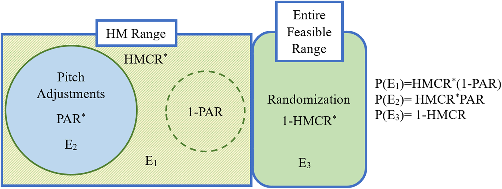
Figure 4: Verification of HMCR, PAR, and 1-HMCR [41]

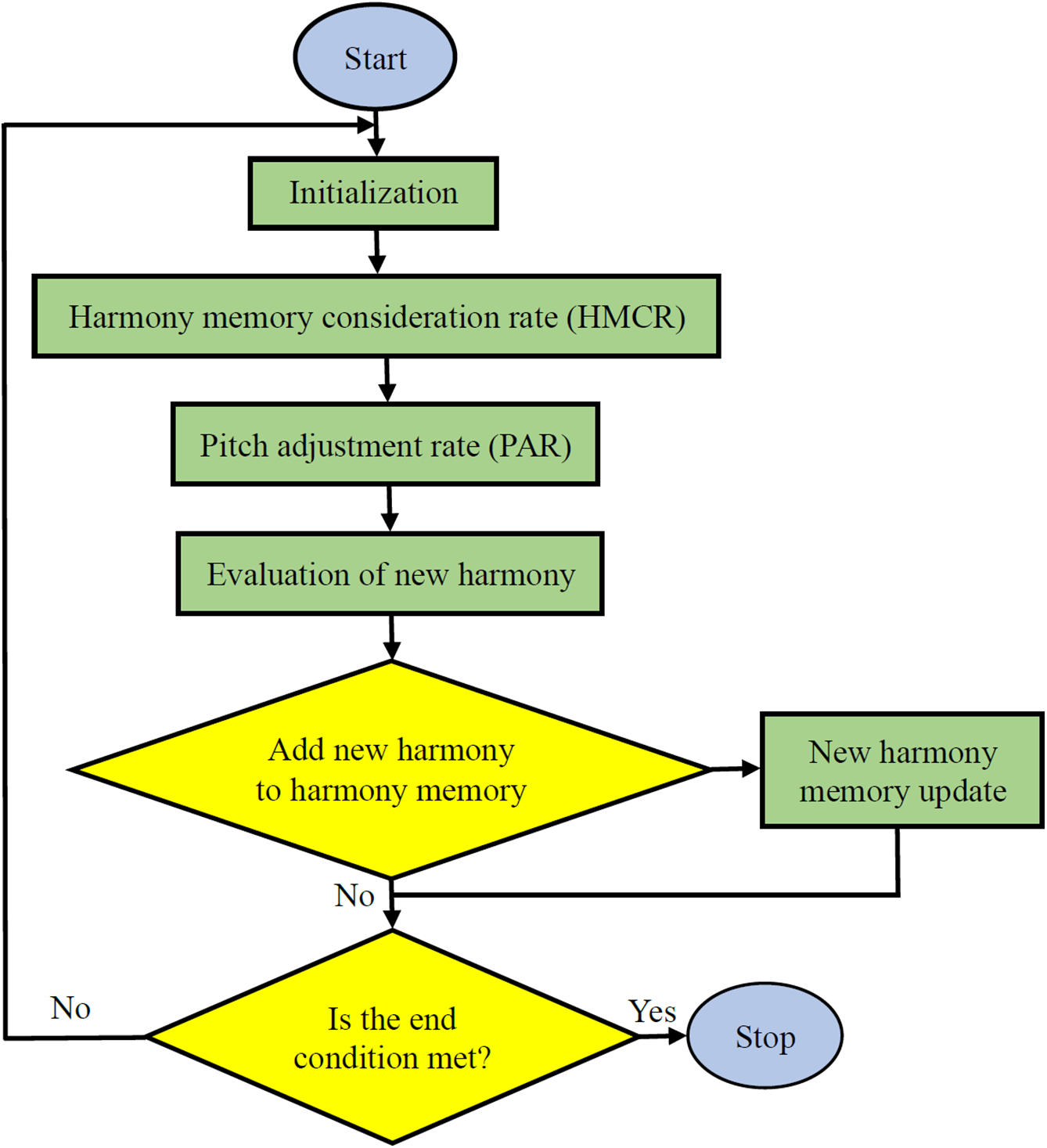
Figure 5: Flowchart illustrating the HS algorithm [41]

3.2 Teaching Learning-Based Optimization Algorithm (TLBO)

The TLBO algorithm, introduced by Rao et al. [46] for computer design problems, expanded to broader applications in 2012. Unlike other meta-heuristic methods that mimic natural processes, TLBO is inspired by classroom dynamics, simulating teacher-student interactions to find optimal solutions [47]. The algorithm’s iterative outcomes include students’ knowledge levels and performance scores. The subsequent sections elaborate on the various steps of this algorithm.

Initially, a set of points is generated and uniformly distributed across the problem-solving space, similar to students in a classroom. These points represent individual solutions. Values are calculated for all points, assuming a normal distribution of scores (Fig. 6) using the problem’s objective function. The top-performing student is designated as the teacher, initiating the training phase.

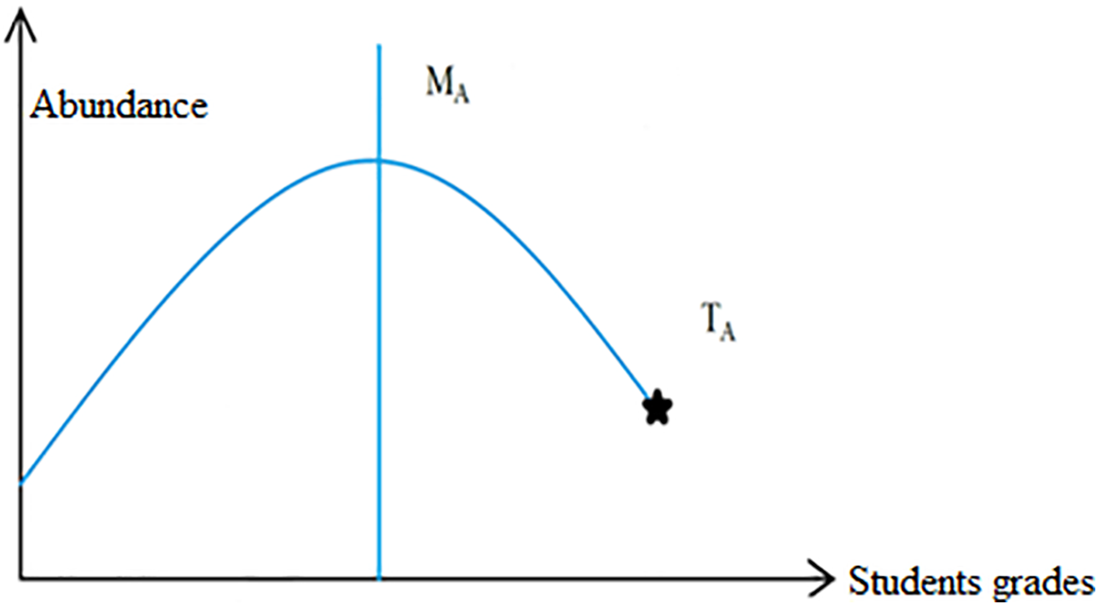
Figure 6: The initiation of population and teacher selection process [46]

The best-performing solution serves as the teacher, guiding other points towards its position, thus shifting the distribution mean towards the teacher. This shift includes a random element due to the randomized selection of points. The class average level (Mi) and the teacher’s level (Ti) determine the new average (Mnew), updating solutions based on the difference between current and new averages. This process is influenced by a random number (ri) and the teacher training factor (TF), which is either 1 or 2, chosen randomly (Fig. 7).

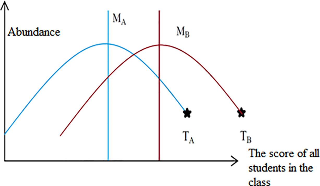
Figure 7: The transition of knowledge levels throughout the training phase [46]

3.3 Learning Phase

In this phase, students learn from each other. For each student, a second student is randomly chosen. If the second student’s objective function surpasses the first one, the first student adopts the second’s position, and vice versa. This process introduces variability and randomness. The algorithm then checks termination criteria; if not met, the loop restarts (Fig. 8).

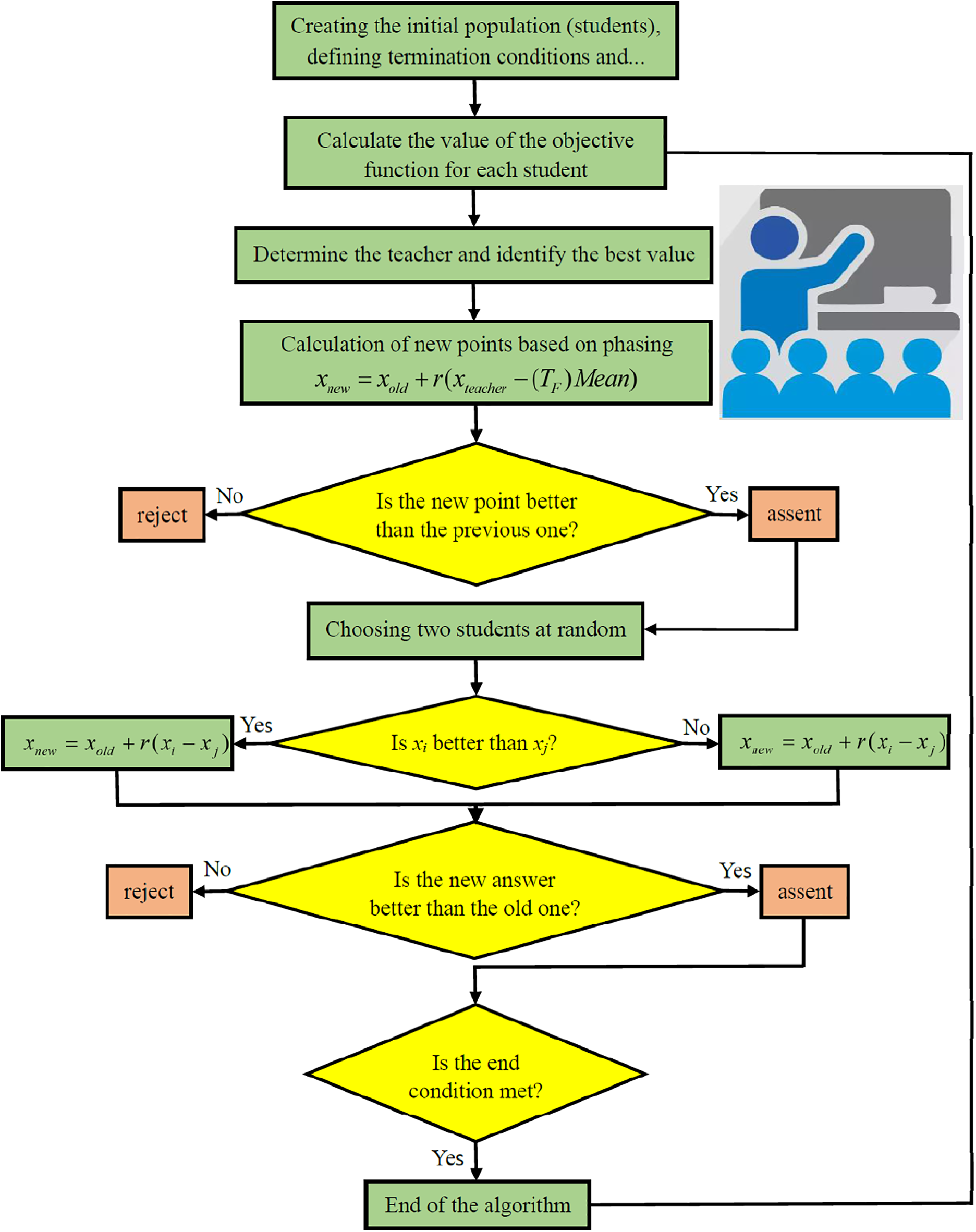
Figure 8: An overview of the TLBO algorithm through its flowchart [46]

The overarching objective of this study is to employ two robust and straightforward algorithms, namely HS and TLBO, for the prediction of Sm. Illustrating this endeavor, Fig. 9 depicts a schematic overview of the model’s architecture.

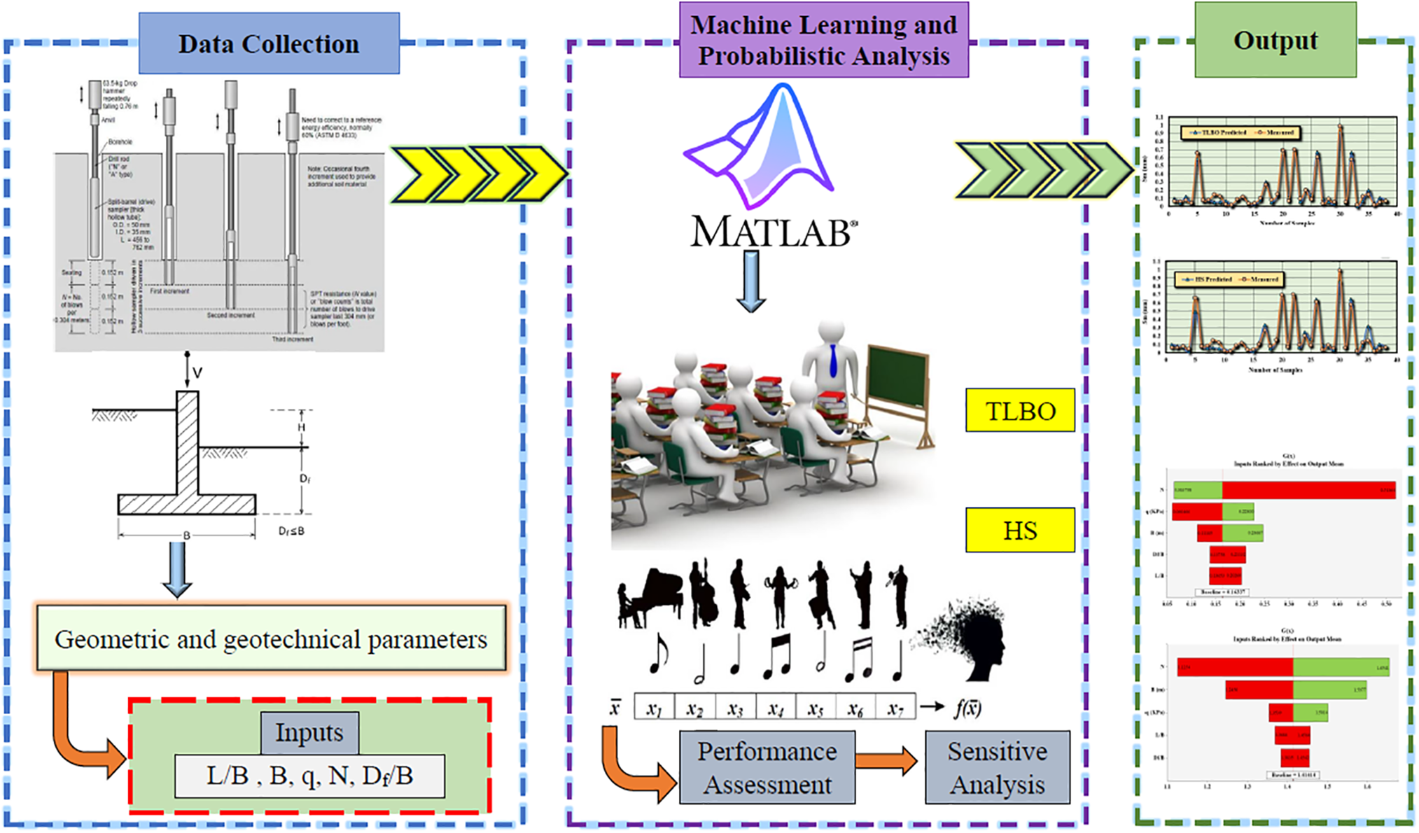
Figure 9: Architectural overview of the model (schematic representation)

4  Formulation and Sm Estimation via HS and TLBO Algorithms

The following sections of this study explore the prediction of Sm using the HS and TLBO algorithms. The integration of intelligent techniques provides a significant advantage with their simplicity and ability to handle geological uncertainties, nonlinearities, and complex relationships. This approach also accommodates a wide range of influential parameters that affect Sm, ensuring comprehensive coverage. In this methodology, the input and output data are systematically divided into training and testing sets. The training data are utilized to construct predictive models for Sm, while the test data are employed to evaluate and validate these models using statistical metrics. Out of 189 data points, 151 (representing 80% of the data) are allocated for training, while the remaining 38 data points (20% of the data) are reserved for model validation. In data-driven modeling, an initial data normalization step is typically performed to eliminate outliers and optimize results. Hence, Eq. (4) normalizes the values to a range between 0 and 1, where Xn denotes the normalized value, Xmea represents the actual value, Xmax is the maximum value, and Xmin indicates the minimum value.

Xn=[(Xmea−Xmin)/(Xmax−Xmin)](4)

After normalizing all 189 data points, the modeling process continued by using 80% of the data, equating to 151 data points, as training data. The HS and TLBO algorithms were utilized to build a nonlinear and complex predictive model. This was done by coding in the MATLAB environment. The model was developed through a trial-and-error approach, writing numerous relationships for the algorithms. This iterative process aimed to find the model with the lowest error, ensuring the algorithms were trained to their optimal performance. During this phase, various nonlinear and complex relationships were tested to identify the most accurate predictions. Among the relationships tested, Eq. (5) was found to be the most accurate, providing values closest to the actual data for predicting the Sm parameter. Therefore, Eq. (5) was chosen as the best equation from the trial-and-error process for both the HS and TLBO algorithms. This equation predicts Sm values with acceptable accuracy by incorporating five specific input parameters for this case study. The five input parameters were carefully selected based on their relevance and impact on the outcome, ensuring the model captured the underlying data complexities. The remaining 20% of the data was employed as test data to validate the robustness and accuracy of Eq. (5). This validation step was crucial to confirm the model’s reliability and predictive capability with new data points. The validation process of the constructed model involves comparing the predicted values from the test data with the actual observed values. If the test data, generated by the HS and TLBO algorithms for validation, closely aligns with the actual data (raw data) before modeling, it indicates that the model is highly accurate. Accordingly, various statistical measurement criteria can be applied. Based on the validation conducted and the successful application of Eq. (5), it can be concluded that the equation developed by the HS and TLBO algorithms is capable of effectively predicting complex scenarios. This approach highlighted the importance of iterative refinement and validation in model development, ensuring the final model was both accurate and generalizable to real-world applications. In addition, using MATLAB for coding and algorithm development facilitated efficient handling of complex computations and simulations. MATLAB’s robust environment and extensive libraries allowed for seamless integration of the HS and TLBO algorithms, enabling the researchers to focus on fine-tuning the model and interpreting the results. This study’s comprehensive approach, from initial data normalization to final validation, highlights the critical steps in developing a reliable predictive model. Each stage was meticulously executed to ensure the highest level of accuracy and reliability, demonstrating the potential of advanced algorithms such as HS and TLBO in predictive modeling.

Sm(mm)=−w1B(m)w2−w3q(KPa)w4−w5(10N)w6−w7L/Bw8−w9Df/Bw10−2w112(5)

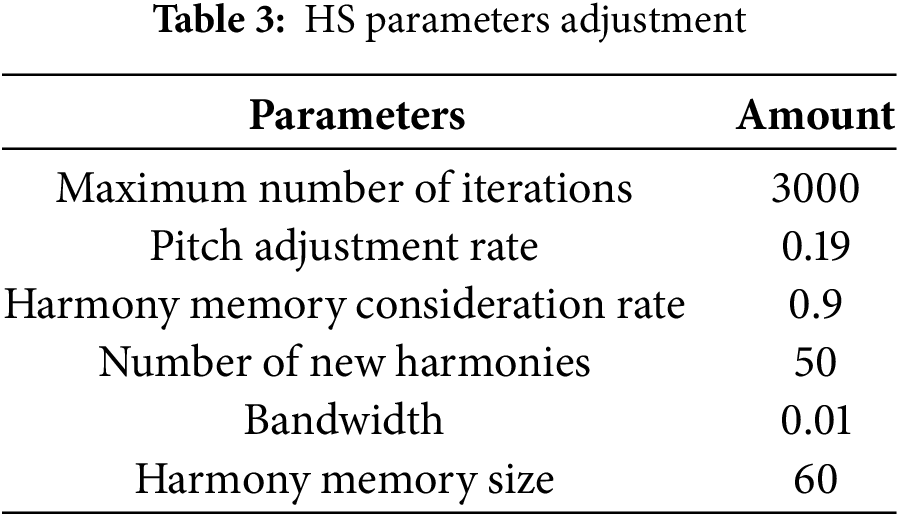
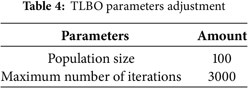
where wi is the weight factors corresponding to the input parameters. Achieving accurate Sm estimation with this equation relies on both the structure of the relationship and the adjustment parameters specific to the HS and TLBO algorithms. These parameters, which are determined through trial and error as well as user input, are essential for fine-tuning the models. The optimal models for HS and TLBO, utilizing the specified adjustment parameters, are detailed in Tables 3 and 4, respectively.

After formulating the equation and setting the parameters, the coefficients of the nonlinear predictive relations (wi) should be extracted to estimate Sm. For this purpose, Eq. (6) provides the coefficients of the model using the HS algorithm, and Eq. (7) provides the coefficients of the model using the TLBO algorithm.

Sm(mm)=0.1509B(m)0.2895+0.3673q(KPa)0.2846+0.38(10N)−0.6877−0.0216L/B0.5388−0.3279Df/B0.0012−2(0.1283)2(6)

Sm(mm)=0.6520B(m)0.4790+0.5647q(KPa)0.1044−0.3931(10N)0.3792−0.1422L/B6.0703+0.1424Df/B3.2091−2(−2.7651e−9)2(7)

5  Model Verification and Assessment

This study employs statistical metrics for validation to ensure the accuracy of the established relationship. Specifically, the R2, MSE, and RMSE are used as indicators to assess the prediction models for Sm using the HS and TLBO algorithms. These indicators are defined as follows:

R2=1−∑k=1n(tk−tk^)2∑k=1ntk2∑i=1nt2n(8)

MSE=1n∑k=1n(tk−tk^)2(9)

RMSE=1n∑k=1n(tk−tk^)2(10)

where n is the total number of samples, tk is the actual value, and tk^ is the predicted value for the kth observation. Smaller MSE and RMSE values closer to zero, along with R2 values closer to 1, signify a better-fitting model. When these conditions are met, the model demonstrates minimal error and closely aligns with the real-world context. Table 5 lists the evaluation outcomes for models constructed via the HS and TLBO algorithms.

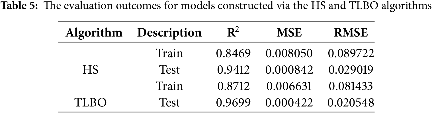
It is evident from the modeling outcomes that the relationships formulated using the HS and TLBO algorithms exhibit remarkable accuracy. For a more comprehensive understanding, the model outputs can be visually compared. Figs. 10 and 11 depict the comparison between actual and predicted values using the HS and TLBO algorithms for both training and testing datasets. The substantial overlap between the model outputs and actual values highlights the reliability and precision of the intelligent algorithms (HS and TLBO) in predicting and estimating Sm. In addition, these relationships can be extended to similar geological and tectonic scenarios (with comparable data) to effectively account for complexities and uncertainties in geotechnical parameters with a high degree of accuracy.

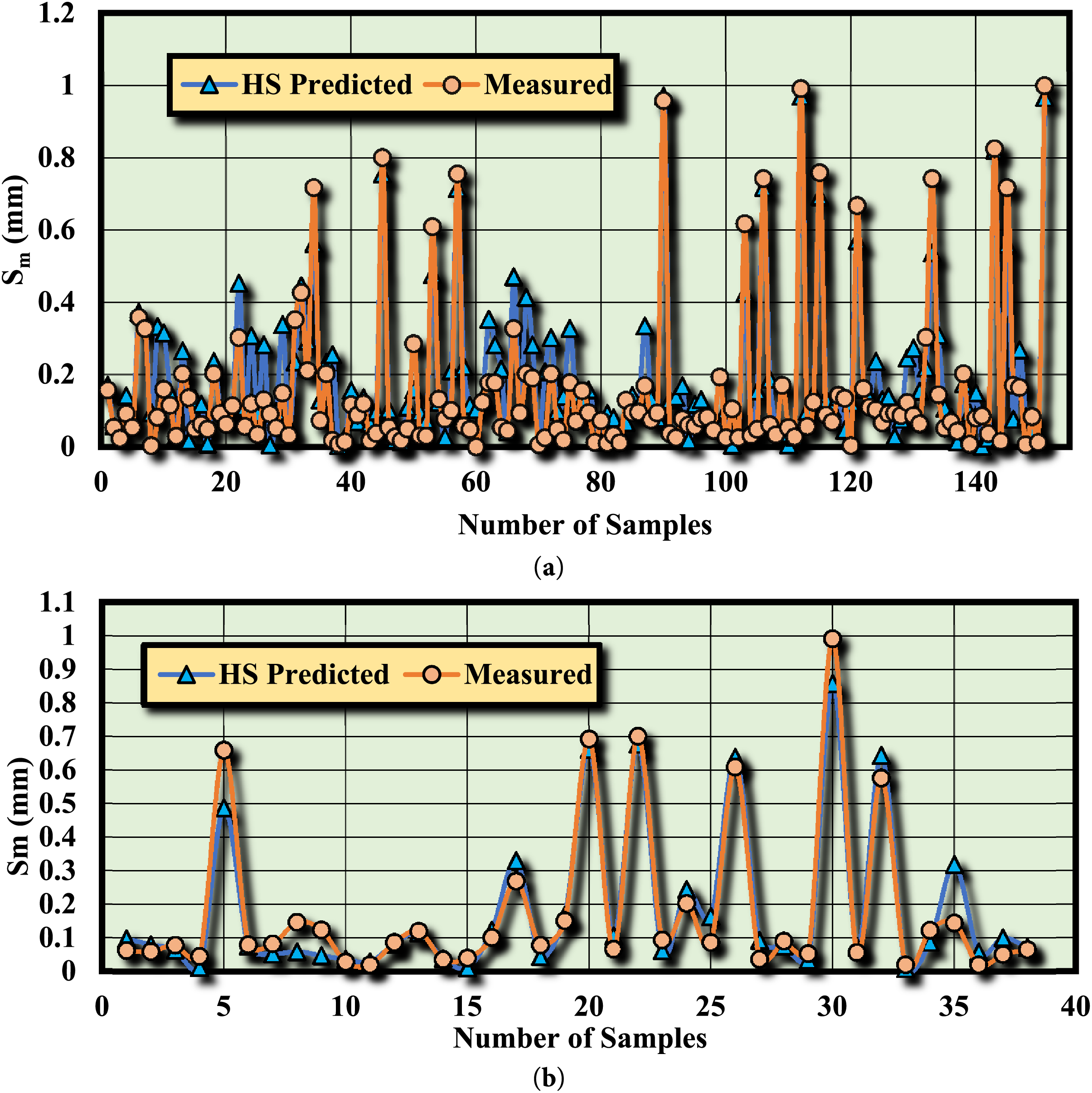
Figure 10: Comparison of Sm predictions by the HS algorithm and actual measurements for: (a) training data, (b) test data

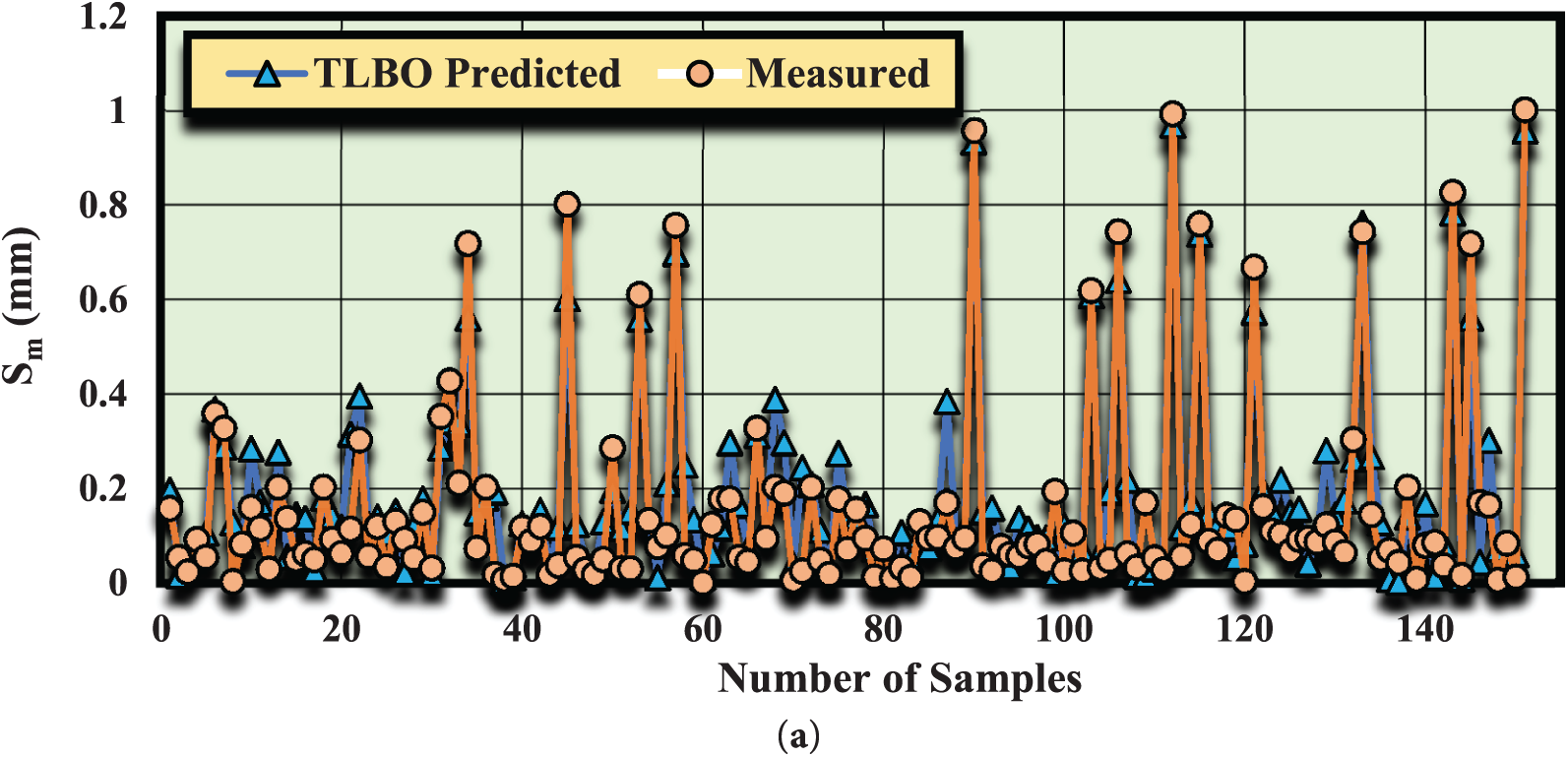
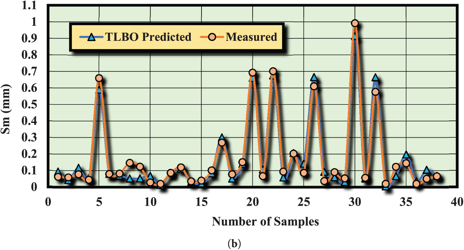
Figure 11: Comparison of Sm predictions by the TLBO algorithm and actual measurements for: (a) training data, (b) test data

6  Sensitivity Analysis

Given that the prediction model for Sm relies on five input parameters (N, q, B, Df/B, and L/B), it is crucial to understand the relative influence of these parameters on the model output. Sensitivity analysis allows us to determine which of these parameters has the greatest impact, helping to prioritize their importance. Using @RISK software, the correlation and ranking of these parameters can be analyzed within the model. The software employs a metric where the length of a parameter correlates with its effect on the model. In both models generated by the HS and TLBO algorithms, the parameter with the longest length has the greatest influence. Figs. 12 and 13 indicate that the parameter N appears with the longest length in both models, indicating its significant impact. Therefore, within the framework of the HS and TLBO algorithms, parameter N plays the most critical role in determining the model’s results. Even the smallest change in the N parameter leads to noticeable changes in the predicted Sm. N parameter is identified as highly sensitive, meaning minute fluctuations significantly affect the resulting predictions. Figs. 12 and 13 show that in both models, parameter N exhibits the longest length (Input High = 0.063, Input Low = 0.518), confirming its paramount importance. Therefore, parameter N’s sensitivity highlights its substantial impact on the Sm predictions.

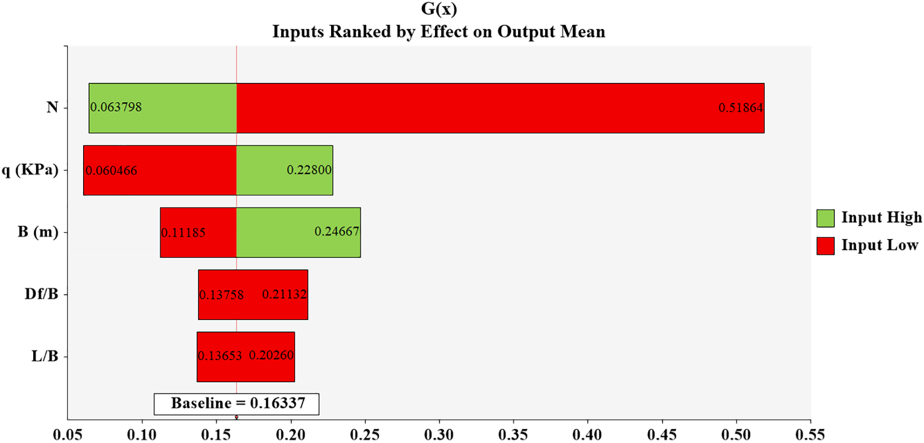
Figure 12: The results of the sensitivity analysis of the relationship created for the algorithm HS

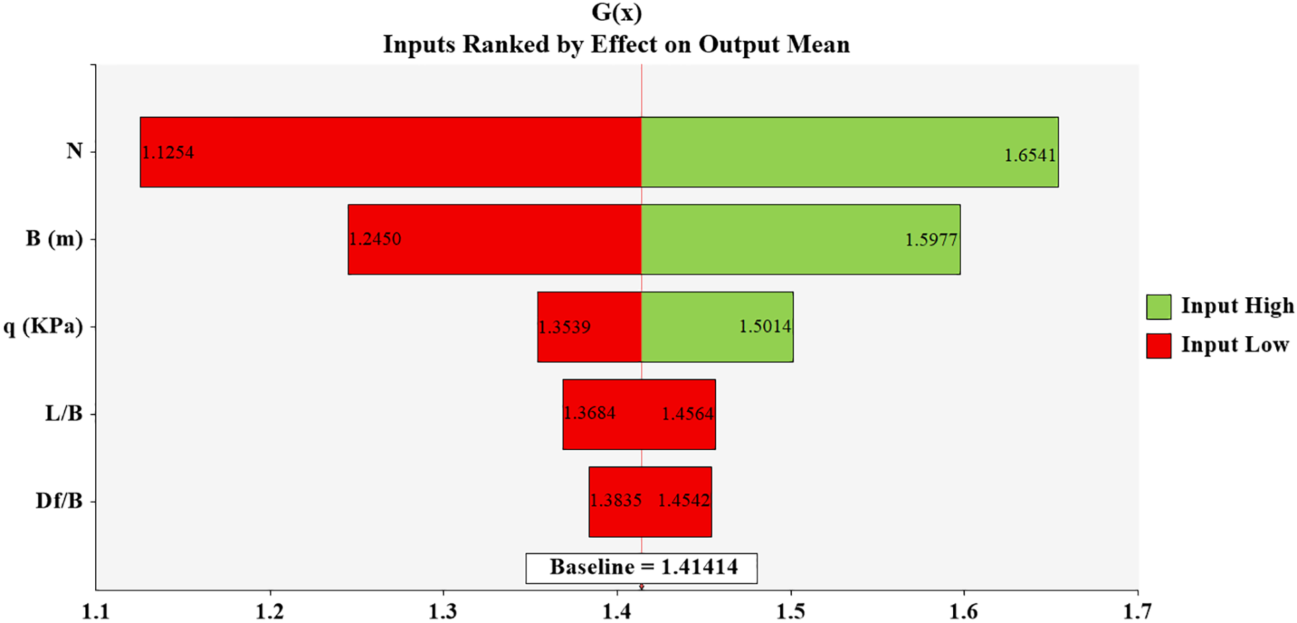
Figure 13: The results of the sensitivity analysis of the relationship created for the algorithm TLBO

7  Discussion

Considering the broad applicability and critical significance of Sm in geotechnical engineering and mining activities, directly determining this parameter involves considerable costs and time investment. In addition, errors induced by fatigue, stemming from frequent field and laboratory testing, can exacerbate concerns about accuracy. As an effective alternative, the use of indirect methods for calculating Sm provides a feasible solution. However, the inherent variability and uncertainty in the characteristics of soil and rock at different locations present challenges in achieving high precision with certain indirect methods, such as regression, experimental, analytical, and numerical approaches. In addition, these methods have the potential to comprehensively integrate all relevant influencing parameters (input variables) while remaining cost- and time-efficient.

This study concentrated on five key input parameters, B, q, N, Df/B, and L/B, which were identified as having the greatest impact on the model’s output. Sm estimation was performed using 189 data points through two optimization algorithms: HS and TLBO. In the model construction process, 80% of the data (151 data points) were randomly assigned for training, while the remaining 20% (38 data points) were used for model validation and evaluation. The validation process included statistical metrics such as the R2, MSE, and RMSE for both HS and TLBO algorithms applied to both the training and testing datasets. In addition, a sensitivity analysis of the parameters influencing the model’s output was conducted using @RISK software. The results revealed that the parameter N plays a dominant role in shaping the model’s output, indicating that even minor variations in N can lead to substantial fluctuations in Sm estimations. The findings clearly demonstrate the high accuracy achieved through the implementation of the HS and TLBO algorithms, mainly due to their close alignment with actual observed values.

The study successfully demonstrates the potential of TLBO and HS algorithms as powerful tools for addressing the complexities and uncertainties associated with Sm prediction. The developed models achieved exceptional accuracy, with R2 values exceeding 0.94 for both training and testing datasets, highlighting their reliability and robustness.

The practical implications for practitioners are significant. Engineers can achieve more accurate and cost-effective Sm predictions compared to traditional methods using TLBO and HS algorithms. Key applications include:

1.    Cost Reduction: The models enable Sm predictions using readily available parameters such as B, q, N, Df/B, and L/B, reducing the need for extensive site investigations and lowering overall project costs.

2.    Improved Design Accuracy: High prediction accuracy ensures that foundation designs are based on reliable data, minimizing risks of overdesign or underdesign and enhancing structural safety.

3.    Integration into Existing Workflows: The simplicity and adaptability of the algorithms make them easy to incorporate into existing geotechnical workflows, requiring minimal additional training and computational resources.

4.    Handling Uncertainty: The robustness of TLBO and HS in managing nonlinear relationships and uncertainties makes them ideal for complex geotechnical scenarios where traditional methods can be insufficient.

5.    Scalability across Projects: The models’ adaptability allows them to be applied across various project scales, from small residential foundations to significant infrastructure developments, with minor adjustments to suit specific geological conditions.

Although this study primarily focused on soil and foundation parameters for settlement prediction under static conditions, future research can explore the inclusion of dynamic load scenarios, such as near and far field motions, to further refine the model’s predictive capabilities. In addition, incorporating Soil-Structure Interaction (SSI) effects will enhance the model’s ability to capture complex interaction phenomena, leading to more accurate and reliable predictions across diverse conditions. Practitioners are encouraged to validate the models against local site-specific data to ensure their suitability for regional applications.

8  Conclusion

This study highlights the effectiveness of TLBO and HS algorithms in predicting Sm with high accuracy. The models developed achieved R2 values exceeding 0.94, demonstrating their reliability and robustness. The findings provide valuable insights for geotechnical engineers, enabling more accurate, cost-effective, and efficient settlement predictions. Practitioners can enhance design accuracy, reduce project costs, and improve overall geotechnical analysis by implementing these algorithms. The results highlight the potential of machine learning approaches in addressing the challenges associated with geotechnical parameter estimation, contributing to safer and more sustainable construction practices.

Acknowledgement: Not applicable.

Funding Statement: The authors received no specific funding for this study.

Author Contributions: Study conception and design: Hadi Fattahi; data collection: Hadi Fattahi; analysis and interpretation of results: Danial Jahed Armaghani, Hossein Ghaedi; supervision: Hadi Fattahi; draft manuscript preparation: Danial Jahed Armaghani, Hadi Fattahi. All authors reviewed the results and approved the final version of the manuscript.

Availability of Data and Materials: All data and models used or generated during the study are included in the published article. The corresponding author can provide the study’s code upon request.

Ethics Approval: Not applicable.

Conflicts of Interest: The authors declare no conflicts of interest to report regarding the present study.

References

1. Boushehrian AH, Hataf N, Ghahramani A. Modeling of the cyclic behavior of shallow foundations resting on geomesh and grid-anchor reinforced sand. Geotext Geomembr. 2011;29(3):242–8. doi:10.1016/j.geotexmem.2010.11.008. [Google Scholar] [CrossRef]

2. Moghaddas Tafreshi SN, Dawson AR. Behaviour of footings on reinforced sand subjected to repeated loading-Comparing use of 3D and planar geotextile. Geotext Geomembr. 2010;28(5):434–47. doi:10.1016/j.geotexmem.2009.12.007. [Google Scholar] [CrossRef]

3. Fattah MY, Karim HH, Al-Qazzaz HH. Effect of embedment depth on cyclic behavior of tank footings on dry sand. Transp Infrastruct Geotechnol. 2022;9(2):220–35. doi:10.1007/s40515-021-00164-9. [Google Scholar] [CrossRef]

4. Li T, Baus RL. Nonlinear parameters for granular base materials from plate tests. J Geotech Geoenviron Eng. 2005;131(7):907–13. doi:10.1061/(ASCE)1090-0241(2005)131:7(907). [Google Scholar] [CrossRef]

5. Jagan J, Samui P. AI-powered simulation models for estimating the consolidation settlement of shallow foundations. Model Earth Syst Environ. 2024;11(1):1. doi:10.1007/s40808-024-02221-x. [Google Scholar] [CrossRef]

6. Li J, Wu J, Hu W. A hybrid learning approach for simulating settlement of shallow foundation. Multiscale Multidiscip Model Exp Des. 2024;8(1):9. doi:10.1007/s41939-024-00638-6. [Google Scholar] [CrossRef]

7. Fioravante V, Giretti D, Masella A, Vaciago G. Settlement prediction of shallow foundations for quality controls of sandy hydraulic fills. Soils Found. 2024;64(1):101408. doi:10.1016/j.sandf.2023.101408. [Google Scholar] [CrossRef]

8. Kusakabe O. Experiment and analysis on the scale effect of Nγ for circular and rectangular footings. In: Centrifuge 91: Proceedings of the International Conference Centrifuge 1991; 1991 Jun 13–14; Boulder, CO, USA. p. 179–89. [Google Scholar]

9. Khing KH, Das BM, Puri VK, Cook EE, Yen SC. The bearing-capacity of a strip foundation on geogrid-reinforced sand. Geotext Geomembr. 1993;12(4):351–61. doi:10.1016/0266-1144(93)90009-D. [Google Scholar] [CrossRef]

10. Shahir H, Pak A. Estimating liquefaction-induced settlement of shallow foundations by numerical approach. Comput Geotech. 2010;37(3):267–79. doi:10.1016/j.compgeo.2009.10.001. [Google Scholar] [CrossRef]

11. Foye KC, Basu P, Prezzi M. Immediate settlement of shallow foundations bearing on clay. Int J Geomech. 2008;8(5):300–10. doi:10.1061/(ASCE)1532-3641(2008)8:5(300). [Google Scholar] [CrossRef]

12. Eid HT. Bearing capacity and settlement of skirted shallow foundations on sand. Int J Geomech. 2013;13(5):645–52. doi:10.1061/(ASCE)GM.1943-5622.0000237. [Google Scholar] [CrossRef]

13. Kim Y, Park H, Jeong S. Settlement behavior of shallow foundations in unsaturated soils under rainfall. Sustainability. 2017;9(8):1417. doi:10.3390/su9081417. [Google Scholar] [CrossRef]

14. Cong S, Tang L, Ling X, Geng L, Lu J. Numerical analysis of liquefaction-induced differential settlement of shallow foundations on an island slope. Soil Dyn Earthq Eng. 2021;140(6):106453. doi:10.1016/j.soildyn.2020.106453. [Google Scholar] [CrossRef]

15. Hakro MR, Kumar A, Ali M, Habib AF, de Azevedo ARG, Fediuk R, et al. Numerical analysis of shallow foundations with varying loading and soil conditions. Buildings. 2022;12(5):693. doi:10.3390/buildings12050693. [Google Scholar] [CrossRef]

16. Tabaroei A, Abrishami S, Seyedi Hosseininia E, Ganjian N. A study on bearing capacity of circular footing resting on geogrid reinforced granular soil. Amirkabir J Civ Eng. 2018;50(5):973–86. doi:10.22060/ceej.2017.13150.5339. [Google Scholar] [CrossRef]

17. Tasiopoulou P, Chaloulos Y, Gerolymos N, Giannakou A, Chacko J. 3D and 2D simulations of liquefaction induced settlements of shallow foundations using Ta-Ger model. In: Earthquake geotechnical engineering for protection and development of environment and constructions. Boca Raton, FL, USA: CRC Press; 2019. p. 5241–8. [Google Scholar]

18. Zhu F, Clark JI, Phillips R. Scale effect of strip and circular footings resting on dense sand. J Geotech Geoenviron Eng. 2001;127(7):613–21. doi:10.1061/(ASCE)1090-0241(2001)127:7(613). [Google Scholar] [CrossRef]

19. McMahon BT, Haigh SK, Bolton MD. Bearing capacity and settlement of circular shallow foundations using a nonlinear constitutive relationship. Can Geotech J. 2014;51(9):995–1003. doi:10.1139/cgj-2013-0275. [Google Scholar] [CrossRef]

20. Momeni E, He B, Abdi Y, Jahed Armaghani D. Novel hybrid XGBoost model to forecast soil shear strength based on some soil index tests. Comput Model Eng Sci. 2023;136(3):2527–50. doi:10.32604/cmes.2023.026531. [Google Scholar] [CrossRef]

21. Shahin MA, Maier HR, Jaksa MB. Predicting settlement of shallow foundations using neural networks. J Geotech Geoenviron Eng. 2002;128(9):785–93. doi:10.1061/(ASCE)1090-0241(2002)128:9(785). [Google Scholar] [CrossRef]

22. Samui P. Support vector machine applied to settlement of shallow foundations on cohesionless soils. Comput Geotech. 2008;35(3):419–27. doi:10.1016/j.compgeo.2007.06.014. [Google Scholar] [CrossRef]

23. Soleimanbeigi A, Hataf N. Prediction of settlement of shallow foundations on reinforced soils using neural networks. Geosynth Int. 2006;13(4):161–70. doi:10.1680/gein.2006.13.4.161. [Google Scholar] [CrossRef]

24. Shahin MA, Jaksa MB, Maier HR. Predicting the settlement of shallow foundations on cohesionless soils using back-propagation neural networks. Adelaide, SA, Australia: Department of Civil and Environmental Engineering, University of Adelaide; 2000. [Google Scholar]

25. Gnananandarao T, Dutta R, Khatri V. Application of artificial neural network to predict the settlement of shallow foundations on cohesionless soils. In: Geotechnical applications. Berlin/Heidelberg, Germany: Springer; 2019. p. 51–8. [Google Scholar]

26. Luat N-V, Nguyen V-Q, Lee S, Woo S, Lee K. An evolutionary hybrid optimization of MARS model in predicting settlement of shallow foundations on sandy soils. Geomech Eng. 2020;21(6):583–98. doi:10.12989/gae.2020.21.6.583. [Google Scholar] [CrossRef]

27. Shahin MA, Maier HR, Jaksa MB. Settlement prediction of shallow foundations on granular soils using B-spline neurofuzzy models. Comput Geotech. 2003;30(8):637–47. doi:10.1016/j.compgeo.2003.09.004. [Google Scholar] [CrossRef]

28. Mohammed M, Sharafati A, Al-Ansari N, Yaseen ZM. Shallow foundation settlement quantification: application of hybridized adaptive neuro-fuzzy inference system model. Adv Civ Eng. 2020;2020(1):7381617. doi:10.1155/2020/7381617. [Google Scholar] [CrossRef]

29. Shahin M, Jaksa M, Maier H. Stochastic simulation of settlement prediction of shallow foundations based on a deterministic artificial neural network model. Rome, Italy: Food and Agriculture Organization of the United Nations; 2005. [Google Scholar]

30. Wan X. Predicting the settlement of shallow foundation using metaheuristic SVR approaches. Geotech Geol Eng. 2023;41(8):4795–805. doi:10.1007/s10706-023-02547-w. [Google Scholar] [CrossRef]

31. Krishna Pradeep P, Sankar N, Chandrakaran S. Settlement prediction of shallow foundations on cohesionless soil using hybrid PSO-ANN approach. In: Proceedings of SECON’21: Structural Engineering and Construction Management; 2021 May 12–15; Online. p. 1005–14. [Google Scholar]

32. Tsai H-C, Tyan Y-Y, Wu Y-W, Lin Y-H. Determining ultimate bearing capacity of shallow foundations using a genetic programming system. Neural Comput Appl. 2013;23(7-8):2073–84. doi:10.1007/s00521-012-1150-8. [Google Scholar] [CrossRef]

33. Ray R, Kumar D, Samui P, Roy LB, Goh ATC, Zhang W. Application of soft computing techniques for shallow foundation reliability in geotechnical engineering. Geosci Front. 2021;12(1):375–83. doi:10.1016/j.gsf.2020.05.003. [Google Scholar] [CrossRef]

34. Akca N. Correlation of SPT-CPT data from the united Arab emirates. Eng Geol. 2003;67(3–4):219–31. doi:10.1016/S0013-7952(02)00181-3. [Google Scholar] [CrossRef]

35. Hettiarachchi H, Brown T. Use of SPT blow counts to estimate shear strength properties of soils: energy balance approach. J Geotech Geoenvironmental Eng. 2009;135(6):830–4. doi:10.1061/(ASCE)GT.1943-5606.0000016. [Google Scholar] [CrossRef]

36. Akin MK, Kramer SL, Topal T. Empirical correlations of shear wave velocity (Vs) and penetration resistance (SPT-N) for different soils in an earthquake-prone area (Erbaa-Turkey). Eng Geol. 2011;119(1):1–17. doi:10.1016/j.enggeo.2011.01.007. [Google Scholar] [CrossRef]

37. Nassaji F, Kalantari B. SPT capability to estimate undrained shear strength of fine-grained soils of Tehran. Iran Electron J Geotech Eng. 2011;16(2011):1229–38. [Google Scholar]

38. Burland J, Burbidge M, Wilson E, Terzaghi. Settlement of foundations on sand and gravel. Proc Inst Civ Eng. 1985;78(6):1325–81. doi:10.1680/iicep.1985.1058. [Google Scholar] [CrossRef]

39. Terzaghi K, Peck RB. Soil mechanics. In: Engineering practice. New York, NY, USA: John Wiley & Sons, Inc. 1948. [Google Scholar]

40. Zhang W, Li H, Wu C, Li Y, Liu Z, Liu H. Soft computing approach for prediction of surface settlement induced by earth pressure balance shield tunneling. Undergr Space. 2021;6(4):353–63. doi:10.1016/j.undsp.2019.12.003. [Google Scholar] [CrossRef]

41. Geem ZW, Kim JH, Loganathan GV. A new heuristic optimization algorithm: harmony search. Simulation. 2001;76(2):60–8. doi:10.1177/003754970107600201. [Google Scholar] [CrossRef]

42. Fattahi H, Gholami A, Amiribakhtiar MS, Moradi S. Estimation of asphaltene precipitation from titration data: a hybrid support vector regression with harmony search. Neural Comput Appl. 2015;26(4):789–98. doi:10.1007/s00521-014-1766-y. [Google Scholar] [CrossRef]

43. Manahiloh KN, Nejad MM, Momeni MS. Optimization of design parameters and cost of geosynthetic-reinforced earth walls using harmony search algorithm. Int J Geosynth Ground Eng. 2015;1(4):1–12. doi:10.1007/s40891-015-0039-x. [Google Scholar] [CrossRef]

44. Mikaeil R, Shaffiee Haghshenas S, Shirvand Y, Valizadeh Hasanluy M, Roshanaei V. Risk assessment of geological hazards in a tunneling project using harmony search algorithm (case study: Ardabil-mianeh railway tunnel). Civ Eng J. 2016;2(10):546–54. doi:10.28991/cej-2016-00000057. [Google Scholar] [CrossRef]

45. Afradi A, Ebrahimabadi A, Hallajian T. Prediction of TBM penetration rate using fuzzy logic, particle swarm optimization and harmony search algorithm. Geotech Geol Eng. 2022;40(3):1513–36. doi:10.1007/s10706-021-01982-x. [Google Scholar] [CrossRef]

46. Rao RV, Savsani VJ, Vakharia D. Teaching-learning-based optimization: an optimization method for continuous non-linear large scale problems. Inf Sci. 2012;183(1):1–15. doi:10.1016/j.ins.2011.08.006. [Google Scholar] [CrossRef]

47. Fattahi H, Ghaedi H, Malekmahmoodi F. Prediction of rock drillability using gray wolf optimization and teaching-learning-based optimization techniques. Soft Comput. 2024;28(1):461–76. doi:10.1007/s00500-023-08233-6. [Google Scholar] [CrossRef]